Simple and Nearly Optimal Polynomial Root-finding by Means of Root Radii Approximation

Abstract

We propose a new simple but nearly optimal algorithm for the approximation of all sufficiently well isolated complex roots and root clusters of a univariate polynomial. Quite typically the known root-finders at first compute some crude but reasonably good approximations to well-conditioned roots (that is, those isolated from the other roots) and then refine the approximations very fast, by using Boolean time which is nearly optimal, up to a polylogarithmic factor. By combining and extending some old root-finding techniques, the geometry of the complex plane, and randomized parametrization, we accelerate the initial stage of obtaining crude to all well-conditioned simple and multiple roots as well as isolated root clusters. Our algorithm performs this stage at a Boolean cost dominated by the nearly optimal cost of subsequent refinement of these approximations, which we can perform concurrently, with minimum processor communication and synchronization. Our techniques are quite simple and elementary; their power and application range may increase in their combination with the known efficient root-finding methods.

Keywords:

Polynomials; Root-finding; Root isolation; Root radii

1 Introduction

1.1 The problem and our progress

We seek the roots $x_{1},\dots,x_{n}$ of a univariate polynomial of degree $n$ with real or complex coefficients,

$$p(x)=\sum^{n}_{i=0}p_{i}x^{i}=p_{n}\prod^{n}_{j=1}(x-x_{j}),~{}~{}~{}p_{n}\neq 0.$$ (1)

This classical problem is four millennia old, but is still important, e.g., for Geometric Modeling, Control, Robotics, Global Optimization, Financial Mathematics, and Signal and Image Processing (cf. [MP13, Preface]).

Quite typically a fast root-finder consists of two stages. At first one computes some crude but reasonably good approximations to well-conditioned roots (that is, those isolated from the other roots) and then refines the approximations very fast, within nearly optimal Boolean time. Here and hereafter “nearly optimal” means “optimal up to a polylogarithmic factor”, and we measure the isolation of two roots $x_{g}$ and $x_{h}$ from one another by the ratio $|x_{g}-x_{h}|/\max_{1\leq i,j\leq n}|x_{g}-x_{j}|$.

We obtain substantial progress at the initial stage of computing crude but reasonably close initial approximations to all well-conditioned and possibly multiple roots. The Boolean cost of performing our algorithm can be complemented by the nearly optimal Boolean cost of refining our initial approximation by means of the algorithms of [PT13], [PT14], [PT15], and [PT16]. By combining them with our present algorithm, we approximate all well-conditioned roots of a polynomial by matching the record and nearly optimal Boolean complexity bound of [P95] and [P02]. Our present algorithm, however, is much less involved, more transparent and more accessible for the implementation (see the next subsection).

Approximation of the well-conditioned roots is already an important sub-problem of the root-finding problem, but can also facilitate the subsequent approximation of the ill-conditioned roots. E.g., having approximated the well-conditioned roots $1$, $-1$, $\sqrt{-1}$, and $-\sqrt{-1}$ of the polynomial $p(x)=(x^{4}-1)(x^{4}-10^{-200})$, we can deflate it explicitly or implicitly (cf. [PT16]) and more readily approximate its ill-conditioned roots $10^{-50}$, $-10^{-50}$, $10^{-50}\sqrt{-1}$, and $-10^{-50}\sqrt{-1}$ as the well-conditioned roots of the deflated polynomial $x^{4}-10^{-200}$ (cf. the first paragraph of Sect. 5).

Moreover, our algorithm can be readily extended to computing crude approximations of small discs covering all isolated root clusters. Then again the Boolean cost of this computation is dominated by the cost of the refinement of the computed approximations to the clusters.

Clearly, the refinement of well-conditioned roots and root clusters can be performed concurrently, with minimum communication and synchronization among the processors. The existence of non-isolated roots and root clusters little affects our algorithm; our cost estimate does not depend on the minimal distance between the roots and includes no terms like $\log({\rm Discr}(p)^{-1})$.

1.2 Our technical means

We achieve our progress by means of exploiting the geometry of the complex plane, randomized parametrization, and an old algorithm of [S82], which approximates all root radii of a polynomial, that is, the distances from all roots to the origin, at a low Boolean cost. We refer the reader to [O40], [G72], [H74], and [B79] on the preceding works related to that algorithm and cited in [S82, Section 14] and [P00, Section 4], and one can also compare the relevant techniques of the power geometry in [B79] and [B98], developed for the study of algebraic and differential equations. By combining the root-radii algorithm with a shift of the origin, one readily extends it to fast approximation of the distances of all roots to any selected point of the complex plane (see Corollary 1).

Computations of our algorithm amount essentially to approximation of the root radii of three polynomials obtained from a polynomial $p(x)$ by means of three shifts of the variable $x$, versus many more computations of this kind and application of many other nontrivial techniques in the algorithm of [P95] and [P02]. This makes it much harder to implement and even to comprehend than our present algorithm.

Schönhage in [S82] used only a small part of the potential power of his root-radii algorithm by applying it to the rather modest auxiliary task of the isolation of a single complex root, and we restricted ourselves to similar auxiliary applications in [P95] and [P02]. The algorithm and its basic concept of Newton’s polygon, however, deserves greater attention of the researchers in polynomial root-finding.

In the next two subsections we outline our algorithms of [PZ15] and the present paper [PZ15], which should demonstrate the power of our approach.

1.3 Approximation of Well-Conditioned Real Roots: An Outline

It is instructive to recall the algorithm of [PZ15], which approximates all simple and well-conditioned real roots in nearly optimal Boolean time. At first it approximates all the $n$ root radii. They define $n$ narrow annuli at the complex plane, all of them centered at the origin and each of them containing a root of the polynomial $p(x)$. Multiple roots define multiple annuli. Clusters of roots define clusters of overlapping annuli. The intersections of at most n narrow annuli with the real axis define at most $2n$ small intervals,which contain all real roots. By applying to these intervals a known efficient real root-refiner, e.g., that of [PT16], [PT16], we readily approximate all well-conditioned at a nearly optimal Boolean cost.

In [PZ15] the resulting real root-finder was tested for some benchmark polynomials, each having a small number of real roots. The tests, performed numerically, with the IEEE standard double precision, gave encouraging results; in particular the number of the auxiliary root-squaring iterations (3) grew very slowly as the degree of input polynomials increased from 64 to 1024.

1.4 Approximation of Well-Conditioned Complex Roots: An Outline

Next we outline our main algorithm, which we specify in some detail and analyze in Sect. 4.1. The algorithm approximates the well-conditioned complex roots of a polynomial by means of incorporating the root-radii algorithm into a rather sophisticated construction on the complex plane.

At first we compute a sufficiently large positive value $r^{+}_{1}$ such that the disc $D=\{x:~{}|x|\leq r^{+}_{1}\}$ on the complex plane contains all roots of $p(x)$. Then we approximate the distances to the roots from the two points, $\eta r^{+}_{1}$ on the real axis and $\eta r^{+}_{1}\sqrt{-1}$ on the imaginary axis, for a reasonably large value of $\eta$, so that these two points lie reasonably far from the disc $D$.

Having the distances approximated, we obtain two families of narrow annuli centered at the latter pair of points. Each family is made up of $n$ annuli that contain the $n$ roots of a polynomial $p(x)$, all lying in the disc $D$. Its intersections with the annuli are closely approximated by $n$ narrow vertical and $n$ narrow horizontal rectangles on the complex plane. Every root lies in the intersection of two rectangles of the vertical and horizontal families, and there are $N\leq n^{2}$ intersections overall, each approximated by a square.

At most $n_{-}$ squares contain all $n_{-}\leq n$ well-conditioned roots of a polynomial $p(x)$, and we can identify these squares by evaluating $p(x)$ or applying proximity tests at the centers of $N$ candidate squares (and then we would discard the other $N-n_{-}$ squares). The cost of these computations would be prohibitively large, however, and so instead we identify the desired $n_{-}$ squares probabilistically, by applying the root-radii algorithm once again.

This time we approximate the distances to all the $n$ roots from a complex point $\eta r^{+}_{1}\exp(\frac{\gamma~{}\sqrt{-1}}{2\pi})$ where we choose the angle $\gamma$ at random in a fixed range. Having the distances approximated, we obtain at most $n_{-}$ narrow rectangles that contain all the $n$ roots. The long sides of the rectangles are directed at the angle $\gamma$ to the real axis. We choose the range for $\gamma$ such that with a probability close to 1 each rectangle intersects a single square. Then we readily compute the centers of all these squares in a nearly optimal randomized Boolean time and notice that all the well-conditioned roots are expected to be closely approximated by some of these centers. We can refine these approximations readily by applying the efficient algorithms of [K98] or [PT16].

1.5 Organization of our paper

We organize our presentation as follows. In the next two sections we recall some auxiliary results. In Section 4 we describe our main algorithm. In Section 5 we briefly comment on some directions to its strengthening and extension.

2 Some Definitions and Auxiliary Results

Hereafter “flop” stands for “arithmetic operation”, and “$\lg$” stands for “$\log_{2}$”.

$O_{B}(\cdot)$ and $\tilde{O}_{B}(\cdot)$ denote the Boolean complexity up to some constant and poly-logarithmic factors, respectively.

$||p(x)||=\max_{i=0}^{n}|p_{i}|$; $\tau=\lg(||p(x)||+\frac{1}{||p(x)||})$ for a polynomial $p(x)$ of (1).

Definition 1

$D(z,\rho)=\{x:~{}|x-z|\leq\rho\}$ denotes the closed disc with a complex center $z$ and a radius $\rho$. Such a disc is $\gamma$-isolated, for $\gamma>1$, if the disc $D(z,\gamma\rho)$ contains no other roots of a polynomial $p(x)$ of equation (1). Its root $x_{j}$ is $\gamma$-isolated if no other roots of the polynomial $p(x)$ lie in the disc $D(x_{j},(\gamma+1)|x_{j}|)$.

Suppose that some crude but reasonably close approximations to the set of well-isolated roots of a polynomial are available. Then, by applying the algorithms of [K98] or [PT14], [PT16], one can refine these approximations to the roots at a low Boolean cost. In the rest of our paper we present and analyze our new algorithm for computing such crude initial approximations to the well-isolated roots.

3 Approximation of Root Radii and Distances to Roots

Definition 2

List the absolute values of the roots of $p(x)$ in non-increasing order, denote them $r_{j}=|x_{j}|$ for $j=1,\dots,n$, $r_{1}\geq r_{2}\geq\cdots\geq r_{n}$, and call them the root radii of the polynomial $p(x)$.

The following theorem bounds the largest root radius $r_{1}$, and then we bound the Boolean cost of the approximation of all root radii.

Theorem 3.1

(See [VdS70].) For a polynomial $p(x)$ of (1) and $r_{1}=\max_{j=1}^{n}|x_{j}|$, it holds that

$$0.5r_{1}^{+}/n\leq r_{1}\leq r_{1}^{+}~{}{\rm for}~{}r_{1}^{+}=2\max_{i=1}^{n}|p_{n-i}/p_{n}|.$$ (2)

Theorem 3.2

Assume that we are given a polynomial $p=p(x)$ of (1) and $\theta>1$. Then, within the Boolean cost bound $\tilde{O}_{B}(\tau n+n^{2})$, one can compute approximations $\tilde{r}_{j}$ to all root radii $r_{j}$ such that $1/\theta\leq\tilde{r}_{j}/r_{j}\leq\theta$ for $j=1,\dots,n$, provided that $\lg(\frac{1}{\theta-1})=O(\lg(n))$, that is, $|\tilde{r}_{j}/r_{j}-1|\geq c/n^{d}$ for a fixed pair of constants $c>0$ and $d$.

Proof

This is [S82, Corollary 14.3].

Let us sketch this proof and the supporting algorithm. At first approximate the $n$ root radii at a dominated cost in the case where $\theta=2n$ (see [S82, Corollary 14.3] or [P00, Section 4]). In order to extend the approximation to the case where $\theta=(2n)^{1/2^{k}}$ for any positive integer $k$, apply $k$ Dandelin’s root-squaring iterations to the monic polynomial $q_{0}(x)=p(x)/p_{n}$ (cf. [H59]), that is, compute recursively the polynomials

$$q_{i}(x)=(-1)^{n}q_{i-1}(\sqrt{x}~{})q_{i-1}(-\sqrt{x}~{})=\prod_{j=1}^{n}(x-x_{j}^{2^{i}}),~{}{\rm for}~{}i=1,2,\dots$$ (3)

Then approximate the root radii $r_{j}^{(k)}$ of the polynomial $q_{k}(x)$ by applying Theorem 3.2 for $\theta=2n$ and for $p(x)$ replaced by $q_{k}(x)$. Finally approximate the root radii $r_{j}$ of the polynomial $p(x)$ as $r_{j}=(r_{j}^{(k)})^{1/2^{k}}$.

Having isolation ratio $2n$ for $q_{k}(x)$ is equivalent to having isolation ratio $(2n)^{1/2^{k}}$ for $p(x)$, which is $1+c/n^{d}=1+2^{O(\lg(n))}$ for $k=O(\lg(n))$ and any fixed pair of constants $c>0$ and $d$. Each Dandelin’s iteration amounts to convolution, and Schönhage in [S82] estimates that the Boolean cost of performing $k=O(\lg(n))$ iterations is within the cost bound of Theorem 3.2.

Corollary 1

Assume that we are given a polynomial $p(x)$ of (1) and a complex $z$. Then, within the Boolean cost bound $\tilde{O}_{B}((\tau+n(1+\beta))n)$, for $\beta=\lg(2+|z|)$, one can compute approximations $\tilde{r}_{j}\approx\bar{r}_{j}$ to the distances $\bar{r}_{j}=|z-x_{j}|$ from the point $z$ to all roots $x_{j}$ of the polynomial $p(x)$ such that $1/\theta\leq\tilde{r}_{j}/\bar{r}_{j}\leq 1<\theta$, for $j=1,\dots,n$, provided that $\lg(\frac{1}{\theta-1})=O(\lg(n))$.

Proof

The root radii of the polynomial $q(x)$ for a complex scalar $z$ are equal to the distances $|x_{j}-z|$ from the point $z$ to the roots $x_{j}$ of $p(x)$. Let $\bar{r}_{j}$ for $j=1,\dots,n$ denote these root radii listed in the non-increasing order. Then, clearly, $\bar{r}_{j}\leq r_{j}+|z|$ for $j=1,\dots,n$.

Furthermore, the coefficients of the polynomial $q(x)=p(x-z)=\sum_{i=0}^{n}q_{i}x^{i}$ have bit-size $\tilde{O}(\tau+n(1+\beta))$ for $\beta=\lg(2+|z|)$. By applying Theorem 3.2 to the polynomial $q(x)$, extend the cost bounds from the root radii to the distances.

To complete the proof, recall that, for a polynomial $p(x)$ of (1) and a complex scalar $z$, one can compute the coefficients of the polynomial $q(x)=p(x+z)$ by using $O(n\lg(n))$ flops (cf. [P01]) and at a dominated Boolean cost.

4 Approximation of Well-Conditioned Real and Complex Roots by Using Root-radii Algorithm

4.1 Approximation of complex roots: an algorithm

Let us specify our new algorithm.

Algorithm 1

Approximation of Well-Conditioned Complex Roots.

Input: two positive numbers $\rho$ and $\epsilon$ and the coefficients of a polynomial $p(x)$ of (1).

Output: A set of approximations to the roots of the polynomial $p(x)$ within $\rho/\sqrt{2}$ such that with a probability at least $1-\epsilon$ this set approximates all roots having $\delta$-neighborhoods with no other roots of the polynomial $p(x)$ for

$$\delta=n^{2}(n^{2}-1)\frac{8\rho}{\pi\epsilon}.$$

Initialization: Fix a reasonably large scalar $\eta$, say, $\eta=100$. Generate a random value $\phi$ under the uniform probability distribution in the range $[\pi/8,3\pi/8]$.

Computations:

1. (Three Long Shifts of the Variable.) Compute the value $r_{1}^{+}=2\max_{i=1}^{n}|\frac{p_{n-i}}{p_{n}}|$ of (2). Then compute the coefficients of the three polynomials

   $$q(x)=p(x-\eta r_{1}^{+}),$$

   $$q_{-}(x)=p(x-\eta r_{1}^{+}\sqrt{-1}),$$

   $$q_{\phi}(x)=p(x-\eta r_{1}^{+}\exp(\frac{\phi\sqrt{-1}}{2\pi})).$$

2. Compute approximations to all the $n$ root radii of each of these three polynomials within the error bound $\rho/2$.

   This defines three families of large thin annuli having width at most $\rho$. Each family consists of $n$ annuli, and each annulus contains a root of $p(x)$. Multiple roots define multiple annuli. Clusters of roots define clusters of overlapping annuli.

   At most $2n$ coordinates on the real and imaginary axis define the intersections of all pairs of the annuli from the first two families and of the disc $D=D(0,r_{1}^{+})$.

   We only care about the roots of $p(x)$, and all of them lie in the disc $D$.

   We have assumed that the value $\eta$ is large enough and now observe the following properties.

   • The intersection of each annulus with the disc $D$ is close to a vertical or horizontal rectangle on the complex plane.

   • Every rectangle has width about $\rho$ or less because every annulus has width at most $\rho$.

   • The intersection of any pair of annuli from the two families is close to a square having vertical and horizontal edges of length about $\rho$ or less. We call such a square a node.

   • The disc $D$ contains a grid made up of $N$ such nodes, for $N\leq n^{2}$.

   • The center of the $(i,j)$th node has real part $r_{i}^{(1)}-\eta r_{1}^{+}$ and imaginary part $r_{j}^{(2)}-\eta r_{1}^{+}$, for $i,j=0,1,\dots,n$. Here $r_{i}^{(1)}$ and $r_{j}^{(2)}$ denote the distances of the roots $x_{i}$ and $x_{j}$, respectively, from the real point $\eta r_{1}^{+}$ and the complex point $\eta r_{1}^{+}\sqrt{-1}$, respectively.

3. For each annulus of the third family, determine whether it intersects only a single node of the grid. If so, output the center of this node.

4.2 Approximation of complex roots: correctness of Algorithm 1

Let us prove correctness of Algorithm 1.

For simplicity assume that the annuli computed by it and the nodes of a grid are replaced by their approximating rectangles and squares, respectively.

At first readily verify the following lemma.

Lemma 1

Suppose that $z$ and $z^{\prime}$ are two complex numbers, $\rho^{\prime}$ is a positive number, and a straight line passes through a disc $D(z,\rho^{\prime})$ under an angle $\beta$ with the real axis where we choose $\beta$ at random under the uniform probability distribution in the range $[\alpha,\alpha+\gamma]$ for $0<\gamma\leq 2\pi$ and $0<\alpha\leq 2\pi$. Then the line intersects a disc $D(z^{\prime},\rho^{\prime})$ with a probability at most $P=\frac{2}{\gamma}\sin(\frac{2\rho^{\prime}}{|z-z^{\prime}|})$.

Proof

(See Figure 1.) Consider the two tangent lines common for the discs $D(z,\rho^{\prime})$ and $D(z^{\prime},\rho^{\prime})$ and both passing through the complex point $\frac{z+z^{\prime}}{2}$. Then any straight line intersects both discs if and only if it lies in the angle $2\sin(\frac{2\rho^{\prime}}{|z-z^{\prime}|})$, formed by these two lines. This implies the lemma.

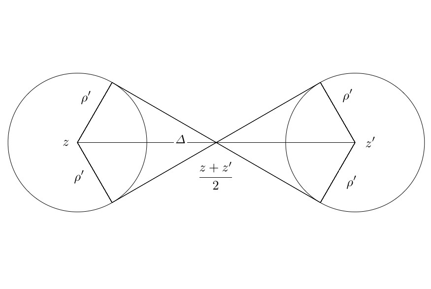
Figure 1:

The discs $D(z,\rho’)$ and $D(z’,\rho’)$ are from the proof of Lemma 1.

The parameter $\Delta=|z-z’|$ is used in Theorems 4.1 and 4.2.

Next apply it to a pair of nodes of the grid having centers $z$ and $z^{\prime}$, $\alpha=\frac{\pi}{8}$, and $\gamma=\frac{\pi}{4}$. Let the two nodes lie in the two discs $D(z,\rho^{\prime})$ and $D(z^{\prime},\rho^{\prime})$ for $\rho^{\prime}=\rho~{}\sqrt{2}$ and $|z-z^{\prime}|>2\rho^{\prime}$, and obtain

$$\frac{\rho^{\prime}}{|z-z^{\prime}|}-\frac{1}{6}\Big{(}\frac{\rho^{\prime}}{|z-z^{\prime}|}\Big{)}^{3}<\sin\Big{(}\frac{\rho^{\prime}}{|z-z^{\prime}|}\Big{)}<\frac{\rho^{\prime}}{|z-z^{\prime}|}.$$

Then the lemma implies the strict upper bound $\frac{4}{\pi}\frac{\rho^{\prime}}{|z-z^{\prime}|}$ on the probability $P$. Substitute $\rho^{\prime}=\rho~{}\sqrt{2}$ and obtain

$$P<\frac{4\rho\sqrt{2}}{\pi~{}|z-z^{\prime}|}.$$ (4)

Theorem 4.1

Let the grid of Algorithm 1 have $N_{\rho}$ nodes overall, $N_{\rho}\leq n^{2}$. Define the smallest superscribing disc for every node of a grid. Fix $\Delta>2\rho$ and call a node of the grid $\Delta$-isolated if the $\Delta$-neighborhood of its center contains no centers of any other node of the grid. Suppose that a rectangle of the third family intersects a fixed $\Delta$-isolated node. Then

(i) this rectangle intersects the smallest superscribing disc of another node of the grid with a probability less than $\frac{4\rho\sqrt{2}}{\pi\Delta}(N_{p}-1)$,

(ii) the probability that any rectangle of the third family intersects the smallest superscribing discs of at least two $\Delta$-isolated nodes is less than $\frac{2\rho\sqrt{2}}{\pi\Delta}(N_{p}-1)N_{p}$, and

(iii) if

$$\frac{2\rho\sqrt{2}}{\pi\Delta}(N_{p}-1)N_{p}\leq\epsilon,$$ (5)

then Algorithm 1 outputs the claimed set of the roots of a polynomial $p(x)$ with a probability more than $1-\epsilon$.

Proof

Apply bound (4) to the fixed node and obtain part (i). Apply bound (4) to all $(N_{p}-1)N_{p}/2$ pairs of distinct nodes of the grid and obtain part (ii). Substitute bound (5) and obtain part (iii).

Now correctness of the algorithm follows because every root of the polynomial $p(x)$ lies in some annulus of each of the three families.

4.3 Approximation of complex roots: complexity of performing Algorithm 1 and further comments

Remark 1

The estimates of Theorem 4.1 are pessimistic because, for any integer $k>1$, every $k$-tuple of nodes intersected by a single straight line contributes to the probability count of Theorem 4.1 just as much as a single pair of nodes, but we count the contribution of such a $k$-tuple as that of $(k-1)k/2$ pairs of nodes.

Theorem 4.2

Suppose that we are given the coefficients of a polynomial $p(x)$ of equation (1) and two constants $\rho$ and $\Delta$ such that $0<\rho<\Delta$. Apply Algorithm 1 for that fixed $\rho$. Then (i) with a probability of success estimated in Theorem 4.1, the algorithm approximates all roots in $\Delta$-isolated nodes within the error bound $\rho$, and (ii) the algorithm performs at the Boolean cost within the randomized cost bound of Corollary 1.”

Proof

We can readily verify both claims of the theorem as soon as we ensure as soon as we ensure that the Boolean complexity of Stage 3 of Algorithm 1 is within the claimed bound. To achieve this, apply a bisection process as follows. At first, for a fixed rectangle of the third family, determine whether it intersects any node of the grid below or any node of the grid above its mean node. If the answer is “yes” in both cases, then the rectangle must intersect more than one node of the grid. Otherwise discard about one half of the nodes of the grid and apply similar bisection process to the remaining nodes. Repeat such computation recursively.

Every recursive step either determines that the fixed rectangle intersects more than one node of the grid or discards about 50% of the remaining nodes of the grid. So in $O(\lg(n))$ recursive applications we determine whether the rectangle intersects only a single node of the grid or not.

Application of this process to every rectangle of the third family (made up of $n$ rectangles) requires only $O(n\lg(n))$ tests of the intersections of rectangles with a mean node in the set of the remaining nodes of the grid. Clearly the overall cost of these tests is dominated.

Remark 2

Suppose that we modify Algorithm 1 by collapsing every chain of $m$ pairwise overlapping or coinciding root radii intervals, for $m\leq n$, into a single interval that has a width at most $m\rho$ and by assigning multiplicity $m$ to this interval. Such extended root radius defines an annulus having multiplicity $m\geq 1$ and width in the range from $\rho$ to $m\rho$. Suppose that a pair of such new annuli of a vertical and horizontal families and the disc $D=D(0,r_{1}^{+})$ has multiplicity $m_{1}$ and $m_{2}$, respectively. Then the intersection of these two annuli defines a node of a new grid, to which we assign multiplicity $\min\{m_{1},m_{2}\}$, and then at Stage 3 of the modified algorithm an output node of multiplicity $m$ contains at most $m$ roots of the polynomial $p(x)$, each counted according to its multiplicity. The probability of success of the algorithm does not decrease and typically increases a little, although the estimation of the increase would be quite involved.

Remark 3

Suppose Algorithm 1 modified according to the previous remark outputs a node that cover an isolated root or an isolated cluster of the roots of an input polynomial $p(x)$. Then the algorithms of [K98], [PT14], [PT16] would compress the superscribing disc of this node at a nearly optimal Boolean cost.

Remark 4

We can decrease a little the precision of computing by applying the algorithm with a smaller value of $\eta$, although in that case our proof of Theorem 4.1 would be invalid, and the algorithm would become heuristic.

Remark 5

Suppose that we apply our algorithm as before, but fix an angle $\phi$ instead of choosing it at random in the range $[\pi/8,3\pi/8]$. Then for almost all such choices, the algorithm (at its Stage 4) would correctly determine at most $n$ nodes of the grid intersected by the rectangles-annuli of the third family, but finding any specific angle $\phi$ with this property deterministically would be costly because we would have to ensure that the angle of the real axis with neither of up to $(n^{2}-1)n^{2}/2$ straight lines passing through the $(n^{2}-1)n^{2}/2$ pairs of the nodes of the grid approximates $\phi$ closely. Clearly, this could require us to perform up to $(n^{2}-1)n^{2}/2$ flops.

5 Conclusions

Algorithm 1 approximates all the isolated single and multiple roots of a polynomial, and its modification of Remark 3 enables us to approximate also all the isolated root clusters. Having specified a modified node containing such a cluster, we can split out a factor $f(x)$ of the polynomial $p(x)$ whose root set is precisely this cluster. Based on the algorithms of [K98] or [PT16], we can approximate the factor $f(x)$ at a nearly optimal Boolean cost. Then we can work on root-finding separately for this factor and for the complementary factor $\frac{p(x)}{f(x)}$, both having degrees smaller than $n$ and possibly having better isolated roots.

We plan to work on enhancing the efficiency of this algorithm by means of its combination with various efficient techniques known for root-finding. In particular, the coefficient size of an input polynomial grows very fast in Dandelin’s root-squaring iterations, thus involving computations with high precision. The paper We can avoid this growth by applying the algrithm of [MZ01], which uses the tangential representation of the coefficients, but then the Boolean cost bound grows by a factor of $n$. So we are challenged to explore alternative techniques for root-radii approximations. We would be interested even in a heuristic algorithm, as long as it produces correct outputs for a large input class and performs the computations by using a small number of flops and a low precision.

Acknowledgements: Our work has been supported by NSF Grants CCF 1116736 and CCF 1563942 and PSC CUNY Awards 67699-00 45 and 68862–00 46.

References

- [B79] Bruno, A.D.: The Local Method of Nonlinear Analysis of Differential Equations. Nauka, Moscow (1979) (in Russian). English translation: Soviet Mathematics, Springer, Berlin (1989)
- [B96] Bini, D.: Numerical computation of polynomial zeros by means of Aberth’s method. Numerical Algorithms, 13, 179–200 (1996)
- [B98] Bruno, A.D.: Power Geometry in Algebraic and Differential Equations. Fizmatlit, Moscow (in Russian), English translation: North-Holland Mathematical Library, 57, Elsevier, Amsterdam (2000), also reprinted in 2005, ISBN: 0-444-50297
- [BF00] Bini, D. A., Fiorentino, G.: Design, analysis, and implementation of a multiprecision polynomial rootfinder. Numerical Algorithms, 23, 127–173 (2000)
- [BR14] Bini, D.A., Robol, L.: Solving secular and polynomial equations: a multiprecision algorithm. J. Computational and Applied Mathematics, 272, 276–292 (2014)
- [G72] Graham, R. l.: An efficient algorithm for determining the convex hull of a finite planar set. Information Processing Letters, 1, 132–133 (1972)
- [H59] Householder, A.S.: Dandelin, Lobachevskii, or Graeffe. Amer. Math. Monthly, 66, 464–466 (1959)
- [H74] Henrici, P.: Applied and Computational Complex Analysis. Wiley, New York (1974)
- [K98] Kirrinnis, P.: Partial fraction decomposition in and simultaneous Newton iteration for factorization in . Journal of Complexity, 14, 378–444 (1998)
- [MP13] McNamee, J.M., Pan, V.Y.: Numerical Methods for Roots of Polynomials. Part 2 (XXII + 718 pages), Elsevier (2013)
- [MZ01] Malajovich, G.,. Zubelli, J. P.: Tangent Graeffe iteration. Numerische Mathematik, 89(4), 749–782 (2001)
- [O40] Ostrowski, A. M.: Recherches sur la méthode de Graeffe et les zéros des polynomes et des series de Laurent. Acta Math., 72, 99–257 (1940)
- [P95] Pan, V.Y.: Optimal (up to polylog factors) sequential and parallel algorithms for approximating complex polynomial zeros. In: Proc. 27th Ann. ACM Symp. on Theory of Computing, pages 741–750. ACM Press, New York (1995)
- [P00] Pan, V.Y.: Approximating complex polynomial zeros: modified quadtree (Weyl’s) construction and improved Newton’s iteration. J. of Complexity, 16(1), 213–264 (2000)
- [P01] Pan, V.Y.: Structured Matrices and Polynomials: Unified Superfast Algorithms. Birkhäuser, Boston, and Springer, New York (2001)
- [P02] Pan, V.Y.: Univariate polynomials: nearly optimal algorithms for factorization and rootfinding. J. of Symbolic Computation, 33(5), 701–733 (2002). Proceedings version in ISSAC’2001, pages 253–267, ACM Press, New York (2001)
- [PT13] Pan, V.Y., Tsigaridas, E.P.: On the Boolean complexity of the real root refinement. In: Proceedings of the International Symposium on Symbolic and Algebraic Computation (ISSAC 2013), (M. Kauers editor), pages 299–306, Boston, MA, June 2013. ACM Press, New York (2013)
- [PT14] Pan, V.Y., Tsigaridas, E.P.: Accelerated approximation of the complex roots of a univariate polynomial. In: Proceedings the International Conference on Symbolic and Numeric Computation (SNC’2014), Shanghai, China, July 2014, pages 132–134. ACM Press, New York (2014). Also April 18, 2014, arXiv : 1404.4775 [math.NA]
- [PT15] Pan, V.Y., Tsigaridas, E.P.: Nearly optimal refinement of real roots of a univariate polynomial. J. of Symbolic Computation, in print.
- [PT16] Pan, V.Y., Tsigaridas, E.P.: Accelerated approximation of the complex roots and factors of a univariate polynomial. Theoretical Computer Science, Special Issue on Symbolic–Numerical Algorithms (Stephen Watt, Jan Verschelde, and Lihong Zhi, editors), in print.
- [PZ15] Pan, V.Y., Zhao, L.: Real root isolation by means of root radii approximation. In: Proceedings of the 17th International Workshop on Computer Algebra in Scientific Computing (CASC’2015), (V. P. Gerdt, V. Koepf, and E. V. Vorozhtsov, editors), Lecture Notes in Computer Science, 9301, 347–358, Springer, Heidelberg (2015).
- [S82] Schönhage, A.: The fundamental theorem of algebra in terms of computational complexity. Math. Department, Univ. Tübingen, Germany (1982)
- [VdS70] Van der Sluis, A.: Upper bounds on the roots of polynomials. Numerische Math., 15, 250–262 (1970)