2cm2cm2cm2cm

Overcoming the ill-posedness through discretization in vector tomography:
Reconstruction of irrotational vector fields

Technical (PhD Transfer) Report

January 2011

Student: Alexandra Koulouri
Supervisor: Prof. M. Petrou
Communications & Signal Processing Group

Department of Electrical & Electronics Engineering

Imperial College London

Chapter 1 Introduction

Vector field tomographic methods intend to reconstruct and visualize a vector field in a bounded domain by measuring line integrals of projections of this vector field.

In particular, we have to deal with an inverse problem of recovering a vector function from boundary measurements. As the majority of inverse problems, vector field method is ill posed in the continuous domain and therefore further assumptions, measurements and constraints should be imposed for the full vector field recovery. The reconstruction idea in the discrete domain relies on solving a numerical system of linear equations which derives from the approximation of the line integrals along lines which trace the bounded domain [30].

This report presents an extensive description of a vector field recovery method inspired by [30], elaborating on fundamental assumptions and the ill conditioning of the problem and defines the error bounds of the recovered solution. Such aspects are critical for future implementations of the method in practical applications like the inverse bioelectric field problem.

Moreover, the most interesting results from previous work on the tomographic methods related to ray and Radon transform are presented, including the basic theoretical foundation of the problem and various practical considerations.

1.1 Motivation

In the present project, the final goal is the implementation of a different approach for the EEG (Electroencephalography) analysis employing the proposed vector field method. Rather than estimating strengths or locations of the electric sources inside the brain, which is a very complicated task, a reconstruction of the corresponding static bioelectric field will be performed based on the line integral measurements. This static bioelectric field can be treated as an “effective” equivalent state of the brain at any given instant. Thus for instance, health conditions and specific pathologies (e.g. seizure disorder) may be recognized.

For this purpose, in the current report a robust mathematical and physical model and subsequently an efficient numerical implementation of the problem will be formulated. As a future stage, this theoretical and numerical formulations will be adapted to the real EEG problem with the help of experts and neuroscientists.

1.2 Report Structure

The rest of the report consists of four sections. The $2^{st}$ chapter is introductory and gives a brief description of the previously related work as well as the mathematical definition and theorems used by vector field tomographic methods. The $3^{rd}$ chapter gives an overview of the numerical vector field recovery method. Mathematical definitions, physical assumptions and conditions for the recovery of an irrotational vector field from line integral measurements without considering any boundary condition are described. Also, the approximation errors derived from the discretization of the line integrals and the a-prior error bounds are estimated. In the $4^{th}$ chapter, verification of the theoretical model by performing simulations as well as the practical adaptation of this model to the inverse bioelectric field problem using EEG measurements are described. Finally in the $5^{th}$ chapter, future work is discussed.

Chapter 2 Previous Work

In this chapter, we review several techniques that are important mathematical prerequisites for a better understanding of the vector field reconstruction problem. Moreover, an overview of the most prominent potential applications is presented.

2.1 Mathematical Preliminaries

The basic mathematical tools for the vector field problem formulation are presented in the following sections.

2.1.1 Formulation of Vector Field Tomography problem

The reconstruction of a scalar function $f(\textbf{n})$ from its line integrals or projections in a bounded domain is a well known problem. Today there are many practical and research applications in different fields such as biomedicine (e.g. MRI, CT), acoustic and seismic tomography which employ this method with great success and accuracy. However, there is a variety of other applications, like blood flow (velocity) in vessels or the diffusion tensor MRI problem where the estimation and the imaging of a vector field can be essential for the extraction of useful information. In these cases tomographic vector methods intend to reconstruct these fields from scalar measurements (projections) in a similar way to the scalar tomographic methods.

The mathematical formulation of the vector tomographic problem is given by the line integrals (projection measurements $I_{L}$)

$$I_{L}=\int_{L}\textbf{F}\cdot d\textbf{r}=\int\textbf{F}\cdot\hat{\textbf{r}}dr$$ (2.1)

where $\hat{\textbf{r}}$ is the unit vector in the direction of line L and F is the vector field to be recovered.

A different formulation for the projection measurement in $2D$ domain commonly used in bibliography involves the 1-D Dirac delta function such as

$$I_{L}=\int\int_{D}(F_{x}(x,y)\cos\phi+F_{y}(x,y)\sin\phi)\delta(x\sin\phi-y\cos\phi-\rho)dxdy$$ (2.2)

where $x\sin\phi-y\cos\phi=\rho$ is the line function with parameters $(\rho,\phi)$ defined as shown in figure 2.1 and $D$ is the bounded domain where $\textbf{F}(x,y)\neq 0$.

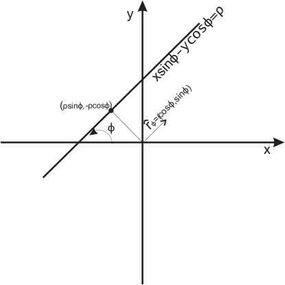
Figure 2.1: Line $L$ on $z$ plane with parameters $(\rho,\phi)$

where $0^{0}\leq\phi\leq 180^{0}$ and $\rho\,\in\,\Re$.

In general the vector tomographic problem is considered to be ill posed since F is defined by two or three components. However, with the application of certain constraints, restrictions and further assumptions there are ways to solve the problem.

2.1.2 Helmholtz decomposition

The Helmholtz decomposition [1] is a fundamental theorem of the vector calculus analysis as we shall see later.

It states that any vector F which is twice continuously differentiable and which, with its divergence and curl, vanishes faster than $1/r^{2}$ at infinity, can be expressed uniquely as the sum of a gradient and a curl as follows:

$$\textbf{F}=\textbf{F}_{I}+\textbf{F}_{S}\Rightarrow$$

$$\textbf{F}=-\nabla\Phi+\nabla\times\textbf{A}$$ (2.3)

The scalar function $\Phi$ is called the scalar potential and A is the vector potential which should satisfy $\nabla\cdot\textbf{A}=0$.

Since, $\nabla\times\textbf{F}_{I}=\nabla\times(\nabla\Phi)=0$, component $\textbf{F}_{I}$ is called irrotational or curl-free while $\textbf{F}_{S}$ is the solenoidal or divergence-free component as it satisfies $\nabla\textbf{F}_{S}=\nabla\cdot(\nabla\times\textbf{A})=0$.

In the case of a $2D$ vector field $\textbf{F}(x,y)$, the decomposition equation becomes

$$\textbf{F}=-\nabla\Phi+\nabla\times A_{z}(x,y)\hat{z}$$

.

2.1.3 Vectorial Ray Transform

In tomographic theory, the line integral 2.1 is called ray transform. This transform is closely related to the Radon transform [10] and coincides with it in two dimensions. In higher dimensions, the ray transform of a function is defined by integrating over lines rather than hyper-planes as the Radon transform.

In particular, for a bounded volume $V$ ($\textbf{F}=0$ outside $V$) and according to equation 2.1, the vectorial ray transform can be expressed as

$$\begin{split}I(\phi,\theta,\textbf{p})=&\int_{L(\phi,\theta,\textbf{p})}\textbf{F}\cdot\hat{\textbf{r}}_{\phi,\theta}dr=\\ =&\int_{L(\phi,\theta,\textbf{p})}F_{x}(x,y,z)\cos\phi\sin\theta dr\\ +&\int_{L(\phi,\theta,\textbf{p})}F_{y}(x,y,z)\sin\phi\sin\theta dr\\ +&\int_{L(\phi,\theta,\textbf{p})}F_{z}(x,y,z)\cos\theta dr\end{split}$$ (2.4)

where $F_{x}$, $F_{y}$ and $F_{z}$ are the components of vector F, $\phi$ and $\theta$ define the direction of the $\hat{\textbf{r}}_{\phi,\theta}$ unit vector along line $L(\theta,\phi,\textbf{p})$ as shown in figure 2.2 and $\textbf{p}=(x_{p},y_{p})$. Point p gives the coordinates of the line in the plane which passes through the origin of the axes and it is vertical to $\hat{\textbf{r}}_{\phi,\theta}$ (see fig. 2.2).

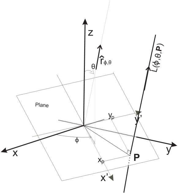
Figure 2.2: 3D ray transform geometry.

Consequently, the line integral 2.4 can be written as a volume integral using the appropriate Dirac delta functions. Thus we have

$$\begin{split}I(\phi,\theta,\textbf{p})&=\int\int\int_{V}F_{x}(x,y,z)\cos\phi\sin\theta\delta_{x_{p}}\delta_{y_{p}}dxdydz\\ &+\int\int\int_{V}F_{y}(x,y,z)\sin\phi\sin\theta\delta_{x_{p}}\delta_{y_{p}}dxdydz\\ &+\int\int\int_{V}F_{z}(x,y,z)\cos\theta\delta_{x_{p}}\delta_{y_{p}}dxdydz\end{split}$$ (2.5)

where

$$\delta_{y_{p}}=\delta(x\sin\phi-y\cos\phi-y_{p})$$

and

$$\delta_{x_{p}}=\delta(-x\cos\phi\cos\theta-y\sin\phi\cos\theta+z\sin\theta-x_{p})$$

In two dimensions, $\theta=\pi/2$ and $p$ is the signed distance of the line from the origin of the axes. Thus, equation 2.5 becomes

$$I(\phi,p)=\int\int_{D}(F_{x}(x,y)\cos\phi+F_{y}(x,y)\sin\phi)\delta(x\sin\phi-y\cos\phi-p)dxdy$$ (2.6)

and $\textbf{F}(x,y)=0$ outside D.

2.1.4 Central Slice Theorem

The solution to the inverse scalar ray transform is based on the central slice theorem (CST). CST states that the values of the $2D$ FT of scalar function $f(x,y)$ along a line with inclination angle $\phi$ are given by the $1D$ FT of its projection $I(\phi,p)$. This fact combined with the implementation of many practical algorithms (e.g. back-projection) gave rise to the development of accurate and robust reconstruction methods.

In the vectorial ray transform, the CST does not help us solve the problem. However, the formulation of the problem based on the CST is important for better understanding the theoretical approaches which will be described in the next section.

Let the Fourier Transform of $I(\phi,\theta,\textbf{p}=\{x_{p},y_{p}\})$ be

$$\widetilde{I}_{\phi,\theta}(k_{1},k_{2})=\int\int I(\phi,\theta,x_{p},y_{p})e^{-i(k_{1}x_{p}+k_{2}y_{p})}dx_{p}dy_{p}$$ (2.7)

Then according to equations 2.4 and 2.5 we obtain

$$\widetilde{I}_{\phi,\theta}(k_{1},k_{2})=\cos\phi\sin\theta\widetilde{F}_{x}(u,v,w)+\sin\phi\sin\theta\widetilde{F}_{y}(u,v,w)+\cos\theta\widetilde{F}_{z}(u,v,w)$$ (2.8)

where $\widetilde{F}_{x}$, $\widetilde{F}_{y}$ and $\widetilde{F}_{z}$ are the Fourier transforms of $F_{x}$, $F_{y}$ and $F_{z}$ respectively and $u=k_{1}\sin\phi-k_{2}\cos\phi\cos\theta$, $v=-k_{1}\cos\phi-k_{2}\sin\phi\cos\theta$ and $w=k_{2}\sin\theta$.

Applying the Helmholtz decomposition (eq. 2.3) we have

$$F_{x}(x,y,z)=\frac{\partial{A}_{z}}{\partial y}-\frac{\partial A_{y}}{\partial z}-\frac{\partial\Phi}{\partial x}$$

$$F_{y}(x,y,z)=-\frac{\partial{A}_{z}}{\partial x}+\frac{\partial A_{x}}{\partial z}-\frac{\partial\Phi}{\partial y}$$

$$F_{z}(x,y,z)=\frac{\partial{A}_{y}}{\partial x}-\frac{\partial A_{x}}{\partial y}-\frac{\partial\Phi}{\partial z}$$

Their Fourier transform leads to

$$\widetilde{F}_{x}(u,v,w)=iv\widetilde{A}_{z}(u,v,w)-iw\widetilde{A}_{y}(u,v,w)-iu\widetilde{\Phi}(u,v,w)$$

$$\widetilde{F}_{y}(u,v,w)=iw\widetilde{A}_{x}(u,v,w)-iu\widetilde{A}_{z}(u,v,w)-iv\widetilde{\Phi}(u,v,w)$$

$$\widetilde{F}_{z}(u,v,w)=iu\widetilde{A}_{y}(u,v,w)-iv\widetilde{A}_{x}(u,v,w)-iw\widetilde{\Phi}(u,v,w)$$

when A and $\Phi$ tend to zero on the volume boundaries.

Therefore the Fourier transform of the projection can be written as

$$\begin{split}\widetilde{I}_{\phi,\theta}(k_{1},k_{2})=&i(k_{1}\cos\phi\cos\theta+k_{2}\sin\phi)\widetilde{A}_{x}\\ +&i(k_{1}\sin\phi\cos\theta-k_{2}\cos\phi)\widetilde{A}_{y}-ik_{1}\sin\theta\widetilde{A}_{z}\end{split}$$ (2.9)

For the two dimensional case, $\theta=\pi/2$ and $k_{2}=0$ (as we have only one variable)

$$\widetilde{I}_{\phi}(k)=ik\widetilde{A}_{z}(k\cos\phi,k\sin\phi)$$ (2.10)

It is important to be mentioned that irrotational component $\Phi$ vanishes in equations 2.9 and 2.10.

2.2 Theoretical Approaches

The most important theoretical and mathematical studies of the vector field tomographic reconstruction from boundary measurements, as well as the feasibility of this formulation to yield unique solutions under certain constraints, were investigated only by a small group of the research community working in this field. Norton [26], Baun and Haucks [2] and Prince [31], [28] gave a step by step mathematical solution to the problem on bounded domains employing the Radon transform theory. In the following subsection, a description of their ideas and their methods is presented.

2.2.1 Tomographic Vector Field Methods

Norton in [26] and [27] was the first who defined the full mathematical formulation of the two dimensional problem. Norton proved that only the solenoidal component of a vector field F on a $D$ bounded domain can be uniquely reconstructed from its line integrals. Moreover, he showed that when the field F is divergenceless i.e. there are no sources or sinks in $D$, then both components can be recovered.

In particular, assuming a bounded vector field F, i.e $\textbf{F}=0$ outside a region $D$ which satisfies the homogeneous Neumann conditions on $\partial{D}$ (on the field’s boundaries), he produced equation 2.10 applying Helmzoltz decomposition (eq. 2.3) and the Central Slice Theorem (eq.2.7). Therefore, he proved that only the solenoidal component $\nabla\times\textbf{A}$ can be determined.

Furthermore, in [26] he demonstrated that when vector field F is divergenceless ($\nabla\textbf{F}=0$), then irrotational component $\Phi$ can be recovered.

From the divergence of the decomposition (eq. 2.3) we obtain

$$\nabla\textbf{F}=-\nabla(\nabla\Phi)+\nabla(\nabla\times\textbf{A})\Rightarrow\nabla^{2}\Phi=0$$

Thus, Norton was led to the Laplacian equation $\nabla^{2}\Phi=0$. The solution of the Laplacian equation gives the irrotational component and a full reconstruction of the field is possible. Norton employed Green’s theorem and F’s boundary values for the estimation of $\Phi$ on $D$.

Later Braun and Hauck [2] showed that the projection of the orthogonal components of the vector function (transverse projection measurement) leads to the reconstruction of the irrotational component $\nabla\Phi$. So, they proposed that for the full $2D$ field reconstruction, a longitudinal and a transverse measurement are needed

$$I_{\parallel}=\int\textbf{F}\cdot\hat{\textbf{r}}dr\;\;\mbox{and}\;\;I_{\perp}=\int\textbf{F}\cdot\hat{\textbf{r}}_{\perp}dr$$

where $\hat{\textbf{r}}$ is the unit vector along the line and $\hat{\textbf{r}}_{\perp}$ is the unit vector orthogonal to the line.

Moreover, they examined the problem for non-homogeneous boundary conditions. In that case, the irrotational and solenoidal decomposition is not unique and they proposed to decompose the vector into three components: the homogeneous irrotational, the homogeneous solenoidal and the harmonic with its curl and divergence being zero. They verified their method carrying out fluid flow estimation experiments. With this method there is no need to assume that there are no sources inside the domain. However, the difficulty of taking transversal measurements as it was mention in [27] makes the method quite impractical, especially for Doppler back scattering methods.

Prince [31] and Prince and Osman [28] extended the previous method to $3$ dimensions, reconstructing both the solenoidal and the irrotational components of F from the inverse $3D$ Radon transform. Actually they evolved the Braun-Hauck’s method by defining a more general inner product measurement which was called probe transform and it was expressed as

$$G^{\textbf{p}}(\textbf{a},\rho)=\int_{\Re^{3}}\textbf{p}(\textbf{a},\rho)\cdot\textbf{F}(x,y,z)\delta(xa_{x}+ya_{y}+za_{z}-\rho)dxdydz$$ (2.11)

where p is the so-called vector probe, $\rho$ the distance of the projection plane from the origin and $\textbf{a}=(a_{x},a_{y},a_{z})$ the normal vector to the plane.

With the application of Helmholtz decomposition for homogeneous field’s boundaries (eq. 2.3) and the Cental Slice Theorem, equation 2.11 becomes

$$\widetilde{G}^{\textbf{p}}(\textbf{a},k)=(j2\pi k)\textbf{p(a)}\cdot[\Phi(k\textbf{a})\textbf{a}+\textbf{a}\times A(k\textbf{a})]$$

Therefore, if p is orthogonal to a then the irrotational component is eliminated, while when p is parallel to a then the solenoidal component vanishes. On this basic principle Prince and Osman based their model for the reconstruction of a $3D$ vector field.

2.3 Proposed Applications

A plethora of different applications have been proposed in the area of vector field tomography. Some of the earlier studies by Johnson et al.[19] and Johnson [15] were concerned with the reconstruction of the flow of a fluid by applying numerical techniques (iterative algebraic reconstruction techniques). Johnson et al. [19] used ultrasound measurements (acoustic rays) to reconstruct the velocity field of blood vessels. Later, other applications like optical polarization tomography [11] for the estimation of electric field in a Kerr material and oceanographic tomography [32] were also reported. In Kramar’s thesis [21] a vector field method for the estimation of the magnetic field of the sun’s coronal is presented, giving interesting results.

Moreover, in vector field literature there are many other proposed applications in the area of Doppler back scattering, Optical tomography, Photoelasticity and Nuclear Magnetic Resonance Plasma physics [4]. However, there are only a few practical or commercial applications in this field.

2.3.1 Vector Field Reconstruction and Biomedical Imaging

Vector field tomography has not received much attention in the area of medical applications. There are only a few papers [29, 22, 12, 13, 6, 33] and one PhD thesis [14] which present relevant methods. The main area of research according to these papers are Doppler back scattering for blood flow estimation, although till now there are only simulations and theoretical formulations without performing any real experiment or employing real data.

Moreover, the Lawrence Berkeley National Laboratory [4] has developed many tomographic mathematical tools and algorithms for medical imaging issues. As it is mention in [4], their work has focused mainly on the implementation of algorithms for the reconstruction of the $3D$ diffusion tensor field from MRI tensor projections and iterative algorithms for solving the non-linear diffusion tensor MRI problem.

2.4 Summary

Study of previous work indicates that the vector field tomography has practical potential. Till now much of the work was devoted to the theoretical development and formulation of the problem. Moreover it is clear that the acquisition of the measurements and the performance of real experiments are quite difficult tasks and a multidisciplinary collaboration is required.

Chapter 3 Vector Field Recovery Method: a Linear Inverse Problem

In the previous chapter, an extended description of the mathematical expression of the vector field tomographic problem in ray and Radon transform sense was presented. A different approach for vector field recovery method stemming from the numerical inverse problems theory will be considered here.

The numerical solution of an inverse problem requires the definition of a set of equations mathematically adapted to the physical properties of the problem, subsequently, the design of the geometrical model where these equations operate and finally the discretization of the equations to form a numerical system such as the approximated solution to be as close as possible to the real solution of the model.

So, the vector field recovery problem can be considered as an inverse problem which can be formulated as an operator equation of the form

$$K\textbf{x}=y$$

with $K$ being a linear operator between spaces $X$ and $Y$ over the field $\Re$ and where the geometrical and numerical models are designed according to the topological and error approximation requirements of the problem.

The current method is based on the estimation of a vector field from the line integrals (projection measurements) in an unbounded domain. Thus, $K$ operator is an integral operator and the vector field recovery method relies on solving a set of linear equations which derives from a set of numerically approximated line integrals which trace a bounded domain $\Omega$, and are expressed as

$$\int_{L}\textbf{E}\cdot d\textbf{r}=\Phi(\textbf{a})-\Phi(\textbf{b})$$

where E is the irrotational vector field, $d\textbf{r}=\hat{\textbf{r}}dr$ with $\hat{\textbf{r}}$ the unit vector along line $L$ and $\Phi$ gives the boundary measurements at starting point a and endpoint b.

The initial idea was put forward in [30] where it was shown that there is potential for a vector field to be recovered in a finite number of points from boundary measurements. However, this initial idea followed an intuitive approach to the problem as it lacked the necessary conditions and assumptions about the recovered field and the formulation of the equations. Moreover, there was no clear and robust proof about the well or ill posedness of this inverse problem.

Therefore, in the rest of this text:

• the necessary preconditions and assumptions are defined such as the mathematical formulation of the problem fits the physical vector field properties as closely as possible;

• an extended description of the vector field method employing the line integral formulation is given;

• the ill posedness of the vector field method in the continuous domain is investigated and we show that the number of independent equations which stem from the problem’s formulation give a final numerical system which is nearly rank deficient (ill conditioned);

• the approximation and discretization errors resulted by the numerical implementation of the problem are formulated. Finally, the solution error of the numerical system is estimated and the conditions under which this error is bounded are presented, revealing that the discretization is a way of “self-regularization” of this ill conditioned inverse problem.

3.1 Preconditions and Assumptions

Field E is assumed bounded and continuous in a domain $\Omega$, bandlimited, irrotational and quasi-static.

In particular, the quasi-static condition implies that the field behaves, at any instance, as if it is stationary. Moreover, the field is considered irrotational and satisfies $\nabla\times\textbf{E}=0$ and thus it can be represented by the gradient of a scalar function $\Phi$. So, $\textbf{E}=-\nabla\Phi$ in a simply connected region (Poincare’s Theorem [1]). Consequently, the gradient theorem gives

$$\int_{c}\textbf{E}\cdot d\textbf{c}=\int_{c}-\nabla\Phi d\textbf{c}=\Phi(\textbf{a})-\Phi(\textbf{b})$$ (3.1)

which will be the model equation of our problem and implies that the line integral of E along any curve $c$ is path-independent.

The irrotational property $\nabla\times{\textbf{E}}=0$ in integral form can be expressed by applying the well-known Stokes’ theorem (curl-theorem) which relates the surface integral of the curl of a vector field over a surface $S$ in Euclidean $3D$ space to the line integral of the vector field over its boundary $\partial{S}$ such as

$$\int_{S}\nabla\times\textbf{E}d\textbf{S}=\int_{\partial{S}}\textbf{E}\cdot d\textbf{c}$$

For an irrotational field obviously

$$\int_{\partial{S}}\textbf{E}\cdot d\textbf{c}=0$$ (3.2)

So, the path integral of E over a closed curve (path) is equal to zero.

Finally, vector field E is band limited, $\int\int_{|\Omega|}\|\textbf{E}\|dxdy<\infty$ and continuous in $\Omega$ thus is can be expanded in Fourier Series as

$$\textbf{E}(x,y)=\sum_{\textbf{k}}\textbf{e}_{k}e^{i\textbf{k}\langle x,y\rangle}+\bar{\textbf{e}}_{k}e^{-i\textbf{k}\langle x,y\rangle}$$

where $\textbf{k}=(n_{x},n_{y})$ with $n_{x},n_{y}=0,\pm 1,\pm 2\dots$.

As the physical and mathematical properties of the vector field have been defined, the mathematical and numerical formulation of the problem will be explained in the following section.

3.2 Methodology

3.2.1 Mathematical Modeling

The formulation of the method is based on the idea in [8] and [30] to approximately reconstruct a vector field E at a finite number of points when a sufficiently large number of line integrals $I_{L_{k}}$ along lines which trace the bounded domain, are known. The model equation for the recovery of an irrotational field inside a bounded convex domain $\Omega$ is given by

$$I_{L_{k}}=\int_{L_{k}}\textbf{E}\cdot d\textbf{r}$$ (3.3)

where line $L_{k}$ traces the bounded domain and intersects it in two points. As the field is irrotational, the line integral is $I_{L_{k}}=\Phi(\textbf{a}_{k})-\Phi(\textbf{b}_{k})$ where $\Phi$ are the boundary values at the intersection points $\textbf{a}_{k}$ and $\textbf{b}_{k}$ with domain $\Omega$. So, a set of linear equations 3.3 can be acquired for a finite number of known values $\Phi$ on the boundaries of $\Omega$.

3.2.2 Geometric Model

As the model equations have been defined, the next step is the geometric model generation. Generally, the geometric model is a discrete domain of specific shape where the model equations are valid. For instance, if the line integral equations (model equations) were employed for field recovery from scalp potential recordings (e.g. EEG), then the geometric model would be a $3D$ mesh with scalp shape.

In our initial approach for the evaluation of the method, a simple geometric model was designed as described in [30]. In particular, a discrete version of a $2D$ continuous square domain $\Omega=:\{(x,y)\in[-U,U]^{2}\}$ (fig.3.1) was defined using elements of constant size $[P\times P]$ called cells or tiles and $N=U/P$.

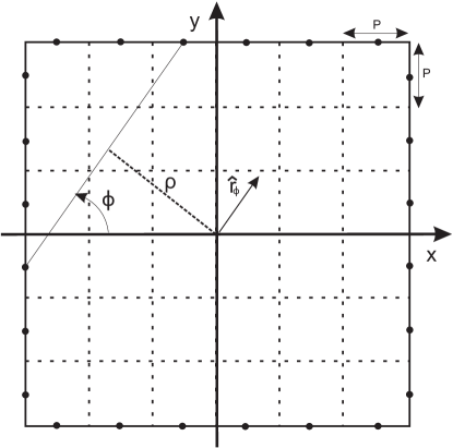
Figure 3.1: A line $L(\phi,\rho)$ of integration on a square discrete domain where $\phi$ is the counterclockwise angle between the positive $x$ axis and the line and $\rho$ the signed distance of the line from the origin.

The goal was to recover the field in each cell solving a numerical system of a discretized version of model equations 3.3. The number and the positions of the tracing lines $L_{k}$ in the bounded domain were defined by pairs of sensors (boundary measurements) which were placed in the middle of the boundary edges of all boundary cell (fig.3.1). Each tracing line connected a pair of sensors which did not belong to the same side of the square domain and thus for a $N=U/P$ number of edge cells or $N$ sensors in each side of the domain, the connected pairs led to $6N^{2}$ model equations (line integrals). The domain had $N\times N$ cells and the $2D$ vector field had two components. Thus the number of unknowns (value of each cell) was $2[N\times N]$ and the number of equations was $6N^{2}$ .

3.2.3 Numerical Implementation

For the numerical implementation of the method, the line integral 3.3 was approximated using the Riemann’s sum. Thus,

$$I_{L_{k}}\approx\sum_{(x_{m},y_{m})\in L_{k}}\textbf{E}(x_{m},y_{m})\cdot\hat{\textbf{r}}_{\phi}\Delta r$$ (3.4)

where $\textbf{E}(x_{m},y_{m})$ are the unknown vector values at sampling points $(x_{m},y_{m})$ along line $L(\phi,\rho)=\{(x,y)|\,x\sin\phi-y\cos\phi=\rho\}$ with $0^{0}\leq\phi\leq 180^{0}$ and $\rho\in\Re$ and $\hat{\textbf{r}}_{\phi}\Delta r=(\cos\phi\hat{\textbf{x}}+\sin\phi\hat{\textbf{y}})\Delta r$ (fig.3.1).

For the numerical approximation, the samples $\textbf{E}(x_{m},y_{m})$ are assigned to values $\textbf{E}[i,j]=(e_{x}[i,j],e_{y}[i,j])$ based on an interpolation scheme. The simple case of the nearest neighbor approximation in a $2D$ square domain $[-U,U]^{2}$ leads to $i=\lceil\frac{x_{m}+U}{P}\rceil$ and $j=\lceil{\frac{y_{m}+U}{P}}\rceil$.

Finally, all the approximated line integrals give a set of algebraic equations which can be represented by

$$\textbf{b}=\textbf{A}\textbf{x}$$ (3.5)

where x contains the unknown vector field components in finite points with index $u$, b is the column vector with the measured values of the line integrals $I_{L_{k}}$. The elements of the transfer matrix A, $a_{k,u}$ represent the weight of projection of the unknown element $u$ on the $I_{L_{k}}$. For the case of a discrete square domain as it was described in subsection 3.2.2, the $4N$ sensors around the boundaries give $6N^{2}$ equations and as the number of the unknowns is $2N^{2}$, at first sight we conclude that we deal with an over-determined system.

3.3 Ill Posedness and Ill Conditioning of the Inverse problem

If we ignore the physical properties of the field, the reconstruction formulation described in the subsections 3.2.2 and 3.2.3 seems correct and robust as the system 3.5 of algebraic equations is over-determined and thus with the least square method, the problem can be solved. However, the majority of the inverse problems are typically ill-posed.

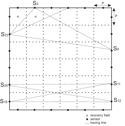
Figure 3.2: Tracing lines in the discrete domain which create closed-paths

In the current problem, the irrotational assumption of the field implies that a line integral along a closed path is zero. More precisely, taking all pairs of sensors which do not belong to the same side we obtain tracing lines which create closed paths (fig. 3.2). Particulary, when the tracing lines $L_{1},L_{2}\dots$ form a closed curve, according to equations 3.2 and 3.3 we obtain

$$I_{L_{1}}+I_{L_{2}}+\dots+I_{L_{n}}=0$$ (3.6)

or

$$-I_{L_{1}}=I_{L_{2}}+\dots+I_{L_{n}}$$

This indicates that a line integral can be expressed as a linear combination of other line integrals and thus we have linearly dependent equations $I_{L_{k}}$. For instance, in figure 3.2 the lines which connect sensors S₂, S₉ and S₂₃ create a closed loop and thus for equations (line integrals) $I_{L_{2-9}}$, $I_{L_{9-23}}$ and $I_{L_{23-2}}$ we have

$$I_{L_{2-9}}+I_{L_{9-23}}+I_{L_{23-2}} =$$

$$=\int_{{L_{2-9}}}\textbf{E}\cdot d\textbf{r}+\int_{{L_{9-23}}}\textbf{E}\cdot d\textbf{r}+ \int_{{L_{23-2}}}\textbf{E}d\textbf{r}=$$

$$=\int_{{L_{2-2}}}\textbf{E}\cdot d\textbf{r} =0$$

Therefore, only two equations can be assumed independent since any one of the three can be expressed as a linear combination of the other two equations.

The linear dependencies are quite significant in the continuous domain. On the other hand, in the discrete domain, where the integral is approximated by a summation, the dependencies are not so obvious as the accuracy of the continuous domain is lacking. Thus, taking Riemann’s summation (eq.3.4), leads to sums of equations close to zero

$$I_{L_{1}}+I_{L_{2}}+\dots+I_{L_{n}}\approx 0$$

If the accuracy improves, i.e rather than applying nearest neighbor approximation, a different interpolation scheme like bilinear, cubic or more sophisticated techniques e.g. finite elements and a grid refinement of the bounded domain, can lead to more obvious equation dependencies.

One important task is the examination of the stability of the solution of linear system 3.5 i.e. to check whether the independent equations are enough to give a unique solution and whether matrix A has full rank.

Ill Conditioning: Number of Independent Equations

The number of independent equations is important for the solution of the problem since in the case that this number is less than the unknowns, the system is under-determined and different mathematical tools are needed.

In order to define the number of independent equation, we have to exclude tracing lines which “close” paths such as making sure that any line starting from one sensor does not end up to the same sensor. The number of independent equations can be defined based on the fundamental properties of graph theory [5].

More specifically, we assume that the $4N$ sensors along the boundary of the square domain are the “vertices” of a graph G and that the lines which connect two sensors are the G graph’s “edges”. The main property that this graph should satisfy is that any two “vertices” are linked by a unique path or in other words that the graph should be connected and without cycles. According to graph theory, a “tree” is a undirected simple graph G that satisfies the previous condition.

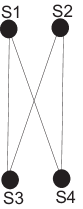
Figure 3.3: Graph G which is not acyclic. If we extract one edge then it becomes a tree.

Moreover, it is known that a connected, undirected, acyclic graph with $N$ “vertices” has $N-1$ “edges”. Therefore in a $2D$ square domain (subsection 3.2.2) with $4N$ sensors along the boundaries, the maximum number of tracing lines in order to avoid loops is $4N-1$ and so the number of independent equations (independent line integrals) is $4(N-1)$. In all, the system of equations may have at most $4N-1$ independent equations. Obviously, for a system with $2N^{2}$ unknowns, the $4(N-1)$ equations lead to an under-determined case.

As a result, the transfer matrix A of system 3.5 approximates a rank-deficient matrix i.e. there are nearly linearly dependent lines and the linear system may be inconsistent and severely ill conditioned.

3.3.1 Ill Conditioning Indicators

Generally speaking, the ill posedness technically applies to continuous problems. The discrete version of an ill posed problem may or may not be severely ill conditioned.

The discrete approximation will behave similarly to the continuous case as the accuracy of the approximation increases. With a “rough” approximation scheme and coarse discretization of the bounded domain, the linear dependencies of the equations are eliminated and transfer matrix A of system 3.5 is not rank deficient.

The condition number of transfer matrix A (system 3.5) and the magnitude of the singular values of A are reliable indicators of how close to rank deficiency and consequently to ill conditioning the numerical system is. For the case where a bounded domain $\Omega:\{(x,y)\rightarrow[-5.5,5.5]^{2}\subset\Re^{2}\}$ is discretized employing cells of size $P\times P=1\times 1$, and there are $4\times U/P=4\times N=121$ sensors along the boundaries (see subsection 3.2.2), $6N^{2}=726$ equations and the field is created by a single charge in position $(-19,19)$ on the z-plane as in [30], the condition number is $84$, which is not so large in order to deal with a severely ill-conditioned system. Moreover, the simulation results, which will be presented in the next chapter, show that the estimated solution is not far from the real one.

So, under certain conditions, system 3.5 which was derived from the numerical approximation of the line-integral can give acceptable results and the discretization process can be assumed as a kind of “self-regularization” (regularization by discretization) of the continuous ill posed problem.

The aim of the work presented next is the mathematical definition of the numerical errors due to the line-integrals approximations and how these errors are related with the ill conditioning of the linear system 3.5 defining an upper error bound of the system’s numerical solution.

3.4 Approximation Errors

For the numerical solution of a line integral system, one has to discretize the continuous problem and reduce it to a finite system of linear equations. The discretization process introduces approximation and rounding errors to the set of line integrals (model equations 3.3) which can be interpreted as perturbations. First, the mathematical formulation and nature of these errors will be described in the following analysis. Subsequently, the error of the numerical solution will be estimated.

3.4.1 Description and Derivation of the Approximation Errors

The estimation of the line integral (eq.3.3) in a $2D$ domain is given by Riemmann’s integral

$$I_{L_{\rho,\phi}}=\lim_{\max\{\Delta r_{k}\}\rightarrow 0}\sum_{k}\textbf{E}(x_{k},y_{k})\cdot\hat{\textbf{r}}_{\phi}\Delta r_{k}$$ (3.7)

where $(x_{k},y_{k})$ are the coordinates of the samples $\textbf{E}(x_{k},y_{k})$ of the field along line $L_{\rho,\phi}=\{(x,y)|x\sin\phi-y\cos\phi=\rho\}$ $\in\Omega$ with $\hat{\textbf{r}}_{\phi}=(\cos\phi,\sin\phi)$ the unit vector in the direction of the line (fig.3.1) and $\Delta r_{k}$ the sampling step.

The coordinates of the samples are $x_{k}=x_{k-1}+\Delta r_{k}\cos\phi$ and $y_{k}=y_{k-1}+\Delta r_{k}\sin\phi$ such as $(x_{k},y_{k})\in\Omega$.

Substituting E with its vector components $(e_{x},e_{y})$, equation 3.7 is expressed as

$$I_{L_{\rho,\phi}}=\lim_{\max\{\Delta r_{k}\}\rightarrow 0}\sum_{k}\{e_{x}(x_{k},y_{k})\cos\phi\Delta r_{k}+e_{y}(x_{k},y_{k})\sin\phi\Delta r_{k}\}$$ (3.8)

The numerical treatment of the problem is based on the assignment of each sample $\textbf{E}(x_{k},y_{k})$ to a value $\textbf{E}[i,j]$ of an element $[i,j]$ of the discrete domain. This assignment is actually a quantization process or “mapping” of the vector field samples to a finite set of possible discrete values (fig.3.4).

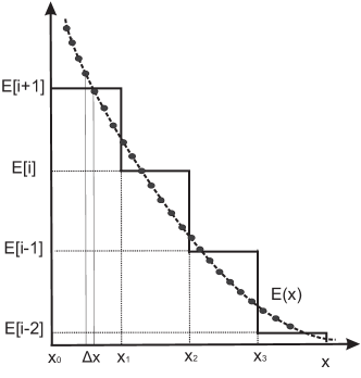
Figure 3.4: 1D equivalent representation for the assignment of the samples of field E to the middle cell values (quantization process). In the current representation, the samples of $E(x)$ are assigned to $E[i]$ values, where $\Delta x$ is the sampling step.

So, each sample $\textbf{E}(x_{k},y_{k})$ is the sum of $\textbf{E}[i,j]$ plus an error vector $\delta\textbf{E}(x_{k},y_{k})$. This can be expressed as

$$e_{x}(x_{k},y_{k})=e_{x}[i,j]+\delta e_{x}(x_{k},y_{k})$$ (3.9)

or briefly as

$$e_{x}^{k}=e_{x}[i,j]+\delta e_{x}^{k}$$

Similarly, the y-component is

$$e_{y}^{k}=e_{y}[i,j]+\delta e_{y}^{k}$$

Let us assume that there is a line segment $\Delta L_{ij}\subseteq L_{\rho,\phi}$ with length $\|\Delta L_{ij}\|$ which lies on element(cell) $[i,j]$ as in figure 3.5. Moreover, considering the sampling step to be constant $\Delta r_{k}=\Delta r$ and $N_{ij}$ the number of samples $\textbf{E}^{k}=(e_{x}^{k},e_{y}^{k})$ in $\Delta L_{ij}$, Riemann’s sum along segment $\Delta L_{ij}$ is

$$\begin{split}I_{\Delta L_{ij},\rho,\phi}=&\sum_{(e_{x}^{k},e_{y}^{k})\in\Delta L_{ij}}\{e_{x}^{k}\cos\phi\Delta r+e_{y}^{k}\sin\phi\Delta r\}=\\ =&\sum_{(e_{x}^{k},e_{y}^{k})\in\Delta L_{ij}}\left\{(e_{x}[i,j]+\delta e_{x}^{k})\cos\phi\Delta r+\left(e_{y}[i,j]+\delta e_{y}^{k}\right)\sin\phi\Delta r\right\}=\\ =&\left(N_{ij}e_{x}[i,j]+\sum_{k}\delta e_{x}^{k}\right)\cos\phi\Delta r+\left(N_{ij}e_{y}[i,j]+\sum_{k}\delta e_{y}^{k}\right)\sin\phi\Delta r\end{split}$$ (3.10)

Where $N_{ij}\in\aleph$ is the number of samples of $\Delta L_{ij}\subseteq L_{\rho,\phi}$ and segment $\Delta L_{ij}$ lies inside element $[i,j]$ of the discrete domain.

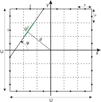
Figure 3.5: Segment $\Delta L_{ij}$ of line $L$ which lies inside element $[i,j]$ in a $2D$ square domain.

The error vector caused by the discretization process in an element $[i,j]$ is defined according to

$$(\delta\tilde{e}_{x}[i,j],\delta\tilde{e}_{y}[i,j])=\left(\sum_{k=N_{1}}^{N_{2}}\delta e_{x}^{k},\sum_{k=N_{1}}^{N_{2}}\delta e_{y}^{k}\right)$$ (3.11)

where $N_{2}-N_{1}+1=N_{ij}$ is the number of samples along $\|\Delta L_{ij}\|$.

The line integral (eq.3.8) can be represented as a sum of line integrals (eq.3.10) along segments $\Delta L_{ij}\subseteq L_{\rho,\phi}$.
Thus,

$$\begin{split}I_{L_{\rho,\phi}}=&\lim_{\Delta r\rightarrow 0}\sum_{\Delta L_{ij}}I_{\Delta L_{ij},\rho,\phi}=\\ =&\lim_{\Delta r\rightarrow 0}\sum_{\Delta L_{ij}}\sum_{\underset{\in\,\,\Delta L_{i,j}}{(e_{x}^{k},e_{y}^{k})}}\{e_{x}^{k}\cos\phi\Delta r+e_{y}^{k}\sin\phi\Delta r\}=\\ =&\lim_{\Delta r\rightarrow 0}\sum_{\Delta L_{ij}}\left\{\left(N_{ij}e_{x}[i,j]+\delta\tilde{e}_{x}[i,j]\right)\cos\phi\Delta r+\left(N_{ij}e_{y}[i,j]+\delta\tilde{e}_{y}[i,j]\right)\sin\phi\Delta r\right\}\end{split}$$ (3.12)

For simplicity, in the following equations indices $i$ and $j$ are substituted by a single index $m$.

So equation 3.12 becomes

$$I_{L_{\rho,\phi}}=\lim_{\Delta r\rightarrow 0}\sum_{\Delta L_{m}}\left\{(N_{m}e_{x}[m]+\delta\tilde{e}_{x}[m])\cos\phi\Delta r+(N_{m}e_{y}[m]+\delta\tilde{e}_{y}[m])\sin\phi\Delta r\right\}$$ (3.13)

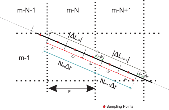
Figure 3.6: The sampling error $\varepsilon_{m}$ in element $[m]$ is less than zero as it was defined by $N_{m}\Delta r=\|\Delta L_{m}\|-\varepsilon_{m}\Delta r$ while in element $[m+1]$, $\varepsilon_{m+1}>0$.

The quantization error term due to the discretization process is defined as

$$\delta\tilde{E}=\lim_{\Delta r\rightarrow 0}\sum_{\Delta L_{m}}\left(\delta\tilde{e}_{x}[m]\cos\phi\Delta r+\delta\tilde{e}_{y}[m]\sin\phi\Delta r\right)$$ (3.14)

Thus, equation 3.13 becomes

$$I_{L_{\rho,\phi}}=\lim_{\Delta r\rightarrow 0}\sum_{\Delta L_{m}}\left\{N_{m}\Delta r(e_{x}[m]\cos\phi+e_{y}[m]\sin\phi)\right\}+\delta\tilde{E}$$ (3.15)

Sampling step $\Delta r$ is finite and $\min\{\|\Delta L_{m}\|\}\gg\Delta r>0$. Term $N_{m}\Delta r$ represents the length of a segment of line $L_{\rho,\phi}$ which “corresponds” to element $[m]$, where $N_{m}$ is the number of samples in element $[m]$ (fig.3.6). As the sampling step is $\Delta r\gg 0$, $N_{m}\Delta r\neq\|\Delta L_{m}\|$ as shown in figure 3.6. Thus, $N_{m}\Delta r=\|\Delta L_{m}\|-\varepsilon_{m}\Delta r$ with $|\varepsilon_{m}|<1$ being a sampling error coefficient.

The length of line $L_{\rho,\phi}$ is

$$\|L_{\rho,\phi}\|=\sum_{m}N_{m}\Delta r=\sum_{m}(\|\Delta L_{m}\|-\varepsilon_{m}\Delta r)=\sum_{m}\|\Delta L_{m}\|\,\,\,\mbox{and}\,\,\,\sum_{m}\varepsilon_{m}\Delta r=0.$$

Therefore, equation 3.15 is equal to

$$\begin{split}I_{L_{\rho,\phi}}=&\lim_{\Delta r\rightarrow 0}\sum_{\Delta L_{m}}\left\{(\|\Delta L_{m}\|-\varepsilon_{m}\Delta r)(e_{x}[m]\cos\phi+e_{y}[m]\sin\phi)\right\}+\delta\tilde{E}=\\ =&\sum_{\Delta L_{m}}\left\{\|\Delta L_{m}\|(e_{x}[m]\cos\phi+e_{y}[m]\sin\phi)\right\}+\delta\tilde{E}\end{split}$$

Finally, the line integral $I_{L_{\rho,\phi}}$ can be expressed as the sum of two terms, one which is the discretization process term $\sum_{\Delta L_{m}}\left\{\|\Delta L_{m}\|(e_{x}[m]\cos\phi+e_{y}[m]\sin\phi)\right\}$ and another which is error term $\delta\tilde{E}$ resulted by the discretization.

So,

$$I_{L_{\rho,\phi}}=\sum_{\Delta L_{m}}\left\{\|\Delta L_{m}\|(e_{x}[m]\cos\phi+e_{y}[m]\sin\phi)\right\}+\delta\tilde{E}$$ (3.16)

For the computational estimation of the line integrals, a finite number $N$ of samples $\textbf{E}(x_{k},y_{k})$ along line $L_{\rho,\phi}$ are assigned to the discrete values $\textbf{E}[m]$ based on an interpolation scheme (e.g. “rough” nearest neighbor). Thus, the approximated line integral equation has the form

$$\begin{split}\tilde{I}_{L_{\rho,\phi}}=&\sum_{\Delta L_{m}}\left\{N_{m}\Delta r(e_{x}[m]\cos\phi+e_{y}[m]\sin\phi)\right\}=\\ =&\sum_{\Delta L_{m}}\{(\|\Delta L_{m}\|-\varepsilon_{m}\Delta r)(e_{x}[m]\cos\phi+e_{y}[m]\sin\phi)\}=\\ =&\sum_{\Delta L_{m}}\{\|\Delta L_{m}\|(e_{x}[m]\cos\phi+e_{y}[m]\sin\phi)\}-\varepsilon(\Delta r)\end{split}$$ (3.17)

Where

$$\varepsilon(\Delta r)=\sum_{\Delta L_{m}}\varepsilon_{m}\Delta r\{e_{x}[m]\cos\phi+e_{y}[m]\sin\phi\}$$ (3.18)

is the sampling error. Taking the difference between $I_{\rho,\phi}$ (eq.3.16) and $\tilde{I}_{\rho,\phi}$ (eq.3.17)

$$\boxed{I_{\rho,\phi}-\tilde{I}_{\rho,\phi}=\delta\tilde{E}+\varepsilon(\Delta r)}$$ (3.19)

There are two different types of error, $\delta\tilde{E}$ which is resulted by the discretization process and $\varepsilon(\Delta r)$ which is caused by sampling step $\Delta r>0$ along the integral line. Obviously, as the sampling step $\Delta r\rightarrow 0$, $\varepsilon(\Delta r)$ is eliminated.

3.4.2 A Priori Error Estimate

The numerical estimation of the field is based on the solution of the linear system 3.5 (subsection 3.2.3) in a Least Square (LS) sense employing the numerical approximation of the line integrals.

For a grid $N\times N$ with $4N$ known boundary values, the linear system has $6N^{2}$ equations and the unknown vector components are $2N^{2}$. Hence, the LS system is expressed as

$$\textbf{b}=\bar{\textbf{A}}\bar{\textbf{x}}_{LS}$$ (3.20)

$$\left[\begin{array}[]{c}I_{L_{\rho_{1},\phi_{1}}}\\ I_{L_{\rho_{2},\phi_{2}}}\\ \dots\\ I_{L_{\rho_{p},\phi_{p}}}\end{array}\right]=\begin{bmatrix}\bar{a}_{11}&\bar{a}_{12}&\dots&\bar{a}_{1l/2+1}&\dots&\bar{a}_{1l}\\ \bar{a}_{21}&\bar{a}_{22}&\dots&\dots&\dots&\dots\\ \dots&\dots&\dots&\dots&\dots&\dots\\ \dots&\dots&\dots&\dots&\dots&\bar{a}_{pl}\end{bmatrix}\left[\begin{array}[]{c}e_{x_{LS}}[1]\\ e_{x_{LS}}[2]\\ \vdots\\ e_{y_{LS}}[1]\\ \vdots\end{array}\right]$$ (3.21)

with $l=2N^{2}$ and $l\ll p=6N^{2}$ i.e. it is an over-determined system and

• $\textbf{b}=[I_{L_{\rho_{1},\phi_{1}}},I_{L_{\rho_{2},\phi_{2}}},\dots,I_{L_{\rho_{p},\phi_{p}}}]^{T}$ are the observed measurements without any additional noise.

• $\textbf{x}=\left[e_{x_{LS}}[1],\dots,e_{x_{LS}}[l/2],e_{y_{LS}}[1],\dots,e_{y_{LS}}[l]\right]^{T}=[\textbf{E}_{x}|\textbf{E}_{y}]^{T}$ are the field values to be recovered.

• $\bar{\textbf{A}}$ has the coefficients

  $$\bar{a}_{ku}=\left\{\begin{array}[]{lll}(\|\Delta L_{u}\|_{k}-\varepsilon_{ku}\Delta r)\cos\phi_{k}&\mbox{for $1\leq u\leq l/2$ if $\exists\,\,\Delta L_{uk}\subseteq L_{\rho_{k},\phi_{k}}$}\\ (\|\Delta L_{u-l/2}\|_{k}-\varepsilon_{ku-l/2}\Delta r)\sin\phi_{k}&\mbox{for $l/2+1\leq u\leq l$ if $\exists\,\,\Delta L_{uk}\subseteq L_{\rho_{k},\phi_{k}}$ }\\ 0&\mbox{if $\not\exists\,\,\Delta L_{uk}\subseteq L_{\rho_{k},\phi_{k}}$}\end{array}\right.$$

  and $1\leq k\leq p$.

$\bar{\textbf{A}}$: the perturbed transfer matrix

Matrix $\bar{\textbf{A}}$ of the linear system can be written as $\bar{\textbf{A}}=\textbf{A}-\delta\textbf{A}$ where A is the “unperturbed” transfer matrix with elements $a_{ku}=\bar{a}_{ku}-\varepsilon_{ku}\Delta r\cos\phi_{k}=\|\Delta L_{u}\|_{k}\Delta r\cos\phi_{k}$ for $1\leq u\leq 1/2$ and $a_{ku}=\bar{a}_{ku}-\varepsilon_{ku}\Delta r\sin\phi_{k}=\|\Delta L_{u}\|_{k}\Delta r\sin\phi_{k}$ for $l/2+1\leq u\leq l$ and $\delta{\textbf{A}}$ is a perturbation of matrix A due to $\Delta r>0$ (eq.3.18) and has elements of the form $\varepsilon_{ku}\Delta r\cos\phi_{k}$ and $\varepsilon_{ku}\Delta r\cos\phi_{k}$.

The validation of the LS solution is performed by theoretically estimating the relative error (RE)

$$\frac{\|\textbf{x}_{exact}-\bar{\textbf{x}}_{LS}\|}{\|\textbf{x}_{exact}\|}$$ (3.22)

using the $\|.\|$ Euclidean norm [24] where $\textbf{x}_{exact}$ is the column vector with the real values of the field while $\bar{\textbf{x}}_{LS}$ is the least square solution of system 3.20.

The column vector $\textbf{x}_{exact}$ derives from the set of line integrals $I_{L_{\rho_{1},\phi_{1}}},I_{L_{\rho_{2},\phi_{2}}}\dots,I_{L_{\rho_{p},\phi_{p}}}$ given by equation 3.16 which form the system

$$\textbf{b}=\textbf{A}\textbf{x}_{exact}+\delta\tilde{\textbf{E}}\$$ (3.23)

where $\delta\tilde{\textbf{E}}=[\delta\tilde{E}_{1},\dots,\delta\tilde{E}_{p}]^{T}$ is a column vector with the discretization error (eq.3.14) of equations 3.16, b are the observed measurements and A the “unperturbed” transfer matrix.

Next the following lemma is proven.

Lemma 1.

The relative solution error (RE) of systems $\bar{\textbf{A}}\textbf{x}_{LS}=\textbf{b}$ and $\textbf{A}\textbf{x}_{exact}+\delta\tilde{\textbf{E}}=\textbf{b}$ is given by

$$\frac{\|\textbf{x}_{exact}-\bar{\textbf{x}}_{LS}\|}{\|\textbf{x}_{exact}\|}\leq e_{A}\|\bar{\textbf{A}}^{\dagger}\|_{2}\|\textbf{A}\|_{2}+e_{A}k(\textbf{A})+\frac{e_{b}\|\bar{\textbf{A}}^{\dagger}\|_{2}\|\textbf{b}\|}{\|\textbf{x}_{exact}\|}$$ (3.24)

where A and $\bar{\textbf{A}}$ $\in\Re^{p\times l}$ with $p>l$, $\bar{\textbf{A}}=\textbf{A}-\delta\textbf{A}$, $\|\delta\textbf{A}\|_{2}=e_{A}\|\textbf{A}\|_{2}\neq\textbf{0}$ and $\|\delta\tilde{\textbf{E}}\|=e_{b}\|\textbf{b}\|\neq\textbf{0}$ with $Rank(\bar{\textbf{A}})\geq Rank(\textbf{A})=v\leq p$ (see Appendix A).

Moreover, $\|\textbf{A}\|_{2}=max_{\|\textbf{x}\|=1}\|\textbf{A}\textbf{x}\|=\sqrt{\sigma_{max}}$ is the matrix 2-norm of A with $\sigma_{max}$ the maximum singular value of A and $\|\textbf{A}^{\dagger}\|_{2}=\frac{1}{\sqrt{\sigma_{min}}}$ where $\sigma_{min}$ the minimum singular value and $k(\textbf{A})$ the condition number defined as $k(\textbf{A})=\|\textbf{A}\|_{2}\|\textbf{A}^{\dagger}\|_{2}$ and where symbol ${\dagger}$ refers to the pseudo-inverse of the rectangular matrices A and $\bar{\textbf{A}}$ such as $\textbf{A}^{\dagger}=(\textbf{A}^{T}\textbf{A})^{-1}\textbf{A}^{T}$

Proof.

For the estimation of the relative error (RE) we employ the decomposition theorem $\textbf{A}^{\dagger}-\bar{\textbf{A}}^{\dagger}$ discussed in [35] and [36].

According to the decomposition theorem [35],

$$\textbf{A}^{\dagger}-\bar{\textbf{A}}^{\dagger}=-\bar{\textbf{A}}^{\dagger}(\textbf{A}-\bar{\textbf{A}})\textbf{A}^{\dagger}-\bar{\textbf{A}}^{\dagger}(\textbf{I}-\textbf{A}\textbf{A}^{\dagger})+(\textbf{I}-\bar{\textbf{A}}^{\dagger}\bar{\textbf{A}})\textbf{A}^{\dagger}$$

Therefore, if $\bar{\textbf{b}}=\textbf{b}-\delta\tilde{\textbf{E}}$,

$$\begin{split}\textbf{x}_{exact}-\bar{\textbf{x}}_{LS}&=\textbf{A}^{\dagger}\bar{\textbf{b}}-\bar{\textbf{A}}^{\dagger}\textbf{b}=\textbf{A}^{\dagger}\bar{\textbf{b}}-\bar{\textbf{A}}^{\dagger}(\bar{\textbf{b}}+\delta\tilde{\textbf{E}})=(\textbf{A}^{\dagger}-\bar{\textbf{A}}^{\dagger})\bar{\textbf{b}}-\bar{\textbf{A}}^{\dagger}\textbf{e}=\\ &=\left[-\bar{\textbf{A}}^{\dagger}(\textbf{A}-\bar{\textbf{A}})\textbf{A}^{\dagger}-\bar{\textbf{A}}^{\dagger}(\textbf{I}-\textbf{A}\textbf{A}^{\dagger})+(\textbf{I}-\bar{\textbf{A}}^{\dagger}\bar{\textbf{A}})\textbf{A}^{\dagger}\right]\bar{\textbf{b}}-\bar{\textbf{A}}^{\dagger}\delta\tilde{\textbf{E}}\end{split}$$ (3.25)

$(\textbf{I}-\textbf{A}\textbf{A}^{\dagger})\bar{\textbf{b}}=\textbf{0}$ as $\bar{\textbf{b}}\in Range(\textbf{A})$ (i.e $\bar{\textbf{b}}=\textbf{A}\textbf{x}_{exact}$).

So, equation 3.25 becomes

$$\begin{split}\textbf{x}_{exact}-\bar{\textbf{x}}_{LS}&=\left[-\bar{\textbf{A}}^{\dagger}(\textbf{A}-\bar{\textbf{A}})\textbf{A}^{\dagger}+(\textbf{I}-\bar{\textbf{A}}^{\dagger}\bar{\textbf{A}})\textbf{A}^{\dagger}\right]\bar{\textbf{b}}-\bar{\textbf{A}}^{\dagger}\delta\tilde{\textbf{E}}=\\ &=-\bar{\textbf{A}}^{\dagger}\delta\textbf{A}\textbf{x}_{exact}-\bar{\textbf{A}}^{\dagger}\delta\tilde{\textbf{E}}+(\textbf{I}-\bar{\textbf{A}}^{\dagger}\bar{\textbf{A}})\textbf{A}^{\dagger}\bar{\textbf{b}}\end{split}$$ (3.26)

Moore Penrose pseudo-inverse identities $\textbf{A}^{\dagger}=\textbf{A}^{\dagger}\textbf{A}\textbf{A}^{\dagger}=({\textbf{A}^{\dagger}}\textbf{A})^{T}\textbf{A}^{\dagger}=\textbf{A}^{T}(\textbf{A}^{{\dagger}})^{T}\textbf{A}^{\dagger}$ [24][35] imply that $\textbf{A}^{\dagger}\bar{\textbf{b}}=\textbf{A}^{T}(\textbf{A}^{{\dagger}})^{T}\textbf{A}^{\dagger}\bar{\textbf{b}}=\textbf{A}^{T}(\textbf{A}^{{\dagger}})^{T}\textbf{x}_{exact}$.

Hence, equation 3.26 becomes

$$\begin{split}\textbf{x}_{exact}-\bar{\textbf{x}}_{LS}&=-\bar{\textbf{A}}^{\dagger}\delta\textbf{A}\textbf{x}_{exact}-\bar{\textbf{A}}^{\dagger}\delta\tilde{\textbf{E}}+(\textbf{I}-\bar{\textbf{A}}^{\dagger}\bar{\textbf{A}})\textbf{A}^{T}(\textbf{A}^{{\dagger}})^{T}\textbf{x}_{exact}=\\ &=-\bar{\textbf{A}}^{\dagger}\delta\textbf{A}\textbf{x}_{exact}-\bar{\textbf{A}}^{\dagger}\textbf{e}+(\textbf{I}-\bar{\textbf{A}}^{\dagger}\bar{\textbf{A}})(\bar{\textbf{A}}+\delta\textbf{A})^{T}(\textbf{A}^{{\dagger}})^{T}\textbf{x}_{exact}\\ \end{split}$$ (3.27)

$(\textbf{I}-\bar{\textbf{A}}^{\dagger}\bar{\textbf{A}})\bar{\textbf{A}}^{T}=\textbf{0}$ i.e. $\bar{\textbf{A}}^{T}\in\,\,N(\bar{\textbf{A}}^{\dagger}\bar{\textbf{A}})$ as $\bar{\textbf{A}}^{T}=\bar{\textbf{A}}^{\dagger}\bar{\textbf{A}}\bar{\textbf{A}}^{T}$[24].

Thus,

$$\begin{split}\textbf{x}_{exact}-\bar{\textbf{x}}_{LS}&=-\bar{\textbf{A}}^{\dagger}\delta\textbf{A}\textbf{x}_{exact}-\bar{\textbf{A}}^{\dagger}\delta\tilde{\textbf{E}}+(\textbf{I}-\bar{\textbf{A}}^{\dagger}\bar{\textbf{A}})\delta\textbf{A}^{T}(\textbf{A}^{{\dagger}})^{T}\textbf{x}_{exact}\end{split}$$ (3.28)

According to the matrix norm inequalities of 2-norm $\|.\|_{2}$ [24] for matrices B and C $\in\,\,\Re^{m\times n}$ $\|\textbf{B}\textbf{C}\|_{2}\leq\|\textbf{B}\|_{2}\|\textbf{C}\|_{2}$ and $\|\textbf{B}+\textbf{C}\|_{2}\leq\|\textbf{B}\|_{2}+\|\textbf{C}\|_{2}$ and $\|\textbf{B}\textbf{x}\|_{2}\leq\|\textbf{B}\|_{2}\|\textbf{x}\|$ when x is a vector $\in\,\,\Re^{n\times 1}$.

So,

$$\begin{split}\frac{\|\textbf{x}_{exact}-\bar{\textbf{x}}_{LS}\|}{\|\textbf{x}_{exact}\|}&=\frac{\|-\bar{\textbf{A}}^{\dagger}\delta\textbf{A}\textbf{x}_{exact}+(\textbf{I}-\bar{\textbf{A}}^{\dagger}\bar{\textbf{A}})\delta\textbf{A}^{T}(\textbf{A}^{{\dagger}})^{T}\textbf{x}_{exact}-\bar{\textbf{A}}^{\dagger}\delta\tilde{\textbf{E}}\|_{2}}{\|\textbf{x}_{exact}\|}\leq\\ &\leq\frac{\|-\bar{\textbf{A}}^{\dagger}\delta\textbf{A}\textbf{x}_{exact}\|_{2}+\|(\textbf{I}-\bar{\textbf{A}}^{\dagger}\bar{\textbf{A}})\delta\textbf{A}^{T}(\textbf{A}^{{\dagger}})^{T}\textbf{x}_{exact}\|_{2}+\|-\bar{\textbf{A}}^{\dagger}\delta\tilde{\textbf{E}}\|_{2}}{\|\textbf{x}_{exact}\|}\leq\\ &\leq\|\delta\textbf{A}\|_{2}\|\bar{\textbf{A}}^{\dagger}\|_{2}+\|(\textbf{I}-\bar{\textbf{A}}^{\dagger}\bar{\textbf{A}})\|_{2}\|\delta\textbf{A}^{T}\|_{2}\|\textbf{A}^{{\dagger}}\|_{2}+\frac{\|\bar{\textbf{A}}^{\dagger}\|_{2}\|\delta\tilde{\textbf{E}}\|}{\|\textbf{x}_{exact}\|}\leq\\ &\leq\|\delta\textbf{A}\|_{2}\|\bar{\textbf{A}}^{\dagger}\|_{2}+\|\delta\textbf{A}\|_{2}\|\textbf{A}^{{\dagger}}\|_{2}+\frac{\|\bar{\textbf{A}}^{\dagger}\|_{2}\|\delta\tilde{\textbf{E}}\|}{\|\textbf{x}_{exact}\|}\end{split}$$

if we set $\|\delta\textbf{A}\|_{2}=e_{A}\|\textbf{A}\|_{2}$, $\|\delta\tilde{\textbf{E}}\|=e_{b}\|\textbf{b}\|$ and $k(\textbf{A})=\|\textbf{A}^{\dagger}\|_{2}\|\textbf{A}\|_{2}$ the condition number of A then

$$\boxed{\frac{\|\textbf{x}_{exact}-\bar{\textbf{x}}_{LS}\|}{\|\textbf{x}_{exact}\|}\leq e_{A}\|\bar{\textbf{A}}^{\dagger}\|_{2}\|\textbf{A}\|_{2}+e_{A}k(\textbf{A})+\frac{e_{b}\|\bar{\textbf{A}}^{\dagger}\|_{2}\|\textbf{b}\|}{\|\textbf{x}_{exact}\|}}$$

∎

Conditions for Bounded Relative Error

The relative error (RE) is bounded when the sampling error is small i.e. $e_{A}\rightarrow 0$ and the discretization error $\|\delta\tilde{\textbf{E}}\|=e_{b}\|\textbf{b}\|>\textbf{0}$ with $0<e_{b}\ll 1$.

If the sampling step $\Delta r\rightarrow 0$ then $\delta\textbf{A}\approx\textbf{0}$ and $\bar{\textbf{A}}\approx\textbf{A}$ (the sampling error is eliminated $\varepsilon(\Delta r)\simeq 0$) and the relative error RE is

$$\frac{\|\textbf{x}_{exact}-\bar{\textbf{x}}_{LS}\|}{\|\textbf{x}_{exact}\|}\leq\frac{e_{b}\|{\textbf{A}}^{\dagger}\|_{2}\|\textbf{b}\|}{\|\textbf{x}_{exact}\|}\leq\frac{e_{b}}{1-e_{b}}\|{\textbf{A}}^{\dagger}\|_{2}\|{\textbf{A}}\|_{2}=\frac{e_{b}}{1-e_{b}}k(\textbf{A})$$

When the discretization error $\|\delta\tilde{\textbf{E}}\|_{2}>0$ with $\|\delta\tilde{\textbf{E}}\|=e_{b}\|\textbf{b}\|$ and $0<e_{b}\ll 1$ the equations of the LS system 3.20 have the form (eq.3.17)

$$\sum_{u=1}^{l}\{\|\Delta L_{u}\|(e_{x_{LS}}[u]\cos\phi+e_{y_{LS}}[u]\sin\phi)\}$$

where $\|\Delta L_{u}\|>0$. This formulation is an approximation of the line integral equation (eq.3.16) and the summation of any set of these equations cannot be zero in any closed path. So, the rectangular transfer matrix of LS system 3.20 is not rank deficient as there are no linearly dependent equations and the condition number $k(\textbf{A})<\infty$.

Thus, the relative error (RE)

$$\frac{\|\textbf{x}_{exact}-\bar{\textbf{x}}_{LS}\|}{\|\textbf{x}_{exact}\|}\leq\frac{e_{b}}{1-e_{b}}k(\textbf{A})<\infty$$

is bounded.

If the resolution of the discrete domain improves (grid refinement) such as the discretization error $\|\delta\tilde{\textbf{E}}\|_{2}\simeq 0$, the linear equations are

$$I_{L_{\rho,\phi}}=\lim_{\|\Delta L_{u}\|\rightarrow 0}\sum_{u}\left\|\Delta L_{u}\|(e_{x}[u]\cos\phi+e_{y}[u]\sin\phi)\right\}\rightarrow\int_{L_{\rho,\phi}}e_{x}\cos\phi dl+e_{y}\sin\phi dl$$

then the system becomes severely ill conditioned. The condition number $k(\textbf{A})\rightarrow\infty$ due to the linear dependencies between the equations and the RE bound tends to infinity.

Particulary, for a grid $N\times N$ ($N$ is the resolution), $4N$ boundary values and $2N^{2}$ unknowns, when $N\rightarrow\infty$ (i.e. grid refinement), the number of independent equations $F(N)\rightarrow 4(N-1)$ as the equations approximate the continues line integrals (section 3.3). Then, the number of independent equations cannot exceed the number of the unknowns as $\lim_{N\rightarrow\infty}\frac{F(N)}{2N^{2}}=\lim_{N\rightarrow\infty}\frac{4(N-1)}{2N^{2}}=0$ and system 3.20 becomes rank deficient and consistent (i.e. infinity number of solutions).

In other words rank deficiency of transfer matrix A (e.g $Rank(\textbf{A})=r$) implies that there are singular values$\sigma_{r}\rightarrow 0$. So according to singular value decomposition (SVD) $\textbf{A}=\textbf{U}\Sigma\textbf{V}^{\dagger}$ where matrix U and matrix V are unitary, and $\Sigma$ is an matrix whose only non-zero elements are along the diagonal with $\sigma_{i}>\sigma_{i+1}\geq 0$(The columns of U and V are known as the left $\{\textbf{u}_{i}\}$ and right $\{\textbf{v}_{i}\}$ singular vectors) for $\sigma_{r}=0\,\,\Rightarrow$ $\textbf{A}u_{r}=0$ and thus $\textbf{A}(\textbf{x}+a\textbf{u}_{r})=\textbf{b}$ which show that the uniqueness test fails($2^{nd}$ Hadamards criterion).

So, a theoretical relationship between the discretization and the ill-posedness of the inverse problem has been presented. Particularly, the discretization process is a way to regularize the continuous ill posed problem since the discretization ensures a finite upper bound to the solution error. This is called self-regularization (regularization by projection) or regularization by discretization. The proper choice of the discretization parameters is important for the problem regularization. An extreme coarse discretization of the domain increases the ill conditioning of the problem in the sense that if $e_{b}\rightarrow 1$ (high discretization error), the RE is again unbounded, leading again to an unstable linear system. Graphically this is presented in figure 3.7

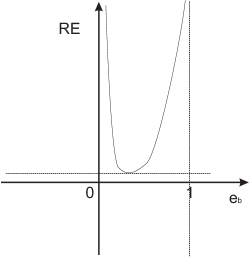
Figure 3.7: Relative Error RE vs discretization coefficient $e_{b}$

So, a bounded discretization error $\delta\tilde{\textbf{E}}$ is essential for an accurate solution to balance the solution approximation error and the ill conditioning of the linear system.

3.5 Summary

The proposed method intends to approximate a vector field from a set of line integrals. As we showed, from $4N$ boundary measurements, the maximum number of equations which can be obtained taking all possible pairs of boundary measurements is $2N(4N-1)$ and the maximum number of independent line integrals cannot exceed the $4N-1$ equations. In the case of a square domain with $2N^{2}$ unknowns, this number of independent continuous line integrals is not sufficient for the recovery of a $2D$ irrotational vector field. However, we provided a theoretical proof showing that the discretization can be an efficient way of regularizing the continuous ill posed problem and therefore the problem is tractable by solving it in the discrete domain.

Chapter 4 Simulations and a Real Application

The current chapter is divided into two main parts: in the first part the validation and verification of the line integral method is presented performing some basic simulations while in the second part an introduction to the inverse bioelectric field problem is reported as a future real application of the proposed vector field reconstruction method.

In particular, for the evaluation of the method we perform simulations for the approximately reconstruction of an electrostatic field produced by electric monopoles in a $2D$ square domain based on the vector field recovery method. According to the preconditions and assumptions of the mathematical model, the electrostatic field is a good example for the validation of the method as it satisfies the quasi static condition and the irrotational property.

Moreover, the numerical implementation of the method is based on the modeling described in subsection 3.2.3 where nearest neighbor approximation was employed. For the verification of the theoretical predictions, the magnitude of the singular values of transfer matrix A of system 3.5, will provide a measure of the invertibility and conditioning of the numerical system 3.5. The sampling step along the line integrals will be very small (much smaller than the cell size) in all simulations.

Finally, the proposed vector field method will be presented as an equivalent mathematical counterpart of the partial differential formulation of the inverse bioelectric field problem [17]. Comparisons of the two approaches will be made.

4.1 Results

The qualitative and quantitative evaluation of the method is very important for examination of its robustness. The validation is concerned with how the mathematical and geometric formulations represent the real physical problem and the verification assesses the accuracy with which the numerical model approximates the real one. The mathematical and geometric properties of the experimental model are defined in the “Simulation Setup” subsection while in subsection “Simulations using Electric Monopoles” the evaluation of the previous theoretical findings is performed.

4.1.1 Simulation Setup

Geometrical Model

In the current simulations we intend to recover a vector field in a $2D$ square bounded domain $\Omega$. For the numerical estimation of the field, the discretization of $\Omega$ is essential. Discretization of the domain can be described as

$$\Omega:\{(x,y)\in[-U,U]^{2}\}\underbrace{\rightarrow}_{Discretization}\{[i,j]\in[1:N,1:N]\}$$

where $i=\left\lfloor\frac{x+U}{P}\right\rfloor$, $j=\left\lfloor\frac{y+U}{P}\right\rfloor$ (nearest neighbor approximation) with $[P\times P]$ the cell’s size and $N=2U/P$ the spatial resolution (sampling rate) of the discrete domain.

Mathematical Model

The numerical representation of the line integral equations is given by

$$\tilde{I}_{L_{\rho,\phi}}=\sum N_{ij}\textbf{E}[i,j]\cdot(\cos\phi,\sin\phi)\Delta r$$ (4.1)

where $N_{ij}$ is the number of samples in cell $[i,j]$ of the domain and $\Delta r$ the sampling step. The linear system of equations is designed according to subsection 3.2.2.

Source Model

A set of monopoles is employed for the production of the real electric field. The field created by monopoles (point sources) is given by $\textbf{E}=k\sum_{i}\frac{Q_{i}}{(r-r_{i})^{2}}\hat{\textbf{r}}_{i}$ where $(r-r_{i})^{2}$ is the distance between charge $Q_{i}$ and the E-field evaluation point r and $\hat{\textbf{r}}_{i}$ the unit vector pointing from the particle with charge $Q_{i}$ to the E-field point. $\Phi=k\sum_{i}\frac{Q_{i}}{|r-r_{i}|}$ is the potential function for the estimation of the potential values at the boundaries of the domain.

So, in the inverse vector field problem, one seeks to estimate field $\textbf{E}[i,j]$ in each cell $[i,j]$ when the potential values in the middle of the boundary edges of the boundary cells are known.

The linear system 3.5 is formulated from a set of approximated line integrals (4.1), where value $\tilde{I}_{L_{\rho,\phi}}$ is the potential difference between two boundary points.

In most simulations, the point sources of the field were positioned outside the bounded domain in order to avoid singularities, since in practical problems the value of the field cannot be infinite.

In the next subsection we examine the following scenarios:

• increase the resolution of the interior of the discrete domain and the observed boundary measurements and examine the relationship between the resolution and the ill conditioning of the system 3.5;

• create a field using more point sources with arbitrary charges and positions but still outside the bounded domain for constant resolution;

• place the point source inside the domain.

The goal is to examine experimentally the ill conditioning of the system for different source distributions (close and far from the bounded domain) and the relationship between the spatial resolution of the domain and the ill conditioning. For the examination of the ill conditioning, the singular values of transfer matrix A of the linear system 3.5 are estimated performing the singular value decomposition (SVD) of A. It is known that a slowly decreasing singular value spectrum with a broader range of nonzero singular values indicates a better conditioning while a rapidly decreasing to zero shows increase of ill conditioning. Moreover, a second indicator is the condition number $k(\textbf{A})=\frac{\sigma_{max}}{\sigma_{min}}$ where $\sigma_{max}$ and $\sigma_{min}$ are the maximum and minimum singular values of A, respectively. The condition number is a gauge of the transfer error from matrix A and vector b (eq. 3.5) to the solution vector x. When the condition number is close to 1, the conditioning of the system is good and the transfer error is low. So, small changes in A or b produce small errors in x. Finally, we estimate the relative error of the magnitude and the phase between the approximated and the real field using

$$RE=\frac{\|\textbf{x}_{LS}-\textbf{x}_{exact}\|_{2}}{\|\textbf{x}_{exact}\|_{2}}$$ (4.2)

where $\|\textbf{x}\|_{2}=\sqrt{\sum_{i}x_{i}^{2}}$.

4.1.2 Simulations using Electric Monopoles

• In the first set of simulations the sources are selected to be far from the recovery domain in order the field to be smooth and thus to examine only the relationship between resolution and ill conditioning due to grid refinement.

  $1^{st}Example\\$

  For a bounded domain $\Omega:\{(x,y)\,\,\in\,\,[-U,U]^{2}\subset\Re^{2}\}=[-5.5,5.5]^{2}$ and two point sources with the same charge $Q$ placed at $(-19,0)$ and $(19,19)$ on the $x,y$ coordinate system (far from the domain $\Omega$) and small sampling step $\Delta r=10^{-4}U$ along the integral line, we obtain the following.

  When $P\times P=1\times 1$, the cell size and grid is $11\times 11$ (resolution is 11), the recovered field is depicted in figure 4.1B.

  

  Figure 4.1: (A) Real Field and (B) Recovered Field when the grid resolution is $N=2U/P=11.$

  The condition number of the transfer matrix A of the linear system is $k(\textbf{A})=174$ and the relative errors (eq. 4.2) of the magnitude and the phase between the real and the reconstructed field are $RE_{magnitude}=0.11$ and $RE_{phase}=0.05$ respectively.

  

  Figure 4.2: Refining the grid resolution, (A) Real Field and (B) Recovered Field when the grid resolution is $N=2U/P=22$.

  When the cell size is $P=0.5$, the condition number is $k(\textbf{A})=10^{4}$ and the relative errors $RE_{magnitude}=0.08$ and $RE_{phase}=0.045$. The recovered field is showed in figure 4.2B. In both cases $\Delta r$ is much less than the cell size $P$. As we can observe the condition number in the second case in much higher than in the first case where the spatial resolution is “coarse”. This implies that the solution of the second system $\textbf{A}\textbf{x}_{LS}=\textbf{b}$ is more sensitive and unstable to A or b perturbations.

  System instability means that the continuous dependence of the solution upon the input data cannot be guaranteed and in the presence of input noise (perturbations) the system behavior is unpredictable. In the current simulations there is no additional noise or other external sources of error, so the ill conditioning of the system (intrinsic ill conditioning) due to the high condition number $k(\textbf{A})$ of order $10^{k}$ has an effect on the computed solution in the sense that a loss of $k$ digit accuracy in the solution is applied (rule of thumb [24]). Thus, for a floating point arithmetic (16 digits floating point numbers are used generally in these simulations) only $16-k$ digit solution accuracy can be achieved. So, in the absence of sources of noise, there is mainly a loss in accuracy when the condition number is high while there no great effect on the system’s stability.

  The approximation error RE is lower for the “refined” system (Res. 22) than that of the “coarse” system (Res. 11). In the “refined” system, there is a loss of $4$ digits in the solution accuracy which is not so high for floating point measurements and due to grid refinement, more spatial frequencies of the field can be recovered. Thus, the solution of the “refined” system is more accurate. However, the “refined” system is more unstable and if the spatial resolution of the problem tends to the continuous case then obviously the linear system will tend to rank deficiency.

  

  Figure 4.3: Refining the grid resolution, the spectrum of the singular values (dotted line) descents more rapidly to zero.

  Moreover, grid refinement results the faster descent of the singular values of the spectrum to zero and frequently a narrower range of non zero singular values, which also indicate that the conditioning of the transfer matrix A and the stability of the linear system deteriorates. This is clear according to figure 4.3 where the continuous line depicts the singular values spectrum when the grid resolution is $N=U/P=11$ and the dashed line the spectrum for $N=22$.

  $2^{nd}Example\\$

  Further results for $2$ point sources with $Q=10^{-8}$ localized again at $(-19,0)$ and $(19,19)$ (far away from the bounded domain $\Omega:\{(x,y)\in[-2.5,2.5]^{2}\}$) and 3 different cell sizes $P=1,0.5,0.25$ are presented in table 4.1 and figure 4.4.

  

  Figure 4.4: When refining the grid resolution, the spectrum of the singular values descents more rapidly to zero and thus the conditioning of the system deteriorates. In this example, 2 point sources with $Q=10^{-8}$ localized at $(-19,0)$ and $(19,19)$ (far away from the bounded domain $\Omega:\{(x,y)\in[-2.5,2.5]^{2}\}$) and 3 different cell sizes were used $P=1,0.5,0.25$.

  Resolution	Cell Size	Measurements
  $N\times N$	P	k(A)	$RE_{Magnitude}$	$RE_{Phase}$
  $20\times 20$	$0.25$	$219.2$	0.0168	0.0048
  $10\times 10$	$0.5$	$93.16$	0.024	0.008
  $5\times 5$	$1$	$96.7$	0.044	0.013

  Table 4.1: Condition number $k(\textbf{A}$) and relative errors for different resolution levels

• When a large number of point sources (160 sources with arbitrary charges) are placed far from domain $\Omega$ (fig.4.6) then $RE_{magnitude}=0.1567$ $RE_{phase}=0.1527$ and the recovered field is depicted in figure 4.5.

  

  Figure 4.5: (A) Real Field and (B) Recovered Field when the grid resolution is $N=2U/P=11$ and the real field is produced from many point sources which are around the vector field domain.

  

  Figure 4.6: Dots depict the locations of the point sources far from the bounded domain and the arrows the recovered vector field inside the bounded domain

  If the point sources are closer to the field of interest, like in figures 4.7 and 4.8, and keeping constant resolution, the relative errors are $RE_{magnitude}=0.63$ and $RE_{phase}=0.33$. Clearly, the relative errors increase as the field sources are placed closer to the recovery domain.

  

  Figure 4.7: (A) Real Field and (B) Recovered Field when the grid resolution is $N=2U/P=11$ and the sources are closer to the bounded domain

  

  Figure 4.8: Dots depict the locations of the point sources which are closer to the bounded domain and the arrows depict the recovered vector field inside the bounded domain

  

  Figure 4.9: Recovered field when two point sources are inside the bounded domain

• In the case where the sources are localized inside the bounded domain, the relative error of the magnitude of the field is too high while the phase error is low and the vector arrows point to the sources’ positions. The field close to sources is not smooth, i.e. the real field has both high and low spatial frequency terms and thus for poor spatial resolution of the bounded domain (fig. 5.1): only the low spatial frequency terms can be recovered. The same actually happens in the previous case (fig.4.8) when the point sources are placed closer to the grid. In figure 5.1 the relative error of the magnitude is high due to low resolution. However, the recovered field points at the source locations which indicates that the low spatial frequency terms give some extremely useful information about the direction of the field.

Condition number vs Resolution

Finally, figure 4.10 depicts the grid resolution against the condition number of the transfer matrix of the linear system. By construction the transfer matrix of the linear system depends on the geometrical characteristics of the region where we intend to estimate the field and the change of the resolution. So, as our experiments are performed in a rectangular region then for constant resolution all the examples share the same transfer matrix and what it changes in our linear system basically is the boundary measurements b. Therefore, the following graph presents the relationship between the rectangular resolution and the conditioning of the transfer matrix.

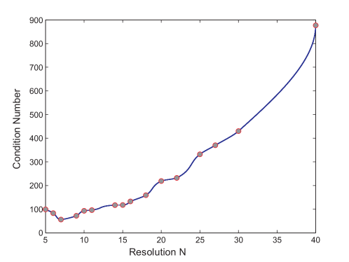
Figure 4.10: Condition number for increasing values of grid resolution $N\times N$.

So, one more time we conclude that different discretization choices of the grid impact the formulation of matrix A and the increase in spatial resolution actually increases the ill-conditioning of this inverse problem.

The effect of additive noise on the reconstruction

In this paragraph we examine the effect of noise in b measurements of the linear system $\textbf{A}\textbf{x}_{LS}=\textbf{b}$ for the $2^{nd}example$ of the previous subsection where the field was produced by $2$ point sources with $Q=10^{-8}$ localized at $(-19,0)$ and $(19,19)$ far from the bounded domain $\Omega:\{(x,y)\in[-2.5,2.5]^{2}\}$. According to figure 4.10 the lower acceptable value of condition number $K(\textbf{A})$ is $72$ such as to balance ill conditioning-resolution $N\times N=9\times 9$. So the majority of the rest simulations with noisy measurements will be performed for this resolution however, some further simulations with higher condition number will be estimated in order to examine the stability of the system in the presence of noise. Moreover, we employ the relative magnitude of the input and output error to provide a measure of stability factor $S$:

$$e_{out}=\frac{\|\textbf{x}_{LS}-\textbf{x}_{exact}\|_{2}}{\|x_{exact}\|_{2}}$$

$$e_{in}=\frac{\|\bar{\textbf{b}}-\textbf{b}\|_{2}}{\|\textbf{b}\|_{2}}$$

$$S=\frac{e_{out}}{e_{in}}$$

Noisy measurements are estimated according to $\bar{\textbf{b}}=\textbf{b}+n\cdot randn()$ where $randn()$ is Matlab function which produce random numbers whose elements are normally distributed with mean $0$, variance $\sigma^{2}=1$ and $n\in[5\cdot 10^{-3},5\cdot 10^{-2}]$ In figure 4.11 for each $n$ value, we estimate the mean value of $e_{out}$ using $100$ different noise vectors. Stability factor was estimated between $8.5\sim 9.5$ (we have to mention that $S$ is meaningless for $\bar{\textbf{b}\rightarrow\textbf{b}}$.)Particulary, x-axis depicts the Signal to Noise ratios (SNR)of our inputs which are given by $20log_{10}(1/mean(e_{i}n)_{n})$ while y-axis the mean values of $mean(e_{out})_{n}$. Obviously for higher values of the SNR (low additive noise) the output relative error is low.

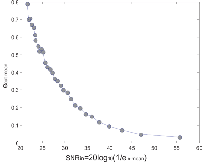
Figure 4.11: Mean values of the output error $e_{out}$ for different values of the input SNR when the condition number of the transfer matrix is low.

For the case where the condition number is a bit higher i.e. $\textbf{A}=132.6$ and $N\times N=16\times 16$ the curve between $e_{out}$ and SNR is depicted in figure 4.12.

Figure 4.12: Mean values of the output error $e_{out}$ for different values of the input SNR and $S$ factor range between $14.1\sim 18$.

Comparing figures 4.11 and 4.12 and stability factors $S$ we can mention that the increase in the ill conditioning of the problems(even a small increase) affects the accuracy of the output solution in the presence of noise. Obviously when the level of noise is high and we need a better accuracy(grid refinement) then extra regularization such as Tikhonov should be considered and possible pre-processing of the measurements to reduce noise level.

4.1.3 Discussion

Different discretization choices of the grid will impact the formulation of matrix A. The increase in discretization resolution on the bounded domain $\Omega$ actually increases the ill-conditioned nature of the inverse problem. The ill conditioning of the linear system results in the instability of the solution of the system especially in the presence of noise. In the current simulation, there was no additional noise. However, the majority of real problems suffer from additive or multiplicative noise and a future examination of the effect of noise to the inverse problem will be performed.

In order to alleviate the ill conditioning of the linear system, one may perform a coarse discretization of the bounded domain. This leads to a “rough” approximation of the vector field (see fig. 4.8). For a non-smooth field (fig.5.1) the approximation error is considerable. Particularly, let us consider vector field $\textbf{E}(x,y)$ in bounded domain $\Omega$ as the sum of spatial frequency terms according to Fourier series expansion

$$\textbf{E}(x,y)=\sum_{\textbf{k}}\textbf{e}_{k}e^{i\textbf{k}\langle x,y\rangle}+\bar{\textbf{e}}_{k}e^{-i\textbf{k}\langle x,y\rangle}$$

The spatial frequency k is directly related to the spatial resolution of the domain and basically the resolution determines the spatial frequency band limit of the vector field to be recovered. If the resolution of the domain is high then more spatial frequency terms can be recovered. However, the “uncontrolled” increase in resolution worsens the problem conditioning. So, the mathematical and experimental choice of the optimal discretization of the bounded domain, such as to minimize the approximation error while maximizing the stability of the linear system needs to be assessed.

4.2 Practical Aspects Of The Method

A major objective of this section is to introduce the inverse bioelectric problem as one of the most prominent biomedical potential applications of the proposed vector field method. Moreover, a comparison of the line integral method with the current partial differential formulation will be presented.

4.2.1 Inverse Bioelectric Field Problem

The bioelectric field [23] is the manifestation of the current densities inside the human body as a result of the conversion of the energy from chemical to electric form (excitation) in the living nerves, muscles cells and tissues in general.

Bioelectric inverse techniques intend to estimate the source distributions inside specific parts of the body, e.g brain and heart, employing the EEG or ECG recordings (passive methods). The ordinary mathematical modeling of this problem is based on the solution of a boundary value problem of an elliptic partial differential equation (PDE). As we will see later, this problem is ill-posed as it does not satisfy some of the three Hadamard’s criteria: existence, uniqueness of the solution and continuous dependence of the solution upon the data.

4.2.2 PDE Methods

The bioelectric field problem can be formulated in terms of either the Poisson or the Laplace equation depending on the physical properties of the problem [3].

In particular, for the problem formulation, physical characteristics of the electrical sources of the human body have to be defined [23]. The primary source $\rho(x,y)$ of electric activity is produced as a result of the transformation of the energy inside the cells from chemical to electric, which consequently induces an electric current of the form $\sigma\textbf{E}$, where $\sigma$ is the bulk conductivity of the volume. In general, the electric density is time-varying, however, the passive way of the data acquisition (not imposed external potentials like in electrical impedance tomography) using EEG or ECG to record bioelectric source behavior in low frequencies (frequencies below several kHz) [17],[7] enables the quasi-static treatment of the problem. The static consideration of the field in a negligible short time implies that the capacitance component of the tissues ($j\omega\textbf{E}$) can be assumed negligible.

So, the total current density is given by $\textbf{J}=\rho(x,y,z)+\sigma\textbf{E}$ and due to the quasi-static condition it obeys $\nabla\cdot\textbf{J}=0$. A last important point is that electromagnetic wave effects are also neglected [7] and therefore the electric field is given by $\textbf{E}=-\nabla\Phi$.

Poisson Equation Formulation

The commonly used inverse bioelectric methods try to calculate the internal current sources J given a subset of electrostatic potentials measured on the scalp or other part of the body, the geometry and electrical conductivity properties within this human part.

The physical and mathematical model of the inverse bioelectric problem is derived from $\nabla\cdot\textbf{J}=0$ and the scalar potential representation of the field $\textbf{E}=-\nabla{\Phi}$ in a bounded domain $\Omega$. Hence, the inverse problem is based on the solution of a Poisson-like equation:

$$\nabla\sigma\nabla\Phi=-\rho\,\,\,\,\mbox{in}\,\,\Omega$$ (4.3)

with the Cauchy boundary conditions:

$$\Phi=\Phi_{0}\,\,\,\mbox{on}\,\,\Sigma\subseteqq\Gamma_{T}\,\,\,\,\,\,\,\mbox{and}\,\,\,\,\,\,\,\sigma\nabla\Phi\hat{\textbf{n}}=0\,\,\,\mbox{on}\,\,\Gamma_{T}=\partial\Omega\,$$

where $\Phi$ is the electrostatic potential, $\sigma$ is the conductivity tensor, $\rho$ are the current sources per unit volume, and $\Gamma_{T}$ and $\Omega$ represent the surface and the volume of the body part (e.g. head), respectively.

The Dirichlet condition ($\Phi=\Phi_{0}\,\,\,\mbox{on}\,\,\Sigma\subseteqq\Gamma_{T}$) is a mathematical abstraction of potential measurements on $\Sigma$, which are in reality obtained from only a finite number of electrodes, and the Neumann condition ($\sigma\nabla\Phi\hat{\textbf{n}}=0\,\,\,\mbox{on}\,\,\Gamma_{T}=\partial\Omega$) is describing that no current flows out of the body.

For the solution of the problem, the modeling of the sources is extremely essential and the difficulties of the design of an accurate model impose significant limitations to the current solution techniques.

In particular, usually the sources are mathematically assumed to be dipoles with unknown magnitude, position, and orientation [17],[3]. The simplest problem uses the assumption that $\rho=Q(m,P,O)$ is a single dipole, characterized by three parameters (six degrees of freedom), corresponding to magnitude $m$, position $P(x,y,z)$, and orientation $O$. These parameters are adjusted such that the resulting electrostatic potential best matches the given measured data (trial and error method)[17]. More general models with several dipoles and consequently increased number of unknown parameters have been designed. Unfortunately, more general cases where there are no previous assumptions about the sources have no unique solution. Solutions can only be found with suitable regularization or a restriction of the solution space by assuming $\rho$ of a special form.

Generally, the inverse bioelectric field problem (4.3) is ill posed as for an arbitrary source distribution, it does not have a unique solution and the solution does not depend continuously on the data i.e. small errors in measurements may cause large errors in the solution.

More specifically, according to Helmholtz’s theorem earlier, and Thevenin’s (Norton’s) theorem later [18],[23], it is always possible to replace a combination of sources and associated circuity with a single equivalent source and a series of impedances. Thus, circuits with different structure (impedances’ sequence and source location) can give the same equivalent circuit (Thevenin circuit). Similarly, in the electric field which can be assumed as an equivalent representation of a circuit, a different source distribution can give the same equivalent source-generator (Superposition Principle) which gives rise to the observed weighted boundary potentials. In other words, the same observed potential measurements could be produced from different source distributions and thus the problem has not unique solution. So, for the estimation of the sources the common method [23] is to breaks up the solution domain into a finite number of subdomains. In each subdomain, a simplified model of the actual bioelectric source (such as a dipole) is assumed. The problem then is to find the magnitude and direction of each of the simplified sources in the subdomains.

In addition, theoretically the elliptic equations boundary value problem of Poisson PDE with Cauchy boundary conditions leads to an over-specified or too “sensitive” boundary value problem [25] resulting large errors in the solution for small changes in boundary conditions. So, regularization techniques should be performed for the stability of the solution [34].

Laplace Equation Formulation

If the inverse problem is formulated such as there are no sources on the bounded domain, then we obtain the homogeneous counterpart of the Poisson equation. These are the cases where there is interest on the estimation of the potential distribution on a surface (e.g. cortex or surface of the heart) and not in the whole volume from boundary measurements (like scalp (EEG) or torso (ECG) recordings) and hence the sources are out of the region of interest.

So, the Cauchy boundary value problem is formed by Laplacian equation $\nabla\sigma\nabla\Phi=0$. This is also an ill posed problem in the sense that the solution does not depend continuously on the data. Numerically, the solution of the Laplace’s equation can be formulated as $\textbf{A}\Phi=\Phi_{boundaries}$. As the continuous problem is ill posed due to its physical nature [34],[25], matrix A will be ill conditioned.

There are different regularization methods and numerical techniques for the approximate solution of this system [16],[34]. In the current section, we will not give further details about these techniques. However, a brief comparison between Laplace’s equation and the line integrals methods for the estimation of a vector field will be presented.

4.2.3 Vector Field Method

In the previous description, the inverse bioelectric theory intends to estimate the positions and strengths of the sources within a volume (e.g brain) that could have given rise to the observed potential recordings under the assumptions that the field is quasi-static and irrotational. Obviously, the physical principles of the bioelectric field are fitted well with the preconditions and assumptions of the proposed vector field tomographic method. Thus, the proposed method can be applied to recover a bioelectric field in discrete points using the boundary information without needing any prior information about the sources’ formulation while the boundary conditions are automatically satisfied as they are directly incorporated in the line integral formulation.

Vector Field Recovery with Laplace and Vector Field Method

We present the recovery of vector field in a bounded domain $[-5.5,5.5]^{2}$ with cell size $P\times P=1\times 1$, grid $N\times N=11\times 11$ and sampling step $\Delta r=0.0001P$, solving two systems of linear equations where one was derived from the line integral method as it was described previously and another from the numerical solution of the Laplace equation

$$\nabla^{2}\Phi=\frac{\partial^{2}\phi}{\partial x^{2}}+\frac{\partial^{2}\phi}{\partial y^{2}}=0$$

based on the finite difference approximation

$$\frac{\partial^{2}\phi}{\partial x^{2}}=\frac{\phi_{i+1,j}-2\phi_{i,j}+\phi_{i-1,j}}{h^{2}}\,\,\,\frac{\partial^{2}\phi}{\partial y^{2}}=\frac{\phi_{i,j+1}-2\phi_{i,j}+\phi_{i,j-1}}{h^{2}}$$

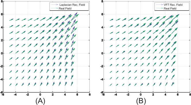
Figure 4.13: The recovered fields applying (A) numerical solution of a Laplacian equation and (B) vector field line integrals, produced by a point source $Q=10^{-8}$ localized in $(13,15)$.

For the recovery of the field in figure 4.13A, the rows of system $\textbf{A}\Phi=\Phi_{boundaries}$ were defined according to

$$4\phi_{i,j}-\phi_{i-1,j}-\phi_{i+i,j}-\phi_{i,j-1}-\phi_{i,j+1}=0$$

with known boundary potential values $\phi_{0,j},\phi_{i,0},\phi_{0,N}$ and $\phi_{N,j}$. After the estimation of $\phi$ the vector field was calculated by

$$\textbf{E}=\left(\frac{\phi_{i+1,j}-\phi_{i-1,j}}{h},\frac{\phi_{i,j+1}-\phi_{i,j-1}}{h}\right)$$

with $h=P$. The coarse recovery of an electrostatic field employing the vector field method presented better and more accurate results than the finite difference Laplacian solution. Here, we have to consider that E is estimated from the potential values $\Phi$ and thus extra numerical errors were introduce to the Laplacian solution.

Chapter 5 Conclusions

Over the past two decades there has been an increasing interest in vector field tomographic methods and many mathematical approaches based on ray and Radon Transform theory have been reported. Nowadays, there is a lack of potential applications, although all the theoretical findings and the previous work may be extremely essential for the evolution and the implementation of robust techniques. Particulary, the theoretical and experimental study of the proposed vector field method for real problems with simple physical and geometric properties is the first step towards the deeper understanding and the evolution of the method for more complex real applications. Briefly, our future work will be focused on three basic tasks:

• robust theoretical formulation of the vector field method according to inverse problems theory;

• more sophisticated numerical approaches based on finite elements theory and further experiments and simulations;

• practical aspects of the method especially in the field of inverse bioelectric field problem with comparisons between the vector field method and the current PDE methods.

5.1 Future Work

• Theoretical Foundation
  In subsection 3.3, basic physics principles are used to describe the ill conditioning of the vector field method and a more intuitive consideration of the ill posedness of the problem was given. Next step is the robust mathematical formulation of this inverse problem in Hadamard’s sense, examining the uniqueness of the solution and the stability of the solution to the noise in the input data.

  In the mathematical theory of the inverse problems, an inverse problem is described by the equation

  $$K\textbf{x}=y$$

  where given $y$ and $K$ we have to solve for x.

  The vector field method is an inverse problem where operator $K$ is an integral operator. This integral operator is compact in many natural topologies and in general it is not one-to-one [20]. Almost always compact operators $K$ are ill posed. However, this basic knowledge is not enough for the mathematical interpretation of the ill posedness of the vector field problem, so further theorems of the inverse problem theory, and assumptions should be considered. A robust and complete mathematical formulation of the problem is essential for a better understanding of the problem’s nature and the potential numerical adaptations of this theoretical problem to real applications.

• Numerical Implementation and Further Experiments
  The numerical solution of the vector field recovery method is based on the discretization of the problem. Ill posedness of the continuous problem is expressed as ill conditioning of the system of linear equations in the discrete version. The conditioning of the problem depends on the resolution of the discrete domain and the applied interpolations schemes. A “naive” discretization may lead to disastrous results as for very “coarse” discretization, the approximation errors increase while when an extreme grid refinement is applied, the conditioning of the numerical system deteriorates.

  In particular, the grid refinement can be used to increase the resolution in bounded domains, but must be used with care because refined meshes worsen the conditioning of the inverse problem and simultaneously increase the computational cost. So, there is an open question about the optimal discretization of the bounded domain, such as to minimize the approximation error while maximizing the stability of the linear system. For this purpose, discretization error bounds should be estimated mathematically and experimentally. Moreover, the discretization of the domain employing other elements, not cells or tiles as in the square domain, embedding more sophisticated techniques should be considered.

  Another option to overcome the ill conditioning of the problem is by increasing the observed data available on the boundary (increase boundary resolution). For the case of a simple $2D$ square domain, there is an initial approach for the definition of the optimum number and positions of the boundary measurements reported in [9]. However, further investigation and generalization for arbitrary shapes of the bounded domain need to be considered. Moreover, it should be mentioned that the increase of boundary measurements is not a very efficient way to solve the problem as in practical applications (e.g. EEG) there are only a few measurements and from these few measurements we have to extract as much information as possible. Finally, the increased boundary resolution, not as a consequence of the increasing measured data but as a results of interpolation schemes [34], does not improve the problem conditioning in real problems.

  

  Figure 5.1: Recovery of the field using the vector field method for an arbitrary boundary shape.

• After the theoretical and the numerical schemes have been completed, the next steps are the EEG application.
  In ordinary EEG source analysis, the inverse problem estimates the positions and strengths of the sources within the brain that could have given rise to the observed scalp potential recordings. In the current project, the final stage is the implementation of a different approach for the EEG analysis employing the proposed method. Rather than performing strengths estimation or location of the sources inside the brain, which are very complicated tasks, a reconstruction of the corresponding static bioelectric field will be performed based on the line integral measurements. This bioelectric field can be treated as an “effective” equivalent state of the brain. Thus for instance, health conditions or a specific pathology (e.g. seizure disorder) may be recognized. This can be achieved by designing a slice-by-slice reconstruction algorithm for vector field recovery or the $3D$ extension of the proposed theoretical model where new numerical problems concerning the design of huge linear systems (sparse matrices and different computational strategies) arise.

Appendix A Rank of Perturbed Matrix $\bar{\textbf{A}}$

As it is described in [24] $p.216$, the rank of a perturbed matrix $\bar{\textbf{A}}=\textbf{A}-\textbf{E}$ is equal to or greater than the $rank(\textbf{A})$ when the entries of E have small magnitude. According to the proof on $p.217$ [24] matrix A with $Rank(\textbf{A})=p$ can be transformed in an equivalent matrix (rank normal form) when elementary row and column operators are applied i.e.

$$\textbf{A}\sim\left(\begin{array}[]{cc}\textbf{I}_{p}&\textbf{0}\\ \textbf{0}&\textbf{0}\end{array}\right)$$

Equivalently for the $\textbf{A}-\textbf{E}$ where $\textbf{E}=\left(\begin{array}[]{cc}\textbf{E}_{11}^{p\times p}&\textbf{E}_{12}\\ \textbf{E}_{21}&\textbf{E}_{22}\end{array}\right)$ we obtain

$$\textbf{A}-\textbf{E}\sim\left(\begin{array}[]{cc}\textbf{I}_{p}-\textbf{E}_{11}^{p\times p}&\textbf{0}\\ \textbf{0}&\textbf{S}\end{array}\right)$$

Thus,

$$\begin{split}Rank(\textbf{A}-\textbf{E})&=Rank(\textbf{I}_{p}-\textbf{E}_{11}^{p\times p})+Rank(\textbf{S})=\\ &=Rank(\textbf{A})+Rank(\textbf{S})\geqslant Rank(\textbf{A})\end{split}$$

In practical problem, $\textbf{S}=\textbf{0}$ is very unlikely as the perturbation (discretization or roundoff errors) is almost “random”. Therefore $Rank(\textbf{A}-\textbf{E})>Rank(\textbf{A})$.

Bibliography

- [1] G. B. Arfken and H. J. Weber. Mathematical Methods for Physicists. Elsevier Academic Press, 6th edition, 2005.
- [2] H. Braun and A. Hauck. Tomographic reconstruction of vector fields. Signal Processing, IEEE Transactions on, 39(2):464 –471, 1991.
- [3] J. D. Bronzino, editor. Biomedical Engineering Fundamentals. Richard C. Dorf-University of California, Davis. Joseph D. Bronzino, 3rd edition, 2006.
- [4] M. Defrise and G. T. Gullberg. 3D reconstruction of tensors and vector. Technical report, Lawrence Berkeley National Laboratory, 2005.
- [5] R. Diestel. Graph Theory. Springer Verlag New York-Electronic Edition 2000, 1997.
- [6] N. Duric, P. Littrup, L. Poulo, A. Babkin, R. Pevzner, E. Holsapple, O. Rama, and C. Glide. Detection of breast cancer with ultrasound tomography: first results with the computed ultrasound risk evaluation (cure) prototype. Med. Physics, 34(2):773–85, Feb. 2007.
- [7] D. B. Geselowitz. On bioelectric potentials in an inhomogeneous volume conductor. Biophysical Journal, 7(1):1–1, 1967.
- [8] A. Giannakidis, L. Kotoulas, and M. Petrou. Virtual sensors for 2d vector field tomography. J. Opt. Soc. Am. A, 27(6):1331–1341, 2010.
- [9] A. Giannakidis and M. Petrou. Sampling bounds for 2d vector field tomography. J. Math. Imaging Vis., 37(2):151–165, 2010.
- [10] S. Helgason. The Radon transform(Progress in Mathematics), volume 5. Birkhauser, 2nd edition, 1999.
- [11] H. M. Hertz. Kerr effect tomography for nonintrusive spatially resolved measurements of asymmetric electric field distributions. Appl. Opt., 25(6):914–921, 1986.
- [12] Q. Huang, Q. Peng, B. Huang, A. Cheryauka, and G. Gullberg. Attenuated vector tomography: An approach to image flow vector fields with doppler ultrasonic imaging. Technical report, Lawrence Berkeley National Laboratory, 2008.
- [13] T. Jansson, M. Almqvist, K. Strahlen, R. Eriksson, G. Sparr , H. Persson, and K. Lindstr m. Ultrasound doppler vector tomography measurements of directional blood flow. Elsevier-Ultrasound in Medicine & Biology, 23(1):47–57, 1997.
- [14] I. Javanovic. Inverse Problems in Acoustic Tomography: Theory and Applications. PhD thesis, EPFL, 2008.
- [15] Johnson. Measurements and reconstruction of three-dimensional fluid flow. United States Patent, 1979.
- [16] C. R. Johnson. Computational and numerical methods for bioelectric field problems. In Critical Reviews in BioMedical Engineering, pages 162–180. CRC Press, Boca Ratan, 1997.
- [17] C. R. Johnson, R. S. MacLeod, and M. A. Matheson. Computational medicine: Bioelectric field problems. Computer, 26:59–67, 1993.
- [18] D. H. Johnson and I. Introduction. Scanning our past - origins of the equivalent circuit concept: The voltage-source equivalent. 2003.
- [19] S. A. Johnson, J. F. Greenleaf, W.A. Samayoa, F.A. Duck, and J. Sjostrand. Reconstruction of three-dimensional velocity fields and other parameters by acoustic ray tracing. In 1975 Ultrasonics Symposium, pages 46 – 51, 1975.
- [20] A. Kirsch. An introduction to the mathematical theory of inverse problems. Springer-Verlag New York, Inc., New York, NY, USA, 1996.
- [21] M. I. Kramar. A feasibility study about the use of vector tomography for the reconstruction of the coronal magnetic field. PhD thesis, University of Gottingen, 2005.
- [22] L. Lovstakken, S. Bjaerum, D. Martens, and H. Torp. Blood flow imaging - a new real-time, flow imaging technique. IEEE Transactions on Ultrasonics, Ferroelectrics and Frequency Control, 53(2):289–299, 2006.
- [23] J. Malmivuo and R. Plonsey. Bioelectromagnetism : Principles and Applications of Bioelectric and Biomagnetic Fields. Oxford University Press, USA, 1st edition, 1995.
- [24] C. D. Meyer. Matrix Analysis and Applied Linear Algebra. 2000.
- [25] P. M. Morse and H. Feshbach. M Methods of Theoretical Physics. York: McGraw-Hill, 1953.
- [26] S. J. Norton. Tomographic reconstruction of 2-d vector fields: Application to flow imaging. Geophysical Journal International, 97(1):161 – 168, 1988.
- [27] S. J. Norton. Unique tomographic reconstruction of vector fields using boundary data. Image Processing, IEEE Transactions on, 1(3):406 –412, jul 1992.
- [28] N. F. Osman and J. L. Prince. Reconstruction of vector fields in bounded domain vector tomography. In Image Processing, 1997. Proceedings., International Conference on, volume 1, pages 476 –479, 1997.
- [29] L. Otis, D. Pia, C. Gibson, and Q. Zhu. Quantifying labial blood flow using optical doppler tomography. Oral Surgery, Oral Medicine, Oral Pathology, Oral Radiology, and Endodontology, 98(2):189–194, 2004.
- [30] M. Petrou and A. Giannakidis. Full tomographic reconstruction of 2d vector fields using discrete integral data. The Computer Journal, 53(7), 2010.
- [31] J. L. Prince. Tomographic reconstruction of 3d vector fields using inner product probes. IEEE transactions on image processing, 3:216–219, 1994.
- [32] D. Rouseff, K. B. Winters, and T. E. Ewart. Reconstruction of oceanic microstructure by tomography: A numerical feasibility study. J. Geophys. Res., (96:C5):p. 8823–8833, 1991.
- [33] T. Schuster, D. Theis, and A. K. Louis. A reconstruction approach for imaging in 3D cone beam vector field tomography. Journal of Biomedical Imaging, 2008:1–17, 2008.
- [34] D. F. Wang, R. M. Kirby, and C. R. Johnson. Resolution strategies for the finite-element-based solution of the ecg inverse problem. In IEEE Transactions on Biomedical Engineering, volume 57, pages 220–237, 2010.
- [35] P. Wedin. Perturbation theory for pseudo-inverses. BIT Numerical Mathematics, 13:217–232, 1973.
- [36] M. Wei. The perturbation of consistent least squares problems. Linear Algebra and its Applications, 112:231 – 245, 1989.