Squashed toric sigma models and mock modular forms

Abstract

We study a class of two-dimensional $\mathcal{N}=(2,2)$ sigma models called squashed toric sigma models, using their Gauged Linear Sigma Models (GLSM) description. These models are obtained by gauging the global $U(1)$ symmetries of toric GLSMs and introducing a set of corresponding compensator superfields. The geometry of the resulting vacuum manifold is a deformation of the corresponding toric manifold in which the torus fibration maintains a constant size in the interior of the manifold, thus producing a neck-like region. We compute the elliptic genus of these models, using localization, in the case when the unsquashed vacuum manifolds obey the Calabi-Yau condition. The elliptic genera have a non-holomorphic dependence on the modular parameter $\tau$ coming from the continuum produced by the neck. In the simplest case corresponding to squashed $\mathbb{C}/\mathbb{Z}_{2}$ the elliptic genus is a mixed mock Jacobi form which coincides with the elliptic genus of the $\mathcal{N}=(2,2)$ $SL(2,\mathbb{R})/U(1)$ cigar coset.

1 Introduction and summary

The classic work of Schellekens:1986yi ; Witten:1986bf ; Alvarez:1987wg on the elliptic genus led to the establishment of a three-way relation between two-dimensional $\mathcal{N}=(2,2)$ superconformal field theories (SCFTs), compact Calabi-Yau (CY) manifolds, and modular and Jacobi forms. The elliptic genus of an $\mathcal{N}=(2,2)$ SCFT $M$ with central charge $c$ is defined as

$$\chi_{\text{ell}}(M;\tau,z)\;:=\;\mbox{Tr}_{\mathcal{H}_{RR}}\,(-1)^{F}\,q^{L_{0}}\,\overline{q}^{\overline{L}_{0}}\,\zeta^{J_{0}}\,,\qquad q=e^{2\pi i\tau},\quad\zeta=e^{2\pi iz}\,,$$ (1)

where $\mathcal{H}_{RR}$ is the Ramond-Ramond Hilbert space of the theory, $L_{0}$ and ${\overline{L}_{0}}$ are the left and right-moving Hamiltonians of the $(2,2)$ algebra, $J_{0}$ is the left-moving R-charge, and $F$ is the fermion number operator. The elliptic genus of a two-dimensional $(2,2)$ SCFT in the moduli space of a compact CY manifold of complex dimension $d$ is a Jacobi form of weight 0 and index $d/2=c/6$.

In this paper we focus on a class of $\mathcal{N}=(2,2)$ supersymmetric sigma models which flow to SCFTs with non-compact target space. Non-trivial non-compact target spaces appear in diverse physical situations, e.g. as the vacuum manifold of supersymmetric quantum field theories, as supersymmetric black hole moduli spaces, and as backgrounds on which strings and D-branes can propagate (some examples are the near-horizon regions of NS5-branes, ALE spaces, and the conifold). The presence of a continuum of operators in the spectrum, which is a signature of the non-compactness, is a source of many subtleties and often invalidates basic conclusions that apply to theories with compact target space. An example of this phenomenon that we will study in particular in this paper is the holomorphicity of the elliptic genus.

In theories with a discrete spectrum, holomorphicity (in $\tau$) of the elliptic genus follows from the simple argument Witten:1986bf that all states with non-zero $\overline{L}_{0}$ come in representations with equal number of bosonic and fermionic states, and therefore do not contribute to the elliptic genus. When there is a continuum component in the spectrum, the trace in Equation (1) needs a precise definition, and the measure involved in the integral over the continuum may not be equal for bosonic and fermionic states with equal values of $\overline{L}_{0}$. (Physically this means that the density of states of fermions and bosons are not equal, this happens when there is a non-zero phase shift in scattering from infinity.) This can lead to an incomplete cancellation, and therefore to a $\overline{\tau}$-dependence of the elliptic genus.

This phenomenon has been understood in great detail for the supersymmetric version of the Euclidean 2d black hole, also known as the cigar, whose target space is the (Euclidean) $SL_{2}(\mathbb{R})/U(1)$ $\mathcal{N}=(2,2)$ SCFT. The elliptic genus of the cigar theory was calculated in Troost:2010ud ; Eguchi:2010cb ; Ashok:2011cy by computing the relevant functional integral of the WZW coset, using the technique of Gawedzki:1991yu . The same phenomenon was also found, in a spacetime avatar, in string theories in the near-horizon geometry of NS5-branes Harvey:2013mda ; Harvey:2014cva and their T-duals Cheng:2014zpa , all of which involve the cigar SCFT as an important component. The elliptic genus of the cigar coset, as well as some generalizations, was later computed in a much simpler manner using the GLSM description Murthy:2013mya ; Ashok:2013pya . The class of modular objects that captures the modular but non-holomorphic behavior of the elliptic genus of the cigar theory was discovered relatively recently, and is called mock modular forms Zwegers:2002 ; Zagier:2007 (more precisely the cigar elliptic genus is a mixed mock Jacobi form Dabholkar:2012nd ). These functions transform like holomorphic modular forms, but their $\overline{\tau}$-derivative is non-vanishing and can be summarized by a holomorphic anomaly equation (summarized in Appendix A). In this sense the study of the cigar theory has led to an extension of the three-way relation mentioned in the beginning.

While it is nice to see mock modular forms fit into a corner of conformal field theory and string theory, it is worth noting that one of the links in this refinement of the three-way relation has not been well-understood, namely the role of geometry. This paper aims to reduce this gap by studying a class of non-compact manifolds which are thought to flow to SCFTs with a non-trivial dilaton profile, and whose elliptic genus shows interesting new modular behavior. We find functions which depend explicitly on $\overline{\tau}$ but transform like a holomorphic multi-variable Jacobi form. The $\overline{\tau}$-dependence is captured by a differential equation (Equation 93) that generalizes the one obeyed by mock Jacobi forms. We hope that our physical ideas and results serve as a motivation for further work that is needed to understand the links between non-compact manifolds and SCFTs, their elliptic genera, and mock modular forms and their generalizations. These considerations may also be useful for the Umbral Moonshine program Eguchi:2010ej ; Cheng:2012tq ; Cheng:2013wca where one is searching for geometric or physical objects that give rise to particular mock Jacobi forms.

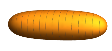
Figure 3: Squashed $\mathbb{C}\mathbb{P}^{1}$ with $\widehat{k}=1/4$ and $r=1$

The objects of study in this paper, called squashed toric manifolds, are deformations of toric manifolds. While toric manifolds have been studied extensively by geometers as well as by string theorists, their squashed counterparts have received less attention. The defining feature of a (real) $2d$-dimensional toric manifold is a non-trivial $U(1)^{d}$ action at a generic point. The geometric structure is that of a $d$-dimensional torus fibered on a $d$-dimensional base. This torus varies in size as we move along the base, and there are distinguished fixed points where the torus shrinks to zero size. The squashing deformation makes the torus gain a constant size in the deep interior of the manifold. A simple illustrative example is that of squashed $\mathbb{C}\mathbb{P}^{1}$ in which the spherical shape gets squashed to a sausage (see Fig 3).

The GLSMs for these squashed toric manifolds were introduced in Hori:2001ax . The starting (unsquashed) point is a model with $n$ chiral superfields and $n-d$ gauge superfields, whose vacuum manifold is $2d$-dimensional. The squashing deformation gauges the $d$-dimensional flavor symmetry of this theory and at the same time introduces a set of $d$ compensator-chiral superfields (which translate under the flavor gauge fields). The vacuum manifold of the squashed model thus remains $2d$-dimensional, and is called the squashed toric manifold. In most of the paper we study manifolds that obey the Calabi-Yau condition, namely the vanishing of the sum of the gauge charges of the chiral multiplets for each gauge field. This condition ensures that the 2d QFTs has non-anomalous chiral $U(1)$ R-symmetries so that they can flow to $\mathcal{N}=(2,2)$ SCFTs. This sum-rule in turn implies that the initial toric manifold (and therefore its squashed deformation) is non-compact Morrison:1994fr . The squashing deformation is a very strong deformation in that it reaches the asymptotic region, for example, if we begin with a space of the form $\mathbb{C}/\mathbb{Z}_{2}$ the squashed counterpart has a cylinder-like shape asymptotically. This is in a different universality class of theories compared to the toric CY manifolds—the Ricci curvature is no longer zero and is supported by a non-trivial dilaton profile. Our main result, that we now describe briefly, is an expression for the elliptic genus of these squashed toric manifolds.

First we recall some results for the elliptic genus of toric CY manifolds. As mentioned above, these manifolds are necessarily non-compact. Although one can formally write down the elliptic genus as in Equation (1) using the $\mathcal{N}=(2,2)$ superconformal algebra, the quantity is usually ill-defined because of the infinite volume of the space. One way to regulate this divergence is to turn on a background Wilson line $u$ of the external gauge field which couples to the angular momentum in the spacetime (which is a flavor charge $F$ in the sigma model). The zero modes of the bosons are charged under this symmetry, and therefore the divergence is lifted. The modified elliptic genus

$$\chi_{\text{ell}}(M_{\text{tor}};\tau,z,u)\;=\;\mbox{Tr}_{\mathcal{H}_{RR}}\,(-1)^{F}\,q^{L_{0}}\,\overline{q}^{\overline{L}_{0}}\,\zeta^{J_{0}}e^{2\pi iuF}$$ (2)

is now a sensible supersymmetric index. This route was used to study the elliptic genus of ALE and ALF spaces in Harvey:2014nha , and the answer thus obtained is a Jacobi form meromorphic in the elliptic variable $u$. This meromorphicity is related to the fact that the scale introduced by the background Wilson line $u$ mildly breaks the infinite-dimensional superconformal algebra, as can be seen from the fact that bosons can no longer be separated into left- and right-moving parts Dabholkar:2010rm ; Haghighat:2015ega .

In this paper we take a different route. The squashing deformation is now an operation intrinsic to the theory and therefore one does not need to introduce any external scale to regulate the elliptic genus. The original definition (1) of the elliptic genus applies to the squashed models as long as we define the trace carefully. The answer turns out to be holomorphic in the elliptic variable $z$, but non-holomorphic in the modular parameter $\tau$.

To be concrete, we consider a $2d$-dimensional toric GLSM $M_{\text{tor}}$, and associate the set of chemical potentials $\{u^{\prime}_{\ell}\}$, $\ell=1,\cdots d$, to the corresponding $U(1)$ symmetries. This GLSM has a flavored elliptic genus $\chi_{\text{ell}}(M_{\text{tor}};\tau,z,\{u^{\prime}_{\ell}\})$ as described above. The $U(1)$ toric symmetries act on the fields of the GLSM as global flavor symmetries with the chiral superfields having charges $F_{i}^{\ell}$, $i=1,\cdots n$. Two sets of parameters that are particularly important for the elliptic genus of the squashed manifold $\widetilde{M}_{\text{tor}}$ are the sum of the charges $b_{\ell}=\sum_{i=1}^{n}F_{i}^{\ell}$ for each flavor symmetry, and the strength of the coupling $\{k_{\ell}\}$ of the compensator fields. We define $\widetilde{k}_{\ell}=k_{\ell}/b_{\ell}^{2}$ which is the effective strength of the squashing deformation, and which determines the size of the constant circles in the squashed manifolds. Our main result is an expression for the elliptic genus of $\widetilde{M}_{\text{tor}}$ given in terms of an integral over the $d$-dimensional torus $E_{\tau}^{d}$, with $E_{\tau}=\mathbb{C}/(\mathbb{Z}\tau+\mathbb{Z})$, spanned by the holonomies $\{u^{\prime}_{\ell}\}$ of the flavor symmetry gauge fields. Define, for $z,u\in\mathbb{C}$, the non-holomorphic kernel function:

$$H_{k}(\tau,z,u)\;=\;k\sum_{m,w\,\in\,\mathbb{Z}}\,e^{2\pi iwz-\frac{\pi k}{\tau_{2}}\bigl{(}w\tau+m+u+\frac{z}{k}\bigr{)}\bigl{(}w\overline{\tau}+m+\overline{u}+\frac{z}{k}\bigr{)}}\,.$$ (3)

The elliptic genus of the squashed toric model $\widetilde{M}_{\text{tor}}$, given in Equation (83) of the text, is a $d$-dimensional convolution of the elliptic genus of $M_{\text{tor}}$ with these kernel functions:

$$\chi_{\text{ell}}(\widetilde{M}_{\text{tor}};\tau,z)\;=\;\bigintsss_{E_{\tau}^{d}}\,\prod_{\ell=1}^{d}\frac{{\mathrm{d}}^{2}u^{\prime}_{\ell}}{\tau_{2}}\,H_{\widetilde{k}_{\ell}}(\tau,z,u^{\prime}_{\ell})\;\chi_{\text{ell}}(M_{\text{tor}};\tau,z,\{u^{\prime}_{\ell}/b_{\ell}\})\,.$$ (4)

This convolution thus shifts the signature of the non-compactness from a meromorphicity in $u$ to a non-holomorphy in $\tau$.

Apart from their intrinsic mathematical interest, these results naturally prompt the conjecture for the existence of an RG flow from the squashed toric sigma models to certain SCFTs with the above elliptic genera. In the simplest example, the RG flow is from a squashed $\mathbb{C}/\mathbb{Z}_{2}$ to the cigar coset SCFT. This RG flow is similar to that discussed in Hori:2001ax but our UV starting point (46) is slightly different. One can make similar conjectures for each of the GLSMs of RG flows from higher-dimensional squashed toric manifolds to SCFTs in the IR. In Gromov:2017 we study, and provide further evidence for, such RG flows.

The plan of the paper is as follows. In Section 2 we review toric manifolds, some of their properties, and their construction as vacuum manifolds of GLSMs. We then review the squashing deformation of Hori:2001ax . In each case we illustrate the discussion with four examples. In Section 3 we present the computation of the elliptic genus of toric CY manifolds using the GLSM construction and the technique of localization. In Section 4 we compute the elliptic genus of the squashed toric models. In Section 5 we analyze a compact (non-Calabi-Yau) example, namely the supersymmetric sausage model, and compute its Witten index. In four appendices we briefly review some details of (multi-variable) Jacobi forms and mock Jacobi forms, the holomorphic construction of toric manifolds, the metric of squashed manifolds, and the action of the GLSMs, that are referred to in various places in the main text.

2 A class of gauged linear sigma models

In this section we review some basic facts about toric manifolds and toric sigma models. This is a wide and deep subject and we refer the reader to Morrison:1994fr ; Hori:2003ic for an introduction to this topic for physicists, and to daSilva:2001 for a mathematical treatment of the symplectic viewpoint on toric manifolds which we follow. Here we shall briefly review the GLSM construction of toric manifolds and present four examples ($\mathbb{C}\mathbb{P}^{1}$, $\mathbb{C}/\mathbb{Z}_{2}$, the $A_{1}$ space $\mathbb{C}^{2}/\mathbb{Z}_{2}$, and the conifold) which we will use in the rest of the paper to illustrate our general results.

2.1 A brief review of toric manifolds and toric sigma models

Consider the $\mathcal{N}=(2,2)$ GLSM with field content consisting of the chiral superfields $\Phi_{i}$, $i=1,\cdots,n$, and the abelian vector superfields $V_{a}$, $a=1,\cdots,n-d$ with associated field strength twisted chiral superfields $\Sigma_{a}$. The chiral superfields have charges $Q^{i}_{a}$ under the vector superfields. The action is:

$$S_{0}\;=\;\frac{1}{2\pi}\int{\mathrm{d}}^{2}x\,\Biggl{[}\int{\mathrm{d}}^{4}\theta\,\biggl{(}\sum_{i=1}^{n}\overline{\Phi}_{i}\,\exp\Bigl{(}\sum_{a=1}^{n-d}Q_{i}^{a}V_{a}\Bigr{)}\Phi_{i}\,-\,{1\over 2e^{2}}\sum_{a=1}^{n-d}\overline{\Sigma}_{a}\,\Sigma_{a}\biggr{)}\,+\,\frac{1}{2}\int{\mathrm{d}}^{2}\widetilde{\theta}\sum_{a=1}^{n-d}t_{a}\Sigma_{a}\,+\,\text{c.c.}\Biggr{]}\,,$$ (5)

with $t_{a}=r_{a}-i\vartheta_{a}$. Here $r_{a}$ is the Fayet-Ilopoulos parameter and $\vartheta_{a}$ is the theta angle for the gauge field $V_{a}$.

The manifold of inequivalent vacua (the vacuum manifold) is obtained by solving the constraints imposed by setting the D-terms^, :

$$D_{a}\;=\;-e_{a}^{2}\,\mu_{a}\,,\qquad\mu_{a}\;=\;\sum_{i=1}^{n}Q_{i}^{a}\,|\phi_{i}|^{2}-r_{a}\,,\qquad a=1,\dots,n-d\,,$$ (6)

to zero, and quotienting by the gauge group $G=U(1)^{n-d}$. Denoting the vector of FI terms with components $r_{a}$ by $r$, we write the $2d$ real-dimensional vacuum manifold $V$ as:

$$V(r)\;=\;\mu^{-1}(0)/G\,.$$ (7)

It is a non-trivial fact that this vacuum manifold has a natural symplectic structure induced from that of $\mathbb{C}^{n}$ on which the chiral fields $\phi_{i}$ live. It inherits a non-trivial $U(1)^{d}$ Hamiltonian action from the $U(1)^{d}$ flavor symmetry of the GLSM (5). Such a manifold $V$ is called a symplectic toric manifold, and the above construction of $V$ is precisely what is called the symplectic quotient construction of toric manifolds daSilva:2001 .

As $\mathbb{C}^{n}$ is also a Kähler manifold and the $U(1)^{n-d}$ action preserves its complex structure, the quotient space $V$ is also a Kähler manifold. The metric can thus be written in terms of local complex coordinates $Z^{I}(\phi_{i})$, $I=1,\cdots d$, as a derivative of the Kähler potential $K(Z_{I},\overline{Z_{I}})$:

$$g_{I\overline{J}}\;=\;\partial_{I}\partial_{\overline{J}}\,K(Z_{I},\overline{Z_{I}})\,.$$ (8)

This will be the case at a generic point in field space for all the models that we discuss in this paper. (The manifolds we discuss typically will also have special points where there are orbifold singularities.) The metric on the quotient space can thus be computed by implementing the quotient construction on $\mathbb{C}^{n}$, or equivalently, by starting with the action (5) and integrating out the gauge fields. We will illustrate both the methods in the following examples.

Example 1: ${\bf\mathbb{CP}^{1}}$, $(n,d)=(2,1)$.

Our first example is $\mathbb{C}\mathbb{P}^{1}$ which can be modelled by one vector superfield and two chiral superfields both with gauge charges $+1$. The two-dimensional vacuum manifold is

$$V(r)\;=\;\{|\phi_{1}|^{2}+|\phi_{2}|^{2}-r=0\}/U(1)\,.$$ (9)

In order to implement the symplectic quotient construction, we write $\phi^{i}=\rho_{i}e^{i\theta_{i}}$ with the radial variables $\rho_{i}\geq 0$ and the angular variables $\theta_{i}\in[0,2\pi]$. The symplectic form on the original $\mathbb{C}^{2}$ is:

$$\omega\;=\;\sum_{i=1}^{2}\,\rho_{i}\,d\rho_{i}\wedge d\theta_{i}\,.$$ (10)

The $D$-term constraint $\rho_{1}^{2}+\rho_{2}^{2}=r$ implies $\rho_{1}d\rho_{1}+\rho_{2}d\rho_{2}=0$. The induced symplectic form is given by

$$\omega\;=\;\rho_{1}\,d\rho_{1}\wedge d(\theta_{1}-\theta_{2})\,.$$ (11)

We now express this in terms of the gauge invariant holomorphic variable

$$Z\;=\;\phi_{1}/\phi_{2}\,\equiv R\,e^{i\psi}\,.$$ (12)

Using the D-term constraint we obtain

$$R\;=\;\frac{\rho_{1}}{\sqrt{r-\rho_{1}^{2}}}\quad\Longrightarrow\quad\rho_{1}\;=\;\frac{\sqrt{r}\,R}{\sqrt{1+R^{2}}}\,.$$ (13)

The symplectic form can now be written as:

$$\omega\;=\;\frac{ir}{2}\,\frac{dZ\wedge d\overline{Z}}{(1+Z\overline{Z})^{2}}\,,$$ (14)

which is identified as the Fubini-Study form on $\mathbb{C}\mathbb{P}^{1}$, derived from the Kähler potential:

$$K=r\log(1+Z\overline{Z})\,.$$ (15)

The corresponding metric is :

$$ds^{2}\ =r\,\frac{dR^{2}+R^{2}\,d\psi^{2}}{(1+R^{2})^{2}}\,.$$ (16)

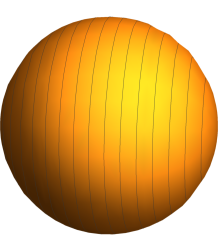
Figure 1: $\mathbb{C}\mathbb{P}^{1}$ with $r=1$

We note that the analysis above was classical, and the FI parameter runs in the quantum theory, and the $\mathbb{C}\mathbb{P}^{1}$ theory actually flows to a massive theory in the infra-red. In this paper we will mostly be interested in GLSMs that flow to 2d SCFTs in the infra-red (although we will make some comments on the $\mathbb{C}\mathbb{P}^{1}$ model in Section 5). Now, a necessary condition for the GLSM (5) to flow to a 2d SCFT (or equivalently, for the corresponding toric variety to be a Calabi-Yau manifold) is that there is a left- and right-moving chiral R-symmetry. For these chiral symmetries to be non-anomalous one has the condition:

$$\sum_{i}Q^{a}_{i}\;=\;0\,,\qquad a=1,\cdots,n-d\,.$$ (17)

As mentioned in the introduction, such a constraint on the charges cannot be satisfied by a compact toric variety. Our next three examples, as well as our main focus in the bulk of this paper, involve GLSMs described by the action (5) with the condition (17), which describe non-compact target spaces.

Example 2: ${\bf\mathbb{C}/\mathbb{Z}_{2}}$, $(n,d)=(2,1)$.

Our second example has two chiral superfields $\Phi_{1}$ and $\Phi_{2}$ with charges $Q_{i}=\pm 1$ respectively. The vacuum manifold is:

$$\quad V(r)=\{|\phi_{1}|^{2}-|\phi_{2}|^{2}=r\}/U(1)\,.$$ (18)

This is one dimensional complex space with a natural gauge invariant complex coordinate $M=\phi_{1}\phi_{2}$. We can obtain the (tree level) metric on $V$ by the symplectic quotient as before or, equivalently, by integrating out the gauge fields as we now show. At a generic point on the Higgs branch $M$ has a non-zero expectation value and the $U(1)$ gauge field $V_{\mu}$ gets a mass of order $e$. At lower energy scales, we can integrate out the gauge field by solving the classical equations of motion to obtain:

$$V_{\mu}\;=\;-\frac{1}{2}\,\frac{\sum_{i=1}^{2}Q_{i}\bigl{(}\overline{\phi}_{i}\partial_{\mu}\phi_{i}-\phi_{i}\partial_{\mu}\overline{\phi}_{i}\bigr{)}}{\sum_{i=1}^{2}Q_{i}^{2}|\phi_{i}|^{2}}\,.$$ (19)

Solving the D-term equation for $\phi_{1}$ and $\phi_{2}$ in terms of FI parameter $r$ and $M$, we obtain:

$$|\phi_{1}|^{2}\;=\;\frac{r}{2}+\sqrt{|M|^{2}+\frac{r^{2}}{4}},\qquad|\phi_{2}|^{2}\;=\;-\frac{r}{2}+\sqrt{|M|^{2}+\frac{r^{2}}{4}}$$ (20)

Substituting this in the action we get the non-linear sigma model with the target space metric

$$ds^{2}\;=\;\frac{dM\,d\overline{M}}{\sqrt{4M\,\overline{M}+r^{2}}}\,,$$ (21)

which can be derived from the Kähler potential

$$K\;=\;\sqrt{4M\,\overline{M}+r^{2}}-|r|\,{\rm arctanh}\Big{(}\frac{\sqrt{4M\,\overline{M}+r^{2}}}{|r|}\Bigr{)}\,.$$ (22)

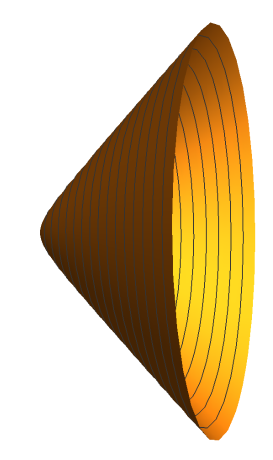
Figure 2: $\mathbb{C}/\mathbb{Z}_{2}$ with $r=2$

When the FI parameter $r$ vanishes the metric (21) is exactly that of $\mathbb{C}/\mathbb{Z}_{2}$ (i.e. as induced from the ambient complex plane). We can read off from the metric (21) that the FI parameter smoothes out the singularity near the tip $M=0$, but its effect dies out near the asymptotic region. It was observed in Aharony:2016jki that the elliptic genus of this model is exactly that of $\mathbb{C}$, prompting the conjecture that this GLSM flows from $\mathbb{C}/\mathbb{Z}_{2}$ (deformed by $r$ as above) to $\mathbb{C}$. We shall review the computation of the elliptic genus in the next section.

Example 3: $A_{1}$ space, $(n,d)=(3,2)$.

Our third example is a four-dimensional manifold modelled by three chiral superfields $\Phi_{i}$ and one gauge superfield. The charges of $\Phi_{i}$ are $(1,-2,1)$, respectively. The fields $X=\phi_{1}^{2}\phi_{2}$, $Y=\phi_{2}\phi_{3}^{2}$, $Z=\phi_{1}\phi_{2}\phi_{3}$ obey $XY=Z^{2}$, $X,Y,Z\in\mathbb{C}$, which is the algebraic equation of the $A_{1}$ space. We can solve the $D$-term equation

$$|\phi_{1}|^{2}-2|\phi_{2}|^{2}+|\phi_{3}|^{2}-r\;=\;0$$ (23)

by writing

$$\phi_{1}\;=\;\rho\cos\frac{\eta}{2}\,e^{i\theta_{1}}\,,\qquad\phi_{2}\;=\;\sqrt{\frac{\rho^{2}-r}{2}}\,e^{i\theta_{2}}\,,\qquad\phi_{3}\;=\;\rho\sin\frac{\eta}{2}\,e^{i\theta_{3}}\,,$$ (24)

where the angle $\eta$ has a periodicity of $\pi$. The angles $\psi_{1}=2\theta_{1}+\theta_{2}$, $\psi_{3}=2\theta_{3}+\theta_{2}$ are the arguments of the gauge invariant coordinates $X,Y\in\mathbb{C}$. Implementing the further $U(1)$ gauging by any of the two methods shown above, we obtain the tree-level metric. which coincides with the asymptotic form of the Eguchi-Hanson metric for $A_{1}=\mathbb{C}^{2}/\mathbb{Z}_{2}$. The full metric is not that of $A_{1}$ even when $r=0$, and only agrees with the ALE metric asymptotically. This can be immediately seen, for example, from the fact that the Ricci scalar curvature of this model only vanishes asymptotically.

The elliptic genus of this model was computed in Harvey:2014nha and it was found that it agrees with that of $\mathbb{C}^{2}/\mathbb{Z}_{2}$ (as we shall review in the next section). This leads to the natural conjecture that this GLSM flows from the metric (21) to $\mathbb{C}^{2}/\mathbb{Z}_{2}$, or more precisely the $A_{1}$ space resolved by the FI parameter $r$, i.e. the Eguchi-Hanson metric. We comment that $\mathcal{N}=(4,4)$ supersymmetric GLSMs for ALE spaces directly give the ALE hyperKähler metric in the UV, and there is no RG flow. This is a reflection of the enhanced supersymmetry.

This example can be easily generalized to all the $A_{k}$ models with $k$ gauge multiplets and $k+2$ chiral multiplets with charges $(1,-2,1,0,\cdots 0)$, $(0,1,-2,1,0,\cdots,0)$, $\cdots$, $(0,\cdots,0,1,-2,1)$. We shall not discuss more details of these models in this paper.

Example 4: Conifold, $(n,d)=(4,3)$.

Our final example is a six-dimensional manifold modelled by four chiral superfields $\Phi_{i}$ and one gauge superfield. The charges of $\Phi_{i}$ are $(+1,+1,-1,-1)$, respectively. The fields $X=\phi_{1}\phi_{3}$, $Y=\phi_{2}\phi_{4}$, $U=\phi_{1}\phi_{4}$, and $V=\phi_{2}\phi_{3}$ obey the algebraic equation of the conifold $XY=UV$. At the level of the metric the pattern is similar to the above two examples. The UV metric is asymptotically that of the conifold, deformed by the FI parameter $r$ which smoothes out the singularity near the tip. The Ricci tensor and Ricci scalar does not vanish when $r=0$, but approach zero asymptotically. We conjecture that this model flows to the conifold. We present the elliptic genus of this model in Section 3.

2.2 The squashing deformation

The GLSM (5) has, in addition to the $U(1)^{n-d}$ gauge symmetry, an independent global $U(1)^{d}$ flavor symmetry under which the chiral superfields carry some charges $F_{i}^{\ell}$, $\ell=1,\cdots,d$. The squashing deformation Hori:2001ax involves gauging this symmetry and simultaneously introducing a set of $d$ compensator chiral superfields which translate under the flavor gauge fields. The action of the squashed model has three changes compared to the action $S_{0}$ in (5). Firstly, one introduces a set of flavor gauge fields $V^{\prime}_{\ell}$, $\ell=1,\cdots,d$ with canonical kinetic terms

$$S_{1}\;=\;-\frac{1}{4\pi e^{\prime 2}}\int{\mathrm{d}}^{2}x\,\int{\mathrm{d}}^{4}\theta\sum_{\ell=1}^{d}\,\overline{\Sigma}^{\prime}_{\ell}\,\Sigma^{\prime}_{\ell}\,.$$ (25)

Secondly, the kinetic term of the chiral superfields in $S_{0}$ undergo the modification:

$$\sum_{a=1}^{n-d}Q_{i}^{a}V_{a}\;\rightarrow\;\sum_{a=1}^{n-d}Q_{i}^{a}V_{a}\,+\,\sum_{\ell=1}^{n}F_{i}^{\ell}V^{\prime}_{\ell}\,,$$ (26)

to give an action which we call $S^{\prime}_{0}$. Thirdly, one has the additional term in the action:

$$S_{2}\;=\;{1\over 2\pi}\int{\mathrm{d}}^{2}x\,\int{\mathrm{d}}^{4}\theta\,\sum_{\ell=1}^{d}\,{k_{\ell}\over 4}(P_{\ell}+\overline{P}_{\ell}+V^{\prime}_{\ell})^{2}\,.$$ (27)

The action of the squashed toric model is given by:

$$S_{\text{squashed}}\;=\;S^{\prime}_{0}+S_{1}+S_{2}\,.$$ (28)

The vacuum manifold of this theory is found by solving the constraint equations imposed by setting both $D$ and $D^{\prime}$ to zero:

$$D_{a}\;=\;-e_{a}^{2}\,\mu_{a}\,,\qquad\mu_{a}\;=\;\sum_{i=1}^{n}Q_{i}^{a}\,|\phi_{i}|^{2}-r_{a}\,,\qquad a=1,\dots,n-d\,,$$ (29)

$$D^{\prime}_{\ell}\;=\;-e^{\prime 2}\mu^{\prime}_{\ell},\qquad\mu^{\prime}_{\ell}\;=\;\sum_{i=1}^{n}F^{\ell}_{i}\,|\phi_{i}|^{2}+k\,\mbox{Re}P_{\ell},\qquad\ell=1,...,d\,.$$ (30)

The physically inequivalent vacua are given by

$$\widetilde{V}\;=\;\mu^{-1}(0)/(U(1)^{n-d}\times U(1)^{d})\,,\qquad\mu\;=\;(\mu_{a},\mu^{\prime}_{\ell})\,.$$ (31)

Thus we see that the vacuum manifolds of the squashed models—the squashed toric manifolds—are also toric manifolds with a local $U(1)^{d}$ action Hori:2001ax . We can choose to parameterize the base of the vacuum manifold of the squashed models by $\mbox{Re}P_{\ell}$ and, by a gauge choice, the circle fibres by $\mbox{Im}P_{\ell}$. In the interior of the base, where all the original gauge invariant coordinates are non-zero and finite, this circle has a fixed radius of order $\sqrt{k_{\ell}}$, whereas at the edges and corners (where one or more of the original gauge invariant coordinates are zero or infinity) some of the circles shrinks to zero size. An important difference with the unsquashed case is that even when the sum of the original gauge charges are zero, i.e. when the unsquashed vacuum manifold flows to a Calabi-Yau manifold, the squashed deformations break the Ricci-flat condition. Nevertheless the conjecture is that they flow to a $\mathcal{N}=(2,2)$ SCFT with a non-trivial dilaton profile.

We now illustrate some of the features of the squashed toric manifolds. We begin with the Kähler form of the free theory which can be read off from the action (28) to be (with $\phi_{i}=\rho_{i}e^{i\theta_{i}}$ as before):

$$\widetilde{\omega}\;=\;\omega+\frac{k}{2}\sum_{\ell=1}^{d}k_{\ell}\,\mbox{Re}p_{\ell}\wedge\text{Im}\,p_{\ell}\,,\qquad\omega\;=\;\sum_{i=1}^{n}\,\rho_{i}\,d\rho_{i}\wedge d\theta_{i}\,.$$ (32)

Here $\omega$ is the Kähler form of the unsquashed model written in terms of the original chiral fields before any gauging. The quotienting procedure can be done by using the differential of the $D$-term constraints (29), (30) to obtain

$$\widetilde{\omega}\;=\;\sum_{i=1}^{n}\,\rho_{i}\,d\rho_{i}\wedge d\widetilde{\theta}_{i}\,,\qquad\widetilde{\theta}_{i}\;=\;\theta_{i}-\sum_{\ell=1}^{d}F^{\ell}_{i}\,\text{Im}\,p_{\ell}\,,$$ (33)

and then expressing the $\rho_{i}$ in terms of the gauge-invariant coordinates $\widetilde{Z}_{\ell}$ of the squashed model.

It may be perhaps more instructive to perform the quotienting in two steps: the unsquashed model already comes with a set of coordinates $Z_{\ell}=Z_{\ell}(\{\phi_{i}\})$, $\ell=1,\cdots,d$ that are gauge-invariant with respect to the gauge transformations generated by $V_{a}$, $a=1,\cdots,n-d$ in terms of which the Kähler form can be written as:

$$\omega\;=\;\sum_{i,\overline{j}=1}^{d}\omega_{i\overline{j}}\,dZ_{i}\wedge d\overline{Z}_{\overline{j}}\,.$$ (34)

We can now do the squashing deformation, i.e. the gauging with respect to the fields $V^{\prime}_{\ell}$, for which a set of fully gauge-invariant coordinates is:

$$\widetilde{Z}_{\ell}\;=\;Z_{\ell}\Bigl{(}\bigl{\{}\phi_{i}\,\exp\bigl{(}-\sum_{\ell=1}^{d}F_{i}^{\ell}P_{\ell}\bigr{)}\bigr{\}}\Bigr{)}\,,\qquad\ell=1,\cdots,d\,,$$ (35)

where $Z_{\ell}(\{\phi_{i}\})$ are the gauge-invariant composite fields of the unsquashed model. We write $Z_{\ell}=R_{\ell}\,e^{i\psi_{\ell}}$ and $\widetilde{Z}_{\ell}=\widetilde{R}_{\ell}\,e^{i\widetilde{\psi}_{\ell}}$.

We now illustrate this in the simple example of the squashed $\mathbb{C}\mathbb{P}^{1}$ model for which the vacuum manifold is:

$$\quad\widetilde{V}(r)\;=\;\{|\phi_{1}|^{2}+|\phi_{2}|^{2}=r\,,\;F_{1}|\phi_{1}|^{2}+F_{2}|\phi_{2}|^{2}=-k\,\mbox{Re}P\}/(U(1)\times U(1))\,.$$ (36)

The complex coordinate $Z=(\phi_{1}/\phi_{2})=R\,e^{i\psi}$ is the gauge-invariant coordinate of the unsquashed model, and $\widetilde{Z}=Ze^{(F_{2}-F_{1})P}$ is the corresponding coordinate of the squashed model invariant under both the $U(1)$ gauge transformations. As explained in the previous section, the Kähler form of the unsquashed model is (using the differential of the D-term constraint):

$$\omega\;=\;\sum_{i=1}^{2}\rho_{i}\,d\rho_{i}\wedge d\theta_{i}\;=\;\rho_{1}\,d\rho_{1}\wedge d\psi\,\;=\;r\,\frac{R\,dR\wedge d\psi}{(1+R^{2})^{2}}\,.$$ (37)

The Kähler form of the corresponding squashed model is

$$\widetilde{\omega}\ =\omega+\frac{k}{2}\,k\,\mbox{Re}p\wedge\text{Im}\,p\;=\;\rho_{1}\,d\rho_{1}\wedge d\widetilde{\psi}\;=\;r\,\frac{R\,dR\wedge d\widetilde{\psi}}{(1+R^{2})^{2}}$$ (38)

where we have used the differential of the $D^{\prime}$-term constraint in writing the second equality.

We now want to convert everything to $\widetilde{Z}$, $\overline{\widetilde{Z}}$ or, equivalently, $\widetilde{R}$ and $\widetilde{\psi}$, for which we use the trick of Appendix C to convert the coordinate $R$ to the coordiante $\widetilde{R}(R)$. In this manner we find the corresponding metric to be:

$$ds^{2}\;=\;r\,\frac{R}{(1+R^{2})^{2}}\,\biggl{(}\frac{\widetilde{R}^{\prime}(R)}{\widetilde{R}(R)}dR^{2}+\frac{\widetilde{R}(R)}{\widetilde{R}^{\prime}(R)}d\widetilde{\psi}^{2}\biggr{)}\,.$$ (39)

Computing the derivative we obtain

$$\frac{1}{\widetilde{R}}\frac{d\widetilde{R}}{dR}\;=\;\frac{2(F1-F2)^{2}rR^{2}+k(1+R^{2})^{2}}{kR(1+R^{2})^{2}}\;=\;\frac{2rR^{2}+\widehat{k}(1+R^{2})^{2}}{\widehat{k}R(1+R^{2})^{2}}\,,$$ (40)

where $\widehat{k}=k/(F_{1}-F_{2})^{2}$. The metric is then given by

$$ds^{2}\;=\;\frac{r(2rR^{2}+\widehat{k}(1+R^{2})^{2})}{\widehat{k}(1+R^{2})^{4}}\,dR^{2}+\frac{\widehat{k}rR^{2}}{2R^{2}r\,+\,\widehat{k}(1+R^{2})^{2}}d\psi^{2}\,,$$ (41)

which has the shape of a sausage Fateev:1992tk ; Fendley:1992dm .

Now we briefly discuss the squashed $\mathbb{C}/\mathbb{Z}_{2}$ model. The vacuum equations for this model are:

$$\quad\widetilde{V}(r)\;=\;\{|\phi_{1}|^{2}-|\phi_{2}|^{2}=r\,,\;F_{1}|\phi_{1}|^{2}+F_{2}|\phi_{2}|^{2}=-k\,\text{Re}P\}/(U(1)\times U(1))\,.$$ (42)

This is a one dimensional complex space with natural gauge invariant complex coordinate $M=\phi_{1}\phi_{2}\,e^{{-(F_{1}+F_{2})P}}$. At a generic point on the Higgs branch labelled by the vacuum expectation value of $M$, both the gauge fields $V_{\mu}$ and $V^{\prime}_{\mu}$ are massive and therefore, at the energy scale below the masses of the gauge fields, we can integrate them out to get the non linear sigma model. Solving for the equations of motion for the gauge fields $V_{\mu}$ and $V^{\prime}_{\mu}$, one obtains

$$V_{\mu}\;=\;\frac{r_{1}^{2}\,\partial_{\mu}\theta_{1}-r_{2}^{2}\partial_{\mu}\theta_{2}+(F_{2}r_{2}^{2}-F_{1}r_{1}^{2})V^{\prime}_{\mu}}{r_{1}^{2}+r_{2}^{2}}\,,$$ (43)

where

$$V^{\prime}_{\mu}\;=\;\frac{(r_{1}^{2}+r_{2}^{2})\,k\,\partial_{\mu}\text{Im}P+2b_{1}\,r_{1}^{2}\,r_{2}^{2}\,(\partial_{\mu}\theta_{1}+\partial_{\mu}\theta_{2})}{2r_{1}^{2}\,r_{2}^{2}\,b_{1}^{2}+(r_{1}^{2}+r_{2}^{2})\,k}\,.$$ (44)

Here $\phi_{1}\;=\;r_{1}e^{i\theta_{1}},\,\phi_{2}\;=\;r_{2}e^{i\theta_{2}}$ and $b_{1}\;=\;F_{1}+F_{2}$.

Substituting the above expressions for the gauge fields in the kinetic part of the Lagrangian

$$|D_{\mu}\phi_{1}|^{2}+|D_{\mu}\phi_{2}|^{2}+\frac{k}{2}|D_{\mu}P|^{2}\,,$$ (45)

and also using the $D$ and $D^{\prime}$ constraints equations to eliminate $\text{Re}P$ and $r_{2}$ in terms of $r_{1}$ and $r$, we obtain the tree-level UV metric of the squashed $\mathbb{C}/\mathbb{Z}_{2}$:

$$ds^{2}\;=\;\frac{(2\rho^{2}+\widetilde{k}\sqrt{4\rho^{2}+r^{2}})}{\widetilde{k}\,(4\rho^{2}+r^{2})}\,d\rho^{2}\,+\,\frac{\widetilde{k}\,\rho^{2}}{(2\rho^{2}+\widetilde{k}\sqrt{4\rho^{2}+r^{2}})}\,d\psi^{2}\,,$$ (46)

where $\rho=r_{1}r_{2}\;=\;r_{1}\sqrt{r_{1}^{2}-r}$, and $\psi=\theta_{1}+\theta_{2}-b_{1}\text{Im}P$. The metric depends on the FI parameter, $r$, and $\widetilde{k}$ which is the ratio of $k$ and $b^{2}_{1}$, $\widetilde{k}=k/b_{1}^{2}$.

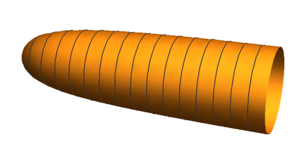
Figure 4: Squashed $\mathbb{C}/\mathbb{Z}_{2}$ with $\tilde{k}=1$ and $r=1$

The unsquashed vacuum manifold is $\mathbb{C}/\mathbb{Z}_{2}$ which has been smoothed near the tip. The squashed manifold, in contrast, has a cigar-like shape. The circle which grows without bound has been squashed so as to give an asymptotic cylinder. We shall see in Section 4 that the elliptic genus of the squashed $\mathbb{C}/\mathbb{Z}_{2}$ is exactly that of the cigar manifold, based on which we conjecture that the GLSM for squashed $\mathbb{C}/\mathbb{Z}_{2}$ describes an RG flow from (46) to the cigar SCFT.

Similarly the squashed ALE space and the squashed conifold have a shape which can be described as a higher-dimensional cigar, i.e. a $(2d-1)$-dimensional sphere fibered over the radial direction in a manner that the radius of the sphere asymptotes to a constant. These are similar to the manifolds described in Hori:2002cd , but again the details are slightly different. We conjecture that the IR fixed points where they flow to are the same as that of Hori:2002cd , namely the IR SCFT reached by the theory on NS5-branes wrapped on certain compact manifolds. Our elliptic genus computations of these models in Section 4 may thus have possible applications to the gauge theories living on such brane configurations.

3 Elliptic genus of toric sigma models

In this section we review the path integral derivation of the elliptic genus of toric sigma models, and illustrate it with the examples discussed in the previous section. As mentioned in the introduction the elliptic genus is the partition function of the GLSM on a two-dimensional flat torus with periodic boundary conditions on fermions and bosons, with background R-symmetry gauge field $A^{R}_{\mu}$ and background flavor symmetry gauge field $V^{\prime}_{\mu}$ which couple to the dynamical fields through covariant derivatives.

In the previous section we saw that the $d$-dimensional toric manifold is labelled by the gauge invariant complex coordinates $Z_{\ell}$, $\ell=1,\cdots,d$. The toric manifold has a non-trivial $U(1)^{d}$ action which is diagonalized by $Z_{\ell}$ transforming as $Z_{\ell}\rightarrow e^{i\phi_{\ell}}Z_{\ell}$. For each of these $U(1)$s we will associate a chemical potential $v_{\ell}$ which couples to the corresponding conserved current. As we shall see below the elliptic genus of the toric manifold depends only on the parameters $\tau$, $z$, and $v_{\ell}$.

We focus on the theories of the type discussed in the previous section, namely $\mathcal{N}=(2,2)$ supersymmetric gauge theory with gauge group $U(1)^{n-d}$ coupled to $n$ chiral multiplets. In order to compute the elliptic genus we need conserved left and right-moving $U(1)$ R-symmetries. These are the theories that obey the Calabi-Yau condition and flow to $\mathcal{N}=(2,2)$ SCFTs. From our discussion in the previous section, this means that we have to restrict our attention to the non-compact models. We shall return to a compact example in Section 5 and compute its Witten index.

We denote the gauge charges of the chiral multiplets by $Q_{i}^{a}$, $i=1,\cdots,n$, $a=1,\cdots,n-d$, and the flavor charges by $F_{i}^{\ell}$, $\ell=1,\cdots,d$. The computation of the partition function depends on the holonomies

$$u^{a}\;=\;\oint_{A}V^{a}-\tau\oint_{B}V^{a}\,,\qquad u^{\prime\ell}\;=\;\oint_{A}V^{\prime\ell}-\tau\oint_{B}V^{\prime\ell}\,,\qquad z\;=\;\oint_{A}A^{R}-\tau\oint_{B}A^{R}\,,$$ (47)

along the two cycles of the torus, which we collectively denote as $u,u^{\prime},z,$ respectively. The large gauge transformation symmetries of the gauge fields imply that the complex parameters $u^{a},u^{\prime\ell}$, and $z$ take values in $\mathbb{E}_{\tau}=\mathbb{C}/(\mathbb{Z}\tau+\mathbb{Z})$. The chemical potentials $v_{\ell}$ are linear combinations of the $u^{\prime}_{\ell}$s determined by the corresponding gauge-invariant composite fields built out of the chiral multiplets $\phi_{i}$.

The elliptic genus of such a GLSM was computed in Benini:2013nda ; Benini:2013xpa using the technique of supersymetric localization. The localization technique reduces the path integral to an integral over the localization manifold which is the set of solutions to the off-shell BPS equations of the right-moving supercharge $Q$. The localization manifold in this case is labelled by arbitrary values of the holonomies $u^{a}\in E_{\tau}$ of the gauge fields and all other fields set to zero. The classical action of the theory on this manifold vanishes and thus the integrand reduces to a one-loop determinant of the quadratic fluctuations of a certain deformation called the localizing action. In this case the one loop determinant (with zero modes removed) is

$$Z_{\text{1-loop}}(\tau,z,u,u^{\prime})\;=\;\biggl{(}\frac{-i\,\eta(\tau)}{\vartheta_{1}(\tau,z)}\biggr{)}^{n-d}\,\prod_{i=1}^{n}\frac{\vartheta_{1}(\tau,(\frac{R_{i}}{2}-1)z+Q_{i}\cdot u+F_{i}\cdot u^{\prime})}{\vartheta_{1}(\tau,\frac{R_{i}}{2}z+Q_{i}\cdot u+F_{i}\cdot u^{\prime})}\,.$$ (48)

The first factor in the above expression comes from the one loop computation of the vector multiplets and the second factor comes from the chiral multiplets. Here we have introduced the notation

$$Q_{i}\cdot u\;=\;\sum_{a=1}^{n-d}Q^{a}_{i}\,u^{a}\,,\qquad F_{i}\cdot u^{\prime}\;=\;\sum_{\ell=1}^{d}F^{\ell}_{i}\,u^{\prime\ell}\,.$$ (49)

In the above formula $R_{i}$ is the vector R-charge of the boson in the $i$th chiral multiplet. As we do not have any superpotential in our theories, we can shift $R_{i}$ by the linear combinations of the gauge and flavor symmetries to set it to zero. In the following discussion, we will assume that the R-charges of all the chiral multiplets are zero, they can be reinstated easily in all our formulas.

The one loop determinant $Z_{\text{1-loop}}(\tau,z,u,u^{\prime})$ has poles in $u\in\mathbb{C}^{n-d}$, along certain hyperplanes defined by the condition that one or more chiral multiplets become massless which is given by

$$Q_{i}\cdot u+F_{i}\cdot u^{\prime}=0\,\quad\text{mod}\,\,\mathbb{Z}\tau+\mathbb{Z}\,.$$ (50)

The integral over $u$ reduces to computing the residues of $Z_{\text{1-loop}}(\tau,z,u,u^{\prime})$ at the set of poles $\mathfrak{M}_{\text{sing}}$ where $m$ ($m\geq n-d$) of these hyperplanes intersect. The partition function is then given by

$$\chi_{\text{ell}}(M_{\text{tor}};\tau,z,u^{\prime})\;=\;-\sum_{u_{*}\in\mathfrak{M^{*}}_{\text{sing}}}\underset{u=u_{*}}{\text{JK-Res}}(Q(u_{*}),\eta)\,Z_{\text{1-loop}}(\tau,z,u,u^{\prime})\,,$$ (51)

where $\text{JK-Res}(Q(u_{*}),\eta)$ is a residue operation in $(n-d)$ complex dimensions called the Jeffrey-Kirwan residue Jeffrey:9307 ; Benini:2013xpa . Here $\eta$ is an arbitrary vector in $\mathbb{R}^{n-d}$ needed to define this residue operation, although the final result does not depend on the choice of such a vector. For each $u\in\mathfrak{M}_{\text{sing}}$, $Q(u)$ is the set of (at least $n-d$) charges defining the hyperplanes intersecting at $u$. The set $\mathfrak{M^{*}}_{\text{sing}}$ is the subset of $\mathfrak{M}_{\text{sing}}$ defined by the condition that, for any point $u^{*}\in\mathfrak{M^{*}}_{\text{sing}}$, the vector $\eta$ is contained in the cone generated by $(n-d)$ linearly independent charge vectors in $Q(u_{*})$.

We will now review the modular and elliptic properties of the expression (51). We will then illustrate the formula (51) using the examples discussed in Section 2. The first example $\mathbb{C}\mathbb{P}^{1}$ does not have an anomaly-free R-symmetry and therefore the expression (2) for the elliptic genus is not well defined. The other three examples $\mathbb{C}/\mathbb{Z}_{2}$, ALE space, and the conifold do have a conserved R-symmetry and we proceed to discuss them in turn.

3.1 Modular and elliptic properties

The function $\chi_{\text{ell}}(M_{\text{tor}};\tau,z,u^{\prime})$ is holomorphic in $z$ and meromorphic in the $u^{\prime\ell}$ variables. We now show that it is a Jacobi form in $d+1$ elliptic variables $(z,u^{\prime 1},\cdots,u^{\prime d})$ (and one modular variable $\tau$) with weight $0$ and index

$$M\;=\;\begin{pmatrix}d/2&-b_{1}/2&\cdots&-b_{d}/2\\ -b_{1}/2&0&\cdots&0\\ \cdots&0&\cdots&0\\ -b_{d}/2&0&\cdots&0\\ \end{pmatrix}\,,$$ (52)

that is  $M_{zz}=d/2$, $M_{zu^{\prime}_{\ell}}=-b_{\ell}/2$, and the rest of the entries are zero. For future use we denote the sum of the flavor charges for each flavor symmetry as:

$$b_{\ell}\;=\;\sum_{i=1}^{n}F^{\ell}_{i}\,.$$ (53)

For the definition of multivariable Jacobi forms see Appendix A.

The function $Z_{\text{1-loop}}(\tau,z,u,u^{\prime})$ transforms as follows:

1. Under the elliptic transformation of the variable $z$ with the other elliptic variables $u^{\prime\ell}$ fixed we have (using the CY condition $\sum_{i=1}^{n}Q_{i}^{a}=0$):

   $$Z_{\text{1-loop}}(\tau,z+\lambda\tau+\mu,u,u^{\prime})\;=\;e^{-2\pi i\left(\frac{d}{2}\lambda^{2}\,\tau+\lambda(z\,d-\sum_{\ell=1}^{d}\,b_{\ell}\,u^{\prime\ell})\right)}\,Z_{\text{1-loop}}(\tau,z,u,u^{\prime}),\quad\lambda,\mu\in\mathbb{Z}\,.$$ (54)

2. Under the elliptic transformation of the variable $u^{\prime\ell}$ with $z$ fixed ,

   $$Z_{\text{1-loop}}(\tau,z,u,u^{\prime\ell}+\lambda^{\ell}\tau+\mu^{\ell})\;=\;e^{2\pi iz\sum_{\ell=1}^{d}b_{\ell}\,\lambda^{\ell}}\,Z_{\text{1-loop}}(\tau,z,u,u^{\prime})\,.$$ (55)

We can now deduce the elliptic transformation of the function $\chi_{\text{ell}}(M_{\text{tor}};\tau,z,u^{\prime})$ using these identities. Firstly, under the shift of $z$ as $z\rightarrow z+\lambda\tau+\mu$ keeping $u^{\prime\ell}$ fixed, the locations of the poles in the function $Z_{\text{1-loop}}(\tau,z,u,u^{\prime})$ remain unchanged. Therefore one can pull out the phase in the JK residue operation to obtain

$$\chi_{\text{ell}}(M_{\text{tor}};\tau,z+\lambda\tau+\mu,u^{\prime})$$

$$\qquad\qquad\;=\;-\sum_{u_{*}\in\mathfrak{M^{*}}_{\text{sing}}}\underset{u=u_{*}}{\text{JK-Res}}(Q(u_{*}),\eta)e^{-2\pi i\left(\frac{d}{2}\lambda^{2}\tau+\lambda(zd-\sum_{\ell=1}^{d}b_{\ell}u^{\prime\ell})\right)}Z_{\text{1-loop}}(\tau,z,u,u^{\prime})$$

$$\qquad\qquad\;=\;e^{-2\pi i\left(\frac{d}{2}\lambda^{2}\tau+\lambda(zd-\sum_{\ell=1}^{d}b_{\ell}u^{\prime\ell})\right)}\chi_{\text{ell}}(M_{\text{tor}};\tau,z,u^{\prime})\,.$$ (56)

Under the other elliptic transformations $u^{\prime\ell}$ as $u^{\prime\ell}\rightarrow u^{\prime\ell}+\lambda^{\ell}\tau+\mu^{\ell}$ with $z$ fixed. The locations of poles of $Z_{1-\text{loop}}$ change from (50) to

$$Q_{i}(u_{*})+F_{i}(u^{\prime})+\sum_{\ell=1}^{d}F^{\ell}_{i}(\lambda^{\ell}\tau+\mu^{\ell})\;=\;0\quad\text{mod}\,\,\mathbb{Z}\tau+\mathbb{Z}\,.$$ (57)

Since $F_{i}^{\ell}\in\mathbb{Z}$, we see that the set of poles in $E_{\tau}=\mathbb{C}/\mathbb{Z}\tau+\mathbb{Z}$ does not change, although the individual poles may get rearranged. Thus we get

$$\chi_{\text{ell}}(M_{\text{tor}};\tau,z,u^{\prime\ell}+\lambda^{\ell}\tau+\mu^{\ell})\;=\;e^{2\pi iz\sum_{\ell=1}^{d}b_{\ell}\lambda^{\ell}}\chi_{\text{ell}}(M_{\text{tor}};\tau,z,u^{\prime})\,.$$ (58)

As we will see later this condition is essential in order to gauge the flavor symmetry.

The modular transformation property of $Z_{\text{1-loop}}$ applied to Formula (51) yields the modular transformation of $\chi_{\text{ell}}(M_{\text{tor}})$. Putting this together with the above elliptic transformation properties, we see that $\chi_{\text{ell}}(M_{\text{tor}};\tau,z,u^{\prime})$ is a Jacobi form with weight $0$ and index $M$.

3.2 Examples

We now illustrate the considerations above in the examples that we introduced in Section 2. As explained above the elliptic genus is only well-defined for the non-compact examples. In each case the elliptic genus is a Jacobi form holomorphic in $z$ and meromorphic in $v_{\ell}$, $\ell=1,\cdots,d$. This is consistent with the fact that $v_{\ell}$ is chemical potential for the rotation of the gauge-invariant complex variable $Z_{\ell}$. The basic model for the meromorphicity in the flavored elliptic genus is the complex plane $\mathbb{C}$. The pole arises from the bosonic zero mode on the plane. The divergence is regularized by the chemical potential for flavor rotation, i.e. the angular momentum of the plane whose fixed point is the origin of $\mathbb{C}$. The poles in our expressions can thus be associated with the fixed points of the $U(1)^{d}$ symmetries.

We note that the FI term which smooths out the orbifold singularities (see e.g. the discussion around Figure 2 for the case $\mathbb{C}/\mathbb{Z}_{2}$) is a $Q$-exact term and therefore does not affect our computation of the elliptic genus.

$\mathbb{C}/\mathbb{Z}_{2}$ (flowing to $\mathbb{C}$)

We consider the $U(1)$ gauge theory with 2 chiral multiplets $\Phi_{1}$ and $\Phi_{2}$ with gauge charges $1,-1$, respectively and flavor charges $F_{1},F_{2}$, respectively. This model describes the space $\mathbb{C}/\mathbb{Z}_{2}$ which is expected to flow to $\mathbb{C}$. In the $U(1)$ case the Jeffrey-Kirwan residue operation in (51) reduces to collecting the residue from the poles $u_{i}$ satisfying the condition $\eta Q>0$, where $Q$ is the charge of the chiral multiplet becoming massless at $u$. Therefore, choosing the vector $\eta>0$, we obtain

$$\chi_{\text{ell}}(\mathbb{C};\tau,z,u^{\prime})\;=\;-\sum_{u_{j}\in\mathfrak{M}_{\text{sing}}^{+}}\oint_{u=u_{j}}{\mathrm{d}}u\frac{i\eta(q)^{3}}{\vartheta_{1}(\tau,-z)}\frac{\vartheta_{1}(\tau,-z+u+F_{1}u^{\prime})}{\vartheta_{1}(\tau,u+F_{1}u^{\prime})}\frac{\vartheta_{1}(\tau,-z-u+F_{2}u^{\prime})}{\vartheta_{1}(\tau,-u+F_{2}u^{\prime})}\,.$$ (59)

Here $F_{i}$ are flavor charges of the chiral multiplets. In the present case, we have only one pole, and for a generic value of $u^{\prime}$ the location of the pole is given by $u+F_{1}u^{\prime}=0\,(\text{mod}\,\,\mathbb{Z}+\tau\mathbb{Z})$. Using the residue formula (122) we obtain

$$\chi_{\text{ell}}(\mathbb{C};\tau,z,u^{\prime})\;=\;\frac{\vartheta_{1}(\tau,-z+(F_{1}+F_{2})u^{\prime})}{\vartheta_{1}(\tau,(F_{1}+F_{2})u^{\prime})}\;=\;\frac{\vartheta_{1}(\tau,-z+v)}{\vartheta_{1}(\tau,v)}\,,$$ (60)

where $v=b_{1}u^{\prime}$, with $b_{1}=(F_{1}+F_{2})$, the flavor charge of the gauge invariant variable $Z=\phi_{1}\phi_{2}$. The expression (60) is equal to the elliptic genus of the $c=3$ superconformal field theory on $\mathbb{C}$ , with a chemical potential for the rotation of the complex coordinate $Z\in\mathbb{C}$. The function $\chi_{\text{ell}}(\mathbb{C};\tau,z,u^{\prime})$ is a meromorphic Jacobi form, with only one pole in $E_{\tau}$ at $v=0$, of weight $0$ and index

$$M_{\mathbb{C}}\;=\;\begin{pmatrix}1/2&-b_{1}/2\\ -b_{1}/2&0\end{pmatrix}\,.$$ (61)

$\text{Resolved}\,A_{1}\text{-Space}$

We consider the $U(1)$ gauge theory with 3 chiral multiplets $\Phi_{1}$, $\Phi_{2}$, and $\Phi_{3}$ with charges $1,-2,1$, respectively. There is a $U(1)^{2}$ flavor symmetry under which the chiral multiplets $\Phi_{i}$ have charges $F_{i}^{\ell},\,(\ell=1,2;\,i=1,2,3)$. This model describes the $ALE$ space of type $A_{1}$. We compute the Jeffrey-Kirwan residue by choosing the vector $\eta>0$, for which we pick up residues at poles $u=-F_{1}\cdot u^{\prime}$ and $u=-F_{3}\cdot u^{\prime}$. The elliptic genus is then given by

$$\chi_{\text{ell}}(A_{1};\tau,z,u^{\prime}) \;=\; \frac{\vartheta_{1}(\tau,-z+(F_{3}-F_{1})\cdot u^{\prime})}{\vartheta_{1}(\tau,(F_{3}-F_{1})\cdot u^{\prime})}\frac{\vartheta_{1}(\tau,-z+(2F_{1}+F_{2})\cdot u^{\prime})}{\vartheta_{1}(\tau,(2F_{1}+F_{2})\cdot u^{\prime})}$$

$$\qquad+\frac{\vartheta_{1}(\tau,-z+(F_{1}-F_{3})\cdot u^{\prime})}{\vartheta_{1}(\tau,(F_{1}-F_{3})\cdot u^{\prime})}\frac{\vartheta_{1}(\tau,-z+(2F_{3}+F_{2})\cdot u^{\prime})}{\vartheta_{1}(\tau,(2F_{3}+F_{2})\cdot u^{\prime})}$$

$$\;=\; \frac{\vartheta_{1}(\tau,-z+v_{2}-v_{1})}{\vartheta_{1}(\tau,v_{2}-v_{1})}\frac{\vartheta_{1}(\tau,-z+2v_{1})}{\vartheta_{1}(\tau,2v_{1})}+\frac{\vartheta_{1}(\tau,-z+v_{1}-v_{2})}{\vartheta_{1}(\tau,v_{1}-v_{2})}\frac{\vartheta_{1}(\tau,-z+2v_{2})}{\vartheta_{1}(\tau,2v_{2})}\,.$$

Here $2v_{1}=(2F_{1}+F_{2})\cdot u^{\prime}$ and $2v_{2}=(2F_{3}+F_{2})\cdot u^{\prime}$, which are the chemical potentials coupling to the rotations of the gauge invariant variables $X=\phi_{1}^{2}\phi_{2}$, and $Y=\phi_{3}^{2}\phi_{2}$. The Witten index, i.e. the value of the elliptic genus (3) at $z=0$ equals 2, which is exactly the Euler character of the Eguchi-Hanson space Eguchi:1978gw . The function $\chi_{\text{ell}}(A_{1};\tau,z,u^{\prime})$ is a meromorphic Jacobi form of weight $0$ and index

$$M_{A_{1}}\;=\;\begin{pmatrix}1&-b_{1}/2&-b_{2}/2\\ -b_{1}/2&0&0\\ -b_{2}/2&0&0\end{pmatrix}$$ (63)

in the variables $(z,u_{1}^{\prime},u_{2}^{\prime})$ with poles at $v_{1}(\{u^{\prime}_{\ell}\})=0$ and $v_{2}(\{u^{\prime}_{\ell}\})=0$.

Conifold

We consider the $U(1)$ gauge theory with 4 chiral multiplets $\Phi_{1}$,$\Phi_{2}$,$\Phi_{3}$ and $\Phi_{4}$ with charges $1,1,-1,-1$, respectively. This model describes the resolved conifold. There is a $U(1)^{3}$ flavor symmetry under which the chiral multiplets $\Phi_{i}$ have charges $F_{i}^{\ell},\,(\ell=1,2,3;\,i=1,2,3,4)$. Computing the Jeffrey-Kirwan residue as in the previous case and picking up the residues at the poles for $\eta<0$ (corresponding to the negative charge), we obtain

$$\chi_{\text{ell}}(\text{Conifold};\tau,z,u^{\prime}) \;=\; -\frac{\vartheta_{1}(\tau,-z+v_{1})}{\vartheta_{1}(\tau,v_{1})}\frac{\vartheta_{1}(\tau,-z+v_{3})}{\vartheta_{1}(\tau,v_{3})}\frac{\vartheta_{1}(\tau,-z+v_{2}-v_{1})}{\vartheta_{1}(\tau,v_{2}-v_{1})}$$

$$\quad-\frac{\vartheta_{1}(\tau,-z+v_{2})}{\vartheta_{1}(\tau,v_{2})}\frac{\vartheta_{1}(\tau,-z+v_{2}-v_{1}+v_{3})}{\vartheta_{1}(\tau,v_{2}-v_{1}+v_{3})}\frac{\vartheta_{1}(\tau,-z+v_{1}-v_{2})}{\vartheta_{1}(\tau,v_{1}-v_{2})}\,.$$

Here $v_{1}=(F_{1}+F_{3})\cdot u^{\prime}$, $v_{2}=(F_{1}+F_{4})\cdot u^{\prime}$ and $v_{3}\;=\;(F_{2}+F_{3})\cdot u^{\prime}$, which are the chemical potentials coupling to the rotations of the gauge invariant variables $X=\phi_{1}\phi_{3}$, $U=\phi_{1}\phi_{4}$ and $V=\phi_{2}\phi_{3}$. Again we see that the the elliptic genus is a meromorphic Jacobi form with index given by (52). The poles are at $v_{\ell}=0$, $\ell=1,2,3$, and $v_{4}=v_{2}+v_{3}-v_{1}=0$. These four poles correspond to the fixed points of $X$, $V$, $U$, and $Y=\phi_{2}\phi_{4}$ which obey $XY=UV$.

4 Elliptic genus of squashed toric sigma models

In this section we compute the elliptic genus of the squashed toric sigma models discussed in Section 2, and derive the main formula of the paper. The starting point is the unsquashed theory discussed in Section 3, namely the $U(1)^{n-d}$ gauge theory coupled to $n$ chiral multiplets. This theory has a $U(1)^{d}$ flavor symmetry, under which the chiral multiplets have charges $F_{i}^{\ell}$, $(i=1,\cdots,n,\ell=1,\cdots,d)$. The squashing corresponds to gauging the $U(1)^{d}$ symmetry and introducing $d$ compensator $P$-fields, as discussed in Section 2.2. The action of the theory is given in Equation (28). The details of the Lagrangian in the component form is given in Appendix D.

We use localization to compute the supersymmetric partition function of these theories. The main idea of the computation is very close to that of Benini:2013nda , Murthy:2013mya , which we follow. The first step is to deform the action by a $Q$-exact term with a coupling $\lambda$. The $Q$-exactness implies that the answer is independent of the coupling and we can therefore evaluate the path integral in the limit $\lambda\to\infty$. In this limit the path-integral reduces to the critical points of the deformation action, the localization manifold, and the computation of its one-loop determinant at these points. We choose the deformation such that the localization manifold is the set of solutions to the off-shell BPS equations of the supercharge $Q$ on the vector and chiral multiplets. This is given by the constant gauge field holonomies along the two cycles of $T^{2}$. As in the previous section we denote the holonomies of the $U(1)^{n-d}$ gauge fields and the $U(1)^{d}$ flavor gauge fields by $\{u^{a}\}_{a=1,..,n-d}$ and $\{u^{\prime\ell}\}_{\ell=1,..,d}$, respectively. The full functional integral reduces to an integral over these holonomies as well as the full field space of the compensator multiplets. Noting that the full Lagrangian for the $P$-multiplet fields evaluated on this above localization locus is quadratic, we can simply perform the Gaussian path-integral.

The one loop determinant coming from the integration over non zero modes for each vector multiplet is identical and is given by $\dfrac{i\eta(\tau)^{3}}{\vartheta_{1}(\tau,-z)}$, thus giving the following total contribution from the non zero modes of $n$ vector multiplets:

$$Z_{\text{vec}}(\tau,z)\;=\;\left(-\frac{i\eta(\tau)^{3}}{\vartheta_{1}(\tau,z)}\right)^{n}\,.$$ (65)

However this is not the complete result for the vector multiplet as there are zero modes of kinetic operator for gaugino fields $(\overline{\lambda}_{a+}^{(0)},\lambda_{a+}^{(0)})$ and $(\overline{\lambda}^{{}^{\prime}(0)}_{\ell+},\lambda_{\ell+}^{{}^{\prime}(0)})$. The zero modes $(\overline{\lambda}_{a+}^{(0)},\lambda_{a+}^{(0)})$ couple to chiral multiplets through Yukawa interactions and the zero modes $(\overline{\lambda}^{{}^{\prime}(0)}_{\ell+},\lambda_{\ell+}^{{}^{\prime}(0)})$ couple to both chiral and P-multiplets. As we see below the zero modes $(\overline{\lambda^{\prime}}^{(0)}_{+},\lambda_{+}^{{}^{\prime}(0)})$ are absorbed by the zero modes of the $P$-multiplet fermions $(\overline{\chi}_{\ell-}^{(0)},\chi_{\ell-}^{(0)})$ and the fermion zero modes $(\overline{\lambda}_{a+}^{(0)},\lambda_{a+}^{(0)})$ are absorbed by the Yukawa interactions of chiral multiplets. For details of the Lagrangian involving chiral, vector and $P$-multiplets, see Appendix D.

We first integrate over the fields in the $P_{\ell}$-multiplets whose Lagrangian is:

$$\frac{k_{\ell}}{2}\Big{(}-D^{{}^{\prime}\mu}\overline{p}_{\ell}D^{\prime}_{\mu}p_{\ell}+i\overline{\chi}_{\ell-}(\partial_{0}+\partial_{1})\chi_{\ell-}+i\overline{\chi}_{\ell+}(\partial_{0}-\partial_{1})\chi_{\ell+}+iD^{\prime}_{\ell}(p_{\ell}+\overline{p}_{\ell})+|F_{p_{\ell}}|^{2}$$

$$-|\sigma^{\prime}_{\ell}|^{2}+i\chi_{\ell+}\lambda^{\prime}_{\ell-}-i\chi_{\ell-}\lambda^{\prime}_{\ell+}+i\overline{\chi}_{\ell+}{\overline{\lambda}^{\prime}}_{\ell-}-i\overline{\chi}_{\ell-}{\overline{\lambda}}^{\prime}_{\ell+}\Big{)}\,.$$ (66)

The integration over the non zero modes of $\chi_{\ell\pm}$ gives

$$\prod_{m,n\in\mathbb{Z}}(m\tau+n+z)\prod_{m,n\in\mathbb{Z}\setminus(0,0)}(n+m\overline{\tau})\,,$$ (67)

and the integration over the non zero modes of $\text{Re}\,p_{\ell}$ gives

$$\prod_{m,n\in\mathbb{Z}\setminus(0,0)}|(n+m\tau)|\,.$$ (68)

Next we need to integrate over $\text{Im}\,p_{\ell}$. Since $\text{Im}\,p_{\ell}$ lives on a circle of unit radius, its mode expansion is given by

$$\text{Im}\,p_{\ell}\;=\;2\pi(w_{\ell}\sigma_{1}+m_{\ell}\sigma_{2})+\text{Im}\,p_{\ell\text{oscil}},$$ (69)

where $\sigma_{1,2}$ are coordinates on $T^{2}$ with range $0\leq\sigma_{1,2}<1$ and $(m_{\ell},w_{\ell})$ are arbitrary integers. Integrating over the oscillator modes of $\text{Im}\,p_{\ell}$ gives

$$\prod_{m,n\in\mathbb{Z}\setminus(0,0)}|(n+m\tau)|\,.$$ (70)

Thus the complete one loop determinant coming from the non zero modes for each $\ell$ is

$$\frac{\prod_{m,n\in\mathbb{Z}}(m\tau+n+z)\prod_{m,n\in\mathbb{Z}\setminus(0,0)}(n+m\overline{\tau})}{\prod_{m,n\in\mathbb{Z}\setminus(0,0)}|(n+m\tau)|^{2}}\;=\;\frac{1}{2\pi}\frac{\vartheta_{1}(\tau,z)}{\eta(\tau)^{3}}\,.$$ (71)

Next we integrate over the zero modes. Integrating over the zero modes $({\overline{\lambda}}_{\ell+}^{{}^{\prime}(0)},\lambda_{\ell+}^{{}^{\prime}(0)})$ and $(\overline{\chi}_{\ell-}^{0},\chi^{(0)}_{\ell-})$ gives the factor $k_{\ell}^{2}/4$. The integration over the zero mode $\text{Re}\,p^{(0)}_{\ell}$ gives $\delta(D^{\prime}_{\ell})/k_{\ell}\tau_{2}$ for each $\ell$. Integrating over the zero mode of the oscillator part of $\text{Im}\,p_{\ell}$ gives $2\pi$.

Putting all this together, we see that the one loop contribution of the fields in a given $P$-multiplet is (with $b_{\ell}=\sum_{i=1}^{n}F_{i}^{\ell}$):

$$Z_{P_{\ell}}(\tau,z,u^{\prime})\;=\;\frac{k_{\ell}}{\tau_{2}}\frac{i\vartheta_{1}(\tau,z)}{\,\eta(\tau)^{3}}\,\delta(D^{\prime}_{\ell})\sum_{m_{\ell},w_{\ell}\in\mathbb{Z}}e^{-\frac{\pi k_{\ell}}{\tau_{2}}(w_{\ell}\tau+m_{\ell}+u^{\prime}+\frac{b_{\ell}z}{k_{\ell}})(w_{\ell}\overline{\tau}+m_{\ell}+\overline{u^{\prime}}+\frac{b_{\ell}z}{k_{\ell}})}\,.$$ (72)

We note that the $k_{\ell}$-dependence of the non-zero modes cancel out among themselves, and the only $k_{\ell}$-dependence in the above partition function comes from zero modes.

Now we integrate over the fields in the chiral multiplets. We note that in the presence of the $P$-field, the correct gauge field background is $V^{\prime\ell}_{\mu}+\partial_{\mu}\text{Im}P_{\ell}$. The chiral multiplet determinant in the background of $d$ number of $P$-fields is given by

$$Z^{(\{w_{l}\},\{m_{l}\})}_{\text{chiral}}(\tau,z,u,u^{\prime},\widehat{D})\;=\;\prod_{i=1}^{n}\prod_{r_{i},n_{i}\in\mathbb{Z}}\frac{\text{Num}(\{r_{i},n_{i}\},u,u^{\prime},\tau,\overline{\tau})}{\text{Denom}(\{r_{i},n_{i}\},u,u^{\prime},\tau,\overline{\tau},\widehat{D})}\,,$$ (73)

where

$$\text{Num}(\{r_{i},n_{i}\},u,u^{\prime},\tau,\overline{\tau})\;=\;\Big{(}r_{i}+n_{i}\tau+z-Q_{i}\cdot u-F_{i}\cdot(u^{\prime}+w\tau+m)\Big{)}\times$$

$$\Big{(}r_{i}+n_{i}\overline{\tau}+Q_{i}\cdot\overline{u}+F_{i}\cdot(\overline{u^{\prime}}+w\overline{\tau}+m)\Big{)}\,,$$ (74)

and

$$\text{Denom}(\{r_{i},n_{i}\},u,u^{\prime},\tau,\overline{\tau},\widehat{D})\;=\;\Big{|}r_{i}+n_{i}\tau+Q_{i}\cdot u+F_{i}\cdot(u^{\prime}+w\tau+m)\Big{|}^{2}+i\widehat{D}_{i}\,.$$ (75)

In the case when both $\{D\}$ and $\{D^{\prime}\}$ are zero we get

$$Z^{(\{w_{l}\},\{m_{l}\})}_{\text{chiral}}(\tau,z,u,u^{\prime}) \;=\; e^{2\pi iz\sum_{i=1}^{n}F_{i}\cdot w}\prod_{i=1}^{n}\frac{\vartheta_{1}(\tau,-z+Q_{i}\cdot u+F_{i}\cdot u^{\prime})}{\vartheta_{1}(\tau,Q_{i}\cdot u+F_{i}\cdot u^{\prime})}$$ (76)

$$\;=\; e^{2\pi iz\sum_{\ell=1}^{d}b_{\ell}w_{\ell}}Z_{\text{chiral}}(\tau,z,u,u^{\prime})\,.$$ (77)

Now we need to integrate over the zero modes of the gaugini $(\lambda^{(0)}_{a+},\overline{\lambda}^{(0)}_{a+})$ and $\{D\}$ and $\{D^{\prime}\}$. We first integrate over $D^{\prime}_{\ell}$’s. Using (72), we can set $\{D^{\prime}\}$ equal to zero in the integrand. After setting $D^{\prime}_{\ell}=0$, the rest of the integrals can be performed as in Benini:2013nda ; Benini:2013xpa .

The result for the complete one loop determinant is:

$$Z_{\text{1-loop}}(\tau,z,u,u^{\prime})\;=\;Z_{\text{vec}}(\tau,z)Z_{\text{chiral}}(\tau,z,u,u^{\prime})\prod_{\ell=1}^{d}\frac{k_{\ell}}{\tau_{2}}\frac{i\,\vartheta_{1}(\tau,z)}{\eta(\tau)^{3}}\times$$ (78)

$$\qquad\qquad\qquad\qquad\qquad\qquad\times\sum_{m_{\ell},w_{\ell}\in\mathbb{Z}}e^{2\pi izb_{\ell}w_{\ell}}e^{-\frac{\pi k_{\ell}}{\tau_{2}}(w_{\ell}\tau+m_{\ell}+u^{\prime}+\frac{b_{\ell}z}{k_{\ell}})(w_{\ell}\overline{\tau}+m_{\ell}+\overline{u^{\prime}}+\frac{b_{\ell}z}{k_{\ell}})}\,.$$

Thus the full partition function is given by

$$\chi_{\text{ell}}(\widetilde{M}_{\text{tor}};\tau,z)\;=\;-\int_{{E_{\tau}^{d}}}\prod_{\ell=1}^{d}{\mathrm{d}}^{2}u^{\prime}_{\ell}\sum_{u\in\mathfrak{M^{*}}_{\text{sing}}}\underset{u=u_{*}}{\text{JK-Res}}(Q(u_{*}),\eta)\,Z_{\text{1-loop}}(\tau,z,u,u^{\prime})\,.$$ (79)

Putting together Equations (51) and (78), this can be written as

$$\chi_{\text{ell}}(\widetilde{M}_{\text{tor}};\tau,z)\;=\;\bigintsss_{E_{\tau}^{d}}\,\prod_{\ell=1}^{d}\frac{{\mathrm{d}}^{2}u^{\prime}_{\ell}}{\tau_{2}}\,\widetilde{H}_{\ell}(\tau,z,u^{\prime}_{\ell})\;\chi_{\text{ell}}(M_{\text{tor}};\tau,z,u^{\prime})\,,$$ (80)

where we have defined the function

$$\widetilde{H}_{\ell}(\tau,z,u)\;=\;k_{\ell}\sum_{m,w\,\in\,\mathbb{Z}}\,e^{2\pi ib_{\ell}wz-\frac{\pi k_{\ell}}{\tau_{2}}\bigl{(}w\tau+m+u+\frac{b_{\ell}z}{k_{\ell}}\bigr{)}\bigl{(}w\overline{\tau}+m+\overline{u}+\frac{b_{\ell}z}{k_{\ell}}\bigr{)}}\,,$$ (81)

which depends on the models only through the parameter $b_{\ell}=\sum_{i=1}^{n}F^{\ell}_{i}$. As we discuss below, the integrand in Equation (80) is invariant under elliptic transformations of each $u^{\prime}_{\ell}$ and therefore the integral is well-defined.

We note that the integrand in (80) has poles at $v_{\ell}=0$ coming from the term $\chi_{\text{ell}}(M_{\text{tor}};\tau,z,u^{\prime})$. In order to the define the integral, we cut out a small disk around each pole (as in Harvey:2013mda ), and then take a limit where the size of the disk goes to zero. For any simple pole (say around $u=0$) the simple zero of the measure factor $\text{d}^{2}u$ cancels it and therefore this limit is well-defined. One may worry that one gets higher order poles in $\chi_{\text{ell}}(M_{\text{tor}};\tau,z,u^{\prime})$ (which would make the resultant integral over the torus ill-defined), but this does not happen because there are $d$ linearly-independent circles in the geometry, each of which is associated with a flavor symmetry, and the locations of the poles are precisely where these circles shrink to zero size.

Now we comment on the total number of parameters that enter the elliptic genus of our squashed toric sigma models. The parameters that enter the formula (80) are $k_{\ell}$ and $b_{\ell}$ (for each function $\widetilde{H}_{\ell}$), and the parameters entering $\chi_{\ell}(M_{\text{tor}})$. As we observed earlier, the function $\chi_{\text{ell}}(M_{\text{tor}};\tau,z,u^{\prime})$ depends on $u^{\prime}$ only through the combinations $v_{\ell}$, $\ell=1,\cdots,d$. The $v_{\ell}$’s are the chemical potentials associated with the gauge invariant variables $Z_{\ell}$ which are fixed for a given model. The parameters in the gauged model are the charges of each $Z_{\ell}$ under the $U(1)^{d}$ flavor gauge field, which are $d^{2}$ parameters. So it looks like we have a total of $d^{2}+2d$ parameters but, as we now see, there are actually fewer parameters.

Firstly there are certain scaling transformations of the above parameters which are symmetries of the equation (80). To see this, we use an equivalent expression for the elliptic genus (86) which is given as an integral over the entire complex plane. This expression is invariant under the following rescalings:

$$F_{i}^{\ell}\rightarrow\lambda_{\ell}\,F^{\ell}_{i}\quad\bigl{(}\Rightarrow\;b_{\ell}\rightarrow\lambda_{\ell}\,b_{\ell}\bigr{)},\qquad k_{\ell}\rightarrow\lambda_{\ell}^{2}\,k_{\ell},\qquad\forall\,(i,\ell)\,,$$ (82)

as can be seen by changing the integration variable from $u^{\prime}_{\ell}$ to $u^{\prime}_{\ell}/\lambda_{\ell}$. This reduces the number of independent parameters by $d$. Next, the CY conditions $\sum_{i=1}^{n}Q_{i}^{\ell}=0$ imply that the product of all the chiral multiplets is gauge invariant and therefore can be expressed as a monomial in the $d$ gauge invariant coordinates of the target space manifold. This gives another $d$ relations between $b_{\ell}$’s and certain combinations of flavor charges of the gauge invariant degrees of freedom. Thus the total number of independent parameters are $d^{2}$.

By choosing $\lambda_{\ell}=1/b_{\ell}$ in the scaling (82), and by using the fact that the replacement $F_{i}^{\ell}\rightarrow\lambda_{\ell}\,F^{\ell}_{i}$ is completely equivalent to $u_{i}^{\ell}\rightarrow\lambda_{\ell}\,u^{\ell}_{i}$ in the function $\chi_{\text{ell}}(M_{\text{tor}};\tau,z,\{u^{\prime}_{\ell}\})$, we can rewrite Equation (80) as

$$\chi_{\text{ell}}(\widetilde{M}_{\text{tor}};\tau,z)\;=\;\bigintsss_{E_{\tau}^{d}}\,\prod_{\ell=1}^{d}\frac{{\mathrm{d}}^{2}u^{\prime}_{\ell}}{\tau_{2}}\,H_{\widetilde{k}_{\ell}}(\tau,z,u^{\prime}_{\ell})\;\chi_{\text{ell}}(M_{\text{tor}};\tau,z,\{u^{\prime}_{\ell}/b_{\ell}\})\,,$$ (83)

where now the function

$$H_{k}(\tau,z,u)\;=\;k\sum_{m,w\,\in\,\mathbb{Z}}\,e^{2\pi iwz-\frac{\pi k_{\ell}}{\tau_{2}}\bigl{(}w\tau+m+u+\frac{z}{k}\bigr{)}\bigl{(}w\overline{\tau}+m+\overline{u}+\frac{z}{k}\bigr{)}}$$ (84)

is a universal function, independent of any features of the models. This is the equation that we have presented in the introduction.

4.1 Modularity and holomorphic anomaly

We now discuss the elliptic and modular properties of the function $\chi_{\text{ell}}(\widetilde{M}_{\text{tor}};\tau,z)$ . We begin with the elliptic property of $\widetilde{H}_{\ell}$ under the transformation of $u^{\prime}$ as $u^{\prime}+\lambda\tau+\mu$ for $\lambda\,,\mu\in\mathbb{Z}$ . The function $\widetilde{H}_{\ell}$ transforms as

$$\widetilde{H}_{\ell}(\tau,z,u+\lambda\tau+\mu) \;=\; k_{\ell}\sum_{m,w\,\in\,\mathbb{Z}}\,e^{2\pi ib_{\ell}wz-\frac{\pi k_{\ell}}{\tau_{2}}\bigl{(}w\tau+m+u+\lambda\tau+\mu+\frac{b_{\ell}z}{k_{\ell}}\bigr{)}\bigl{(}w\overline{\tau}+m+\overline{u}+\lambda\overline{\tau}+\mu+\frac{b_{\ell}z}{k_{\ell}}\bigr{)}}\,,$$ (85)

$$\;=\; e^{-2\pi ib_{\ell}\lambda z}\,\widetilde{H}_{\ell}(\tau,z,u)\,.$$

Combining this with the elliptic properties (58) of $\chi_{\text{ell}}(M_{\text{tor}};\tau,z,u^{\prime})$, we see that the integrand in (80) is invariant under elliptic transformations.

In order to compute the modular properties of the above function, it is useful to unfold the integral over $E_{\tau}$ for each $\ell$ to the entire complex plane. Using the elliptic properties of $\widetilde{H}_{\ell}$ and $\chi_{\text{ell}}(M_{\text{tor}};\tau,z,u^{\prime})$, the Equation (80) can rewritten as follows

$$\chi_{\text{ell}}(\widetilde{M}_{\text{tor}};\tau,z)\;=\;(\prod_{\ell=1}^{d}k_{\ell})\bigintsss_{\mathbb{C}^{d}}\,\prod_{\ell=1}^{d}\frac{{\mathrm{d}}^{2}u^{\prime\ell}}{\tau_{2}}\,e^{-\frac{\pi k_{\ell}}{\tau_{2}}\bigl{(}u^{\prime\ell}+\frac{b_{\ell}z}{k_{\ell}}\bigr{)}\bigl{(}\overline{u^{\prime\ell}}+\frac{b_{\ell}z}{k_{\ell}}\bigr{)}}\,\chi_{\text{ell}}(M_{\text{tor}};\tau,z,u^{\prime})\,.$$ (86)

We now have that, under modular transformations,

$$\chi_{\ell}\Bigl{(}\widetilde{M}_{\text{tor}};-\frac{1}{\tau},\frac{z}{\tau}\Bigr{)} \;=\; (\prod_{\ell=1}^{d}k_{\ell})\bigintsss_{\mathbb{C}^{d}}\,\prod_{\ell=1}^{d}\frac{{\mathrm{d}}^{2}\widetilde{u}^{\ell}}{\tau_{2}}\,e^{-\frac{\pi k_{\ell}}{\tau_{2}}\bigl{(}\frac{\widetilde{u}^{\ell}}{\tau}+\frac{b_{\ell}z}{\tau k_{\ell}}\bigr{)}\bigl{(}\frac{\overline{\widetilde{u}^{\ell}}}{\overline{\tau}}+\frac{b_{\ell}z}{\tau k_{\ell}}\bigr{)}}\,\chi_{\text{ell}}\Bigl{(}M_{\text{tor}};-\frac{1}{\tau},\frac{z}{\tau},\frac{\widetilde{u}}{\tau}\Bigr{)}\,,$$ (87)

$$\;=\; e^{\frac{2\pi i}{\tau}z^{2}(\frac{d}{2}+\sum_{\ell=1}^{d}\frac{1}{\widetilde{k}_{\ell}})}\chi_{\text{ell}}(\widetilde{M}_{\text{tor}};\tau,z)\,.$$

We use the change of variables $u^{\prime\ell}=\widetilde{u}^{\ell}/\tau$ and the fact that $\frac{d^{2}u^{\ell}}{\tau_{2}}$ is invariant under $\tau\rightarrow-1/\tau$ and $u^{\ell}\rightarrow u^{\ell}/\tau$ to obtain the first equality. To obtain the second, we use the modular properties of $\chi_{\text{ell}}(M_{\text{tor}};\tau,z,u^{\prime})$. Thus we find that $\chi_{\text{ell}}(\widetilde{M}_{\text{tor}};\tau,z)$ is a (one-variable) Jacobi form of weight zero and index (recalling that $\widetilde{k}_{\ell}=k_{\ell}/b_{\ell}^{2}$):

$$m\;=\;\frac{d}{2}+\sum_{\ell=1}^{d}\frac{1}{\widetilde{k}_{\ell}}\,.$$ (88)

This formula for the index is consistent with the conjecture that the GLSM flows to a SCFT with $c=6m$.

Now we will derive the holomorphic anomaly equation for the elliptic genus of squashed toric manifolds $\chi_{\text{ell}}(\widetilde{M}_{\text{tor}};\tau,z)$ following the treatment in Harvey:2013mda ; Murthy:2013mya . We begin by noting that the function $\widetilde{H}_{\ell}$ satisfies the following heat equation:

$$k_{\ell}\,\partial_{\overline{\tau}}\,\widetilde{H}_{\ell}\;=\;\frac{i}{2\pi}\,\partial^{2}_{\overline{u}}\,\widetilde{H}_{\ell}\,.$$ (89)

We have that the function $\chi_{\text{ell}}(\widetilde{M}_{\text{tor}};\tau,z)$ obeys:

$$\partial_{\overline{\tau}}\chi_{\text{ell}}(\widetilde{M}_{\text{tor}};\tau,z)$$ (90)

$$\qquad\;=\;\bigintsss_{E_{\tau}^{d}}\,\prod_{\ell=1}^{d}\frac{{\mathrm{d}}^{2}u^{\prime}_{\ell}}{\tau_{2}}\,\sum_{i=1}^{d}\partial_{\overline{\tau}}\widetilde{H}_{i}(\tau,z,u^{\prime i})\prod_{\ell=1,\,\ell\neq i}^{d}\widetilde{H}_{\ell}(\tau,z,u^{\prime}_{\ell})\;\chi_{\text{ell}}(M_{\text{tor}};\tau,z,u^{\prime})\,,$$ (91)

$$\qquad\;=\;\frac{i}{2\pi}\bigintsss_{E_{\tau}^{d}}\,\prod_{\ell=1}^{d}\frac{{\mathrm{d}}^{2}u^{\prime}_{\ell}}{\tau_{2}}\,\sum_{i=1}^{d}\frac{1}{k_{i}}\partial^{2}_{\overline{u}^{\prime i}}\widetilde{H}_{i}(\tau,z,u^{\prime}_{i})\prod_{\ell=1,\,\ell\neq i}^{d}\widetilde{H}_{\ell}(\tau,z,u^{\prime}_{\ell})\;\chi_{\text{ell}}(M_{\text{tor}};\tau,z,u^{\prime})\,,$$ (92)

$$\qquad\;=\;\frac{i}{2\pi}\sum_{i=1}^{d}\bigintsss_{E_{\tau}^{(d-1)}}\,\prod_{\ell=1\atop\ell\neq i}^{d}\Bigl{(}\frac{{\mathrm{d}}^{2}u^{\prime}_{\ell}}{\tau_{2}}\widetilde{H}_{\ell}(\tau,z,u^{\prime}_{\ell})\Bigr{)}\,\times$$ (93)

$$\qquad\qquad\qquad\qquad\qquad\qquad\times\qquad\frac{1}{k_{i}}\sum_{j=1}^{d}\oint_{v_{j}=0}du_{i}\,\partial_{\overline{u}^{i}}\widetilde{H}_{i}(\tau,z,u^{\prime}_{i})\,\chi_{\text{ell}}(M_{\text{tor}};\tau,z,u^{\prime})\,,$$ (94)

$$\qquad\;=\;-\sum_{i,j=1}^{d}\bigintsss_{E_{\tau}^{(d-1)}}\,\prod_{\ell=1,\atop\ell\neq i}^{d}\Bigl{(}\frac{{\mathrm{d}}^{2}u^{\prime}_{\ell}}{\tau_{2}}\widetilde{H}_{\ell}(\tau,z,u^{\prime}_{\ell})\Bigr{)}\,\underset{v_{j}(u^{\prime}_{i})=0}{\text{Res}}\Bigl{(}\chi_{\text{ell}}(M_{\text{tor}};\tau,z,u^{\prime})\Bigr{)}\times$$ (95)

$$\qquad\qquad\qquad\qquad\qquad\qquad\qquad\qquad\qquad\qquad\qquad\qquad\times\frac{1}{k_{i}}\partial_{\overline{u}^{i}}\widetilde{H}_{i}(\tau,z,u^{\prime}_{i})\mid_{v_{j}(u^{\prime}_{i})=0}\,.$$

Here we have used the property (89) of the function $\widetilde{H}_{\ell}$ to obtain the second equality. To obtain the third equality we have used the fact that $\chi_{\text{ell}}(M_{\text{tor}};\tau,z,u^{\prime})$ is holomorphic in $u^{\prime}$ which allows us to write the integrand as a total derivative. We then use Stokes’s theorem to convert the integral over $u^{\prime}_{i}$ to a contour integral, which is then evaluated using Cauchy’s residue formula.

For the simplest case $d=1$ the holomorphic anomaly equation reduces precisely to the one obeyed by mock Jacobi forms (see Appendix A). In this case the right-hand side of (93) can be identified as a contribution from the compensator field including its winding and momentum modes around the asymptotic cylinder Murthy:2013mya . For higher $d$ we see a nested structure—the right-hand side of the holomorphic anomaly equation is governed not only by products of the functions $\widetilde{H}_{\ell}$ and their derivatives but also by the residues of $\chi_{\ell}(M_{\text{tor}})$ at the points $v_{i}(u)=0$, which are themselves meromorphic Jacobi forms. It would be interesting to give a more precise physical interpretation along the lines of Ashok:2011cy ; Ashok:2013kk ; Giveon:2015raa .

4.2 Examples

Now we illustrate all this with our usual examples.

$\text{Squashed}\,\,\bf\mathbb{C}/\mathbb{Z}_{2}$, $(n,d)=(2,1)$

We start with the squashed version of the $\mathbb{C}/\mathbb{Z}_{2}$ theory discussed in Section 3.2. The original unsquashed gauge theory has a $U(1)$ gauge group with two chiral superfields $\Phi_{1},\Phi_{2}$ with charges $Q_{1}=-Q_{2}=1$. Now we gauge the $U(1)$ flavor symmetry under which the chiral multiplets have charges $F_{1},F_{2}$, respectively. In this case the partition function is (with $b=F_{1}+F_{2}$):

$$\chi_{\text{ell}}(\widetilde{\mathbb{C}/\mathbb{Z}}_{2};\tau,z)$$ (96)

$$\qquad\;=\;\frac{k}{\tau_{2}}\,\int_{E_{\tau}}{\mathrm{d}}^{2}u^{\prime}\,\frac{\vartheta_{1}(\tau,-z+bu^{\prime})}{\vartheta_{1}(\tau,bu^{\prime})}\sum_{m,w\in\mathbb{Z}}\,e^{2\pi ibwz}e^{-\frac{\pi k}{\tau_{2}}(w\tau+m+u^{\prime}+\frac{bz}{k})(w\overline{\tau}+m+\overline{u^{\prime}}+\frac{bz}{k})}\,.$$

One can also unfold the integration over $E_{\tau}$ to the entire complex plane to obtain:

$$\chi_{\text{ell}}(\widetilde{\mathbb{C}/\mathbb{Z}}_{2};\tau,z)\;=\;$$ (97)

$$\quad\;=\;\frac{k}{\tau_{2}}\,\int_{E_{\tau}}{\mathrm{d}}^{2}u^{\prime}\,\sum_{m,w\in\mathbb{Z}}\,\frac{\vartheta_{1}(\tau,(-z+b(u^{\prime}+m+w\tau))}{\vartheta_{1}(\tau,b(u^{\prime}+m+w\tau))}e^{-\frac{\pi k}{\tau_{2}}(w\tau+m+u^{\prime}+\frac{bz}{k})(w\overline{\tau}+m+\overline{u^{\prime}}+\frac{bz}{k})}\,,$$

$$\quad\;=\;\frac{k}{\tau_{2}}\,\sum_{m,w\in\mathbb{Z}}\int_{E_{\tau}}{\mathrm{d}}^{2}u^{\prime}\,\,\frac{\vartheta_{1}(\tau,(-z+b(u^{\prime}+m+w\tau))}{\vartheta_{1}(\tau,b(u^{\prime}+m+w\tau))}e^{-\frac{\pi k}{\tau_{2}}(w\tau+m+u^{\prime}+\frac{bz}{k})(w\overline{\tau}+m+\overline{u^{\prime}}+\frac{bz}{k})}\,,$$

$$\quad\;=\;\frac{k}{\tau_{2}}\,\int_{\mathbb{C}}{\mathrm{d}}^{2}u^{\prime}\,\frac{\vartheta_{1}(\tau,-z+bu^{\prime})}{\vartheta_{1}(\tau,bu^{\prime})}e^{-\frac{\pi k}{\tau_{2}}(u^{\prime}+\frac{bz}{k})(\overline{u^{\prime}}+\frac{bz}{k})}\,.$$ (98)

Changing the integration variable to $\widetilde{u}=bu^{\prime}$, we get (with $\widetilde{k}=k/b^{2}$)

$$\chi_{\text{ell}}(\widetilde{\mathbb{C}/\mathbb{Z}}_{2};\tau,z)\;=\;\frac{\widetilde{k}}{\tau_{2}}\,\int_{\mathbb{C}}{\mathrm{d}}^{2}\widetilde{u}\,\frac{\vartheta_{1}(\tau,-z+\widetilde{u})}{\vartheta_{1}(\tau,\widetilde{u})}e^{-\frac{\pi\widetilde{k}}{\tau_{2}}(\widetilde{u}+\frac{z}{\widetilde{k}})(\overline{\widetilde{u}}+\frac{z}{\widetilde{k}})}\,.$$ (99)

This can also be written in terms of integral over single torus $E_{\tau}$ (by folding back on to the torus) as

$$\chi_{\text{ell}}(\widetilde{\mathbb{C}/\mathbb{Z}}_{2};\tau,z)$$ (100)

$$\qquad\;=\;\frac{\widetilde{k}}{\tau_{2}}\,\int_{E_{\tau}}{\mathrm{d}}^{2}u\,\sum_{m,w\in\mathbb{Z}}\frac{\vartheta_{1}(\tau,-z+u+m\tau+w)}{\vartheta_{1}(\tau,u+m\tau+w)}e^{-\frac{\pi\widetilde{k}}{\tau_{2}}(u+m\tau+w+\frac{z}{\widetilde{k}})(\overline{u}+m\overline{\tau}+w+\frac{z}{\widetilde{k}})}\,,$$

$$\qquad\;=\;\frac{\widetilde{k}}{\tau_{2}}\,\int_{E_{\tau}}{\mathrm{d}}^{2}u\,\frac{\vartheta_{1}(\tau,-z+u)}{\vartheta_{1}(\tau,u)}\sum_{m,w\in\mathbb{Z}}e^{2\pi imz}e^{-\frac{\pi\widetilde{k}}{\tau_{2}}(u+m\tau+w+\frac{z}{\widetilde{k}})(\overline{u}+m\overline{\tau}+w+\frac{z}{\widetilde{k}})}\,.$$ (101)

This is precisely the elliptic genus of the cigar conformal field theory with central charge $c=3(1+\frac{2}{\widetilde{k}})$ Troost:2010ud ; Eguchi:2010cb ; Ashok:2011cy . The function $\chi_{\text{ell}}(\widetilde{\mathbb{C}/\mathbb{Z}}_{2};\tau,z)$ transforms like a Jacobi form of weight $0$ and index $m\;=\;\frac{1}{2}+\frac{1}{\widetilde{k}}$, as consistent with the fact that the model flows to a superconformal field theory with central charge $c=6m$. The function $\chi_{\text{ell}}(\widetilde{\mathbb{C}/\mathbb{Z}}_{2};\tau,z)$ obeys the holomorphic anomaly equation:

$$\partial_{\overline{\tau}}\chi_{\text{ell}}(\widetilde{M}_{\text{tor}};\tau,z)\;=\;\frac{\widetilde{k}}{2\tau^{2}_{2}}\frac{\vartheta_{1}(\tau,-z)}{\eta(\tau)^{3}}\sum_{m,w}e^{2\pi iwz}e^{-\frac{\pi k}{\tau_{2}}(w\tau+m+\frac{z}{k})(w\overline{\tau}+m+\frac{z}{k})}(w\tau+m+\frac{z}{k})\,,$$ (102)

which is precisely the definition of a mixed mock Jacobi form whose shadow is a linear combination of products of weight $3/2$ and weight $1/2$ theta functions Dabholkar:2012nd ; Murthy:2013mya .

Squashed $A_{1}$

Next we consider the squashed version of the $A_{1}$ space. We recall that the unsquashed model is a $U(1)$ gauge theory with three chiral multiplets with charges $1,-2,1$, respectively. The squashing gauges the $U(1)^{2}$ flavor symmetry under which the chiral fields $\Phi_{i}$, $i=1,2,3$, have charges $F^{\ell}_{i}$, $\ell=1,2$. The elliptic genus of the squashed model is (with $b_{\ell}=\sum_{i=1}^{3}F_{i}^{\ell}$):

$$\chi_{\text{ell}}(\widetilde{A}_{1};\tau,z) = \frac{k_{1}k_{2}}{\tau^{2}_{2}}\int_{E_{\tau}}{\mathrm{d}}^{2}u_{1}^{\prime}\int_{E_{\tau}}\,{\mathrm{d}}^{2}u_{2}^{\prime}\,\chi_{\text{ell}}(A_{1};\tau,z,u^{\prime})\times\,$$ (104)

$$\qquad\times\sum_{m_{1,2},w_{1,2}\in\mathbb{Z}}e^{2\pi i(b_{1}w_{1}+b_{2}w_{2})z}e^{-\frac{\pi k_{1}}{\tau_{2}}(w_{1}\tau+m_{1}+u^{\prime}_{1}+\frac{b_{1}z}{k_{1}})(w_{1}\overline{\tau}+m_{1}+\overline{u^{\prime}_{1}}+\frac{b_{1}z}{k_{1}})}\times$$

$$\qquad\qquad\qquad\qquad\times\;e^{-\frac{\pi k_{2}}{\tau_{2}}(w_{2}\tau+m_{2}+u^{\prime}_{2}+\frac{b_{2}z}{k_{2}})(w_{2}\overline{\tau}+m_{2}+\overline{u^{\prime}_{2}}+\frac{b_{2}z}{k_{2}})}\,.$$

The function $\chi_{\text{ell}}(\widetilde{A}_{1};\tau,z)$ transforms like a Jacobi form of weight $0$ and index $m=1+\frac{1}{\widetilde{k}_{1}}+\frac{1}{\widetilde{k}_{2}}$, and obeys the holomorphic anomaly equation:

$$\partial_{\overline{\tau}}\chi_{\text{ell}}(\widetilde{A}_{1};\tau,z) = -\bigintsss_{E_{\tau}}\frac{{\mathrm{d}}^{2}u^{\prime}_{1}}{k_{2}\tau^{2}_{2}}\,\widetilde{H}_{1}(\tau,z,u^{\prime}_{1})\underset{v_{j}(u^{\prime}_{2})=0}{\text{Res}}\chi_{\text{ell}}(M_{\text{tor}};\tau,z,u^{\prime})\,\partial_{\overline{u}^{\prime}_{2}}\widetilde{H}_{i}(\tau,z,u^{\prime}_{i})\mid_{v_{j}(u^{\prime}_{2})=0}$$

$$-\bigintsss_{E_{\tau}}\frac{{\mathrm{d}}^{2}u^{\prime}_{2}}{k_{1}\tau^{2}_{2}}\,\widetilde{H}_{2}(\tau,z,u^{\prime}_{2})\underset{v_{j}(u^{\prime}_{1})=0}{\text{Res}}\chi_{\text{ell}}(M_{\text{tor}};\tau,z,u^{\prime})\,\partial_{\overline{u}^{\prime}_{1}}\widetilde{H}_{i}(\tau,z,u^{\prime}_{i})\mid_{v_{j}(u^{\prime}_{1})=0}\,.$$

For simplicity we consider here the case for the following flavor charges:

ϕ110ϕ211ϕ301,fragments fragmentsϕ110fragmentsϕ211fragmentsϕ301\begin{tabular}[]{ l | c | r }&$U(1)_{1}$&$U(1)_{2}$\\ \hline\cr$\phi_{1}$&1&0\\ $\phi_{2}$&1&1\\ $\phi_{3}$&0&1\\ \end{tabular}\quad,

U(1)1U(1)2U(1)1U(1)2 (106)

so that the poles in $\chi_{\text{ell}}(A_{1};\tau,z,u^{\prime})$ are at $3u^{\prime}_{1}+u^{\prime}_{2}=0$, $3u^{\prime}_{2}+u^{\prime}_{1}=0$ and $u^{\prime}_{1}-u^{\prime}_{2}=0$. The holomorphic anomaly equation is:

$$\partial_{\overline{\tau}}\chi_{\text{ell}}(\widetilde{A}_{1};\tau,z)\;=\;$$ (107)

$$\qquad\;=\;-\frac{\vartheta_{1}(\tau,-z)}{2\pi\eta(\tau)^{3}k_{1}}\int\,\frac{{\mathrm{d}}^{2}u^{\prime}_{2}}{\tau^{2}_{2}}\widetilde{H}_{2}\sum_{a,b=0}^{2}\left[\partial_{\overline{u}^{\prime}_{1}}\widetilde{H}_{1}|_{u^{\prime}_{1}=\frac{1}{3}(-u^{\prime}_{2}+a+b\tau)}\,e^{2\pi ibz}\frac{\vartheta_{1}(\tau,-z+\frac{4u^{\prime}_{2}-a-b\tau}{3})}{\vartheta_{1}(\tau,\frac{4u^{\prime}_{2}-a-b\tau}{3})}\right]$$

$$\qquad\qquad-\frac{\vartheta_{1}(\tau,-z)}{2\pi\eta(\tau)^{3}k_{1}}\int\,\frac{{\mathrm{d}}^{2}u^{\prime}_{2}}{\tau^{2}_{2}}\widetilde{H}_{2}\left[\partial_{\overline{u}^{\prime}_{1}}\widetilde{H}_{1}|_{u^{\prime}_{1}=-3u^{\prime}_{2}}\,\frac{\vartheta_{1}(\tau,-z-4u^{\prime}_{2})}{\vartheta_{1}(\tau,-4u^{\prime}_{2})}\right]$$ (108)

$$\qquad\qquad-\frac{\vartheta_{1}(\tau,-z)}{2\pi\eta(\tau)^{3}k_{2}}\int\,\frac{{\mathrm{d}}^{2}u^{\prime}_{1}}{\tau^{2}_{2}}\widetilde{H}_{1}\sum_{a,b=0}^{2}\left[\partial_{\overline{u}^{\prime}_{2}}\widetilde{H}_{2}|_{u^{\prime}_{2}=\frac{1}{3}(-u^{\prime}_{1}+a+b\tau)}\,e^{2\pi ibz}\frac{\vartheta_{1}(\tau,-z+\frac{4u^{\prime}_{1}-a-b\tau}{3})}{\vartheta_{1}(\tau,\frac{4u^{\prime}_{1}-a-b\tau}{3})}\right]$$

$$\qquad\qquad-\frac{\vartheta_{1}(\tau,-z)}{2\pi\eta(\tau)^{3}k_{2}}\int\,\frac{{\mathrm{d}}^{2}u^{\prime}_{1}}{\tau^{2}_{2}}\widetilde{H}_{1}\left[\partial_{\overline{u}^{\prime}_{2}}\widetilde{H}_{2}|_{u^{\prime}_{2}=-3u^{\prime}_{1}}\,\frac{\vartheta_{1}(\tau,-z-4u^{\prime}_{1})}{\vartheta_{1}(\tau,-4u^{\prime}_{1})}\right]\,.$$

The squashed model is conjectured to flow to an SCFT with central charge $c=6m$ that arises (in the case $k_{1}=k_{2}$) on a NS5-brane in string theory wrapped on $\mathbb{C}\mathbb{P}^{1}$ Hori:2002cd .

Squashed Conifold

Our third example is squashed conifold. The unsquashed model has one $U(1)$ gauge field and four chiral superfields with charges $(+1,+1,-1,-1)$. There is a $U(1)^{3}$ flavor symmetry under which the chiral superfields $\Phi_{i}$ $i=1,..,4$, have charges $F^{\ell}_{i}$, $\ell=1,2,3$. The elliptic genus in this case is:

$$\chi_{\text{ell}}(\widetilde{\text{Conifold}};\tau,z) \;=\; k_{1}k_{2}k_{3}\int_{E_{\tau}}\prod_{\ell=1}^{3}\frac{{\mathrm{d}}^{2}u^{\prime}_{\ell}}{\tau_{2}}\,\chi_{\text{ell}}(\text{Conifold};\tau,z,u^{\prime})\times$$

$$\sum_{m_{\ell},w_{\ell}\in\mathbb{Z}}\,e^{2\pi i\sum_{\ell=1}^{3}b_{\ell}w_{\ell}z}\,e^{-\sum_{\ell=1}^{3}\frac{\pi k_{\ell}}{\tau_{2}}(w_{\ell}\tau+m_{\ell}+u^{\prime}_{\ell}+\frac{b_{\ell}z}{k_{\ell}})(w_{\ell}\overline{\tau}+m_{\ell}+\overline{u^{\prime}_{\ell}}+\frac{b_{\ell}z}{k_{\ell}})}\,.$$

The function $\chi_{\text{ell}}(\widetilde{\text{Conifold}};\tau,z)$ transforms like a Jacobi form of weight $0$ and index $m=(\frac{3}{2}+\sum_{\ell=1}^{3}\frac{1}{\widetilde{k}_{\ell}})$, and obeys a holomorphic anomaly equation as above. The squashed model is conjectured to flow to an SCFT with central charge $c=6m$ that arises (in the case that all the $k_{i}$ are equal) on a NS5-brane in string theory wrapped on $\mathbb{C}\mathbb{P}^{2}$ Hori:2002cd .

5 A compact example

In this section we study the simplest example of a squashed toric sigma model with compact target space, namely the supersymmetric sausage discussed in Section 2.2. This model has a mass gap and is therefore expected to flow to a trivial theory in the IR. The elliptic genus is not well-defined because, as explained in Section 3, the continuous $R$-symmetry is not conserved. This is also manifested in the computation because under the elliptic transformation $u\rightarrow u+\lambda\tau+\mu$, with $\lambda,\mu\in\mathbb{Z}$, the one loop determinant for $\mathbb{CP}^{1}$ picks up a phase $e^{4\pi iz\lambda}$. However, from this we see that it is well defined for discrete values of $z=0$ and $z=\frac{1}{2}$, corresponding to the discrete $R$-symmetry, for which we have the Witten index ($z=0$) and twisted Witten index ($z=\frac{1}{2}$). The twisted Witten index for $\mathbb{CP}^{1}$ is zero, as can be seen from the formula (51), and thus, using the formula (83), it is also zero for squashed $\mathbb{CP}^{1}$. Therefore here we will only discuss the Witten index which equals 2 for $\mathbb{CP}^{1}$. The computation of the Witten index of the squashed model is slightly subtle. The result, as we discuss below, is that it is also independent of the squashing deformation.

The GLSM describing squashed $\mathbb{C}\mathbb{P}^{1}$ has two chiral multiplets with gauge $U(1)$ charges $(+1,+1)$ and with $U(1)$ flavor charges $F_{i}$. One method to compute the Witten index of the squashed theory is to use the same techniques as those of Section 4 with $z=0$. The starting point of this method would be the elliptic genus of $\mathbb{CP}^{1}$ in the form of Equation (51) evaluated at $z=0$. This quantity, however, is divergent and needs to be regulated. We use the trick of Benini:2013nda (in a slightly modified version suitable for our purposes) and introduce an extra chiral superfield of gauge charge $-2$. The elliptic genus of this model is now well defined as the sum of the gauge charges is zero. We can then squash this model with respect to the original flavor symmetries, compute the elliptic genus of this model as in the previous section, and then set $z=0$. At the end one introduces a twisted mass for the extra chiral multiplet by giving a vev to the scalar field (this twisted mass breaks the chiral R-symmetries, but one can consistently turn it on at $z=0$) in the extra flavor symmetry background vector multiplet. This decouples the extra chiral multiplet so that we get the vacuum manifold of $\widetilde{\mathbb{C}\mathbb{P}^{1}}$.

In practice, one notices that the extra chiral multiplet does not modify the location of poles if we choose to evaluate the residues at $\mathfrak{M}_{\text{sing}}^{+}$. Furthermore, the extra chiral multiplet also does not contribute to the one-loop determinant at $z=0$, and so we can essentially ignore it. These considerations lead to the following expression for the elliptic genus for the deformed model (we will continue to denote it as  $\widetilde{\mathbb{C}\mathbb{P}^{1}}$):

$$\chi_{\text{ell}}(\widetilde{\mathbb{C}\mathbb{P}^{1}};\tau,z)$$ (110)

$$\qquad\;=\;\frac{ik}{\tau_{2}}\,\int_{E_{\tau}}{\mathrm{d}}^{2}u^{\prime}\,\frac{\eta(\tau)^{3}}{\vartheta_{1}(\tau,z)}\sum_{m,n\in\mathbb{Z}}\sum_{u_{j}\in\mathfrak{M}_{\text{sing}}^{+}}\oint_{u=u_{j}}du\,Z^{(m,n)}_{\text{chiral}}\,e^{-\frac{\pi k}{\tau_{2}}(m\tau+n+u^{\prime}+\frac{b_{1}z}{k})(m\overline{\tau}+n+\overline{u^{\prime}}+\frac{b_{1}z}{k})}\,,$$

where $Z^{(r,s)}_{\text{chiral}}(\tau,z,u,u^{\prime})$ is independent of $s$ and is given by

$$Z^{(r,s)}_{\text{chiral}}(\tau,z,u,u^{\prime})\;=\;e^{2\pi i(F_{1}-F_{2})rz}\,\frac{\vartheta_{1}(\tau,-z+u+F_{1}u^{\prime})}{\vartheta_{1}(\tau,u+F_{1}u^{\prime})}\frac{\vartheta_{1}(\tau,-z+u+F_{2}u^{\prime})}{\vartheta_{1}(\tau,u+F_{2}u^{\prime})}\,.$$ (111)

Performing the contour integral and picking up the poles at $u=-F_{1}u^{\prime}$ and $u=-F_{2}u^{\prime}$, we obtain

$$\chi_{\text{ell}}(\widetilde{\mathbb{C}\mathbb{P}^{1}};\tau,z)\;=\;\frac{k}{\tau_{2}}\,\int_{E_{\tau}}{\mathrm{d}}^{2}u^{\prime}\left[\frac{\vartheta_{1}(\tau,-z+(F_{1}-F_{2})u^{\prime})}{\vartheta_{1}(\tau,(F_{1}-F_{2})u^{\prime})}+\frac{\vartheta_{1}(\tau,-z+(F_{2}-F_{1})u^{\prime})}{\vartheta_{1}(\tau,(F_{2}-F_{1})u^{\prime})}\right]\times$$

$$\qquad\qquad\qquad\qquad\qquad\qquad\times\sum_{m,n\in\mathbb{Z}}e^{2\pi i(F_{1}-F_{2})mz}e^{-\frac{\pi k}{\tau_{2}}(m\tau+n+u^{\prime}+\frac{b_{1}z}{k})(m\overline{\tau}+n+\overline{u^{\prime}}+\frac{b_{1}z}{k})}\,.$$ (112)

We now substitute $z=0$ to obtain the Witten index of $\widetilde{\mathbb{C}\mathbb{P}^{1}}$:

$$\chi(\widetilde{\mathbb{C}\mathbb{P}^{1}};\tau)\;=\;\chi_{\text{ell}}(\widetilde{\mathbb{C}\mathbb{P}^{1}};\tau,z=0)\;=\;\frac{2k}{\tau_{2}}\,\sum_{m,n\in\mathbb{Z}}\int_{E_{\tau}}{\mathrm{d}}^{2}u^{\prime}\,\,e^{-\frac{\pi k}{\tau_{2}}(m\tau+n+u^{\prime})(m\overline{\tau}+n+\overline{u^{\prime}})}\,.$$ (113)

We can evaluate the above integral in two ways. The first way is to unfold the domain of the integration over $E_{\tau}$ to the entire complex plane to obtain

$$\chi(\widetilde{\mathbb{C}\mathbb{P}^{1}};\tau)\;=\;\frac{2k}{\tau_{2}}\sum_{m,n\in\mathbb{Z}}\int_{E_{\tau}}{\mathrm{d}}^{2}u^{\prime}\,\,e^{-\frac{\pi k}{\tau_{2}}(m\tau+n+u^{\prime})(m\overline{\tau}+n+\overline{u^{\prime}})}\;=\;\frac{2k}{\tau_{2}}\int_{\mathbb{C}}{\mathrm{d}}^{2}u^{\prime}\,e^{-\frac{\pi k}{\tau_{2}}|u^{\prime}|^{2}}\;=\;2\,.$$ (114)

The second way is to keep the domain of the integration fixed and perform the sum over the integrand using Poisson resummation formula which gives (with $u=u_{1}+iu_{2}$):

$$\chi(\widetilde{\mathbb{C}\mathbb{P}^{1}};\tau) \;=\; \frac{2}{\tau_{2}}\,\sum_{p,r\in\mathbb{Z}}\int_{E_{\tau}}{\mathrm{d}}^{2}u^{\prime}\,\,e^{-\frac{\pi}{k\tau_{2}}(p-r\tau_{2})^{2}}e^{\frac{2\pi i}{\tau_{2}}[(p-r\tau_{1})u^{\prime}_{2}+r\tau_{2}u^{\prime}_{1}]}\,,$$ (115)

$$\;=\; 2\,\sum_{p,r\in\mathbb{Z}}e^{-\frac{\pi}{k\tau_{2}}|p-r\tau_{2}|^{2}}\delta_{p,0}\delta_{k,0}\;=\;2\,.$$

Thus we see that the Witten index of squashed ${\mathbb{C}\mathbb{P}^{1}}$ is $2$, i.e. it is independent of the squashing deformation.

Appendix A Multi-variable Jacobi forms and mock Jacobi forms

The classical theory of (one-elliptic-variable) Jacobi forms (see e.g. Eichler:1985ja ) deals with a holomorphic function $\varphi(\tau,u)$ from $\mathbb{H}\times\mathbb{C}$ to $\mathbb{C}$ which is “modular in $\tau$ and elliptic in $u$” in the sense that it transforms under the modular group as

$$\varphi\Bigl{(}\frac{a\tau+b}{c\tau+d},\frac{z}{c\tau+d}\Bigr{)}\;=\;(c\tau+d)^{k}\,e^{\frac{2\pi imcz^{2}}{c\tau+d}}\,\varphi(\tau,z)\qquad\forall\quad\Bigl{(}\begin{array}[]{cc}a&b\\ c&d\end{array}\Bigr{)}\in SL(2;\mathbb{Z})$$ (116)

and under the translations of $z$ by $\mathbb{Z}\tau+\mathbb{Z}$ as

$$\varphi(\tau,z+\lambda\tau+\mu)\;=\;e^{-2\pi im(\lambda^{2}\tau+2\lambda z)}\varphi(\tau,z)\qquad\forall\quad\lambda,\,\mu\in\mathbb{Z}\,.$$ (117)

The number $k\in\frac{1}{2}\mathbb{Z}$ is called the weight and $m\in\frac{1}{2}\mathbb{Z}$ is called the index of the Jacobi form.

In the text we also deal with Jacobi forms of $n$ elliptic variables $\vec{z}=(z_{1},\cdots,z_{n})$ and one modular variable $\tau$, which are meromorphic functions of $z_{i}\in\mathbb{C}$ and $\tau\in\mathbb{H}$. Now the index $M$ becomes matrix-valued with entries $M_{ij}$, $i,j=1,\cdots n$. The main transformation properties (118) and (119) now become:

$$\varphi\Bigl{(}\frac{a\tau+b}{c\tau+d},\frac{\vec{z}}{c\tau+d}\Bigr{)}\;=\;(c\tau+d)^{k}\,\exp\Bigl{(}2\pi i\frac{c}{c\tau+d}\vec{z}^{\text{t}}M\vec{z}\Bigr{)}\,\varphi(\tau,\vec{z})\,,$$ (118)

and, with $\vec{\lambda}=(\lambda_{1},\cdots,\lambda_{n})$, $\vec{\mu}=(\mu_{1},\cdots,\mu_{n})$,

$$\varphi(\tau,\vec{z}+\vec{\lambda}\,\tau+\vec{\mu})\;=\;\exp\Bigl{(}-2\pi i\bigl{(}\vec{\lambda}^{\text{t}}M\vec{\lambda}\,\tau+2\vec{\lambda}^{\text{t}}M\vec{z}\bigr{)}\Bigr{)}\varphi(\tau,\vec{z})\qquad\forall\quad\lambda_{i},\,\mu_{i}\in\mathbb{Z}\,.$$ (119)

Some modular and Jacobi forms

Some functions that appear in the equations in this paper are the Dedekind eta function, a modular form of weight $1/2$:

$$\eta(\tau)\;:=\;q^{1/24}\prod_{n=1}^{\infty}(1-q^{n})\,,$$ (120)

and the odd Jacobi theta function which is a Jacobi form of weight $1/2$ and index $1/2$:

$$\vartheta_{1}(\tau,z)=-iq^{1/8}\zeta^{1/2}\prod_{n=1}^{\infty}(1-q^{n})(1-\zeta q^{n})(1-\zeta^{-1}q^{n-1})=i\sum_{m\in\mathbb{Z}}e^{\pi i(m+\frac{1}{2})}\,q^{(m+1/2)^{2}/2}\,\zeta^{m+\frac{1}{2}}\,.$$ (121)

These two functions obey the relation:

$$\left.\frac{1}{2\pi i}\,\frac{d}{dz}\vartheta_{1}(\tau,z)\right|_{z=0}\;=\;-i\,\eta(\tau)^{3}\,.$$ (122)

We use below, for $\,\ell\in\mathbb{Z}/2m\mathbb{Z}$, the standard theta function

$$\vartheta_{m,\ell}(\tau,z)\;=\;\sum_{\lambda\,\in\,\mathbb{Z}\atop\lambda=\ell\;(\mod\;{2m})}q^{\lambda^{2}/4m}\,\zeta^{\lambda},$$ (123)

and its first Taylor coefficient

$$\vartheta^{(1)}_{m,\ell}(\tau)\;=\;\left.\frac{1}{2\pi i}\frac{d}{dz}\vartheta_{m,\ell}(\tau,z)\right|_{z=0}\;=\;\sum_{\lambda\,\in\,\mathbb{Z}\atop\lambda=\ell\;(\mod\;{2m})}\lambda\,q^{\lambda^{2}/4m}\,.$$ (124)

The cigar elliptic genus

In the main text the modular properties and, in particular, the holomorphic anomaly equation obeyed by the cigar elliptic genus was referred to a few times. Here we summarize a few of the important formulas taken from Murthy:2013mya . The elliptic genus of the cigar coset at level $k$ transforms as a holomorphic Jacobi form of weight $0$ and index $\frac{1}{2}+\frac{1}{k}$, and obeys the holomorphic anomaly equation:

$$\partial_{\overline{\tau}}\chi^{\rm cig}(\tau,z)=-\frac{k}{4\pi\tau_{2}}\,\frac{\vartheta_{1}(\tau,z)}{\eta(\tau)^{3}}\,\left.\partial_{\overline{u}}\sum_{m,w\in\mathbb{Z}}\,e^{2\pi izw-\frac{\pi k}{\tau_{2}}|m+w\tau+u+\frac{z}{k}|^{2}}\right|_{u=0}\,,$$ (125)

or, equivalently, using Poisson resummation:

$$\partial_{\overline{\tau}}\chi^{\rm cig}(\tau,z)=\frac{i\sqrt{k}}{2\sqrt{\tau_{2}}}\,\frac{\vartheta_{1}(\tau,z)}{\eta(\tau)^{3}}\,\sum_{n,w\in\mathbb{Z}}\,(n-wk)\,q^{\frac{(n+wk)^{2}}{4k}}\,\overline{q}^{\frac{(n-wk)^{2}}{4k}}\,\zeta^{-\frac{n}{k}+w}\,.$$ (126)

The right-hand side of the above equation can be written in terms of standard $\vartheta_{m,\ell}$ functions to obtain:

$$-\frac{2i}{\sqrt{k}}\tau_{2}^{1/2}\partial_{\overline{\tau}}\chi^{\rm cig}(\tau,z)=\frac{1}{k}\frac{\vartheta_{1}(\tau,z)}{\eta(\tau)^{3}}\,\sum_{\alpha,\beta\in\mathbb{Z}/2k\mathbb{Z}}\,e^{2\pi i\frac{\alpha\beta}{k}}\,q^{\frac{\alpha^{2}}{k}}\,\zeta^{\frac{2\alpha}{k}}\,\sum_{\ell\;(\text{mod}\,{2k})}\,\overline{\vartheta_{k,\ell}^{(1)}(\tau)}\;\vartheta_{k,\ell}\big{(}\tau,\frac{z+\alpha\tau+\beta}{k}\big{)}\,,$$ (127)

from which we see that it is a mixed mock Jacobi form whose shadow is given by the right-hand side of this equation.

Appendix B Holomorphic construction of toric manifolds

Toric manifolds (or toric varieties) can be thought of as a generalization of complex projective spaces $\mathbb{C}\mathbb{P}^{n}$, which we assume are reasonably familiar to the reader. We recall that $\mathbb{C}\mathbb{P}^{n}=(\mathbb{C}^{n+1}-\{0\})/\mathbb{C}^{*}$, where an element $\lambda\in\mathbb{C}^{*}$ acts on the coordinates $z_{i}$, $i=1,\cdots,n+1$, of the $\mathbb{C}^{n+1}$ as $z_{i}\mapsto\lambda z_{i}$. A general complex $d$-dimensional toric variety is the quotient space

$$V\;=\;(Y-F)/T\,,$$ (128)

where $V=\mathbb{C}^{n}$, $F\subset V$ is a union of hyperplanes passing through the origin, and the torus $T=(\mathbb{C}^{*})^{n-d}$. An element $g_{a}\in T$, $a\;=\;1,\cdots,n-d$, acts on the coordinates $z_{i}\in V$, $i=1,\cdots,n$ as:

$$g_{a}(\lambda):z_{i}\mapsto\lambda^{Q^{a}_{i}}z_{i}\,,\quad\text{for some~{}$\lambda\in\mathbb{C}^{*}$.}$$ (129)

The charges $Q^{a}_{i}$ as well as the precise description of $F$ are determined by combinatorial data, together called a fan, which completely determine $V$. This construction of a toric manifold is called the holomorphic quotient construction.

On restricting $|\lambda|=1$ in (129), we obtain the action of the real torus $U(1)^{d}$ on the manifold and, in particular, the points where this torus action has fixed points. This allows us to represent the toric manifold in terms of a so-called toric diagram. The simplest example is the one-dimensional case $\mathbb{C}\mathbb{P}^{1}$ which is defined by pairs $(z_{1},z_{2})\in\mathbb{C}^{2}$ with the identification $(z_{1},z_{2})\sim\lambda(z_{1},z_{2})$, $\lambda\in\mathbb{C}$. When $z_{1}\neq 0$, we have $(z_{1},z_{2})\sim(1,z)$ with $z\in\mathbb{C}$. The $U(1)$ acts as $z\mapsto e^{i\varphi}z$, with $\varphi\in\mathbb{R}/\mathbb{Z}$. The fixed points are at $z=0$, and $w=1/z=0$. The $\mathbb{C}\mathbb{P}^{1}$ can thus be drawn as a line segment with ends $z=0$ and $w=0$, with a circle fibered over it.

Appendix C Metric of two-dimensional toric manifolds

Consider a GLSM whose vacuum manifold is two-dimensional. Let $\rho$ be the magnitude of one of the chiral fields in the theory, in terms of which the symplectic form is written as:

$$\omega\;=\;\,\rho\,d\rho\wedge d\psi\,.$$ (130)

In order to perform the quotient construction described in Section 2 we consider the gauge-invariant (composite) field $Z=R\,e^{i\psi}$. We solve the (algebraic) D-term constraints to get a function $R(\rho)$, and we denote the inverse function as $\rho(R)$ (this may or may not be possible to do explicitly). We denote

$${}^{\prime}\,\equiv\,\frac{d}{d\rho}\,,\qquad\dot{}\,\equiv\,\frac{d}{dR}\,.$$ (131)

The symplectic form written in terms of the gauge-invariant variable is:

$$\omega\;=\;\,\rho\,\dot{\rho}\,dR\wedge d\psi\;=\;\frac{i}{2}\frac{\rho\,\dot{\rho}}{R}\,dZ\wedge d\overline{Z}\,,$$ (132)

from which we can write the Kähler metric

$$ds^{2}\;=\;\frac{\rho(R)\,\dot{\rho}(R)}{R}\,\bigl{(}dR^{2}+R^{2}d\psi^{2}\bigr{)}\,.$$ (133)

This formula is to be thought of as a function of the gauge-invariant variable $Z$ or, equivalently, its magnitude $R$ and angle $\psi$. We can also write this metric in terms of the coordinate $\rho$ as:

$$ds^{2}\;=\;\rho\,\Bigl{(}\frac{R^{\prime}(\rho)}{R(\rho)}\,d\rho^{2}+\frac{R(\rho)}{R^{\prime}(\rho)}\,d\psi^{2}\Bigr{)}\,.$$ (134)

Appendix D GLSM action

In the Lorentizian space, the Lagrangian of $\mathcal{N}=(2,2)$ GLSM in the component form is given by

$$\mathcal{L} = \sum_{i=1}^{n}\Big{[}-D^{\mu}\overline{\phi}_{i}D_{\mu}\phi_{i}+i\overline{\psi}_{i-}(D_{0}+D_{1})\psi_{i-}+i\overline{\psi}_{i+}(D_{0}-D_{1})\psi_{i+}+\hat{D}_{i}|\phi_{i}|^{2}+|F_{i}|^{2}$$ (135)

$$-|\hat{\sigma}_{i}|^{2}|\phi_{i}|^{2}-\overline{\psi}_{i-}\hat{\sigma}_{i}\psi_{i+}-\overline{\psi}_{i+}\hat{\overline{\sigma}}_{i}\psi_{i-}-i\overline{\phi}_{i}\hat{\lambda}_{i-}\psi_{i+}+i\overline{\phi}_{i}\hat{\lambda}_{i+}\psi_{i-}+i\overline{\psi}_{i+}\hat{\overline{\lambda}}_{i-}\phi_{i}$$

$$-i\overline{\psi}_{i-}\hat{\overline{\lambda}}_{i+}\phi_{i}\Big{]}+\sum_{\ell=1}^{d}\frac{k_{\ell}}{2}\Big{(}-D^{{}^{\prime}\mu}\overline{p}_{\ell}D^{\prime}_{\mu}p_{\ell}+i\overline{\chi}_{\ell-}(\partial_{0}+\partial_{1})\chi_{\ell-}+i\overline{\chi}_{\ell+}(\partial_{0}-\partial_{1})\chi_{\ell+}$$

$$+D^{\prime}_{\ell}(p_{\ell}+\overline{p}_{\ell})+|F_{p_{\ell}}|^{2}-|\sigma^{\prime}_{\ell}|^{2}+i\chi_{\ell+}\lambda^{\prime}_{\ell-}-i\chi_{\ell-}\lambda^{\prime}_{\ell-}+i\overline{\chi}_{\ell+}{\overline{\lambda}^{\prime}}_{\ell+}-i\overline{\chi}_{\ell-}{\overline{\lambda}}^{\prime}_{\ell+}\Big{)}$$

$$+\sum_{a=1}^{n-d}\frac{1}{2e_{a}^{2}}\Big{(}-\partial^{\mu}{\overline{\sigma}_{a}}\partial_{\mu}\sigma_{a}+i{\overline{\lambda}}_{a-}(\partial_{0}+\partial_{1})\lambda_{a-}+i{\overline{\lambda}}_{a+}(\partial_{0}-\partial_{1})\lambda_{a+}+F_{a\,01}^{2}+D_{a}^{2}\Big{)}$$

$$+\sum_{\ell=1}^{d}\frac{1}{2\widetilde{e}_{\ell}^{2}}\Big{(}-\partial^{\mu}{\overline{\sigma}^{\prime}_{\ell}}\partial_{\mu}\sigma^{\prime}_{\ell}+i{\overline{\lambda}^{\prime}}_{\ell-}(\partial_{0}+\partial_{1})\lambda^{\prime}_{\ell-}+i{\overline{\lambda}^{\prime}}_{\ell+}(\partial_{0}-\partial_{1})\lambda_{\ell+}+F_{\ell\,01}^{{}^{\prime}2}+D_{\ell}^{{}^{\prime}2}\Big{)}\Big{]}$$

$$-\sum_{a=1}^{n-d}r_{a}D_{a}\,.$$

Here $D_{\mu}$ is a covariant derivative with the combination of gauge fields $(Q^{a}_{i}V^{a}_{m}+F^{l}_{i}V^{l^{\prime}}_{m})$ and $D^{\prime}_{\mu}$ is covariant derivative with gauge field $V^{l^{\prime}}_{m}$. Other various fields are

$$\widehat{D}_{i}\;=\;Q_{i}\cdot D+F_{i}\cdot D^{\prime},\,\,\widehat{\sigma}_{i}\;=\;\ Q_{i}\cdot\sigma+F_{i}\cdot\sigma^{\prime},\,\,\widehat{\lambda}_{i}\;=\;Q_{i}\cdot\lambda+F_{i}\cdot\lambda^{\prime}$$ (136)

In the above expressions, we are using the following notations

$$Q_{i}\cdot\sigma\;=\;\sum_{a=1}^{n-d}Q_{i}^{a}\sigma^{a},\quad\text{and}\quad F_{i}\cdot\sigma^{\prime}\;=\;\sum_{\ell=1}^{d}F_{i}^{\ell}\sigma^{\prime}_{\ell}\,.$$ (137)

In going from Lorentzian to Euclidean space we replace $x^{0}$ by $ix^{2}$ and $D_{a,\ell}$ by $iD_{a,\ell}$.

References

- (1) A. N. Schellekens and N. P. Warner, Anomalies and Modular Invariance in String Theory, Phys. Lett. B177 (1986) 317–323; A. N. Schellekens and N. P. Warner, Anomalies, Characters and Strings, Nucl. Phys. B287 (1987) 317; K. Pilch, A. N. Schellekens, and N. P. Warner, Path Integral Calculation of String Anomalies, Nucl. Phys. B287 (1987) 362–380.
- (2) E. Witten, Elliptic Genera and Quantum Field Theory, Commun. Math. Phys. 109 (1987) 525; E. Witten, The index of the Dirac operator in loop space, http://alice.cern.ch/format/showfull?sysnb=0088339 (1987).
- (3) O. Alvarez, T. P. Killingback, M. L. Mangano, and P. Windey, String Theory and Loop Space Index Theorems, Commun. Math. Phys. 111 (1987) 1; O. Alvarez, T. P. Killingback, M. L. Mangano, and P. Windey, The Dirac-Ramond operator in string theory and loop space index theorems, Nucl. Phys. Proc. Suppl. 1A (1987), no. 1 189–215.
- (4) J. Troost, The non-compact elliptic genus: mock or modular, JHEP 06 (2010) 104, [arXiv:1004.3649].
- (5) T. Eguchi and Y. Sugawara, Non-holomorphic Modular Forms and SL(2,R)/U(1) Superconformal Field Theory, JHEP 03 (2011) 107, [arXiv:1012.5721].
- (6) S. K. Ashok and J. Troost, A Twisted Non-compact Elliptic Genus, JHEP 03 (2011) 067, [arXiv:1101.1059].
- (7) K. Gawedzki, Noncompact WZW conformal field theories, in New symmetry principles in quantum field theory. Proceedings, NATO Advanced Study Institute, Cargese, France, July 16-27, 1991, pp. 0247–274, 1991. hep-th/9110076.
- (8) J. A. Harvey and S. Murthy, Moonshine in Fivebrane Spacetimes, JHEP 01 (2014) 146, [arXiv:1307.7717].
- (9) J. A. Harvey, S. Murthy, and C. Nazaroglu, ADE Double Scaled Little String Theories, Mock Modular Forms and Umbral Moonshine, JHEP 05 (2015) 126, [arXiv:1410.6174].
- (10) M. C. N. Cheng and S. Harrison, Umbral Moonshine and K3 Surfaces, Commun. Math. Phys. 339 (2015), no. 1 221–261, [arXiv:1406.0619].
- (11) S. Murthy, A holomorphic anomaly in the elliptic genus, JHEP 06 (2014) 165, [arXiv:1311.0918].
- (12) S. K. Ashok, N. Doroud, and J. Troost, Localization and real Jacobi forms, JHEP 04 (2014) 119, [arXiv:1311.1110].
- (13) S. P. Zwegers, Mock theta functions, Thesis, Utrecht (2002).
- (14) D. Zagier, Ramanujan’s mock theta functions and their applications [d’aprs Zwegers and Bringmann-Ono], Séminaire BOURBAKI, 60 année, 2006-2007 986 (2007).
- (15) A. Dabholkar, S. Murthy, and D. Zagier, Quantum Black Holes, Wall Crossing, and Mock Modular Forms, arXiv:1208.4074.
- (16) T. Eguchi, H. Ooguri, and Y. Tachikawa, Notes on the K3 Surface and the Mathieu group , Exper. Math. 20 (2011) 91–96, [arXiv:1004.0956].
- (17) M. C. N. Cheng, J. F. R. Duncan, and J. A. Harvey, Umbral Moonshine, Commun. Num. Theor. Phys. 08 (2014) 101–242, [arXiv:1204.2779].
- (18) M. C. N. Cheng, J. F. R. Duncan, and J. A. Harvey, Umbral Moonshine and the Niemeier Lattices, arXiv:1307.5793.
- (19) K. Hori and A. Kapustin, Duality of the fermionic 2-D black hole and N=2 liouville theory as mirror symmetry, JHEP 08 (2001) 045, [hep-th/0104202].
- (20) D. R. Morrison and M. R. Plesser, Summing the instantons: Quantum cohomology and mirror symmetry in toric varieties, Nucl. Phys. B440 (1995) 279–354, [hep-th/9412236].
- (21) J. A. Harvey, S. Lee, and S. Murthy, Elliptic genera of ALE and ALF manifolds from gauged linear sigma models, JHEP 02 (2015) 110, [arXiv:1406.6342].
- (22) A. Dabholkar, J. Gomes, S. Murthy, and A. Sen, Supersymmetric Index from Black Hole Entropy, JHEP 04 (2011) 034, [arXiv:1009.3226].
- (23) B. Haghighat, S. Murthy, C. Vafa, and S. Vandoren, F-Theory, Spinning Black Holes and Multi-string Branches, JHEP 01 (2016) 009, [arXiv:1509.0045].
- (24) N. Gromov, R. Gupta, and S. Murthy, work in progress, .
- (25) K. Hori, S. Katz, A. Klemm, R. Pandharipande, R. Thomas, C. Vafa, R. Vakil, and E. Zaslow, Mirror symmetry, vol. 1 of Clay mathematics monographs. AMS, Providence, USA, 2003.
- (26) A. C. da Silva, Symplectic Toric Manifolds. Birkhäuser series Advanced Courses in Mathematics, CRM Barcelona, Birkhauser (Springer), 2003.
- (27) O. Aharony, S. S. Razamat, N. Seiberg, and B. Willett, The long flow to freedom, JHEP 02 (2017) 056, [arXiv:1611.0276].
- (28) V. A. Fateev, E. Onofri, and A. B. Zamolodchikov, The Sausage model (integrable deformations of O(3) sigma model), Nucl. Phys. B406 (1993) 521–565.
- (29) P. Fendley and K. A. Intriligator, Scattering and thermodynamics in integrable N=2 theories, Nucl. Phys. B380 (1992) 265–290, [hep-th/9202011].
- (30) K. Hori and A. Kapustin, World sheet descriptions of wrapped NS five-branes, JHEP 11 (2002) 038, [hep-th/0203147].
- (31) F. Benini, R. Eager, K. Hori, and Y. Tachikawa, Elliptic genera of two-dimensional N=2 gauge theories with rank-one gauge groups, Lett. Math. Phys. 104 (2014) 465–493, [arXiv:1305.0533].
- (32) F. Benini, R. Eager, K. Hori, and Y. Tachikawa, Elliptic Genera of 2d = 2 Gauge Theories, Commun. Math. Phys. 333 (2015), no. 3 1241–1286, [arXiv:1308.4896].
- (33) L. Jeffrey and F. Kirwan, Localization for nonabelian group actions, Topology 34 no. 2 (1995) 291–327, [alg-geom/9307001].
- (34) T. Eguchi and A. J. Hanson, Selfdual Solutions to Euclidean Gravity, Annals Phys. 120 (1979) 82.
- (35) S. K. Ashok, S. Nampuri, and J. Troost, Counting Strings, Wound and Bound, JHEP 04 (2013) 096, [arXiv:1302.1045].
- (36) A. Giveon, J. Harvey, D. Kutasov, and S. Lee, Three-Charge Black Holes and Quarter BPS States in Little String Theory, JHEP 12 (2015) 145, [arXiv:1508.0443].
- (37) M. Eichler and D. Zagier, The Theory of Jacobi Forms. Birkhäuser, 1985.