Abstract: Within the standard framework of quasi-steady flight, this paper derives a speed that realizes the maximal obtainable range per unit of fuel. If this speed is chosen at each instant of a flight plan $h(x)$ giving altitude $h$ as a function of distance $x$, a variational problem for finding an optimal $h(x)$ can be formulated and solved. It yields flight plans with maximal range, and these turn out to consist of mainly three phases using the optimal speed: starting with a climb at maximal continuous admissible thrust, ending with a continuous descent at idle thrust, and in between with a transition based on a solution of the Euler-Lagrange equation for the variational problem. A similar variational problem is derived and solved for speed-restricted flights, e.g. at 250 KIAS below 10000 ft. In contrast to the literature, the approach of this paper does not need more than standard ordinary differential equations solving variational problems to derive range-optimal trajectories. Various numerical examples based on a Standard Business Jet are added for illustration.

1 Introduction

The problem of calculating flight trajectories that minimize fuel consumption or maximize range has a long history, see e.g. the references in [16, 24, 4, 18, 23]. Various mathematical techniques were applied, ranging from energy considerations [20, 3, 5, 26], parametrizations of trajectories [19, 4, 23] via certain forms of Optimal Control Theory [6, 8, 15] to Multiobjective Optimization using various cost functionals [12, 9, 21]. Compilations of numerical methods for trajectory calculation and optimization are in [2, 10].

A particularly simple solution for range-optimal flight is well-known in case of horizontal flight, see e.g. [16, 25, 22, 14]. It follows from maximizing the ratio $\sqrt{C_{L}}/C_{D}$ of the lift and drag coefficients, leading to a speed that is by a factor $\sqrt[4]{3}=1.316$ larger than the speed maximizing the lift-to-drag ratio ${C_{L}}/C_{D}$. This paper provides an extension to general non-horizontal flight, staying close to basic classroom texts [13, 24, 25, 22, 11, 17] and focusing on standard numerical methods that just solve systems of ordinary differential equations. There is no constraint on fixed altitude, but wind effects and fixed arrival times are ignored [7, 6].

Starting with the basics of quasi-steady flight in Section 2 and an arbitrary given flight path in terms of a function $h(x)$ of altitude $h$ of distance $x$, a specific speed assignment that maximizes range at each instant of the flight is calculated in Section 3. Then Section 4 varies flight paths with range-optimal speed assignments and derives a variational problem that gets range-optimal flight trajectories by solving a second-order Euler-Lagrange differential equation for $h(x)$. But the solutions may violate thrust restrictions. Therefore the variational problem is a constrained one, and its solutions must either satisfy the Euler-Lagrange equation or follow one of the restrictions. Section 5 provides the solutions for thrust-constrained maximal range trajectories, and these occur for climb/cruise at maximal continuous admissible thrust and for Continuous Descent at idle thrust, both still using the speed assignment of Section 3. Between these two range-optimal trajectory parts, the transition from maximal to idle thrust must follow the Euler-Lagrange equation of Section 4, solving the range optimality problem completely for flights above 10000 ft.

Below 10000 ft, the speed restriction to 250 knots indicated airspeed (KIAS) comes into play. Since the unconstrained solutions of the variational problem severely violate the speed restriction, a range-optimal solution has to follow the 250 KIAS restriction below 10000 ft. Therefore a second variational problem is derived in Section 6 that allows to calculate range-optimal trajectories under speed restriction, and the outcome is similar to the previous situation. Optimal trajectories violate thrust restrictions, and thus they either follow a thrust restriction or satisfy a second Euler-Lagrange equation. The result is that a range-maximal climb strategy below 10000 ft at 250 KIAS first uses maximal admissible thrust and then continues with a solution of the second Euler-Lagrange equation. Since all of this ignores restrictions by Air Traffic Control, Section 7 deals with flight level changes between level flight sections at range-optimal speed. All trajectory parts derived so far are combined by the final Section 8.

The mathematical procedures to calculate range-optimal trajectories are simple enough to be carried out rather quickly by any reasonably fast and suitably programmed Flight Management System, and the range-optimal speed could be displayed on any Electronic Flight Instrument System.

All model calculations were done for the Standard Business Jet (SBJ) of [11] for convenience, using the simple turbojet propulsion model presented there. Symbolic formula manipulations, e.g. for setting up the Euler equations for the two variational problems, were done by MAPLE^©, and MATLAB^© was used for all numerical calculations, mainly ODE solving. Programs are available from the author on request.

2 Quasi-Steady Flight

The standard [24, 25, 22, 11, 17] equations of quasi-steady flight are

$$\begin{array}[]{rcl}\dot{x}&=&V\cos\gamma\\ \dot{h}&=&V\sin\gamma\\ \dot{W}&=&-C\,T\\ 0&=&T-D-W\sin\gamma\\[5.69046pt] 0&=&L-W\cos\gamma.\end{array}$$ (1)

with distance $x$, altitude $h$, true airspeed $V$, flight path angle $\gamma$, specific fuel consumption $C$, weight $W$, thrust $T$, drag $D$, and lift $L$. Like weight, lift, and drag, we consider thrust as a force, not a mass. Furthermore, we omit the influence of flaps, spoilers, or extended gears, i.e. we exclusively work in clean configuration. The equations live on short time intervals where speed $V$ and angle $\gamma$ are considered to be constant, but they will lead to useful equations that describe long-term changes of $V$ and $\gamma$. Throughout the paper, we shall assume that the specific fuel consumption $C$ is independent of speed, but dependent on altitude $h$.

Lift and Drag are

$$L=\displaystyle{\frac{1}{2}}C_{L}\rho V^{2}S,\;D=\displaystyle{\frac{1}{2}}C_{D}\rho V^{2}S$$

with the altitude-dependent air density $\rho$, the wing planform area $S$, and the specific lift and drag coefficients $C_{L}$ and $C_{R}$. We also use the drag polar

$$C_{D}=C_{D_{0}}+KC_{L}^{2}$$ (2)

for further analysis. The induced drag factor $K$ and the lift-independent drag coefficient $C_{D_{0}}$ are dependent on Mach number, but we ignore this fact for simplicity. When it comes to calculations, and if speed and altitude are known, one can insert the Mach-dependent values whenever necessary, but we did not implement this feature and completely ignore the minor dependence on Reynolds number and viscosity. Throughout, we shall use the well-known exponential model

$$\rho(h)=1.225\exp(-h/9042)$$ (3)

for air density in $kg/m^{3}$ as a function of altitude $h$ in $m$.

If $W,\,\gamma,\,x$, and $h$ are considered to be independent variables and $S,\,C_{D_{0}},\,K$ to be constants, we have five equations for the six unknowns $T,\,D,\,L,\,C_{D},\,C_{L},\,V$, leaving one variable for optimization that we are free to choose. Whatever will be optimized later, the solution will not depend on the choice of the remaining variable. Because pilots can fly prescribed speeds or prescribed thrusts and cannot directly maintain certain values of $C_{L}$, there is a certain practical preference for $V$ and $T$. Both of the latter are restricted in practice, and these restrictions will need special treatment.

Because many following calculations will be simpler, we introduce

$$R:=\displaystyle{\frac{1}{2}}\rho V^{2}\displaystyle{\frac{S}{W}}=\displaystyle{\frac{\displaystyle{\frac{1}{2}}\rho V^{2}}{\displaystyle{\frac{W}{S}}}}$$

as the ratio between dynamic pressure $\frac{1}{2}\rho V^{2}$ and wing pressure $W/S$ and call it the pressure ratio. Avoiding mass notions, we prefer wing pressure over the usual wing loading. It will turn out that the pressure ratio $R$ is of central importance when dealing with quasi-steady flight. It combines speed, altitude (via $\rho$), weight, and wing planform area into a very useful dimensionless quantity that should get more attention by standard texts on Flight Mechanics. The variable $R$ arises in [13, p. 201, (3)] temporarily, as some $u^{2}$, and later (p. 216) as $M^{2}/\omega$ in various expressions where $M$ is Mach number and $\omega$ is the dimensionless wing loading

$$\omega=\displaystyle{\frac{2W}{\rho Sa^{2}}}$$

with $a$ being the speed of sound. This $M^{2}/\omega$ coincides with our $R$ written in terms of Mach number instead of true airspeed.

Here, we use $R$ to express the other possible variables via $R$, and then each pair of the variables can be connected via $R$. The results are

$$\begin{array}[]{rcl}C_{L}&=&\displaystyle{\frac{\cos\gamma}{R}},\;C_{D}=C_{D_{0}}+\displaystyle{\frac{K}{R^{2}}}\cos^{2}\gamma,\\[8.5359pt] \displaystyle{\frac{L}{W}}&=&\cos\gamma,\;\displaystyle{\frac{D}{W}}=C_{D_{0}}R+\displaystyle{\frac{K}{R}}\cos^{2}\gamma,\\[8.5359pt] V^{2}&=&\displaystyle{\frac{2RW}{\rho S}}\end{array}$$ (4)

and in particular

$${\frac{T}{W}}=C_{D_{0}}R+\displaystyle{\frac{K\cos^{2}\gamma}{R}}+\sin\gamma$$ (5)

after some simple calculations. By taking thrust, lift, and drag relative to the current weight, their equations become dimensionless. The advantage is that the weight drops out of many of the following arguments. Only the constants $K$ and $C_{D_{0}}$ of the drag polar are relevant.

Various texts, e.g. [17], reduce everything to $C_{L}$. Because of $C_{L}=1/R$ for horizontal flight, this is not much different from working with $R$, but for general flight angles it will pay off to work with $R$.

To illustrate how $R$ resembles speed but hides altitude and weight, consider horizontal flight and the maximal $C_{L}$ value $C_{L}^{stall}$ that belongs to the maximal angle of attack. Then $C_{L}=\frac{1}{R}$ shows that $R_{stall}=1/C_{L}^{stall}$ is the minimal admissible $R$, usually around 0.8. Then the stall speed as a function of weight, altitude, and wing loading is $V^{2}_{stall}=\displaystyle{\frac{2R_{stall}W}{\rho S}}$, derived from the constant $R_{stall}$.

As another example, consider the usual maximization of the lift-to-drag ratio $L/D$. This means minimization of the denominator of

$${\frac{L}{D}}=\displaystyle{\frac{\cos\gamma}{RC_{D_{0}}+\displaystyle{\frac{K}{R}}\cos^{2}\gamma}},$$

with respect to $R$, leading to

$$R^{2}_{L/D}=\displaystyle{\frac{K}{C_{D_{0}}}}\cos^{2}\gamma.$$ (6)

From here, the other variables follow via (4), e.g.

$$\begin{array}[]{rcl}V^{2}_{L/D}&=&\displaystyle{\frac{2R_{L/D}W}{\rho S}}=\displaystyle{\frac{2W\sqrt{K}}{\rho S\sqrt{C_{D_{0}}}}}\cos\gamma.\end{array}$$

From the equation

$${\frac{T}{W}}-\sin\gamma=C_{D_{0}}R+\displaystyle{\frac{K\cos^{2}\gamma}{R}}=\displaystyle{\frac{D}{W}}=\displaystyle{\frac{D}{L}}\cos\gamma$$

it follows that this solution realizes the minimal $T/W$ ratio for given $\gamma$ as well, i.e. it is the solution for minimal thrust. This implies the inequality

$${\frac{T}{W}}-\sin\gamma\geq 2\sqrt{KC_{D_{0}}}\cos\gamma=\displaystyle{\frac{T_{L/D}}{W}}-\sin\gamma$$ (7)

that restricts the admissible flight path angles in terms of the available relative thrust.

Once $V_{L/D}$ is defined, some texts, e.g. [24, 11] introduce “dimensionless speeds” as ratios $V/V_{L/D}$, which are connected to our approach by

$${\frac{V^{2}}{V^{2}_{L/D}}}=\displaystyle{\frac{R}{R_{L/D}}}=R\displaystyle{\frac{\sqrt{C_{D_{0}}}}{\sqrt{K}}}\cos\gamma=C_{L}\displaystyle{\frac{\sqrt{C_{D_{0}}}}{\sqrt{K}}},$$

but the theory of quasi-steady flight gets considerably simpler when using $R$.

A flight plan in the sense of this paper consists of a function $h(x)$ of altitude $h$ over distance $x$. To turn it into a trajectory, an additional assignment of speed or time along the flight plan is necessary. The flight path angle $\gamma$ is determined by $\tan\gamma(x)=\frac{dh(x)}{dx}=h^{\prime}(x)$ independent of the speed assignment. In view of our reduction of quasi-steady flight to the $R$ variable, we shall consider assignments of $R$ instead of speed $V$ or time $t$ along the flight plan. This way we split the calculation of optimal trajectories into two steps: the determination of a speed or time assignment for each given flight plan, and the variation of flight plans with given speed assignments.

To deal with flight plans in terms of $x$, we go over to the differential equation

$$\begin{array}[]{rcl}\displaystyle{\frac{dW}{dx}}&=&\displaystyle{\frac{\dot{W}}{\dot{x}}}=\displaystyle{\frac{-CT}{V\cos\gamma}}\\ &=&-\sqrt{W}C\displaystyle{\frac{T}{W}}\displaystyle{\frac{\sqrt{W}}{V\cos\gamma}}\\ &=&-\sqrt{W}\displaystyle{\frac{C}{\cos\gamma}}\left(C_{D_{0}}R+\displaystyle{\frac{K\cos^{2}\gamma}{R}}+\sin\gamma\right)\displaystyle{\frac{\sqrt{\rho S}}{\sqrt{2R}}}\end{array}$$ (8)

that, by substitution of $Z:=2\sqrt{W}$, turns into a plain integration of the integrand

$${\frac{dZ}{dx}}=-\displaystyle{\frac{C}{\cos\gamma}}\left(C_{D_{0}}R+\displaystyle{\frac{K\cos^{2}\gamma}{R}}+\sin\gamma\right)\displaystyle{\frac{\sqrt{\rho S}}{\sqrt{2R}}}.$$ (9)

Solving this single ordinary differential equation yields the weight along the flight plan, and then speed and thrust follow via (4) and (5). If needed, time $t(x)$ can be obtained by a parallel integration of $1/V$ over $x$. We shall use (9) in various numerical examples, once we have a strategy $R(h,\gamma)$ for choosing $R$. A first case is (6), allowing to calculate for any given flight plan $h(x)$ a speed assignment that realizes the maximization of $L/D$ along the flight.

But the right-hand side of (9) also allows to calculate optimal flight plans for a given strategy for $R(h,\gamma)$. Indeed, if the right-hand side is written in terms of $h(x)$ and $\gamma(x)=\arctan(h^{\prime}(x))$, the minimization of the integral leads to a variational problem that has a second-order Euler-Lagrange equation whose solutions $h(x)$ minimize the integral, i.e. the overall fuel consumption. We shall come back to this in Sections 4 and 6.

3 Range Maximization

To maximize the range for a given amount of fuel or a prescibed weight loss, one should introduce $W$ as the independent variable. For a flight from position $x_{0}$ to $x_{1}$ with weight $W_{0}$ decreasing to $W_{1}$, the distance covered is

$$\int_{W_{0}}^{W_{1}}\displaystyle{\frac{dx}{dW}}dw.$$

The integrand is

$${\frac{dx}{dW}}=\displaystyle{\frac{\dot{x}}{\dot{W}}}\\ =\displaystyle{\frac{V\cos\gamma}{-CT}}$$

and should be maximized. Before we do this optimization in general, we consider a standard argument in the literature [16, 24, 22] for the special case of horizontal flight. There,

$$\begin{array}[]{rcl}\displaystyle{\frac{dx}{dW}}&=&-\displaystyle{\frac{\sqrt{C_{L}}}{C_{D}}}\displaystyle{\frac{\sqrt{2}}{C\sqrt{\rho SW}}}\end{array}$$

leads to the conclusion that $\frac{\sqrt{C_{L}}}{C_{D}}$ is to be maximized at each instant of an optimal horizontal quasi-steady flight. Applying this to the drag polar (2) yields

$${C_{L}}=\sqrt{\displaystyle{\frac{C_{D_{0}}}{3K}}},\;C_{D}=\frac{4}{3}C_{D_{0}}$$

and a horizontal flight at a constant value of

$$R_{0}:=\sqrt{\displaystyle{\frac{3K}{C_{D_{0}}}}}=\sqrt{3}R_{L/D}$$ (10)

with a speed

$$V_{0}:=\sqrt[4]{3}\;V_{L/D}$$ (11)

that decreases with $\sqrt{W}$ like $V_{L/D}$. The same solution follows when we express everything by $R$ via (4) and minimize the fuel consumption, i.e. the integrand in (9) with the major part

$$C_{D_{0}}\sqrt{R}+\displaystyle{\frac{K}{R^{3/2}}}$$

over $R$. This is a second strategy for determining $R$, but it is restricted to horizontal flight, so far.

We now repeat this argument for general flight path angles, and use (9) to minimize

$$C_{D_{0}}\sqrt{R}+\displaystyle{\frac{K\cos^{2}\gamma}{R^{3/2}}}+\displaystyle{\frac{\sin\gamma}{\sqrt{R}}}$$

over $R$ with the solution

$$R_{\gamma}:=\displaystyle{\frac{1}{2C_{D_{0}}}}\left(\sin\gamma+\sqrt{\sin^{2}\gamma+12KC_{D_{0}}\cos^{2}\gamma}\right)=R_{0}+\displaystyle{\frac{\sin\gamma}{2C_{D_{0}}}}+{\cal O}(\sin^{2}(\gamma)).$$ (12)

The other solution branch is always negative and unfeasible. The solution could also be obtained in terms of $V$ or $T/W$, but we can use our conversions (4) and (5) to get

$$\begin{array}[]{rcl}\displaystyle{\frac{T_{\gamma}}{W}}&=&C_{D_{0}}R_{\gamma}+\displaystyle{\frac{K\cos^{2}\gamma}{R_{\gamma}}}+\sin\gamma=:\tau(\gamma),\\[8.5359pt] V_{\gamma}^{2}&=&\displaystyle{\frac{2R_{\gamma}W}{\rho S}}.\end{array}$$ (13)

This gives an assignment of $R$ and speed $V$ for any given flight plan by solving the ODE (9). Like in (6) and (10), the resulting choice of $R$ depends only on $\gamma$ and the drag polar, not on altitude and weight, which are built into $R$.

Before we vary these flight plans with $V_{\gamma}$ speed assignments to get optimal trajectories, we add an illustration. Figure 1 shows the contours of the formula (5) for $T/W$ plotted in the $(\gamma,R)$ plane, for the values $C_{D_{0}}=0.024$ and $K=0.073$ of the Standard Business Jet of [11]. The thick curve consists of the points $(\gamma,R_{\gamma})$ where $R$ is chosen optimally for given $\gamma$. The leftmost vertical line at $R_{L/D}=1.74$ hits all peaks of contour lines, since $L/D$ maximization leads to the largest climb angle for a given $T/W$, and all of these cases have the same $R$. The thick curve meets this line at $T=0$, the engine-out situation, where the optimal strategy is a glide at maximal $L/D$ ratio with an angle of -4.78 degrees.

The other vertical line is at $R_{0}=\sqrt{3}R_{L/D}=3.02$ and hits the thick curve at $\gamma=0$, because this is the well-known optimal choice of $R$ for horizontal flight. The $T/W$ ratio for optimal horizontal flight is 0.0967, no matter what the altitude, the weight, and the wing loading is. All of this is coded into $R_{0}=3.02$, and the other variables can be read off (4).

Each contour line resembles a special value of $T/W$ or a special power setting chosen by the pilot. Then the points $(\gamma,R)$ on the contour describe the pilot’s choice between climb angle and speed (coded into $R$). The maximal possible angle belongs to $R_{L/D}=1.74$, but this will not be a good choice for range maximization. Of all the points on a given $T/W$ contour, the intersection of the contour with the thick $(\gamma,R_{\gamma})$ curve describes a special choice: at this $\gamma_{T/W}$, the speed coded into $R_{\gamma_{T/W}}$ yields the optimum for range maximization.

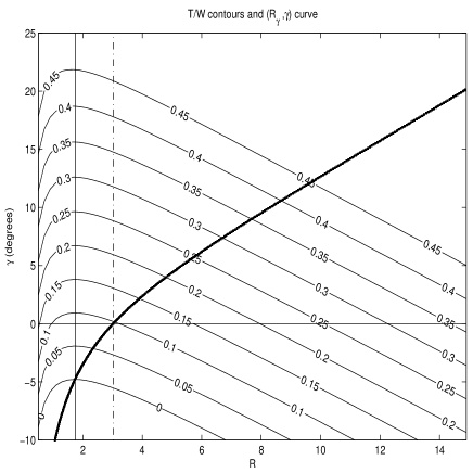
Figure 1: Contours of $T/W$ over $(\gamma,R)$, with the optimality curve $(\gamma,R_{\gamma})$

The angle $\gamma_{T/W}$ can be calculated explicitly, because the right-hand side of the equation

$${\frac{T}{W}}=C_{D_{0}}R_{\gamma}+\displaystyle{\frac{K\cos^{2}\gamma}{R_{\gamma}}}+\sin\gamma$$

is the function $\tau(\gamma)$ from (13) that can be inverted using MAPLE to yield

$$\sin(\gamma_{T/W})=\displaystyle{\frac{2(T/W)-\sqrt{(T/W)^{2}(1-12KC_{D_{0}})+64K^{2}C^{2}_{D_{0}}+16KC_{D_{0}}}}{2(1+4KC_{D_{0}})}}.$$ (14)

If inserted into (7), the positive root is infeasible. The above formula can be applied to calculate a Continuous Descent at nonzero idle thrust, or an optimal climb for a prescribed thrust policy as a function of altitude, using the ODE (9) inserting $\gamma_{T/W}$ and $R_{\gamma_{T/W}}$. We shall provide examples later.

If speed is prescribed, e.g. 250 knots indicated airspeed (KIAS) below 10000 ft, one has a prescribed $R$ and can use Figure 1 to read off a $\gamma_{R}$ such that $R_{\gamma_{R}}=R$. The only feasible solution is

$$6K\sin(\gamma_{R})=R-\sqrt{R^{2}+36K^{2}-12KC_{D_{0}}R^{2}},$$

and the thrust follows from (5) again. This will yield an optimal climb strategy under speed restriction, solvable again via (9). We shall come back to this in Section 6.

4 Variational Problem

So far, we have determined the maximal-range instantaneous speed assignment for an arbitrary flight plan $h(x)$, given via $R_{\gamma}$ or $V_{\gamma}$ of (12) or (13) for $\gamma=\arctan h^{\prime}(x)$. If this speed does not violate restrictions, it is the best one for that flight plan. But now we go a step further and vary the flight plans to find an optimal flight plan under all plans that allow the range-optimal instantaneous speed assignment.

To this end, we insert $R_{\gamma}$ into the right-hand side of (9) to get a variational problem for the flight path $h(x)$. The integrand for calculating $Z(x)=2\sqrt{W(x)}$ via

$$Z(x_{1})-Z(x_{0})=2\sqrt{W(x_{1})}-2\sqrt{W(x_{0})}=\int_{x_{0}}^{x_{1}}\displaystyle{\frac{dZ}{dx}}dx$$ (15)

is

$${\frac{dZ}{dx}}=-S\displaystyle{\frac{C(h)\sqrt{\rho(h)}}{\sqrt{2}}}\displaystyle{\frac{C_{D_{0}}R_{\gamma}+\displaystyle{\frac{K\cos^{2}\gamma}{R_{\gamma}}}+\sin\gamma}{\sqrt{R_{\gamma}}\cos\gamma}}=:F(h)G(h^{\prime}),$$ (16)

and the variational problem consists of finding $h(x)$ such that the integral in (15) is minimized. The integrand is a product of a function $F$ of $h$ and a function $G$ of $h^{\prime}$ via $\gamma=\arctan(h^{\prime})$. For such a variational problem, the Euler-Lagrange equation is

$$h^{\prime\prime}=\displaystyle{\frac{F^{\prime}(h)}{F(h)}}\left(\displaystyle{\frac{G(h^{\prime})}{G^{\prime\prime}(h^{\prime})}}-\displaystyle{\frac{G^{\prime}(h^{\prime})}{G^{\prime\prime}(h^{\prime})}}h^{\prime}\right)$$ (17)

by standard arguments of the Calculus of Variations, and we need the corresponding complicated derivatives of $F$ and $G$.

The function $G$ is dependent only on the drag polar, not on propulsion, and derivatives wrt. $h^{\prime}$ can be generated by symbolic computation, e.g. using MAPLE. The function $F(h)$ is $C(h)\sqrt{\rho(h)}$ up to constants and depends on propulsion only via the altitude-dependency of the specific fuel consumption $C(h)$. In simple models, e.g. [11] for turbofans and turbojets, $C(h)$ is an exponential function of $h$, as well as the air density $\rho(h)$. Then symbolic computation will work as well for the $h$-dependent part. Using the code generation feature of MAPLE, one gets ready-to-use expressions in MATLAB for solving the second-order ODE (17) for optimal flight plans $h(x)$, without any detour via Optimal Control.

A closer inspection of the Euler-Lagrange equation for the variational problem shows that $F^{\prime}(h)/F(h)$ is a constant if $C(h)$ and $\rho(h)$ have an exponential law, and then the right-hand-side of the Euler-Lagrange equation (17) is a pure equation in $h^{\prime}$. Since the equation is also autonomous, i.e. independent of $x$, the solutions $h(x)$ in the $(x,h)$ plane can be shifted right-left and up-down.

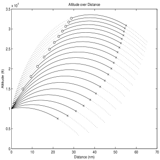
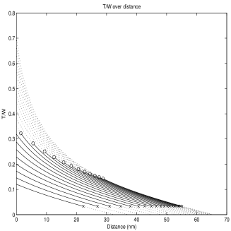
Figure 2: Some unconstrained flight paths for the SBJ model in [11], plots of $(h,x),\;(V,x),\;(T/W,x),\;(\gamma,h)$

Figure2 shows typical solutions of the Euler-Lagrange equation for the Standard Business Jet (SBJ) model from [11], starting at 10000 ft and ending at 3000 ft. A closer inspection of the differential equation reveals that the solutions are always concave in the $(x,h)$ plane, and the speed is always decreasing, see the two upper plots. The lower left plot shows the $T_{\gamma}/W$ values of (13), and these may be too large or too small to be admissible. Therefore all curves are dotted where the thrust restrictions are violated. The lower right plot of Figure 2 visualizes this in phase space, where we replaced $h^{\prime}$ by $\gamma=\arctan h^{\prime}$ for convenience. The trajectories there are traversed downwards, with decreasing $\gamma$, and the extremum of $h$ to the right.

This looks disappointing at first sight, but we have to take the thrust limits into account and view the variational problem as a constrained one. Such problems have the well-known property that solutions either follow the Euler-Lagrange equation or a boundary defined by the restrictions. In our case, only the solid curves between the circles and the crosses are solutions of the Euler-Lagrange equations that solve the unconstrained variational problem. When a solution of the variational problem hits a constraint, the Euler-Lagrange ODE is not valid anymore, but one can use the constraint to determine the solution. We shall do that in what follows, and point out that optimal full flight plans will follow the circles first, then depart from the circles to a solid line, and depart form the line at a cross to follow the crosses from that point on. This argument is qualitatively true, but needs a minor modification due to the fact that the true weight behaves slightly differently when we consider a single trajectory, while Figure 2 shows multiple trajectories.

5 Constrained Range-Optimal Trajectories

We now check the solutions of the variational problem when thrust restrictions are active. These are partial flight plans with range-optimal speed assignments as well as the partial flight plans that do not violate restrictions, being solutions of the Euler-Lagrange equation (17). To calculate the thrust-restricted parts, we assume thrust being given as a function of altitude, either as maximal admissible continuous thrust or as idle thrust. Inserting the current weight $W$, we use (14) to calculate the flight path angle $\gamma_{T/W}$ that yields the range-optimal $R_{\gamma_{T/W}}$ assignment via (12). Then an ODE system for $h$ and $W$ is set up using (8) and $h^{\prime}(x)=\tan\gamma_{T/W}$.

Doing this for maximal admissible continuous thrust yields range-optimal climb/cruise trajectories, while inserting idle thrust yields range-optimal Continuous Descent trajectories. Between these two parts of a range-optimal flight, there must be a transition from maximal admissible continuous thrust to idle thrust, and this transition must follow a solution of the Euler-Lagrange equation. In terms of Figure 2, the climb/cruise path reaches a circle, then follows one of the curves up to the cross marking idle thrust, and then a Continuous Descent trajectory follows. The Top of Descent point is reached in the transition part.

Starting at a given altitude and weight, the speed and the initial flight path angle are determined. Because the range-optimal speed $V_{\gamma}$ usually comes out to be well above 250 KIAS at low altitudes, we start our range-optimal trajectories at 10000 ft, and for the following plots we used a fixed starting weight at that altitude.

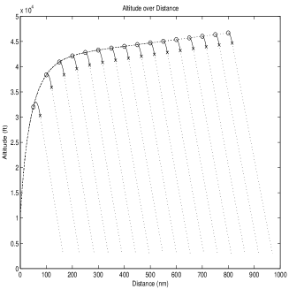
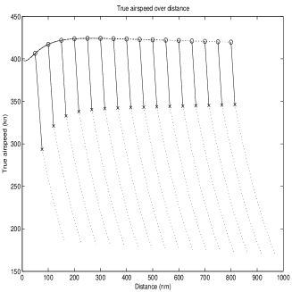
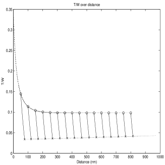
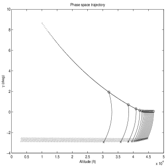
Figure 3: Some optimal three-piece flight paths for the SBJ model in [11], plots of $(h,x),\;(V,x),\;(T/W,x),\;(\gamma,h)$

Figure 3 shows range-optimal trajectories with the three parts described above, for the Small Business Jet of [11]. The climb/cruise part, using a maximal continuous thrust power setting of 0.98, is stopped at distances from 50 to 800 nm in steps of 50 nm to produce the different trajectories. When a transition is started, the final $\gamma$ of the climb is used to calculate an unconstrained solution of the Euler-Lagrange equation that performs a smooth transition to the Continuous Descent part at idle thrust. Along the Euler-Lagrange transition, the decreasing $T/W$ values are monitored, and the Continuous Descent is started when $T_{idle}/W$ is reached. The full range-optimal flight paths are in the top left plot, while the top right shows the true airspeed and the bottom left shows the $T/W$ values along the flight paths. The final plot is in phase space. One can compare with Figure 2, but there the total flight distances are much smaller. To arrive at a certain destination distance and altitude, the starting point of the transition has to be adjusted.

A close-up of one of the transitions is in Figure 4, namely the one where the transition is started at 400 nm. The transition takes about 15 nm, and the right-hand plot shows what the pilot should do for a range-optimal flight: decrease thrust from maximal continuous thrust to idle thrust slowly and roughly linearly, using about 15 nm. At high altitudes, the top-of-descent point is reached very shortly after the transition is started, see the phase space plot in Figure 3.

Figure 4: Transition part of an optimal three-piece flight path for the SBJ model in [11], plots of $(h,x),(T/W,x)$

This means that range-optimal long-distance flights above 10000 ft have necessarily three sections:

1. a climb/cruise at maximal continuous admissible thrust,

2. a transition following a solution of the Euler-Lagrange equation,

3. and a continuous descent at idle thrust.

Figure 3 shows that for high altitude the flight path angle tends to be constant. To analyze this effect, we go over to a single differential equation for $\gamma$ that has a stationary solution. We insert the prescribed thrust $T(h)$ into (13) to get

$${\frac{T(h)}{W}}=\tau(\gamma)=2\displaystyle{\frac{s^{2}+s\sqrt{s^{2}+12KC_{D_{0}}c^{2}}+4KC_{D_{0}}c^{2}}{s+\sqrt{s^{2}+12KC_{D_{0}}c^{2}}}}$$

with $\tau$ from (13) being the inverse function of (14) in terms of $s=\sin\gamma$ and $c=\cos\gamma$. The idea now is to get rid of $W$ by taking $h$-derivatives and

$$\begin{array}[]{rcl}T^{\prime}(h)&=&\displaystyle{\frac{d}{dh}}(W\tau(\gamma))=\displaystyle{\frac{dW}{dh}}\tau(\gamma)+\displaystyle{\frac{T(h)}{\tau(\gamma)}}\tau^{\prime}(\gamma)\displaystyle{\frac{d\gamma}{dh}},\\[8.5359pt] V^{2}&=&\displaystyle{\frac{2R(\gamma)W}{\rho(h)S}}=\displaystyle{\frac{2R(\gamma)T(h)}{\tau(\gamma)\rho(h)S}}\\[8.5359pt] \displaystyle{\frac{dW}{dh}}&=&\displaystyle{\frac{\dot{W}}{\dot{h}}}=\displaystyle{\frac{-C(h)T(h)}{V\sin\gamma}}=-\displaystyle{\frac{C(h)\sqrt{T(h)\tau(\gamma)\rho(h)S}}{\sin\gamma\sqrt{2R(\gamma)}}}\end{array}$$

to arrive at the single differential equation

$${\frac{T^{\prime}(h)}{T(h)}}=-\displaystyle{\frac{C(h)\sqrt{\rho(h)}}{\sqrt{T(h)}}}\displaystyle{\frac{\tau^{3/2}(\gamma)}{\sin\gamma\sqrt{R(\gamma)}}}\displaystyle{\frac{\sqrt{S}}{\sqrt{2}}}+\displaystyle{\frac{\tau^{\prime}(\gamma)}{\tau(\gamma)}}\displaystyle{\frac{d\gamma}{dh}}\\$$

governing range-optimal climb/cruise at prescribed thrust. If a constant $\gamma$ would solve this ODE, the equation

$${\frac{-T^{\prime}(h)}{\sqrt{T(h)}C(h)\sqrt{\rho(h)}}}=\displaystyle{\frac{\tau^{3/2}(\gamma)}{\sin\gamma\sqrt{R(\gamma)}}}\displaystyle{\frac{\sqrt{S}}{\sqrt{2}}}$$

must hold over a certain range of $h$. But for the turbojet/turbofan propulsion models of [11] and the exponential air density model (3), all parts of the left-hand side are certain powers of $\rho(h)$ that finally cancel out, letting the left-hand side be a constant that only depends on the power setting. The right-hand side has a singularity for $\gamma=0$, and there always is a small fixed positive angle $\gamma$ solving the above equation. The ODE solution tends to this for increasing $h$, explaining the constant final climb angle in Figure 3 for prescribed thrust. The left-hand side seems to be a crucial parameter for propulsion design, relating consumption to thrust and altitude for both turbojets and turbofans.

6 Prescribed Speed

To deal with the usual speed restriction below 10000 ft, we have to abandon the above scenario, because we cannot minimize fuel consumption with respect to speed anymore. If the speed is given (in terms of $R$), equation (5) still has one degree of freedom, connecting $T/W$ to the flight path angle $\gamma$, and we have to solve for a range-optimal climb strategy in a different way now, going directly to a variational problem.

Implementing a 250 KIAS restriction including conversion to true airspeed, we have an altitude-dependent prescribed speed $V_{F}(h)$. Since air density $\rho$ is also $h$-dependent, so is the dynamic pressure $\bar{q}(h)=\frac{1}{2}\rho(h)V_{F}(h)^{2}$ and the variable $U(h)=\bar{q}(h)S$ connecting the pressure ratio $R$ to the weight $W$ via

$$R(h,W)=\displaystyle{\frac{\bar{q}(h)}{\frac{W}{S}}}=\displaystyle{\frac{\rho(h)V_{F}^{2}(h)S}{2W}}=\displaystyle{\frac{U(h)}{W}}.$$

Then (5) yields

$$\begin{array}[]{rcl}T=C_{D_{0}}U(h)+\displaystyle{\frac{KW^{2}\cos^{2}\gamma}{U(h)}}+W\sin\gamma.\end{array}$$

Inserting into the fuel consumption integrand, we get

$$\begin{array}[]{rcl}-{W^{\prime}(x)}&=&\displaystyle{\frac{C(h)}{V_{F}(h)}}\left(\displaystyle{\frac{C_{D_{0}}U(h)}{\cos\gamma}}+\displaystyle{\frac{KW^{2}\cos\gamma}{U(h)}}+W\tan\gamma\right)\\[11.38092pt] \end{array}$$

which is a Lagrangian $L(W,h,h^{\prime})=L(W,u,v)$ and leads to a variational problem with an Euler-Lagrange equation. In contrast to Section 4, the weight is not eliminated, but we simply keep it in the Lagrangian. We only need the Lagrangian for $h$ up to 10000 ft, and then we can fit each $h$-dependent part with good accuracy by a low-degree polynomial in $h$.The $\gamma$- or $h^{\prime}=\tan\gamma$- dependent parts can be differentiated symbolically, as well as the polynomial approximations to the $h$-dependent parts. We get the ODE system

$$\begin{array}[]{rcl}h^{\prime}&=&v\\ v^{\prime}&=&\displaystyle{\frac{1}{L_{vv}(W,u,v)}}(L_{u}(W,u,v)-L_{vu}(W,u,v)v)\\ W^{\prime}&=&-L(W,u,v)\end{array}$$

for the Euler-Lagrange flight paths, under suitable initial or boundary value conditions, and we can roughly repeat Section 4 for the new variational problem. Above, the subscripts denote the partial derivatives.

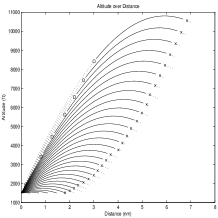
Figure 5: Unconstrained range-optimal solutions at 250 KIAS, flight path, $T/W$ ratio, and phase space

For the aircraft model in [11] started at 1500 ft with maximal weight, we get Figure 5 showing range-optimal unconstrained trajectories for flight at 250 KIAS at low altitudes. Like in the previous figures, the dotted parts violate thrust restrictions. For a long-range flight, the trajectory reaching $\gamma=0$ exactly at 10000 ft should be selected, and but it needs excessive thrust at the beginning.

Therefore the upper thrust limit for the variational problem has to be accounted for, and range-optimal trajectories for a 250 KIAS climb will consist of two pieces: the first with maximal admissible thrust, and the second as a transition satisfying the Euler-Lagrange equation for the optimal speed-restricted case. Because the range-optimal trajectories over 10000 ft require higher airspeed, the second piece should reach horizontal flight at 10000 ft in order to be followed by an acceleration at 10000 ft.

The climb at maximal admissible continuous thrust $T_{max}(h)$ and prescribed airspeed $V_{F}(h)$ is completely determined by the initial conditions, and (5) is solved for $\gamma$ via

$$2K\sin\gamma=R-\sqrt{R^{2}-4KRT/W+4KC_{D_{0}}R^{2}+4K^{2}}$$

to get the flight path.

Figure 6 shows such two-piece climbs at 250 KIAS, starting at 1500 ft and stopping the first part at distance 1 to 4 nm in steps of 0.5. The second part has an optiomally reduced thrust and is stopped at $\gamma=0$. For long-range flights, the trajectory ending at 10000 ft should be selected.

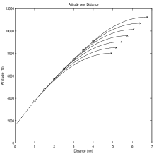
Figure 6: Two-piece range-optimal solutions at 250 KIAS, flight path, $T/W$ ratio, and phase space

But these trajectories need 250 KIAS to be started, and this calls for an acceleration at the “acceleration” altitude where clean configuration is reached and “at which the aircraft accelerates towards the initial climb speed” [1, p. 1245]. Another acceleration will be necessary at 10000 ft, because the range-optimal climb below 10000 ft is flown at 250 KIAS, while the range-optimal climb to higher altitudes starts at roughly 400 kts, see Figure 3, top right. But if flown at high thrust, these two accelerations can be neglected for long-range flights. They take 1 nm and 6 nm, respectively, for the model aircraft of [11].

7 Flight Level Change in Cruise

We now consider the practical situation that a long-distance high-altitude cruise under Air Traffic Control is a sequence of level flights with various short-term flight-level changes. These are short-term changes of $\gamma$, and it is debatable whether they should be considered as quasi-steady flight. We know now that such a flight is never range-optimal, but each level section should apply the $V_{0}$ speed given by (11). This means that all level flight sections in cruise use the same $R_{0}$ from (10), leading to the same $T/W$ ratio via (5), no matter what the flight level or the propulsion model is. Only the drag polar is relevant. Again, it turns out to be convenient to work in terms of $R$ to be independent of weight and altitude.

The $V_{0}$ speed at $\gamma=0$ then is a function of weight and altitude alone, and flight level changes should comply with this, i.e. the speed should still vary smoothly, while $\gamma$ and thrust may change rapidly. We shall deal with this by keeping the flight level change as quasi-steady flight, except for the beginning and the end, where we allow an instantaneous and simultaneous change of $\gamma$ and thrust that compensate each other.

The idea is to keep the quasi-steady flight equation (5) and the $R_{0}$ equation (10) valid at all times. Then a jump in $\gamma$ must be counteracted by a jump in thrust, one in the beginning and one in the end of the flight level change. These instants are not quasi-steady, but the rest is.

Consider a climb from altitude $h_{0}$ to altitude $h_{1}$. When flying at $V_{0}$ at $h_{0}$ at maximal thrust $T_{max}(h_{0})$, the flight level change is impossible. Otherwise, the quasi-steady flight equation (5) at time $t_{0}$ and $\gamma=0$ is

$${\frac{T_{0}}{W_{0}}}=C_{D_{0}}R_{0}+\displaystyle{\frac{K}{R_{0}}},\;T_{0}<T_{max}(h_{0}),$$ (18)

and we apply maximal thrust and go over to

$${\frac{T_{max}(h_{0})}{W_{0}}}=C_{D_{0}}R_{0}+\displaystyle{\frac{K}{R_{0}}}\cos^{2}\gamma_{0}+\sin\gamma_{0}$$

defining a unique climb angle $\gamma_{0}$ satisfying

$$2K\sin\gamma_{0}=R_{0}-\sqrt{R_{0}^{2}-4K\displaystyle{\frac{T_{max}(h_{0})}{W_{0}}}R_{0}+4KC_{D_{0}}R_{0}^{2}+4K^{2}}.$$ (19)

We could keep this angle for the climb, but we might reach the thrust limit if we do so. Therefore we prefer to satisfy

$${\frac{T_{max}(h)}{W(h)}}=C_{D_{0}}R_{0}+\displaystyle{\frac{K}{R_{0}}}\cos^{2}\gamma(h)+\sin\gamma(h)$$

at each altitude using

$$K\sin\gamma(h)=R_{0}-\sqrt{R_{0}^{2}-4K\displaystyle{\frac{T_{max}(h)}{W(h)}}R_{0}+4KC_{D_{0}}R_{0}^{2}+4K^{2}}.$$

This is put into an ODE system for $h$ and $W$ with $\gamma$ as an intermediate variable, namely

$$\begin{array}[]{rcl}h^{\prime}&=&\tan\gamma(h)\\ W^{\prime}&=&-\displaystyle{\frac{C(h)T_{max}(h)}{V_{0}(h,W)\cos\gamma(h)}}.\end{array}$$

The result is a climb with constant $R_{0}$ that keeps $V_{0}$ of (11) at all times and thus starts and ends with the correct speed for range-optimal level flight. For descent, the same procedure is used, but idle thrust is inserted. If the altitude change is small, the solution is close to using the fixed climb/descent angle $\gamma_{0}$ of (19). At the end of the flight-level change at altitude $h_{1}$, the final speed $V_{0}(h_{1},W_{1})$ is the starting speed of the next level flight, and the thrust has to be decreased instantaneously to $T_{1}$ in order to keep the ratio

$${\frac{T_{0}}{W_{0}}}=\displaystyle{\frac{T_{1}}{W_{1}}}$$

from (18).

We omit plots for our standard aircraft model, because they all show that the crude simplification

$${\frac{h_{1}-h_{0}}{x_{1}-x_{0}}}\approx\gamma_{0}\approx\displaystyle{\frac{T-T_{0}}{W_{0}}}$$

holds for small altitude changes between level flights, where the thrust $T$ is either $T_{max}$ or $T_{idle}$. Thus in $(x,h)$ space the transition is very close to linear with the roughly constant climb angle given above.

But we have to ask whether climbing at maximal thrust is fuel-to-distance optimal against all other choices of thrust. If we insert the above approximation into the fuel consumption with respect to the distance and just keep the thrust varying, we get

$$\int_{x_{0}}^{x_{1}}\displaystyle{\frac{CT}{V\cos\gamma}}dx\approx W_{0}(h_{1}-h_{0})+T_{0}(x_{1}-x_{0})$$

up to a factor, and thus we should minimize the climb angle if we relate consumption to distance. For descent, this leads to taking $T_{idle}$ and is easy to obey, but for climb the range-optimal solutions cannot be taken because they take too long. Consequently, pilots are advised to perform the climb at smallest rate allowed by ATC.

8 Flight Phases for Maximal Range

As long as Air Traffic Control does not interfere, we now see that a long range-optimal flight should have the following phases:

1. Takeoff to clean configuration and acceleration altitude,

2. accelerate there to 250 KIAS at maximal admissible continuous thrust,

3. climb at maximal admissible continuous thrust, keeping 250 KIAS and following the range-optimal angle selection strategy of Section 6, and continuing with

4. a solution of the variational problem given there to end at precisely 10000 ft in horizontal flight,

5. accelerate at 10000 ft in horizontal flight until the required speed for a range-optimal climb is reached,

6. perform a range-optimal climb/cruise following Sections 4 and 3 at maximal continuous admissible thrust until shortly before the top-of-descent point, leaving that climb for

7. an Euler-Lagrange path satisfying the variational problem of Section 4 until thrust is idle,

8. do a continuous descent at idle thrust down to the Final Approach Fix.

To arrive at the right distance and altitude, the time for starting phase 7 needs to be be varied, like in Figure 3.

If ATC requires horizontal flight phases and correspondent flight-level changes, step 6 is followed by

• an Euler-Lagrange path satisfying the variational problem of Section 4 to reach the prescribed altitude,

• using Section 3 for range-optimal speed at level flight, and

• flight path changes following Section 7,

but the flight will not be range-optimal. Various examples show that a continuous descent from high altitude ends up at speeds below 250 KIAS at 10000 ft, and deceleration is not needed.

Flight paths for shorter distances should follow the above steps for long-haul flights up to a certain point where they take a “shortcut” from the long-distance flight pattern.

9 Conclusion

Except for the two accelerations at 10000 ft and “acceleration altitude”, this paper provided range-optimal flight paths as simple solutions of certain ordinary differential equations, without using Control Theory or other sophisticated tools. However, everything was focused on quasi-steady flight within simple atmosphere and propulsion models. Also, the numerical examples were currently confined to the Small Business Jet of [11] with its turbojet engines. However, most of the results are general enough to be easy to adapt for other aircraft and engine characteristics, and this is left open.

References

- [1] Airbus. Airbus A 380 Flight Crew Operating Manual. Airbus S.A.S Customer Services Directorate, 31707 Blagnac, France, 2011. Reference: KAL A 380 Fleet FCOM, Issue Date: 03 Nov. 2011.
- [2] J.T. Betts. Survey of numerical methods for trajectory optimization. Journal of Guidance, Control, and Dynamics, 21:193–207, 1998.
- [3] A.E. Bryson, M.N. Desai Jr., and W.C. Hoffman. Energy-state approximation in performance optimization of supersonic aircraft. Journal of Aircraft, 6:481–488, 1969.
- [4] J.W. Burrows. Fuel optimal trajectory computation. Journal of Aircraft, 19:324–329, 1982.
- [5] A.J. Calise. Extended energy management methods for flight performance optimization. AIAA Journal, 15:314–321, 1977.
- [6] A. Franco and D. Rivas. Analysis of optimal aircraft cruise with fixed arrival time including wind effects. Aerospace Science and Technology, 32:212–222, 2014.
- [7] A. Franco, D. Rivas, and A. Valenzuela. Minimum-fuel cruise at constant altitude with fixed arrival time. Journal of Guidance, Control, and Dynamics, 33:280–285, 2010.
- [8] J. García-Heras, M. Soler, and F.J. Sáez. Collocation methods to minimum-fuel trajectory problems with required time of arrival in ATM. Journal of Aerospace Information Systems, 13:243–265, 2016.
- [9] A. Gardi, R. Sabatini, and S. Ramasamy. Multi-objective optimisation of aircraft flight trajectories in the ATM and avionics context. Progress in Aerospace Sciences, 83:1–36, 2016.
- [10] G. Huang, Y. Lu, and Y. Nan. A survey of numerical algorithms for trajectory optimization of flight vehicles. Sci. China Technol. Sci., 55:2538–2560, 2012.
- [11] D.G. Hull. Fundamentals of Airplane Flight Mechanics. Springer, 2007.
- [12] W. Maazoun. Conception et analyse d’un système d’optimisation de plans de vol pour les avions. PhD thesis, École Polytechnique de Montréal, 2015.
- [13] A. Miele. Flight Mechanics: Theory of Flight Paths. Dover Books on Aeronautical Engineering, reprint of the 1962 original, 2016.
- [14] R. Myose, T. Young, and G. Sim. Comparison of business jet performance using different strategies for flight at constant altitude. AIAA 5th ATIO and 16th Lighter-Than-Air Sys Tech. and Balloon Systems Conferences, 2005.
- [15] S.G. Park and J.-P. Clarke. Optimal control based vertical trajectory determination for continuous descent arrival procedures. Journal of Aircraft, 52:1469–1480, 2015.
- [16] D.H. Peckham. Range Performance in Cruising Flight. National Technical Information Service, 1974.
- [17] W. F. Phillips. Mechanics of Flight. John Wiley & Sons, 2010. Second Edition.
- [18] B.L. Pierson and S.Y. Ong. Minimum-fuel aircraft transition trajectories. Mathematical and Computer Modelling, 12:925–934, 1989.
- [19] J.E. Rader and D.G. Hull. Computation of optimal aircraft trajectories using parameter optimization methods. Journal of Aircraft, 12:864–866, 1975.
- [20] E.S. Rutowski. Energy approach to the general aircraft performance problem. Journal of the Aeronautical Sciences, 21:187–195, 1954.
- [21] A. Saucier, W. Maazoun, and F. Soumis. Optimal speed-profile determination for aircraft trajectories. Aerospace Science and Technology, 2017. In Press.
- [22] R.F. Stengel. Flight Dynamics. Princeton University Press, 2004.
- [23] A. Valenzuela and D. Rivas. Optimization of aircraft cruise procedures using discrete trajectory patterns. Journal of Aircraft, 51:1632–1640, 2014.
- [24] N.X. Vinh. Optimal Trajectories in Atmospheric Flight. Elsevier, reprint in 2012, 1980.
- [25] N.X. Vinh. Flight Mechanics of High-Performance Aircraft. Cambridge University Press, 1995.
- [26] K.S. Yajnik. Energy-turn-rate characteristics and turn performance of an aircraft. Journal of Aircraft, 14:428–433, 1977.