Supplementary Material for Observing Power-Law Dynamics of Position-Velocity Correlation in Anomalous Diffusion

Gadi Afek, Jonathan Coslovsky, Arnaud Courvoisier, Oz Livneh and Nir Davidson

Department of Physics of Complex Systems, Weizmann Institute of Science, Rehovot 76100, Israel

Phase-space tomography and experimental sequence

The experimental sequence, depicted in figure 1 is as follows: A cloud of $\sim 10^{5}$ ⁸⁷Rb atoms are loaded into a crossed dipole trap from a Raman-sideband cooled, polarization gradient cooled MOT. After a short evaporation and equilibration phase the atoms are loaded adiabatically into a single-beam dipole trap providing confinement in the radial axis. A lattice pulse is applied with a selected lattice depth $U_{0}$ for a specific exposure time $t$. The detection phase is comprised of a counter-propagating Raman velocity-selective $\pi$-pulse given at a specific two-photon detuning, selecting a narrow velocity class and transferring the atoms contained in it to the upper ground-state level [1] (fig. 2). These atoms are then imaged using state-selective absorption imaging.

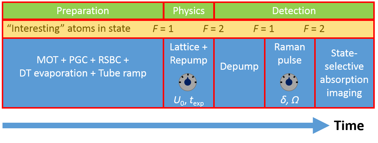
Figure 1: Scheme of the experimental sequence. ⁸⁷Rb atoms are prepared in a crossed dipole trap and then loaded into a 1D ”tube trap”. Then a time-varied and depth-varied lattice pulse is given, followed be the detection stage comprised of a Raman velocity-selective pulse followed by absorption imaging.

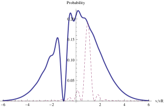
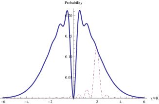
Figure 2: Analytic calculation of the distribution of momentum in $\left|1\right>$ and $\left|2\right>$ states (solid and dashed lines, respectively) after a $\pi$ pulse for two different ”digging points” (left and right). Notice that a net momentum of twice the one-photon recoil momentum is imparted to the state $\left|2\right>$ in completing the hyperfine transition. The location of the ”digging point” is a function of the detuning $\delta$. Detection of the transferred population can be deconvolved back to give the original (unknown) distribution

An example of the phase-space images obtained can be seen in figure 3. The shearing of the phase-space in the ballistic case ($U_{0}=0$) is clearly visible, as is the fact that correlations are suppressed for stronger lattices.

Figure 3: Selected raw data images, for three lattice powers (rows) and three exposure times (columns). Position is on the vertical axis and velocity on the horizontal axis. The buildup of correlations in the ballistic ($U_{0}=0$) regime is clearly visible, as is the suppression of correlations in the regime where $U_{0}>0$.

Extraction of the correlation

To quantitatively analyze the position-velocity correlations we use the definition

$$C_{xv}(t)\equiv\frac{\left<\delta\vec{x}(t)\cdot\delta\vec{v}(t)\right>}{\sqrt{\left<\delta\vec{x}^{2}(t)\right>\left<\delta\vec{v}^{2}(t)\right>}},$$ (1)

where $\left<...\right>$ denotes the ensemble average and $\delta\vec{x}=\vec{x}-\left<\vec{x}\right>$. The normalization bounds the correlation between 1 and -1. If the PSD distribution is known, one can replace the ensemble average with a sum over the PSD. We extract the information about the correlations in two different ways:

1. direct calculation from the raw data, thresholded by 10% of the maximal pixel (all pixels with values $<10\%$ of the maximal pixel are set to zero)

2. extracting the asymmetry parameter from the data by finding the center using fits on the one-axis-integrated data and dividing into quadrants.

The asymmetry method works by extracting an asymmetry parameter from the data by finding the center using fits on the one-axis-integrated data, dividing into quadrants, summing the pixels in each of the quadrants to obtain $Q_{i}$ and extracting $AS=\frac{Q_{2}+Q_{4}-Q_{1}-Q_{3}}{Q_{\text{tot}}}$. It is then transformed into correlation using an analytic calibration, in which a bivariate normal distribution with a given correlation is integrated from $-\infty$ to zero and from zero to $\infty$ to generate the $Q_{i}$’s, and obtain:

$$AS=-1+\frac{8\arccos(C)}{5\pi-2\arcsin(C)-2\arctan(\sqrt{1/C^{2}-1})}$$ (2)

which is then inverted numerically and used for the transformation between $AS$ and $C$. An example of the division into quadrants is shown in fig. 4, along with the calibration curve.

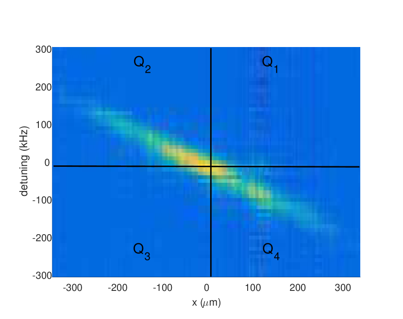
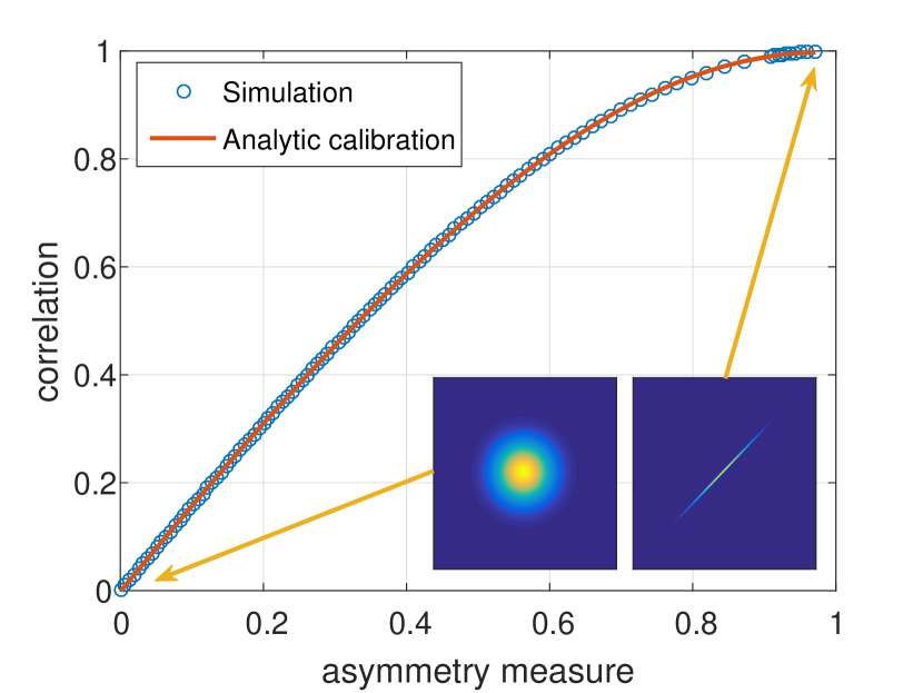
Figure 4: (left) High resolution (low Rabi frequency, 30 averages per slice) phase-space image with division into quadrants. Here the vertical axis is the two-photon detuning of the Raman beams. The asymmetry measure is defined as $AS=\frac{Q_{2}+Q_{4}-Q_{1}-Q_{3}}{Q_{\text{tot}}}$. (right) The calibration curve of the correlation as a function of the asymmetry measure. Insets show the simulated PSDD for $C=0$ and $C=99.9\%$.

The correlations extracted using these methods are shown in fig. 5 (top panels). One can see that the two sets behave similarly but the asymmetry one suffers less from noise. For further verification we compare the correlations extracted using the two methods on phase-spaces obtained from the two different types of simulations described in the main text. In the bottom panel of fig. 5 the real correlation is plotted against that obtained from the asymmetry method. The agreement is good, especially considering that the phase spaces in question are highly non-Gaussian.

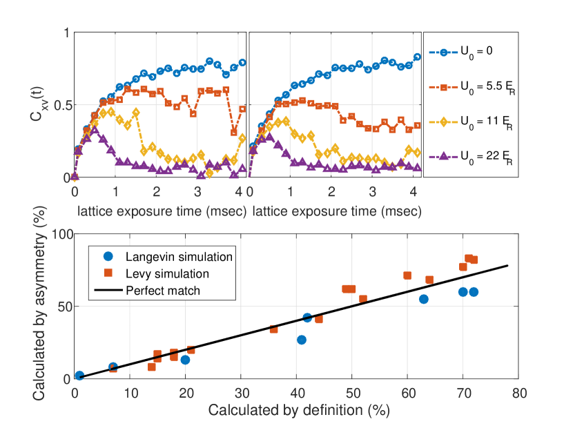
Figure 5: Position-velocity correlations, directly calculated using the definition 1 (top left) and by using the asymmetry method (top right). Here the threshold is 10% (meaning pixels that have an intensity $<10\%$ of the maximal pixel are set to zero). Comparing the correlations calculated using both methods on phase spaces obtained by the simulation (bottom), we obtain good agreement, especially considering that the phase spaces in question are highly non-Gaussian.

Broadening

a broadening effect arising from a finite two-photon Rabi frequency required to transfer enough atoms per velocity class in order to obtain reasonable SNR. The broadened correlation is a function of the ratio between the width of the Raman $\pi$-pulse  (i.e., the Rabi frequency) and the standard deviation of the velocity distribution: $C_{xv}/C_{xv}^{0}=1/\sqrt{1+(\sigma_{\Omega}/\sigma_{v})^{2}}$, where $C_{xv}$ is the broadened (measured) correlation, $C_{xv}^{0}$ is the original correlation, $\sigma_{\Omega}$ is the width of the Rabi $\pi$-pulse in units of velocity and $\sigma_{v}$ is the width of the velocity distribution. This allows for a rescaling of the correlation data to account for the Rabi broadening such that the ballistic correlations saturate at unity 6. The calculation is performed by convolving a bivariate normal distribution $f(x,v,C)$ with a ”Rabi” pulse $\frac{1}{\sqrt{2\pi\sigma_{\Omega}^{2}}}\exp(-v^{2}/2\sigma_{\Omega}^{2})$, and then calculating the ”measured” correlation using the definition given in eq. 1.

Figure 6: Position-velocity correlations in ballistic expansion. The solid line is a fit to the analytic expression given in the paper, with the additional fitting parameter $C_{\infty}$ needed to account for broadening due to the finite two-photon Rabi frequency. As the Rabi frequency is reduced the broadening is less apparent, in the expense of SNR. The left (right) phase-space reconstruction corresponds to the light blue (green) data.

Fitted parameters for the interpolation function

For the fit to the data depicted in figure 2 of the main text, we use the generalized interpolation function given in equation 9 of the main text. Figure 7 shows the fitted parameters $\omega_{\text{osc}}$ and $\Gamma$, shown in full symbols, along with their errors for both the unexcluded fit of fig. 2 (a) and the excluded fit of fig. 2(b) of the main text. The parameters are compared to those obtained independently (empty symbols) by either a trap oscillations experiment (giving a small kick to the trapped atoms, and imaging the oscillations in the trap) in the case of $\omega_{\text{osc}}$ or an exponential fit to the velocity dynamics in the case of $\Gamma$.

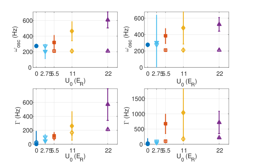
Figure 7: fitted parameters $\omega_{\text{osc}}$ (top) and $\Gamma$ (bottom), shown in full symbols, along with their errors for both the unexcluded fit of fig. 2 (a) (left) and the excluded fit of fig. 2(b) (right) of the main text. The parameters are compared to those obtained independently (empty symbols) by either a trap oscillations experiment or an exponential fit to the velocity dynamics.

Full derivation of the normal-diffusion limit

We calculate the position-velocity cross-correlation coefficient according to 1 for the case of simple Brownian motion. Beginning with the Langevin equation describing the instantaneous acceleration of a particle in a medium [2, 3],

$$\dot{\vec{v}}=-\Gamma\vec{v}+\vec{\mathcal{A}}$$ (3)

where $\vec{v}$ is the velocity vector, $\Gamma$ is the drag coefficient setting the timescale for transition between the ballistic and diffusive regimes and $\vec{\mathcal{A}}$ is the Langevin random acceleration. For the sake of simplicity of notations we assume from here on $\left<x\right>=\left<v\right>=0$, hence $\delta x=x$ and $\delta v=v$. The numerator of eq. 1 can be calculated by noticing that-

$$\frac{d}{dt}\left<\vec{x}\cdot\vec{v}\right> =\left<\frac{d}{dt}(\vec{x}\cdot\vec{v})\right>=\left<\vec{x}\cdot\frac{d\vec{v}}{dt}+\vec{v}\cdot\frac{d\vec{x}}{dt}\right>$$ (4)

$$=\left<\vec{x}\cdot(-\Gamma\vec{v}+\vec{\mathcal{A}})+\vec{v}^{2}\right>$$

$$=-\Gamma\left<\vec{x}\cdot\vec{v}\right>+\left<\vec{v}^{2}\right>$$

Between the 2nd and 3rd line we use the fact that due to the randomness of the Langevin acceleration $\left<\vec{x}\cdot\vec{\mathcal{A}}\right>=0$. The time dependence of $\left<\vec{v}^{2}\right>$ is given by-

$$\left<\vec{v}^{2}\right>=v_{0}^{2}+(v_{eq}^{2}-v_{0}^{2})(1-e^{-2\Gamma t})$$ (5)

with $v_{0}^{2}=\sigma_{v}^{2}(t=0)$, the initial variance of the velocity distribution, and $v_{eq}^{2}=\sigma_{v}^{2}(t\to\infty)=\frac{3k_{B}T}{m}$ according to equipartition in 3D ($k_{B}$ is the Boltzmann constant, $T$ is the temperature and $m$ the mass of the particle). Substituting into eq. 4 and solving under an uncorrelated initial condition $\left<\vec{x}(t)\cdot\vec{v}(t)\right>|_{t=0}=0$ we get:

$$\left<\vec{x(t)}\cdot\vec{v(t)}\right>=\frac{e^{-2\Gamma t}\left(e^{\Gamma t}-1\right)\left(v_{eq}^{2}\left(e^{\Gamma t}-1\right)+v_{0}^{2}\right)}{\Gamma}$$ (6)

Next we require the terms in the denominator of 1. The velocity was already presented in 5 and we just need to take its square root. The position, however, requires the solution of the differential equation-

$$\frac{d^{2}\left<\vec{x}^{2}\right>}{dt^{2}}+\Gamma\frac{d\left<\vec{x}^{2}\right>}{dt}=2v_{0}^{2}e^{-2\Gamma t}+2v_{eq}^{2}(1-e^{-2\Gamma t})$$ (7)

under the initial conditions $\left<\vec{x}^{2}(0)\right>=x_{0}^{2}$ and $\frac{d\left<\vec{x}^{2}\right>}{dt}|_{t=0}=0$. This gives:

$$\left<\vec{x}^{2}\right>=\frac{e^{-2\Gamma t}\left(v_{0}^{2}\left(e^{\Gamma t}-1\right)^{2}+v_{eq}^{2}\left(e^{2\Gamma t}(2\Gamma t-3)+4e^{\Gamma t}-1\right)+\Gamma^{2}x_{0}^{2}e^{2\Gamma t}\right)}{\Gamma^{2}}$$ (8)

Now we switch to the following unitless parameters:

• $\eta\equiv\frac{v_{0}^{2}}{v_{eq}^{2}}$ denoting the deviation of the initial velocity distribution width from its equilibrium value (set to unity in the main text for simplicity).

• $\omega_{osc}\equiv\sigma_{v}(0)/\sigma_{x}(0)$, the previously defined trap oscillation frequency that sets, under thermal equilibrium, the ratio of the initial conditions of the velocity and the position.

and combine everything to get the main result:

$$\frac{\left(e^{\Gamma t}-1\right)\left(\eta+e^{\Gamma t}-1\right)}{\sqrt{\left(\eta+e^{2\Gamma t}-1\right)\left[(\eta-1)+e^{2\Gamma t}\left(\eta\left(\frac{\Gamma}{\omega}\right)^{2}+(\eta+2\Gamma t-3)\right)-2(\eta-2)e^{\Gamma t}\right]}}$$ (9)

Setting $\eta=1$ we reobtain eq. 8 of the paper:

$$C_{xv}(t)=\frac{e^{-\Gamma t/2}\left(e^{\Gamma t}-1\right)}{\left[2+e^{\Gamma t}\left((\Gamma/\omega_{\text{osc}})^{2}+2\Gamma t-2\right)\right]^{1/2}}$$ (10)

Analyzing the timescales inherent to the system yields the following insight: There exist two time scales and two temporal scalings. The buildup scales linearly in time and saturates at unity with a timescale of $1/\omega_{\text{osc}}$. The decay scales like $t^{\gamma}$ with a timescale of $1/\Gamma$. The transition between the buildup and decay occurs at a timescale $\tau_{m}$, which is approximately the average $\left(1/\omega_{\text{osc}}+1/\Gamma\right)/2$. It is henceforth evident that observing the short-time correlation dynamics requires $\tau_{m}$ to be within the measurement time. To be more precise, maximization of eq. 10 yields the following transcendental equation for $\tau_{m}$, the maximal correlation time:

$$\Gamma\left(\Gamma+2\tau_{m}\omega_{\text{osc}}^{2}\right)-2\omega_{\text{osc}}^{2}\sinh(\Gamma\tau_{m})=0$$ (11)

that can be solved numerically to give the exact time and value of the maximal correlation in this model. In fig. 8, we plot eq. 10 as a function of time for different values of $\omega_{\text{osc}}$ and $\Gamma$. The light blue circles indicate the maximum calculated by eq. 11 and the dashed black lines are the approximation obtained by taking the average of the two timescales $\left(1/\omega_{\text{osc}}+1/\Gamma\right)/2$, showing that it is a valid approximation. These insights hold also for the case of anomalous diffusion, where the only difference with respect to this analysis is the scaling of $t^{\gamma}$ instead of the specific $t^{-1/2}$.

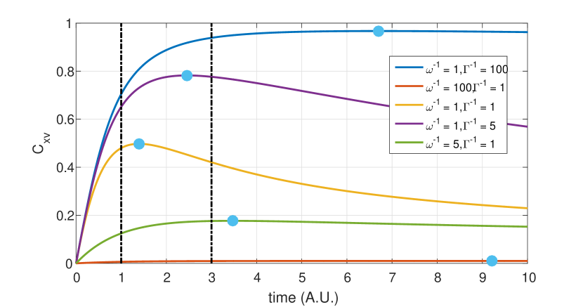
Figure 8: Analytic plot of eq. 10 as a function of time for different values of $\omega_{\text{osc}}$ and $\Gamma$. The light blue circles indicate the maximum calculated by eq. 11 and the dashed black lines are the approximation obtained by taking the average of the two timescales $\left(1/\omega_{\text{osc}}+1/\Gamma\right)/2$.

References

- Moler et al. [1992] K. Moler, D. S. Weiss, M. Kasevich, and S. Chu, Physical Review A 45, 342 (1992).
- Pathria [2006] R. Pathria, Statistical mechanics (Butterworth Heinemann, Oxford, UK, 2006).
- Gillespie and Seitaridou [2012] D. T. Gillespie and E. Seitaridou, Simple Brownian diffusion: an introduction to the standard theoretical models (Oxford University Press, 2012).