From quantum stochastic differential equations to Gisin-Percival state diffusion

Abstract

Starting from the quantum stochastic differential equations of Hudson and Parthasarathy (Comm. Math. Phys. 93, 301 (1984)) and exploiting the Wiener-Itô-Segal isomorphism between the Boson Fock reservoir space $\Gamma(L^{2}(\mathbb{R}_{+})\otimes(\mathbb{C}^{n}\oplus\mathbb{C}^{n}))$ and the Hilbert space $L^{2}(\mu)$, where $\mu$ is the Wiener probability measure of a complex $n$-dimensional vector-valued standard Brownian motion $\{\mathbf{B}(t),t\geq 0\}$, we derive a non-linear stochastic Schrödinger equation describing a classical diffusion of states of a quantum system, driven by the Brownian motion $\mathbf{B}$. Changing this Brownian motion by an appropriate Girsanov transformation, we arrive at the Gisin-Percival state diffusion equation (J. Phys. A 167, 315 (1992)). This approach also yields an explicit solution of the Gisin-Percival equation, in terms of the Hudson-Parthasarathy unitary process and a radomized Weyl displacement process. Irreversible dynamics of system density operators described by the well-known Gorini-Kossakowski-Sudarshan-Lindblad master equation is unraveled by coarse-graining over the Gisin-Percival quantum state trajectories.

I Introduction

Irreversible dynamics of states and observables of a quantum system $S$ is usually described by a one parameter semigroup $\{T_{t},t\geq 0\}$ of unital completely positive maps on the algebra $\mathcal{B}(\mathcal{H}_{S})$ of all bounded operators on the associated system Hilbert space $\mathcal{H}_{S}$. Such a semigroup is called a quantum dynamical semigroup. When this semigroup is uniformly continuous, its infinitesimal generator was completely described by Gorini, Kossakowski and Sudarshan Gorini when $\mathcal{H}_{S}$ is finite dimensional and by Lindblad Lindblad in the general case. We call it the GKSL generator, usually denoted by $\mathcal{L}$. The form of this generator $\mathcal{L}$ becomes meaningful even when the operators entering the description of $\mathcal{L}$ may be unbounded Fan ; Fan&Wills ; Fan13 ; KRPG and can give rise to dynamical semigroups, which are not necessarily uniformly continuous. Since the discovery of the form of the generator $\mathcal{L}$, there have been attempts to understand the stochastic processes from which $\mathcal{L}$ arises. This has mainly given rise to two different approaches of constructing processes leading to the generator $\mathcal{L}$.

Starting with the 1984 paper HP of Hudson and Parthasarathy (HP), there has evolved a Boson Fock space stochastic calculus for operator-valued processes in $\mathcal{H}_{S}\otimes\mathcal{H}_{R}$, where $\mathcal{H}_{R}$ is an appropriate Boson Fock space associated with a reservoir $R$ (also called bath or noise). Such a stochastic calculus is equipped with a quantum Itô formula HP ; KRP leading to a theory of quantum stochastic differential equations. This enables, in particular, the construction of unitary operator-valued processes $\{U(t),t\geq 0\}$ satisfying a quantum stochastic differential equation in $\mathcal{H}_{S}\otimes\mathcal{H}_{R}$. It turns out that for a given GKSL generator $\mathcal{L}$, there exists a canonical unitary operator-valued process in $\mathcal{H}_{S}\otimes\mathcal{H}_{R}$ obeying a quantum stochastic differential equation of the exponential type and satisfying the identity

$$\langle\phi|T_{t}(X)|\chi\rangle=\langle\phi\otimes\Omega_{0}|U(t)^{\dagger}\,(X\otimes I_{R})\,U(t)\,|\chi\otimes\Omega_{0}\rangle$$

for all $X\in\mathcal{B}(\mathcal{H}_{S})$, $\phi,\,\chi\in\mathcal{H}_{S}$, where $I_{R}$ is the identity operator in $\mathcal{H}_{R}$, $\Omega_{0}$ denotes the Boson Fock vacuum state, and $\{T_{t}=e^{t\,\mathcal{L}},t\geq 0\}$, the dynamical semigroup with generator $\mathcal{L}$. In other words, $\{T_{t},t\geq 0\}$ has been dilated to a Heisenberg evolution by the unitary operator-valued process $\{U(t),t\geq 0\}$.

On the other hand, in their 1992 paper Gisin Gisin and Percival explore the possibility of constructing the dynamical semigroup $\{T_{t},t\geq 0\}$ with GKSL generator $\mathcal{L}$ through classical diffusion processes, with values on the unit sphere of the system Hilbert space $\mathcal{H}_{S}$, driven by a complex vector-valued standard Brownian motion $\{\mathbf{B}(t),t\geq 0\}$, with its Wiener probability measure $\mu$, on the space of paths. They arrive at a non-linear diffusion equation on the unit sphere involving the differentials $d\mathbf{B}(t)$ and $dt$, with diffusion and drift coefficients depending on the operator parameters describing $\mathcal{L}$. Such classical stochastic differential equations for processes with values in the unit sphere of $\mathcal{H}_{S}$ are called stochastic Schrödinger equations. For any initial state $|\phi_{0}\rangle$ in $\mathcal{H}_{S}$, the Gisin-Percival stochastic Schrödinger equation determines a trajectory $\{|\Psi_{t}(\mathbf{B})\rangle,\ t\geq 0\}$ of pure states in $L^{2}(\mu)\otimes\mathcal{H}_{S}$, which is driven by complex vector-valued Brownian noise $\mathbf{B}$. The system density operator $\rho_{t}$, obtained after coarse graining over these diffusive trajectories Bar1 ; Bar2 ,

$$\rho_{t}=\int\,|\Psi_{t}(\mathbf{B})\rangle\langle\Psi_{t}(\mathbf{B})|\,\mu(d\mathbf{B})$$

obeys a GKSL master equation Gorini ; Lindblad . This determines the irreversible dynamics of states and observables in $\mathcal{H}_{S}$. In other words, pure state solutions of stochastic Schrödinger equations can be employed effectively in studying open system dynamics. Non-linear stochastic Schrödinger equations have gained importance from various physical and mathematical perspectives Gisin ; Bar1 ; Bar2 ; Ghir1 ; Dio1 ; Bel1 ; Ghir2 ; Gaterek ; Bel2 ; Hol ; Adl1 ; GisinRigo ; Dio2 ; Adl2 ; Gough ; Massen ; Bassi . They were initially proposed Dio1 as stochastic non-linear modifications of the Schrödinger equation, as an attempt to address the quantum measurement problem Ghir1 ; Dio1 ; Ghir2 ; Adl1 ; Dio2 ; Adl2 ; Bassi . It has also been recognized that the use of pure states, instead of density matrices, is advantageous in speeding up computer simulations Carm ; Molmer1 ; Molmer2 .

The main goal of this paper is to construct the Gisin-Percival diffusion of states from the quantum stochastic differential equation of HP HP ; KRP , by exploiting the Wiener-Itô-Segal isomorphism Wiener ; Ito ; Segal between the reservoir Boson Fock space $\mathcal{H}_{R}$ and the Hilbert space $L^{2}(\mu)$, with $\mu$ being the Wiener probability measure on the space of paths of a vector-valued Brownian motion. One of the striking features of our derivation is an explicit and simple realization of a solution of the Gisin-Percival equation in terms of an HP unitary process and a randomized Weyl displacement process. Randomized Weyl displacement operators introduced here are themselves unitary and they are stochastic generalizations of the well known Weyl displacement operators of classical quantum theory.

Our paper is organized in the form of seven sections. Section II contains a discussion on discrete time irreversible dynamics of a finite $d$-level quantum system $S$. This is intended to prepare a necessary groundwork for its natural adaptation to continuous time noisy evolution, as formulated by HP HP ; KRP . Section III presents a brief account of HP quantum stochastic calculus. A description of noisy Schrödinger unitary evolutions in terms of quantum stochastic differential equations is presented here. We describe, how a unitary operator-valued process $\{U(t),t\geq 0\}$ obeying a quantum stochastic differerntial equation in $\mathcal{H}_{S}\otimes\mathcal{H}_{R}$, leads to the quantum dynamical semigroup $\{T_{t},t\geq 0\}$, with GKSL generator $\mathcal{L}$. Invariance properties of the GKSL generator $\mathcal{L}$ under unitary Weyl displacement process and second quantized unitary operator-valued process is discussed in Section IV. The basic notions of the Wiener-Itô-Segal isomorphism between the reservoir space $\mathcal{H}_{R}$ and the Hilbert space $L^{2}(\mu)$ of norm square integrable functions with respect to the Wiener probability measure $\mu$ of a vector-valued Brownian motion are presented in Section V. Starting from an HP quantum stochastic differential equation, Gisin-Percival Gisin quantum state diffusion equation is derived in Section VI. A brief summary of our results is given in Section VII.

II The case of irreversible discrete time dynamics of finite $d$-level systems

Consider a finite $d$-level system $S$ in a Hilbert space $\mathcal{H}_{S}$. Let $T$ be a unital completely positive map on the algebra $\mathcal{B}(\mathcal{H}_{S})$ of all bounded operators in $\mathcal{H}_{S}$. Then the sequence $\{T^{0},T^{1},T^{2},T^{3},\cdots\}$ determines a quantum dynamical semigroup. Thanks to the Stinespring’s theorem, one can construct a finite probability space $(\mathbb{X},\nu)$ with $\mathbb{X}=\{0,1,2,\cdots k-1\}$, $\nu$ being the uniform distribution with mass $1/k$ at each $x\in\mathbb{X}$, and an orthonormal basis $\{|x\rangle,x\in\mathbb{X}\}$ in the Hilbert space $L^{2}(\nu)$, such that $|0\rangle$ is the constant function with value unity at every $x$ in $\mathbb{X}$ and a unitary operator $U$ in $\mathcal{H}_{S}\otimes L^{2}(\nu)$ determined by

$$U\,|\phi\otimes x\rangle=\sum_{y\in\mathbb{X}}\,\left(L_{yx}\,|\phi\rangle\right)\otimes|y\rangle,\ \ \forall\,\,|\phi\rangle\,\in\mathcal{H}_{S},\ x\,\in\mathbb{X}$$ (1)

with $L_{yx}$ being operators in $\mathcal{H}_{S}$ for all $x,y\in\mathbb{X}$, so that

$$T(X)=\sum_{y\in\mathbb{X}}L_{y0}^{\dagger}\,X\,L_{y0},\ \ \forall\ X\in\mathcal{B}(\mathcal{H}_{S}).$$ (2)

In particular, $\sum_{y}\,L^{\dagger}_{y0}\,L_{y0}=I_{S}$, where $I_{S}$ is the identity operator in $\mathcal{H}_{S}$. Denoting $\mathbb{N}=\{1,2,\cdots\}$ and the countable product probability space

$$(\Omega,\mu)=(\mathbb{X},\nu)^{\otimes\mathbb{N}},$$

where any sample point $\omega\in\Omega$ is a discrete trajectory

$$\omega=\{x_{1},x_{2},\cdots,x_{n},\cdots\},\$$ (3)

with $x_{1},x_{2},\cdots\in\mathbb{X}$ being independently and identically distributed with uniform distribution $\nu$. We consider $L^{2}(\mu)$ as the reservoir Hilbert space $\mathcal{H}_{R}$ and introduce the global system-reservoir Hilbert space $\mathcal{H}=\mathcal{H}_{S}\otimes\mathcal{H}_{R}$. The reservoir space $\mathcal{H}_{R}$ is equipped with the natural product orthonormal basis $\mathbb{B}$ consisting of all vectors of the form $|\mathbf{x}\rangle=|x_{1}\rangle\otimes|x_{2}\rangle\otimes\cdots\otimes|x_{n}\rangle\cdots\equiv|x_{1},x_{2},\cdots,x_{n}\cdots\rangle$, where $\mathbf{x}$ varies over all sequences of elements $x_{1},x_{2},\cdots$, with only a finite number of nonzero elements from $\mathbb{X}$. We single out the state $|\Omega_{0}\rangle=|0\rangle\otimes|0\rangle\otimes\cdots\otimes|0\rangle\cdots$ and call it the reservoir vacuum. Considered as a function on the probability space $(\Omega,\mu)$, the reservoir vacuum state $|\Omega_{0}\rangle$ is the constant function, identically equal to unity.

Denote by $U_{0j}$, the unitary operator in $\mathcal{H}$, determined by its action,

$$U_{0j}\,|\phi\otimes\mathbf{x}\rangle=\sum_{y\in\mathbb{X}}\left(\,L_{y\,x_{j}}\,|\,\phi\rangle\right)\,\otimes|x_{1},x_{2},\cdots,x_{j-1},y,x_{j+1},\cdots\rangle,\ \ \forall\ \ |\phi\rangle\,\in\mathcal{H}_{S},|\mathbf{x}\rangle\in\mathbb{B}.$$ (4)

The unitary operator $U_{0j}$ acts essentially on the tensor product of $\mathcal{H}_{S}$ and the $j^{\rm th}$ copy of $L^{2}(\nu)$ in the reservoir space

$$\mathcal{H}_{R}=L^{2}(\mu)=L^{2}(\nu)\otimes L^{2}(\nu)\otimes\cdots$$

where the countable tensor product on the right hand side is with respect to the stabilizing sequence $(|0\rangle,|0\rangle,\cdots)$. Put

$$U_{n}=U_{0\,n}\,U_{0\,n-1}\,\cdots U_{0\,1},\ \ \ \ n=1,2,\cdots$$ (5)

and $U_{0}=I$ the identity operator in $\mathcal{H}$. Then $\{U_{n}\}$ determines a discrete time inhomogeneous Schrödinger evolution satisfying

$$U_{n}\,|\phi\otimes\mathbf{x}\rangle=\sum_{y_{1},y_{2},\cdots}\,\left(L_{y_{n}\,x_{n}}\,L_{y_{n-1}\,x_{n-1}}\,\cdots L_{y_{1}\,x_{1}}\,|\phi\rangle\right)\otimes|y_{1},y_{2}\cdots,y_{n}\rangle\otimes|x_{n+1},x_{n+2},\cdots\rangle.$$ (6)

for all states $|\phi\rangle$ in $\mathcal{H}_{S}$ and $|\mathbf{x}\rangle\in\mathbb{B}.$ It is clear that $U_{n}$ is a unitary operator in $\mathcal{H}$ for every $n$. For any operator $X\in\mathcal{B}(\mathcal{H}_{S}),$

$$\langle\chi|T^{n}(X)|\phi\rangle=\langle\chi\otimes\Omega_{0}|U_{n}^{\dagger}\,(X\otimes I_{R})\,U_{n}|\phi\otimes\Omega_{0}\rangle,\ \ \forall\,\,|\chi\rangle,|\phi\rangle\in\mathcal{H}_{S}.$$ (7)

This admits the following interpretation: The irreversible discrete time dynamics of the system $S$ described by the quantum dynamical semigroup $\{T^{n}\}$ is obtained by reducing the Heisenberg dynamics of the system observables, induced by the unitary Schrödinger dynamics $\{U_{n}\}$ of the system plus reservoir. This reduction is in the reservoir vacuum state $|\Omega_{0}\rangle$.

We now look at the evolution of the initial state

$$|\psi_{0}\rangle=|\phi_{0}\otimes\Omega_{0}\rangle,\ \ |\phi_{0}\rangle\in\mathcal{H}_{S}$$ (8)

in $\mathcal{H}$ under $\{U_{n}\}$ by explicitly expressing

$$|\psi_{n}\rangle = U_{n}\,|\phi_{0}\otimes\Omega_{0}\rangle$$ (9)

$$= \sum_{y_{1},y_{2},\cdots,y_{n}}\ \left(L_{y_{n}\,0}\,L_{y_{n-1}\,0}\,\cdots L_{y_{1}\,0}\,|\,\phi_{0}\rangle\right)\otimes|y_{1},y_{2},\cdots,y_{n}\rangle\otimes|0,0,\cdots\rangle.$$

Now, let us consider a measurement on the reservoir, when the global state in $\mathcal{H}$ is given by $|\psi_{n}\rangle$ of (9). If we get a classical output $(y_{1},y_{2},\cdots,y_{n})\in\mathbb{X}^{n}$ as a result of the measurement, the post-measured state is

$$|\Psi_{n}(y_{1},y_{2},\cdots y_{n})\rangle_{S}=\frac{\,L_{y_{n}\,0}\,L_{y_{n-1}\,0}\,\cdots L_{y_{1}\,0}\,|\phi_{0}\rangle}{||L_{y_{n}\,0}\,L_{y_{n-1}\,0}\,\cdots L_{y_{1}\,0}\,\phi_{0}||}$$ (10)

where $||\phi||$ denotes norm of the vector $|\phi\rangle$ in $\mathcal{H}_{S}$. Note that whenever the denominator vanishes, it is clear from (10) that the classical output $(y_{1},y_{2},\cdots,y_{n})$ cannot occur. Thus the random collapsed state $|\Psi_{n}(y_{1},y_{2},\cdots y_{n})\rangle_{S}$ is defined only on the subset

$$\{(y_{1},y_{2},\cdots,y_{n}):\ L_{y_{n}\,0}\,L_{y_{n-1}\,0}\,\cdots L_{y_{1}\,0}\,|\,\phi_{0}\rangle\neq 0\}\ \subset\mathbb{X}^{n}.$$

What we have described above is succinctly illustrated in Fig. 1 in the form of a quantum circuit.

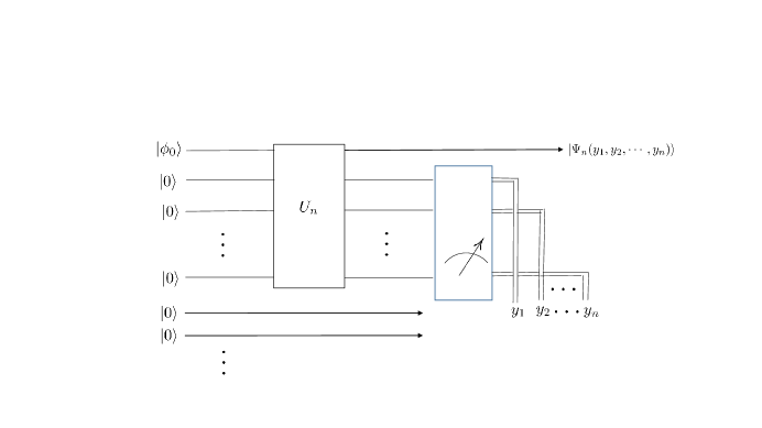
Figure 1: Evolution of the initial state $|\phi_{0}\otimes\Omega_{0}\rangle$ in $\mathcal{H}=\mathcal{H}_{S}\otimes\mathcal{H}_{R}$, induced by a unitary operator $U_{n}$ (see (5)), followed by a measurement on the reservoir yielding a classical output $(y_{1},y_{2},\cdots,y_{n})$ and a post measured state $|\Psi_{n}(y_{1},y_{2},\cdots y_{n})\rangle_{S}$ of the system.

Alternatively, allowing a 1-step evolution by $U_{01}$ on the initial state $|\phi_{0}\otimes 0\rangle$ and making a measurement, we get a classical output $y_{1}$ and a collapsed state $|\Psi_{1}(y_{1})\rangle_{S}$ of the system $S$ given by

$$|\Psi_{1}(y_{1})\rangle_{S}=\frac{L_{y_{1}\,0}\,|\,\phi_{0}\rangle}{||\,L_{y_{1}\,0}\,\phi_{0}||}.$$ (11)

Now, allow this collapsed state to undergo a one-step evolution again, and make a measurement. We get a classical output $y_{2}$ and a collapsed state $|\Psi_{2}(y_{1},y_{2})\rangle_{S}$ given by

$$|\Psi_{2}(y_{1},y_{2})\rangle_{S}=\frac{L_{y_{2}\,0}\,|\Psi_{1}(y_{1})\rangle_{S}}{||\,L_{y_{2}\,0}\,\Psi_{1}(y_{1})||}=\frac{L_{y_{2}\,0}\,L_{y_{1}\,0}\,|\,\phi_{0}\rangle}{||L_{y_{2}\,0}\,L_{y_{1}\,0}\,\phi_{0}||}.$$ (12)

Repeating this procedure $n$ times, we get a classical output sequence $(y_{1},y_{2},\cdots,y_{n})$ and the collapsed state $|\Psi_{n}(y_{1},y_{2},\cdots,y_{n})\rangle_{S}$ of the system, given by the same expression as in (10). Furthermore,

$$|\Psi_{n+1}(y_{1},y_{2},\cdots,y_{n+1})\rangle_{S}=\frac{\,L_{y_{n+1}\,0}\,|\,\Psi_{n}(y_{1},y_{2},\cdots y_{n})\rangle_{S}}{||L_{y_{n+1}\,0}\,\Psi_{n}(y_{1},y_{2},\cdots y_{n})||}.$$ (13)

Thus the sequence $\{|\Psi_{n}(y_{1},y_{2},\cdots,y_{n})\rangle_{S},n=1,2,\cdots\}$ of $\mathcal{H}_{S}$-valued random variables is a Markovian sequence Gisin ; Carm ; Molmer1 ; Molmer2 ; Massen2 , adapted to the random trajectory $(y_{1},y_{2},\cdots)$ of the reservoir, occurring as a classical stochastic process in the wake of successive measurements.

Put

$$\nu_{n}(y_{1},y_{2},\ldots,y_{n})=||L_{y_{n}\,0}\cdots L_{y_{2}\,0}\,L_{y_{1}\,0}\,\phi_{0}||^{2}$$

and observe that

$$\sum_{(y_{1},y_{2},\cdots,y_{n})\in\mathbb{X}^{n}}\,\nu_{n}(y_{1},y_{2},\ldots,y_{n})=1.$$

Moreover,

$$\sum_{y_{n+1}\in\mathbb{X}}\,\nu_{n+1}(y_{1},y_{2},\ldots,y_{n},y_{n+1})=\nu_{n}(y_{1},y_{2},\ldots,y_{n}),$$

for $n=1,2,\cdots$. In other words, $\nu_{n}$ is a probability distribution on $\mathbb{X}^{n}$, which is also the marginal distribution of $\nu_{n+1}$ on the product of the first $n$ copies of $\mathbb{X}$. Thus, $\{\nu_{n}\}$ is a consistent family of distributions over $\{\mathbb{X}^{n}\}$. By Kolmogorov’s consistency theorem, there exists a unique probability measure $\nu_{\infty}$ in the countable product space $\Omega=\mathbb{X}^{\infty}$, whose marginal on the product of the first $n$ copies of $\mathbb{X}$ is $\nu_{n}$ for every $n=1,2,\cdots$. The probability measure $\nu_{\infty}$ describes the statistics of the discrete measurement sequence $(y_{1},y_{2},\cdots)$. Putting

$$Z_{n}(\mathbf{y})=k^{n}\,\nu_{n}(y_{1},y_{2},\cdots,y_{n}),\ n=1,2,\cdots,\mathbf{y}=\omega\in\Omega,$$

we obtain the likelihood ratio martingale sequence $\{Z_{n}\}$ in the probability space $(\Omega,\mu)$. The sequence $\{Z_{n}\}$ is a non-negative martingale, with $\mathbb{E}_{\mu}\,[Z_{n}]=1$, for all $n$. However, there is no guarantee that $\nu_{\infty}$ is absolutely continuous with respect to $\mu$. Thus, the martingale $\{Z_{n}\}$ need not converge to a finite random variable. A simple computation shows that

$$\sum_{(y_{1},y_{2},\cdots,y_{n})\in\mathbb{X}^{n}}\, \left|\Psi_{n}(y_{1},y_{2},\cdots,y_{n})\right\rangle\left\langle\Psi_{n}(y_{1},y_{2},\cdots,y_{n})\right|\ \nu_{n}(y_{1},y_{2},\cdots,y_{n})$$

$$= \int_{\Omega}\,\left|\Psi_{n}(y_{1},y_{2},\cdots,y_{n})\right\rangle\left\langle\Psi_{n}(y_{1},y_{2},\cdots,y_{n})\right|\,\nu_{\infty}(d\mathbf{y})$$

$$= \int_{\Omega}\,\left|\Psi_{n}(y_{1},y_{2},\cdots,y_{n})\right\rangle\left\langle\Psi_{n}(y_{1},y_{2},\cdots,y_{n})\right|\,Z_{n}(\mathbf{y})\,\mu(d\mathbf{y}),$$

where $\nu_{\infty}(d\mathbf{y})$ gets replaced by $Z_{n}(\mathbf{y})\,\mu(d\mathbf{y})$ for all $n=1,2,\cdots.$

This summarizes the way the discrete time irreversible dynamics is determined by the discrete time state-valued Markov chain $\{|\Psi_{n}(\cdot)\rangle\}$ starting from $|\phi_{0}\otimes\Omega_{0}\rangle$. Furthermore, this suggests a natural route for an extension to the continuous time irreversible dynamics described by a quantum dynamical semigroup $\{T_{t},t\geq 0\}$ with GKSL generator $\mathcal{L}$. We can replace the discrete Schrödinger evolution $\{U_{n},n=0,1,2,\cdots\}$ by the HP unitary dilation $\{U(t),t\geq 0\}$ of $\{T_{t},t\geq 0\}$ in the tensor product of $\mathcal{H}_{S}$ with an appropriate Boson Fock space $\mathcal{H}_{R}$, and transfer it to $\mathcal{H}_{S}\otimes L^{2}(\mu)$ with $\mu$ as the Wiener probability measure of a suitable multidimensional Brownian motion $\{\mathbf{B}(t),\,t\geq 0\}$, using the Wiener-Itô-Segal isomorphism. Putting $|\psi_{t}\rangle=U(t)\,|\phi_{0}\otimes\Omega_{0}\rangle$, with $|\phi_{0}\rangle\in\mathcal{H}_{S}$, $|\Omega_{0}\rangle$ being the constant function in $L^{2}(\mu)$, identically equal to unity, and normalizing $|\psi_{t}\rangle$ in $\mathcal{H}_{S}$, we shall arrive at a state diffusion process $\{|\Psi_{t}(\mathbf{B})\rangle,t\geq 0\},$ which is a perfect continuous time analogue of the Markov chain $\{|\Psi_{n}(\cdot)\rangle\}$ given by (11)-(13).

III Boson Fock space and quantum stochastic evolutions

We begin with some general observations on the Boson Fock space $\Gamma(\mathfrak{h})$ over a Hilbert space $\mathfrak{h}$ defined by

$$\Gamma(\mathfrak{h})=\mathbb{C}\oplus\mathfrak{h}\oplus\mathfrak{h}^{ⓢ^{2}}\oplus\cdots\oplus\mathfrak{h}^{ⓢ^{r}}\oplus\cdots$$ (14)

where $\mathbb{C}$ denotes the one dimensional complex Hilbert space and $ⓢ^{r}$ indicates $r$-fold symmetric tensor product of copies of $\mathfrak{h}$. To each $u\in\mathfrak{h}$, its associated exponential vector $e(u)$ is defined by

$$e(u)=1\oplus u\oplus\frac{u^{\otimes^{2}}}{\sqrt{2!}}\oplus\cdots\oplus\frac{u^{\otimes^{r}}}{\sqrt{r!}}\oplus\cdots.$$ (15)

The linear manifold generated by all such exponential vectors is denoted by $\mathcal{E}$. Any finite set of exponential vectors is linearly independent and $\mathcal{E}$ is dense in $\Gamma(\mathfrak{h})$. This implies that any map from the set of all exponential vectors into $\Gamma(\mathfrak{h})$ extends to an operator in $\Gamma(\mathfrak{h})$ with domain $\mathcal{E}$. Any isometry on the set of exponential vectors extends to an isometry on $\Gamma(\mathfrak{h})$. The map $u\rightarrow e(u)$ is strongly continuous and for all $u,\,\,v\in\mathfrak{h}$

$$\langle e(u)|e(v)\rangle={\rm exp}\langle u|v\rangle.$$ (16)

Any element of the subspace $\mathfrak{h}^{ⓢ^{r}}$ in $\Gamma(\mathfrak{h})$ is called an $r$-particle vector. The linear manifold $\mathcal{M}$ generated by $\bigcup\mathfrak{h}^{ⓢ^{r}}$ in $\Gamma(\mathfrak{h})$ is called the manifold of finite particle vectors. To any $u\in\mathfrak{h}$, there is associated a pair of operators $a(u)$, $a^{\dagger}(u)$, defined on the linear manifold $\mathcal{M}$, which are closable (with their corresponding closures denoted by the same symbols) and are called the creation-annihilation pairs associated with $u$. Then, $\mathcal{E}$ is contained in the domain of $a(u)$ and $a^{\dagger}(u)$. These operators are adjoint to each other on $\mathcal{M}$ and $\mathcal{E}$. They enjoy very important properties and the algebra generated by them gives rise to a rich family of observables.

The map $u\rightarrow a(u)$ is antilinear whereas $u\rightarrow a^{\dagger}({u})$ is linear. The operator $a(u)+a^{\dagger}(u)$ closes to a selfadjoint operator and therefore, yields an observable. The linear manifolds $\mathcal{M}$ and $\mathcal{E}$ are in the domain of products of all operators of the form $F_{1},F_{2},\cdots,F_{l}$ where each $F_{i}$ is either $a(u_{i})$ or $a^{\dagger}(u_{i})$ for each $i=1,2,\cdots l$. On both $\mathcal{M}$ and $\mathcal{E}$ the creation and annihilation operators obey the canonical commutation relations:

$$\ [a(u),\,a(v)] = 0,$$

$$\ [a^{\dagger}(u),\,a^{\dagger}(v)] = 0,$$ (17)

$$\ [a(u),\,a^{\dagger}(v)] = \langle u|v\rangle.$$

Furthermore,

$$a(u)\,e(v)=\langle u|v\rangle\,e(v),\ \forall\ \ u,v\in\mathfrak{h}.$$ (18)

If $\mathfrak{h}_{1},\ \mathfrak{h}_{2}$ are two Hilbert spaces, the correspondence

$$e(u_{1}\oplus u_{2})\rightarrow e(u_{1})\otimes e(u_{2}),\ \ \forall\ \,u_{i}\in\mathfrak{h}_{i},i=1,2$$ (19)

extends to a Hilbert space isomorphism between $\Gamma(\mathfrak{h}_{1}\oplus\mathfrak{h}_{2})$ and $\Gamma(\mathfrak{h}_{1})\otimes\Gamma(\mathfrak{h}_{2})$.

Now we specialize to the case where $\mathfrak{h}=L^{2}(\mathbb{R}_{+},\mathbb{C}^{n})=L^{2}(\mathbb{R}_{+})\otimes\mathbb{C}^{n}$, where $L^{2}(\mathbb{R}_{+})$ is the Hilbert space of absolutely square integrable functions on the half-interval $\mathbb{R}_{+}=[0,\infty)$, with respect to the Lebesgue measure and $\mathbb{C}^{n}$ denotes the standard $n$-dimensional complex Hilbert space. The Hilbert space $L^{2}(\mathbbm{R}_{+})\otimes\mathbb{C}^{n}$ can be viewed as the space of $\mathbb{C}^{n}$-valued norm square integrable functions on $\mathbb{R}_{+}$. Any element $\mathbf{u}\in L^{2}(\mathbb{R}_{+})\otimes\mathbb{C}^{n}$ may be expressed as,

$$\mathbf{u}=u_{1}\oplus u_{2}\oplus\cdots\oplus u_{n},\ \ \ \ \ \ u_{k}\in L_{2}(\mathbb{R}_{+}),\ k=1,2,\cdots,n.$$

With any $\mathbf{u}\in L^{2}(\mathbb{R}_{+})\otimes\mathbb{C}^{n}$, we associate the exponential vector $e(\mathbf{u})$ in $\Gamma(L^{2}(\mathbb{R}_{+})\otimes\mathbb{C}^{n})$. For any $\mathbf{u}$ and $\mathbf{v}$ in $L^{2}(\mathbb{R}_{+})\otimes\mathbb{C}^{n}$ we have

$$\langle e(\mathbf{u})|e(\mathbf{v})\rangle = {\rm exp}\langle\mathbf{u}|\mathbf{v}\rangle$$ (20)

$$= {\rm exp}\left[\sum_{k=1}^{n}\,\int_{0}^{\infty}\,u_{k}^{*}\,v_{k}\,dt\right].$$

The vacuum vector $e(\mathbf{\mathbf{0}})=1\oplus\mathbf{0}\oplus\mathbf{0}\oplus\cdots$ in $\Gamma(L^{2}(\mathbb{R}_{+})\otimes\mathbb{C}^{n})$ is denoted by $\Omega_{0}$.

We consider a quantum system $S$ in a Hilbert space $\mathcal{H}_{S}$, coupled to a reservoir $R$ in a Boson Fock space $\mathcal{H}_{R}=\Gamma(L^{2}(\mathbbm{R}_{+})\otimes\mathbb{C}^{n})$. The global Hilbert space $\mathcal{H}=\mathcal{H}_{S}\otimes\mathcal{H}_{R}$ is used to describe events, observables and states of the system plus reservoir. The noise processes can be described by observables in the general continuous tensor product Hilbert space of the reservoir for which the Boson Fock space $\Gamma(L^{2}(\mathbbm{R}_{+})\otimes\mathbb{C}^{n})$ serves as one of the simplest models. The space $\mathbb{C}^{n}$ corresponds to $n$ degrees of freedom in the selection of noise.

For any $0<t_{1}<t_{2}\cdots<t_{r}<\infty$, we have the following decomposition of $\mathcal{H}=\mathcal{H}_{S}\otimes\mathcal{H}_{R}$:

$$\mathcal{H}([0,t)) = \mathcal{H}_{S}\otimes\Gamma(L^{2}([0,t))\otimes\mathbb{C}^{n})$$

$$\mathcal{H}([t_{r-1},t_{r})) = \Gamma(L^{2}([t_{r-1},t_{r}))\otimes\mathbb{C}^{n})$$

$$\mathcal{H}([t_{r},\infty)) = \Gamma(L^{2}([t_{r},\infty))\otimes\mathbb{C}^{n})$$

and we denote the restrictions of $\mathbf{u}$ to the time intervals $[0,t]$, $[t_{1},t_{2})$, and $[t_{r},\infty)$ by

$$\left.\mathbf{u}\right|_{[0,t)} = \mathbf{u}_{t]},$$

$$\left.\mathbf{u}\right|_{[t_{r-1},t_{r})} = \mathbf{u}_{[t_{r-1},t_{r})},$$

$$\left.\mathbf{u}\right|_{[t_{r},\infty)} = \mathbf{u}_{[t_{r}}.$$

From the correspondence given by (19), it follows that, there exists a unique unitary isomorphism $\mathcal{U}:\mathcal{H}\rightarrow\mathcal{H}([0,t_{1}))\otimes\mathcal{H}([t_{1},t_{2}))\otimes\cdots\otimes\mathcal{H}([t_{r-1},t_{r}))\otimes\mathcal{H}([t_{r},\infty))$ satisfying,

$$\mathcal{U}\,\phi\otimes e(\mathbf{u})=\phi\otimes e(\mathbf{u}_{t_{1}]}))\otimes e(\mathbf{u}_{[t_{1},t_{2})})\otimes\cdots\otimes e(\mathbf{u}_{[t_{r-1},t_{r})})\otimes e(\mathbf{u}_{[t_{r}})\\$$ (21)

for all $\phi\in\mathcal{H}_{S}$ and $e(\mathbf{u})\in\mathcal{H}_{R}$.

Using the notions of creation and annihilation operators introduced in (III), (18), we consider the family of linear operators $\{A_{k}(t),t\geq 0\}$ and $\{A^{\dagger}_{k}(t),t\geq 0\}$ as follows:

$$A_{k}(t) = I_{S}\otimes a\left(1_{[0,t]}\otimes|k\rangle\right)$$ (22)

$$A^{\dagger}_{k}(t) = I_{S}\otimes a^{\dagger}\left(1_{[0,t]}\otimes|k\rangle\right)$$ (23)

where $\{|k\rangle=(0,\cdots,0,1,0,\cdots,0)\}$ (with $1$ in the $k$-th place), $k=1,2,\cdots,n$, is a canonical orthonormal basis in $\mathbb{C}^{n}$; $1_{[0,t]}$ denotes the indicator function of the interval $[0,t]$ for each $t\in\mathbb{R}_{+}$ and $I_{S}$ denotes the identity operator in $\mathcal{H}_{S}$. The operators defined in (22) and (23) obey the canonical commutation relations (CCRs):

$$\,[A_{k}(s),A_{l}(t)] = 0=[A^{\dagger}_{k}(s),A^{\dagger}_{l}(t)],$$ (24)

$$\,[A_{k}(s),A^{\dagger}_{l}(t)] = \delta_{kl}\,(s\wedge t)\,I_{S}\otimes I_{R}.$$ (25)

Here $s\wedge t$ denotes the minimum of $s$ and $t$.

The operators $A_{k}(t),\ A^{\dagger}_{k}(t)$ are well-defined on the linear manifold generated by elements of the form $\phi\otimes e(\mathbf{u}),$ with $\phi\in\mathcal{H}_{S}$ and $\mathbf{u}\in L^{2}(\mathbb{R}_{+}\otimes\mathbb{C}^{n})$. In particular, one obtains the following eigen-relation for $A_{k}(t)$:

$$A_{k}(t)\,|\phi\otimes e(\mathbf{u})\rangle = \left(\int_{0}^{t}u_{k}(s)\,ds\,\right)\,\,|\phi\otimes e(\mathbf{u})\rangle$$ (26)

and consequently, the adjoint relation for $A^{\dagger}_{k}(t)$ follows:

$$\langle\phi\otimes e(\mathbf{u})|A^{\dagger}_{k}(t) = \langle\phi\otimes e(\mathbf{u})|\left(\int_{0}^{t}u^{*}_{k}(s)\,ds\,\right).$$ (27)

The family of operators $\{A_{k}(t),t\geq 0\}$, $\{A^{\dagger}_{k}(t),t\geq 0\}$ are respectively called the annihilation and creation processes. These are the fundamental noise processes of quantum stochastic calculus. (For more detailed description of fundamental noise processes in Boson Fock space, including conservation noise process, see Refs. HP ; KRP ).

A family $X=\left\{X(t),0\leq t<\infty\right\}$ of operators in $\mathcal{H}$ is said to be adapted if, for each $t,$ there exists an operator $X_{t}$ in $\mathcal{H}([0,t))$ such that

$$X(t)=X_{t}\otimes I_{[t}$$

where $I_{[t}$ is the identity operator in $\mathcal{H}([t,\infty)).$ Further, an adapted process $X$ is said to be simple with respect to a partition $0<t_{1}<t_{2}<\cdots<t_{r}<\cdots$ of $[0,\infty)$ such that $t_{r}\rightarrow\infty$ as $r\rightarrow\infty$, if

$$X(t)=X({t_{j}})\ \ {\rm when}\ t_{j}\leq t<t_{j+1},\ \ j=0,1,2,\cdots.$$ (28)

Let $\{L(t)\}$ be such a simple adapted process and $\{M(t)\}$ be any one of the fundamental operator-valued adapted processes $\{A_{k}(t)\}$, $\{A_{k}^{\dagger}(t)\},\ k=1,2,\cdots,n$. Then, the stochastic integral of $\{L(t)\}$, with respect to $\{M(t)\}$ is defined by

$$X(t) = \int_{0}^{t}\,L(s)\,d\,M(s)$$

$$= \sum_{t_{j}}\,L_{t_{j}}\,\left(M(t_{j+1}\wedge t)-M(t_{j}\wedge t)\right),$$

$$\ \ \ \ \ \ \ \ \ \ \ t_{j}\leq t<t_{j+1},\ \ \ j=0,1,2,\cdots.$$

It may be noted that the operators $L_{t_{j}}$ and $M(t_{j+1}\wedge t)-M(t_{j}\wedge t)$ commute with each other i.e., $L(s)\,d\,M(s)$ can be written as $d\,M(s)\,L(s).$

As shown in Ref. HP , the notion of such integrals can be extended by a completion procedure to a wide class of adapted processes, which are not necessarily simple. Such an integration is a linear operation in the space of adapted processes. For details see Sec. 4 of Ref. HP .

We consider adapted processes of the form

$$X(t)=X(0)+\int_{0}^{t}\,\sum_{k=1}^{n}\,\left(E_{k}(s)\,dA^{\dagger}_{k}(s)\,+F_{k}(s)\,dA_{k}(s)+G_{k}(s)\,ds\right)$$ (30)

where $X(0)=X_{0}\otimes I_{R}$, $X_{0}$ is an operator in the system Hilbert space $\mathcal{H}_{S}$ and $I_{R}$ denotes the identity operator in $\mathcal{H}_{R}$; the integrands $E_{k}(t),F_{k}(t),G_{k}(t)$ are adapted processes. We write (30) in the differential form as,

$$dX(t)=\sum_{k=1}^{n}\,\left(E_{k}(t)dA^{\dagger}_{k}(t)\,+F_{k}(t)\,dA_{k}(t)+\,G_{k}(t)\,dt\right),$$ (31)

with initial value $X_{0}\otimes I_{R}$.

The central result of quantum stochastic calculus is the following quantum Itô multiplication table HP ; KRP , summarized as follows:

   $$dA^{\dagger}_{k}\hskip 7.22743pt$$        

    0 0 0

0 0

0 0 0

(32)

The product of two stochastic integrals is again a stochastic integral, the differentials of which satisfy the modified Leibnitz relation,

$$d(X\,Y)=(dX)\,Y+X\,(dY)+\,(dX)\,(dY).$$ (33)

Quantum Itô multiplication table (32) is employed in (33) to express the differential $d(X\,Y)$ of the product of adapted processes $X$, $Y$ in terms of the fundamental operator-valued differentials $dA^{\dagger}_{k},\,dA_{k}$ and $dt$. This provides a simple and natural extension of Itô calculus based on Brownian motion McKean to its quantum counterpart in the Boson Fock space.

One of the most successful applications of HP quantum stochastic calculus is the realization of unitary dilations of quantum dynamical semigroups through Schrödinger evolutions of open systems. Such a Schrödinger evolution can be expressed through a unitary operator-valued process obeying a quantum stochastic differential equation of the form,

$$dU(t)=\left(\sum_{k=1}^{n}\,\left(L^{(1)}_{k}\,dA^{\dagger}_{k}(t)+L^{(2)}_{k}\,dA_{k}(t)\right)+L^{(3)}\,dt\right)\!U(t),\ \ \ U(0)=I$$ (34)

in $\mathcal{H}=\mathcal{H}_{S}\otimes\mathcal{H}_{R}$, where $L^{(\alpha)}_{k},\ \alpha=1,2,3$ are bounded operators in $\mathcal{H}_{S}$. It is shown HP that a unique unitary solution for (34) exists if

$$L^{(1)}_{k} = L_{k},L^{(2)}_{k}=-L^{\dagger}_{k}$$

$$L^{(3)}_{k} = -i\,H-\frac{1}{2}\,\sum_{k=1}^{n}\,L_{k}^{\dagger}\,L_{k}$$ (35)

and $H$ is a self-adjoint operator. Taking the conditions (35) into account, (34) can be expressed as HP ; KRP

$$dU(t)=\left[\sum_{k=1}^{n}\,\left(L_{k}\,dA^{\dagger}_{k}(t)-L^{\dagger}_{k}\,dA_{k}(t)\right)-\left(i\,H+\frac{1}{2}\,\sum_{k=1}^{n}\,L_{k}^{\dagger}\,L_{k}\right)\,dt\right]\!U(t),\ \ \ U(0)=I,$$ (36)

which is referred to as the HP equation. In terms of the set of operators $\mathbf{L}=(L_{1},L_{2},\cdots,L_{n})$ and $H$, we denote the unitary process $\{U(t),t\geq 0\}$ satisfying (36) by $U\!(\mathbf{L},H)$. In the special case of $L_{k}=0$ for all $k=1,2,\cdots,n$, one obtains the familiar Schrödinger unitary dynamics

$$dU(t)=-i\,H\,U(t),$$ (37)

with $H$ being the Hamiltonian of the quantum system. It is of interest to note that there do exist examples with unique unitary solutions, when the coefficients $L_{k}$ and $H$ in (36) are unbounded Fan ; Fan&Wills ; Fan13 ; KRPG .

We may now use the unitary process $\{U(t),t\geq 0\}$ to describe noisy Heisenberg dynamics. To this end, consider any bounded operator $X$ in the system Hilbert space $\mathcal{H}_{S}$ (i.e., $X\in\mathcal{B}(\mathcal{H}_{S})$), and a unitary process $U\!(\mathbf{L},H)$. Define a homomorphism $j_{t}:\ \mathcal{B}(\mathcal{H}_{S})\longrightarrow\mathcal{B}(\mathcal{H}_{S}\otimes\mathcal{H}_{R})$ by

$$j_{t}(X)=U(t)^{\dagger}(X\otimes I_{R})U(t),\quad t\geq 0.$$ (38)

Using the relation (33) and employing the quantum Itô multiplication table given by (32), one obtains

$$dj_{t}(X)=\sum_{k=1}^{n}\,\left\{\,j_{t}\left([X,L_{k}]\right)\,dA^{\dagger}_{k}(t)-j_{t}\left([X,L_{k}^{\dagger}]\right)\,dA_{k}(t)\right\}+j_{t}\left(\mathcal{L}(X)\right)\,dt,$$ (39)

where the map $\mathcal{L}$ from $\mathcal{B}(\mathcal{H}_{S})$ to itself is given by

$$\mathcal{L}(X) = i\left[H,\,X\right]-\frac{1}{2}\sum_{k=1}^{n}\left(L^{\dagger}_{k}\,L_{k}\,X+X\,L^{\dagger}_{k}\,L_{k}-2\,L^{\dagger}_{k}\,X\,L_{k}\right)$$ (40)

Equation (39) describes noisy evolution of system observables $X$. If $L_{k}=0\ \ \ \forall\ \,k,$ then (39) reduces to the well-known Heisenberg equation of motion for the observable $X$:

$$\frac{dj_{t}(X)}{dt}=j_{t}(i[H,X]).$$

For any operator $F$ in $\mathcal{H}$ we define the vacuum conditional expectation value as the unique operator $\mathbb{E}_{\Omega_{0}}(F)$ in $\mathcal{H}_{S}$ determined by,

$$\langle\phi|\mathbb{E}_{\Omega_{0}}(F)|\chi\rangle=\langle\phi\otimes\Omega_{0}|F|\chi\otimes\Omega_{0}\rangle,\ \ \forall\,\,\ \phi,\chi\in\mathcal{H}_{S}.$$ (41)

Now, we write the vacuum conditional expectation value of $j_{t}(X)$ as

$$\mathbb{E}_{\Omega_{0}}\left(j_{t}(X)\right) = \mathbb{E}_{\Omega_{0}}\,\left(U(t)^{\dagger}(X\otimes I_{R})U(t)\right)$$ (42)

$$= T_{t}(X)$$

Thus one obtains

$$\frac{dT_{t}(X)}{dt}=T_{t}(\mathcal{L}(X))=\mathcal{L}\left(T_{t}(X)\right)$$ (43)

for the time evolution of the quantum dynamical semigroup of completely positive unital maps

$$T_{t}={\rm exp}(t\,\mathcal{L}),\ \ t\geq 0$$ (44)

on $\mathcal{B}(\mathcal{H}_{S})$ generated by $\mathcal{L}$ of (40). This coincides with the well-known form obtained by Gorini, Kossakowski, Sudarshan Gorini and Lindblad Lindblad .

For the initial state $\rho_{0}\otimes|\Omega_{0}\rangle\langle\Omega_{0}|$ of the system plus reservoir, we express,

$${\rm Tr}\left(\rho_{0}\otimes|\Omega_{0}\rangle\langle\Omega_{0}|\,j_{t}(X)\right) = {\rm Tr}\left(\rho_{0}\,T_{t}(X)\right)$$ (45)

$$= {\rm Tr}\left(\rho_{t}\,X\right),$$

where $\rho_{t}={\rm Tr}_{R}\left(U(t)\,\rho_{0}\otimes|\Omega_{0}\rangle\langle\Omega_{0}|\,U(t)^{\dagger}\right)$ denotes the reduced density operator of the quantum system. Using (42)-(45) we get the Gorini-Kossakowski-Sudarshan-Lindblad (GKSL) master equation for $\rho_{t}$ :

$$\frac{d\rho_{t}}{dt}=-i[H,\,\rho_{t}]-\frac{1}{2}\sum_{k=1}^{n}\left(L^{\dagger}_{k}\,L_{k}\,\rho_{t}+\rho_{t}\,L^{\dagger}_{k}\,L_{k}-2\,L_{k}\,\rho_{t}\,L^{\dagger}_{k}\right).$$ (46)

In the next section we discuss invariance properties of the GKSL generator $\mathcal{L}$.

IV Symmetries of the GKSL generator

Let $\{R_{i}(t)=I_{S}\otimes F_{i}(t),t\geq 0\},\ i=1,2$ be unitary adapted processes in $\mathcal{H}$ such that $\{F_{i}(t),t\geq 0\},\,i=1,2$, act only on the reservoir space $\mathcal{H}_{R}$. Let

$$F_{2}(t)|\,\Omega_{0}\rangle=F_{2}(t)^{\dagger}\,|\Omega_{0}\rangle=|\Omega_{0}\rangle\,,\ \ t\geq 0.$$ (47)

Consider the process

$$\{V(t)=R_{1}(t)\,U(t)\,R_{2}(t),\ t\geq 0\}$$ (48)

where $U(t)$ satisfies the HP equation (36). Define a homomorphism $j^{\prime}_{t}:\ \mathcal{B}(\mathcal{H}_{S})\longrightarrow\mathcal{B}(\mathcal{H}_{S}\otimes\mathcal{H}_{R})$ by

$$j^{\prime}_{t}(X)=V^{\dagger}(t)(X\otimes I_{R})V(t),\quad t\geq 0.$$ (49)

Then, the vacuum conditional expectation value (see (41) and (42)) of $j^{\prime}_{t}(X)$ is given by,

$$\mathbb{E}_{\Omega_{0}}\left(j^{\prime}_{t}(X)\right) = \mathbb{E}_{\Omega_{0}}\,\left(R^{\dagger}_{2}(t)\,U^{\dagger}(t)\,R^{\dagger}_{1}(t)(X\otimes I_{R})R_{1}(t)\,U(t)\,R_{2}(t)\right)$$ (50)

$$= \mathbb{E}_{\Omega_{0}}\,\left(U^{\dagger}(t)\,(X\otimes I_{R})U(t)\,\right)=\mathbb{E}_{\Omega_{0}}\left(j_{t}(X)\right)=T_{t}(X)=e^{t\,\mathcal{L}}(X).$$

for all $t\geq 0$ and $X$ in $\mathcal{B}(\mathcal{H}_{S})$. Thus, conjugation by the unitary adapted processes $\{U(t)\}$ and $\{V(t)\}$ yield the reduced dynamics of the quantum system with the same GKSL generator $\mathcal{L}$. In the following, we discuss two important examples of $\{V(t),t\geq 0\}$, which specialize to the translation and rotation invariance of the GKSL generator $\mathcal{L}$.

IV.1 Example 1

In analogy with exponential vectors of (15) we now introduce exponential operators in $\mathcal{H}_{R}$ as follows: For any $\mathbf{f}\in L^{2}(\mathbb{R}_{+})\otimes\mathbb{C}^{n}$, we write, on the set of exponential vectors,

$$W(\mathbf{f})e(\mathbf{u})=e^{-\frac{1}{2}||\mathbf{f}||^{2}-\langle\mathbf{f}|\mathbf{u}\rangle}e(\mathbf{f}+\mathbf{u})\quad\forall\,\ \mathbf{u}\in\mathcal{K},$$ (51)

where $||\mathbf{f}||^{2}=\int_{0}^{\infty}|\mathbf{f}|^{2}\,dt,$ and $|\mathbf{f}|^{2}=\sum_{k=1}^{n}\,|f_{k}|^{2}$. The exponential operator $W(\mathbf{f})$ preserves the scalar product between exponential vectors and therefore extends to a unique unitary operator in $\mathcal{H}_{R}$, which we denote by the same symbol $W(\mathbf{f})$.

A normalized vector $\alpha(\mathbf{f})\in\mathcal{H}_{R}$ given by

$$\alpha(\mathbf{f}) = W(\mathbf{f})\,e(\mathbf{0})=e^{-\frac{1}{2}||\mathbf{f}||^{2}}\,e(\mathbf{f}),\ \ \mathbf{f}\in L^{2}(\mathbb{R_{+}})\otimes\mathbb{C}^{n},$$ (52)

is called a coherent state associated with $\mathbf{f}$.

The operators $W(\mathbf{f}),\ W(\mathbf{g})$ obey the multiplication relation,

$$W(\mathbf{f})W(\mathbf{g})=e^{-i\,\,{\rm Im}\langle\mathbf{f}|\mathbf{g}\rangle}\,W(\mathbf{f}+\mathbf{g}),\ \ \forall\,\ \mathbf{f},\mathbf{g}\in\mathcal{K}.$$ (53)

These are the well known Weyl canonical commutation relations (CCRs) of which the CCRs of creation and annihilation operators ( III) are the infinitesimal versions. We call $W(\mathbf{f})$ the Weyl displacement operator associated with $\mathbf{f}.$

Now, for any map $\mathbf{f}:\mathbb{R}_{+}\rightarrow\mathbb{C}^{n}$ satisfying the local square integrability condition

$$\int_{0}^{t}\,|\mathbf{f}(s)|^{2}\,ds<\infty,\ \forall\,\ t>0$$

we introduce the unitary Weyl displacement operator process $\{W(\mathbf{f})(t),t\geq 0\}$ by the relation

$$W(\mathbf{f})(t)\,e(\mathbf{u})=W(1_{[0,t]}\mathbf{f})\,e(\mathbf{u}_{t]})\otimes e(\mathbf{u}_{[t}).$$ (54)

Then $\{R_{\mathbf{f}}(t)=I_{S}\otimes W(\mathbf{f})(t),t\geq 0\}$ is a unitary adapted process in $\mathcal{H}_{S}\otimes\mathcal{H}_{R}$, which obeys the quantum stochastic differential equation

$$dR_{\mathbf{f}}(t)=\left\{\sum_{k=1}^{n}\,\left(f_{k}\,dA^{\dagger}_{k}(t)-f_{k}^{*}dA_{k}(t)\right)-\frac{1}{2}\,\sum_{k=1}^{n}\,|f_{k}|^{2}\,dt\right\}\!R_{\mathbf{f}}(t),\ \ t\geq 0$$ (55)

with initial condition $R_{\mathbf{f}}(0)=I_{S}\otimes I_{R}$.

Choose $R_{1}(t)=R_{\mathbf{f}}(t)$, $R_{2}=I_{S}\otimes I_{R}$ in (48). Then, $\{V(t)=R_{\mathbf{f}}(t)\,U(t),t\geq 0\}$, is a unitary adapted process satisfying

$$dV(t) = \left[dR_{\mathbf{f}}(t)\right]U(t)+R_{\mathbf{f}}(t)\left[dU(t)\right]+\left[dR_{\mathbf{f}}(t)\right]\,\left[dU(t)\right]$$ (56)

$$= \left\{\sum_{k=1}^{n}\,\left((L_{k}+f_{k})\,dA^{\dagger}_{k}(t)-(L^{\dagger}_{k}+f^{*}_{k})\,dA_{k}(t)\right)\right.$$

$$\hskip 36.135pt\left.-\left(iH+\frac{1}{2}\,\sum_{k=1}^{n}\,(L_{k}^{\dagger}L_{k}+|f_{k}|^{2}+2\,f_{k}^{*}L_{k}\right)\right\}\!V(t)$$

with initial condition $V(0)=I_{S}\otimes I_{R}$. The process $\{V(t),t\geq 0\}$ is, indeed, given by

$$\{V(t),t\geq 0\}=U\left(\mathbf{L}^{\prime},\,H^{\prime}\right),$$

where $\mathbf{L}^{\prime}=\mathbf{L}+\mathbf{f}$ and $H^{\prime}=H+\frac{1}{2i}\sum_{k=1}^{n}\,\left(f_{k}^{*}L_{k}-f_{k}\,L_{k}^{\dagger}\right).$

Clearly, the homomorphism $j_{t,\mathbf{f}}:\ \mathcal{B}(\mathcal{H}_{S})\longrightarrow\mathcal{B}(\mathcal{H}_{S}\otimes\mathcal{H}_{R})$ defined by

$$j_{t,\mathbf{f}}(X)=V(t)^{\dagger}(X\otimes I_{R})V(t)$$

satisfies the relation

$$j_{t,\mathbf{f}}(X)\equiv U(t)^{\dagger}(X\otimes I_{R})U(t)=j_{t}(X)$$

and hence, the generator $\mathcal{L}$, defined by (40) with operators $(\mathbf{L},\,H)$, remains invariant, when $\mathbf{L}$, $H$ are replaced by $\mathbf{L}^{\prime}=\mathbf{L}+\mathbf{f}$ and $H^{\prime}=H+\frac{1}{2i}\,\displaystyle\sum_{k=0}^{n}(f_{k}^{*}L_{k}-f_{k}\,L_{k}^{\dagger})$ respectively.

Remark: When $\mathbf{f}(\cdot)$ is a constant vector $\boldsymbol{\ell}$ for all $t\geq 0$, it follows that $\mathbf{L}^{\prime}=\mathbf{L}+\boldsymbol{\ell}$ and $H^{\prime}=H+\frac{1}{2i}\,\displaystyle\sum_{k=0}^{n}(\ell_{k}^{*}L_{k}-\ell_{k}\,L_{k}^{\dagger})$, thereby exhibiting the translation invariance property of the GKSL generator $\mathcal{L}$.

IV.2 Example 2

Let $t\rightarrow\mathbf{F}(t)$ be an $n\times n$ unitary matrix-valued Borel map on $\mathbb{R}_{+}$. Define the second quantization unitary operator process $\{\Gamma(\mathbf{F})(t),t\geq 0\}$, acting only on $\mathcal{H}_{R}$, by the relation

$$\Gamma(\mathbf{F})(t)\,e(\mathbf{u})=\Gamma(\mathbf{F})(t)\,e(u\otimes\boldsymbol{\zeta})=e\left(u_{t]}\otimes\mathbf{F}(t)\,\boldsymbol{\zeta}\right)\otimes e(u_{[t}\otimes\boldsymbol{\zeta}).$$ (57)

where we use the identification $L^{2}(\mathbb{R}_{+},\mathbb{C}^{n})=L^{2}(\mathbb{R}_{+})\otimes\mathbb{C}^{n}$ and choose $\mathbf{u}=u\otimes\boldsymbol{\zeta}$ with $u\in L^{2}(\mathbf{R}_{+})$ and $\boldsymbol{\zeta}\in\mathbb{C}^{n}$. Then,

$$\Gamma(\mathbf{F})(t)\,\Omega_{0}=\Gamma^{\dagger}(\mathbf{F})(t)\,\Omega_{0}=\Omega_{0}.$$ (58)

Define

$$R(t)=I_{S}\otimes\Gamma(\mathbf{F})(t),\ \ \ t\geq 0.$$ (59)

and choose $R_{1}(t)=R(t)$, $R_{2}(t)=R^{\dagger}(t)$ in (48). Then,

$$V(t)=R(t)\,U(t)\,R^{\dagger}(t),\ t\geq 0.$$

Define the homomorphism $j_{t,\mathbf{F}}:\ \mathcal{B}(\mathcal{H}_{S})\longrightarrow\mathcal{B}(\mathcal{H}_{S}\otimes\mathcal{H}_{R})$ by

$$j_{t,\mathbf{F}}(X) = V^{\dagger}(t)(X\otimes I_{R})V(t)$$ (60)

$$= I_{S}\otimes\Gamma(\mathbf{F})(t)\,U^{\dagger}(t)(X\otimes I_{R})U(t)\,I_{S}\otimes\Gamma^{\dagger}(\mathbf{F})(t),\ \forall\ \ t\geq 0.$$

Then, it follows immediately from (58) that,

$$\mathbb{E}_{\Omega_{0}}\left(j_{t,\mathbf{F}}(X)\right) = \mathbb{E}_{\Omega_{0}}\,\left(U^{\dagger}(t)(X\otimes I_{R})U(t)\right)$$ (61)

$$= \mathbb{E}_{\Omega_{0}}\left(j_{t}(X)\right)=e^{t\,\mathcal{L}}(X).$$

In other words, both $\{U(t)\}$ and $\{V(t)=R(t)\,U(t)\,R^{\dagger}(t)\}$ yield the irreversible dynamics of the states and observables of the quantum system with the same GKSL generator $\mathcal{L}$.

Remark: Consider a special case of the second quantization unitary process $\{\Gamma(\mathbf{F}(t)\}$, where $\mathbf{F}(t)$ is a constant $n\times n$ unitary matrix defined by, $\mathbf{F}(t)=((u_{ij})),\ i,j=1,2,\cdots,n$ for all $t\geq 0$. Then, $\{U(t),t\geq 0\}=U(\mathbf{L},H)$ and $\{V(t),t\geq 0\}=U(\mathbf{L}^{\prime},H^{\prime})$, where $L^{\prime}_{i}=\sum_{j=1}^{n}\,u_{ij}\,L_{j},\ \ H^{\prime}=H$. The GKSL generator $\mathcal{L}$ remains invariant, when the operator parameters $(\mathbf{L},H)$ are replaced by $(\mathbf{L^{\prime}},H^{\prime})$, thereby exhibiting the rotation invariance property of $\mathcal{L}$.

V Wiener-Itô-Segal isomorphism

We shall now describe the HP quantum stochastic calculus in the Hilbert space $L^{2}(\mu)$, where $\mu$ is the classical Wiener probability measure of the $n$-dimensional standard Brownian motion process $\{\mathbf{B}(t),t\geq 0\}$. To this end, we denote $\left\{\mathbf{B}(t)^{T}=\left(B_{1}(t),B_{2}(t),\cdots,B_{n}(t)\right)^{T}\right\}$ where $B_{k}(t),$ $1\leq k\leq n$ are $n$ independent one dimensional standard Brownian motion processes, ‘$T$’ denoting transpose. We introduce the exponential random variables

$$\widetilde{e}(\mathbf{u})(\mathbf{B})={\rm exp}\,\left(\int_{0}^{\infty}\mathbf{u}(s)^{T}\,d\mathbf{B}(s)-\frac{1}{2}\,\int_{0}^{\infty}\mathbf{u}(s)^{T}\mathbf{u}(s)\,ds\right),\ \ \mathbf{u}\in L^{2}(\mathbb{R}_{+})\otimes\mathbb{C}^{n},$$ (62)

where we view $L^{2}(\mathbb{R}_{+})\otimes\mathbb{C}^{n}$ also as the direct sum of $n$ copies of $L^{2}(\mathbb{R}_{+}).$ Now, consider the correspondence

$$\Theta:\ e(\mathbf{u})\rightarrow\widetilde{e}(\mathbf{u}),$$

where $e(\mathbf{u})$ is the exponential vector defined in Section III (see (15)). The map $\Theta$ is scalar product preserving and so, it extends uniquely to a Hilbert space isomorphism from the Boson Fock space $\Gamma(L^{2}(\mathbb{R}_{+})\otimes\mathbb{C}^{n})$ to $L^{2}(\mu)$. This is called the Wiener-Itô-Segal isomorphism Wiener ; Ito ; Segal .

For any vector $\phi$ in $\mathcal{H}_{R}=\Gamma(L^{2}(\mathbb{R}_{+})\otimes\mathbb{C}^{n})$ or in $\mathcal{H}=\mathcal{H}_{S}\otimes\mathcal{H}_{R}$, we write

$$\widetilde{\phi}=\left\{\begin{array}[]{l}\Theta\,\phi,\ {\rm if}\ \phi\in\mathcal{H}_{R},\\ I_{S}\otimes\Theta\,\phi,\ {\rm if}\ \phi\in\mathcal{H}.\end{array}\right.$$ (65)

Then $\phi\rightarrow\widetilde{\phi}$ is a Hilbert space isomorphism from $\mathcal{H}_{R}\rightarrow L^{2}(\mu)$ as well as $\mathcal{H}\rightarrow\mathcal{H_{S}}\otimes L^{2}(\mu)$. We shall identify $\mathcal{H_{S}}\otimes L^{2}(\mu)$ with the space $L^{2}(\mu,\mathcal{H}_{S})$ of $\mathcal{H}_{S}$-valued norm square integrable functions on the space of Brownian paths. A typical element of $L^{2}(\mu,\mathcal{H}_{S})$ is a functional $\widetilde{\phi}(\mathbf{B})$ and the scalar product of two vectors $\widetilde{\phi}_{1}$, $\widetilde{\phi}_{2}$ in $L^{2}(\mu,\mathcal{H}_{S})$ is given by,

$$\langle\widetilde{\phi}_{1}|\widetilde{\phi}_{2}\rangle = \mathbb{E}_{\mathbf{B}}[\langle\,\widetilde{\phi}_{1}|\widetilde{\phi}_{2}\rangle_{S}]=\int\,\langle\widetilde{\phi}_{1}(\mathbf{B})|\widetilde{\phi}_{2}(\mathbf{B})\rangle_{S}\ \mu(d\mathbf{B})$$ (66)

where $\langle\cdot|\cdot\rangle_{S}$ denotes scalar product in the system Hilbert space $\mathcal{H}_{S}$ and $\mathbb{E}_{\mathbf{B}}[\cdot]$ denotes expectation value with respect to $\mu$. For any operator $X$ in $\mathcal{H}_{R}$ or $\mathcal{H}$, we write

$$\widetilde{X}=\Theta\,X\,\Theta^{-1}.$$

Denote by $\mu_{[t_{1},t_{2}]}$, $\mu_{[t_{1},\infty)},$ the probability measure of the Brownian motion

$$\{\mathbf{B}(t+t_{1})-\mathbf{B}(t_{1}),\ \ 0\leq t\leq t_{2}-t_{1}\}.$$

It may be noted that the factorizability property

$$L^{2}(\mu)=L_{2}(\mu_{[0,t_{1}]})\otimes L_{2}(\mu_{[t_{1},t_{2}]})\otimes\cdots\otimes L_{2}(\mu_{[t_{r-1},t_{r}]})\otimes L_{2}(\mu_{[t_{r},\infty)}),$$ (67)

holds for all $0<t_{1}<t_{2}<\cdots<t_{r-1}<t_{r}<\infty$. In other words, the isomorphism $\Theta$ between $\mathcal{H}_{R}$ and $L^{2}(\mu)$ preserves the continuous tensor product structure. With the restriction of $\mathbf{u}\in L^{2}(\mathbb{R}_{+})\otimes\mathbb{C}^{n}$ to the time interval $[t_{1},t_{2}]$, $0\leq t_{1}<t_{2}<\infty$, in $\mathbb{R}_{+}$, the exponential random variables in $L^{2}(\mu_{[t_{1},t_{2}]})$ are expressed by

$$\widetilde{e}(\mathbf{u}_{[t_{1},t_{2}]})(\mathbf{B})={\rm exp}\,\left(\int_{t_{1}}^{t_{2}}\mathbf{u}(s)^{T}\,d\mathbf{B}(s)-\frac{1}{2}\,\int_{t_{1}}^{t_{2}}\mathbf{u}(s)^{T}\mathbf{u}(s)\,ds\right).$$ (68)

The Wiener-Itô-Segal isomorphism maps the vacuum vector $\Omega_{0}=e(\mathbf{0})$ of the Boson Fock space to the constant function in $L^{2}(\mu)$, identically equal to unity. Furthermore, we have the following proposition, which identifies the sum of creation and annihilation processes in $\Gamma(L^{2}(\mu)\otimes\mathbb{C}^{n})$ with multiplication by components of the $n$-dimensional Brownian motion in $L^{2}(\mu)$ under the isomorphism $\Theta$.

Proposition: Let

$$Q_{k}(t)=A_{k}(t)+A^{\dagger}_{k}(t),\ \ 0\leq t<\infty$$

in $\Gamma(L^{2}(\mathbb{R}_{+})\otimes\mathbb{C}^{n})$. Then, $\Theta\,Q_{k}(t)\,\Theta^{-1}$ is multiplication by Brownian motion random variable $B_{k}(t)$ in $L^{2}(\mu)$ i.e.,

$$[\,\widetilde{Q}_{k}(t)\,\,\widetilde{\phi}\,]\,(\mathbf{B})=B_{k}(t)\,\widetilde{\phi}\,(\mathbf{B})$$ (69)

for all $\widetilde{\phi}\in L^{2}(\mu,\mathcal{H}_{S})$ under the Wiener-Itô-Segal isomorphism.

Proof: Using (26), (27), we obtain

$$\langle e(\mathbf{u})|Q_{k}(t)|e(\mathbf{v})\rangle = e^{\langle\mathbf{u}|\mathbf{v}\rangle}\,\int_{0}^{t}\,(u^{*}_{k}+v_{k})(s)\,ds,$$ (70)

which yields,

$$\frac{d}{dt}\,\langle e(\mathbf{u})|Q_{k}(t)|e(\mathbf{v})\rangle = e^{\langle\mathbf{u}|\mathbf{v}\rangle}\ \,(u^{*}_{k}+v_{k})(t)$$ (71)

in $\Gamma(L^{2}(\mathbb{R}_{+}\otimes\mathbb{C}^{n}).$

On the other hand,

$$\mathbb{E}_{\mathbf{B}}\,\left[B_{k}(t)\,\{\widetilde{e}(\mathbf{u})^{*}\}\,\{\widetilde{e}(\mathbf{v})\}\right] = e^{\langle\mathbf{u}|\mathbf{v}\rangle}\,\mathbb{E}_{\mathbf{B}}\,\left[B_{k}(t)\,{\rm exp}\left\{\beta_{u_{k}^{*}+v_{k}}(t)\right\}\right]$$ (72)

where $\beta_{u_{k}^{*}+v_{k}}(t)$ satisfies

$$d\,\beta_{u_{k}^{*}+v_{k}}(t)=(u^{*}_{k}+v_{k})(t)\,dB_{k}(t)-\frac{1}{2}\,(u^{*}_{k}+v_{k})^{2}(t)\,dt.$$ (73)

Simple application of classical Itô calculus McKean leads to

$$\frac{d}{dt}\,\left(\mathbb{E}_{\mathbf{B}}\,\left[B_{k}(t)\,\{\widetilde{e}(\mathbf{u})^{*}\}\,\{\widetilde{e}(\mathbf{v})\}\right]\right) = e^{\langle\mathbf{u}|\mathbf{v}\rangle}\,(u^{*}_{k}+v_{k})(t),$$ (74)

thus establishing the proposition.                                                        $\square$

We shall now explain how the Weyl displacement process $\{W(\mathbf{f})(t),t\geq 0\}$, discussed in Section IV, looks like in $L^{2}(\mu)$. Under the $\Theta$ isomorphism $W(\mathbf{f})(t)$ satisfies the relation

$$\widetilde{W}(\mathbf{f})(t)\widetilde{e}(\mathbf{u})(\mathbf{B}) = \widetilde{e}(\mathbf{u}+1_{[0,t]}\,\mathbf{f})(\mathbf{B})\,\,\times{\rm exp}\left[-\frac{1}{2}\,\int_{0}^{t}\,|\mathbf{f}(s)|^{2}\,ds-\int_{0}^{t}\,\mathbf{f}^{\dagger}\mathbf{u}(s)\,ds\right]$$ (75)

$$= \widetilde{e}(\mathbf{u}_{[t})(\mathbf{B})\,\,e^{\gamma_{\mathbf{u}}(t,\mathbf{B})}.$$

where $\gamma_{\mathbf{u}}(t,\mathbf{B})$ is a non-anticipating Brownian functional, obeying

$$d\gamma_{\mathbf{u}} = (\mathbf{f}+\mathbf{u})^{T}\,d\mathbf{B}-\frac{1}{2}\,\left[\mathbf{f}^{\dagger}\mathbf{f}\,+(\mathbf{f}+\mathbf{u})^{T}(\mathbf{f}+\mathbf{u})+2\,\mathbf{f}^{\dagger}\mathbf{u}\right]\,dt.$$ (76)

This suggests the possibility of introducing a randomized Weyl displacement operator $\widetilde{\mathbb{W}}(\mathbf{f})(t)$ by replacing $\mathbf{f}(t)$ by a non-anticipating Brownian functional $\mathbf{f}(t,\mathbf{B})$ in (75) and (76). To this end, we consider the class

$$\mathcal{F}_{2}=\{\mathbf{f}:\mathbf{f}=\mathbf{f}(t,\mathbf{B}),\int_{0}^{t}\,|\mathbf{f}(s,\mathbf{B})|^{2}\,ds<\infty\ \forall\ t\geq 0\}$$

of non-anticipating $\mathbb{C}^{n}$-valued Brownian functionals. For any $\mathbf{f}\in\mathcal{F}_{2}$, we define

$$\widetilde{\mathbb{W}}(\mathbf{f})(t)\widetilde{e}(\mathbf{u})(\mathbf{B}) = \widetilde{e}(\mathbf{u}_{[t})(\mathbf{B})\,e^{\hat{\gamma}_{\mathbf{u}}(t)}$$ (77)

where the differential of $\hat{\gamma}_{\mathbf{u}}(t)$ obeys (76), with $\mathbf{f}\in\mathcal{F}_{2}$. We shall now prove that the randomized Weyl displacement operators $\widetilde{\mathbb{W}}(\mathbf{f})(t)$ are unitary.

Theorem: For any $\mathbf{f}$ in $\mathcal{F}_{2}$, the family $\{\widetilde{\mathbb{W}}(\mathbf{f})(t),t\geq 0\}$ is a unitary operator-valued adapted process.

Proof: Substituting (77) we get,

$$\langle\widetilde{\mathbb{W}}(\mathbf{f})(t)\,\widetilde{e}(\mathbf{u})|\widetilde{\mathbb{W}}(\mathbf{f})(t)\,\widetilde{e}(\mathbf{v})\rangle = \mathbb{E}_{\mathbf{B}}\,\left[\left\{{\rm exp}\left({\hat{\gamma}_{\mathbf{u}}^{*}(t)}+{\hat{\gamma}_{\mathbf{v}}(t)}\right)\right\}\langle\widetilde{e}(\mathbf{u}_{[t})\,|\widetilde{e}(\mathbf{v}_{[t})\,\rangle\,\,\right]$$ (78)

$$= \mathbb{E}_{\mathbf{B}}\,\left[\left\{{\rm exp}\left({\hat{\gamma}_{\mathbf{u}}^{*}(t)}+{\hat{\gamma}_{\mathbf{v}}(t)}\right)\right\}{\rm exp}\left(\int_{t}^{\infty}\,\mathbf{u}^{\dagger}\mathbf{v}\,dt\right)\right]$$

where $\hat{\gamma}_{u}^{*},\ \hat{\gamma}_{v}$ obey (76), but with $\mathbf{f}$ in $\mathcal{F}_{2}.$ On simplification using standard classical Itô calculus McKean we obtain

$$d\langle\widetilde{\mathbb{W}}(\mathbf{f})(t)\,\widetilde{e}(\mathbf{u})|\widetilde{\mathbb{W}}(\mathbf{f})(t)\,\widetilde{e}(\mathbf{v})\rangle = 0.$$ (79)

thus establishing that the random Weyl process is unitary in $L^{2}(\mu)$.                              $\square$

In a similar vein consider an $n\times n$ unitary matrix-valued nonanticipating Brownian functional $\{\mathbf{F}(t,\mathbf{B}),t\geq 0\}$ and introduce the randomized second quantization process $\{\widetilde{\Gamma}(\mathbf{F})(t),t\geq 0\}$ by the following relation:

$$\widetilde{\Gamma}(\mathbf{F})(t)\,\widetilde{e}(\mathbf{u}) = {\rm exp}\left(\int_{0}^{t}\,\mathbf{F}(s,\mathbf{B})\mathbf{u}(s)\cdot d\mathbf{B}(s)-\frac{1}{2}\,\int_{0}^{t}\,\mathbf{F}(s,\mathbf{B})\mathbf{u}(s)\cdot\mathbf{F}(s,\mathbf{B})\mathbf{u}(s)\,ds\,\right)\otimes\widetilde{e}(\mathbf{u}_{[t}),$$ (80)

$$\hskip 50.58878pt\ t\geq 0,\mathbf{u}\in L^{2}(\mathbb{R}_{+})\otimes\mathbb{C}^{n}.$$

Then, a simple algebra, using the Itô calculus, shows that $\{\widetilde{\Gamma}(\mathbf{F})(t),t\geq 0\}$ is scalar product preserving on the set of exponential vectors in $L^{2}(\mu)$ and hence, determine a randomized second quantization unitary process, which can be transferred to an adapted unitary process in the Boson Fock space through the Wiener-Itô-Segal isomorphism.

We shall present some applications of randomized Weyl displacement and randomized second quantization processes in a separate article.

Remark: For every $t\geq 0$ one obtains a Randomized coherent state $\alpha(\mathbf{f})(t)=\mathbb{W}(\mathbf{f})(t)\,e(\mathbf{0})$ where $\mathbf{f}\in\mathcal{F}_{2}$. Then, under $\Theta$ isomorphism, we obtain

$$\widetilde{\alpha}(\mathbf{f})(t,\mathbf{B})=\Theta\,\alpha(\mathbf{f})(t)={\rm exp}\left\{\int_{0}^{t}\mathbf{f}(s)^{T}d\mathbf{B}(s)-\frac{1}{2}\,\int_{0}^{t}\left[\mathbf{f}(s)^{\dagger}\mathbf{f}(s)+\mathbf{f}(s)^{T}\mathbf{f}(s)\right]\,ds\right\},$$ (81)

which satisfies,

$$d\,\widetilde{\alpha}(\mathbf{f})(t)=[\mathbf{f}(t)^{T}d\mathbf{B}(t)-\frac{1}{2}\,\mathbf{f}(t)^{\dagger}\mathbf{f}(t)\,dt]\,\widetilde{\alpha}(\mathbf{f})(t),\ \ \widetilde{\alpha}(\mathbf{f})(0)=1.$$ (82)

It is interesting to note that $\widetilde{\alpha}(\mathbf{f})(t),\ t\geq 0$ is a randomized coherent state-valued non-anticipating Brownian functional, for each $\mathbf{f}\in\mathcal{F}_{2}$. The classical stochastic process $\{\widetilde{\alpha}(\mathbf{f})(t),\ t\geq 0\}$ will be used, in the next section, to derive the quantum state diffusion equation from the HP equation.

VI Gisin-Percival state diffusion equation from HP unitary evolution

Consider the HP unitary process

$$U(\mathbf{L}\oplus i\mathbf{L},H)=\{U(t),t\geq 0\}$$ (83)

in $\mathcal{H}_{S}\otimes\Gamma(L^{2}(\mathbb{R}_{+})\otimes(\mathbb{C}^{n}\oplus\mathbb{C}^{n})))$, where $\mathbf{L}=(L_{1},L_{2},\cdots,L_{n})$. Here $L_{k},\,k=1,2,\cdots,n$ and $H$ are bounded operators in $\mathcal{H}_{S}$, with $H$ being selfadjoint. We denote the annihilation and creation processes in the Boson Fock space $\Gamma(L^{2}(\mathbb{R}_{+})\otimes(\mathbb{C}^{n}\oplus\mathbb{C}^{n}))$ by $\{A_{\alpha,k}\ A^{\dagger}_{\alpha,k},\alpha=1,2,\ k=1,2,\cdots,n\}$. The unitary process $\{U(t)\}$ of (83) obeys the HP equation,

$$dU(t) = \left\{\sum_{k=1}^{n}\,\left(L_{k}\,dA_{1,k}^{\dagger}(t)-L^{\dagger}_{k}\,dA_{1,k}(t)+i\,L_{k}\,dA_{2,k}^{\dagger}(t)+iL^{\dagger}_{k}\,dA_{2,k}(t)\right)\right.$$ (84)

$$\hskip 108.405pt\left.-\left(i\,H+\sum_{k=1}^{n}L^{\dagger}_{k}L_{k}\right)dt\ \right\}\,U(t),$$

with initial condition $U(0)=I_{S}\otimes I_{R}.$ Let $\phi_{0}$ be a unit vector in $\mathcal{H}_{S}$ and let $\Omega_{0}$ be the vacuum vector in $\Gamma(L^{2}(\mathbb{R}_{+})\otimes(\mathbb{C}^{n}\oplus\mathbb{C}^{n})$. Denote

$$U(t)\,|\phi_{0}\otimes\Omega_{0}\rangle = |\psi_{t}\rangle.$$ (85)

Since $U(t)$ acts in $\mathcal{H}(t])$, whereas the creation, annihilation differentials $dA^{\dagger}_{\alpha,k}(t),dA_{\alpha,k}(t),\alpha=1,2;k=1,2,\cdots,n$ operate in $\mathcal{H}([t,t+dt]),$ it follows that $U(t)$ commutes with $dA^{\dagger}_{\alpha,k}(t),dA_{\alpha,k}(t)$. Furthermore, $dA_{\alpha,k}\,|\Omega_{0}\rangle=0$. Hence, using (84) and (85), we obtain

$$d\,|\psi_{t}\rangle = \sum_{k=1}^{n}\,\left[L_{k}\,dA_{1,k}^{\dagger}(t)|\psi_{t}\rangle+i\,L_{k}\,dA_{2,k}^{\dagger}(t)|\psi_{t}\rangle\right]-\left[i\,H+\sum_{k=1}^{n}L^{\dagger}_{k}L_{k}\right]|\psi_{t}\rangle\,dt\,$$

with initial value $|\psi_{0}\rangle=|\phi_{0}\otimes\Omega_{0}\rangle$. Once again, since $dA_{\alpha,k}\,|\psi_{t}\rangle=0$, we can write (VI) in terms of $\{Q_{\alpha,k}(t)=A_{\alpha,k}(t)+A^{\dagger}_{\alpha,k}(t)\}$ as follows:

$$d\,|\psi_{t}\rangle = \sum_{k=1}^{n}\,\left[L_{k}\,dQ_{1,k}(t)\,|\psi_{t}\rangle+i\,L_{k}\,dQ_{2,k}(t)\,|\psi_{t}\rangle\right]-[i\,H+\sum_{k=1}^{n}L^{\dagger}_{k}L_{k}]\,|\psi_{t}\rangle\,dt.$$ (87)

Under the Wiener-Itô-Segal isomorphism $Q_{\alpha\,k}(t)\rightarrow\Theta\,Q_{\alpha\,k}(t)\Theta^{-1}=\widetilde{Q}_{\alpha,k}(t)$ is multiplication by $B_{\alpha,k}(t),\ \forall\ \ \,\,t\in\mathbb{R}_{+}$ in $L^{2}(\mu)$ (see proposition of Section V). We replace the $2n$ dimensional Brownian path $\{B_{\alpha,k},\alpha=1,2;\,k=1,2,\cdots,n\}$ by the corresponding $n$-dimensional complex Brownian path $\mathbf{B}=\{B_{1,k}+i\,B_{2,k},k=1,2,\cdots,n\}.$ The map defined by $t\rightarrow|\widetilde{\psi}_{t}(\mathbf{B})\rangle=\Theta U(t)\,|\phi_{0}\otimes\Omega_{0}\rangle$ is a non-anticipating $\mathcal{H}_{S}$-valued Brownian functional in $L^{2}(\mu,\mathcal{H}_{S})$, with $\mu$ denoting the Wiener probability measure of $n$-dimensional complex Brownian motion $\mathbf{B}.$ Hereafter, all our discussions will take place in $L^{2}(\mu,\mathcal{H}_{S})$ and we shall omit the symbol ‘${}_{\,\,\widetilde{\,}\,}$’ over vectors as well as operators.

The functional $|\psi_{t}(\mathbf{B})\rangle$ obeys a linear classical stochastic differential equation

$$d\,|\psi_{t}\rangle=\sum_{k=1}^{n}L_{k}|\psi_{t}\rangle\,d\,B_{k}(t)-(i\,H+\sum_{k=1}^{n}\,L^{\dagger}_{k}\,L_{k})\,|\psi_{t}\rangle\,dt.$$ (88)

The system density operator

$$\rho_{t}=\mathbbm{E}_{\mathbf{B}}\,[\,|\psi_{t}\rangle\langle\psi_{t}|\,]=\int\,|\psi_{t}(\mathbf{B})\rangle\langle\psi_{t}(\mathbf{B})|\,\mu(d\mathbf{B}),$$ (89)

obtained after coarse graining over the Brownian paths, obeys the GKSL master equation

$$\frac{d\rho_{t}}{dt}=-i[H,\,\rho_{t}]-\sum_{k=1}^{n}\left(L^{\dagger}_{k}\,L_{k}\,\rho_{t}+\rho\,L^{\dagger}_{k}\,L_{k}-2\,L_{k}\,\rho_{t}\,L^{\dagger}_{k}\right).$$ (90)

The solution $|\psi_{t}\rangle$ of linear stochastic Schrödinger equation (88) does not, in general, have unit norm in $\mathcal{H}_{S}$. Hence, it does not result in a quantum state diffusion. Using the classical Itô multiplication rule McKean

$$dB_{k}\,dB_{l}=0,\ dB_{k}dB^{*}_{l}=2\,\delta_{kl}\,dt,\ \ (dt)^{2}=0$$

for the product of differentials, we obtain

$$d\,\langle\psi_{t}|\psi_{t}\rangle_{S} = (\langle\psi_{t}|)\left(\,d\,|\psi_{t}\rangle\right)+\left(\,d\,\langle\psi_{t}|\right)\,(|\psi_{t}\rangle)+\left(\,d\,\langle\psi_{t}|\right)\,\left(\,d\,|\psi_{t}\rangle\right)$$ (91)

$$= \sum_{k=1}^{n}\left\{\langle\psi_{t}|L_{k}|\psi_{t}\rangle_{S}\,\,dB_{k}(t)+\langle\psi_{t}|L_{k}^{\dagger}\,|\psi_{t}\rangle_{S}\ dB_{k}^{*}(t)\right\}$$

$$= 2\,{\rm Re}\,\left[\sum_{k=1}^{n}\,\langle\psi_{t}|L_{k}\,|\psi_{t}\rangle_{S}\,dB_{k}(t)\,\right].$$

Define

$$\ell_{k,\,\psi_{t}}=\left\{\begin{array}[]{l}\frac{\langle\psi_{t}|\,L_{k}\,|\psi_{t}\rangle_{S}}{\langle\psi_{t}|\psi_{t}\rangle_{S}},\ {\rm if}\ \langle\psi_{t}|\psi_{t}\rangle_{S}\neq 0\\ \langle\psi_{0}|\,L_{k}\,|\psi_{0}\rangle_{S},\ \ {\rm otherwise,}\end{array}\right.$$ (94)

for $k=1,2,\cdots,n$. Then, $|\ell_{k,\,\psi_{t}}|\leq||L_{k}\,||$ and hence, $\ell_{k,\,\psi_{t}}$ is a non-anticipating Brownian functional in $\mathcal{F}_{2}$ . Thus,

$$d\,\langle\psi_{t}|\psi_{t}\rangle_{S} = 2\,{\rm Re}\,\left[\sum_{k=1}^{n}\,\ell_{k\,\psi_{t}}dB_{k}(t)\right]\,\langle\psi_{t}|\psi_{t}\rangle_{S}.$$ (95)

This implies

$$\langle\psi_{t}|\psi_{t}\rangle_{S} = {\rm exp}\,\left\{\int_{0}^{t}\,2\,{\rm Re}\,\left[\sum_{k=1}^{n}\,\ell_{k,\psi_{s}}\,dB_{k}(s)\right]\,-\,2\,\int_{0}^{t}\,\sum_{k=1}^{n}\,|\,\ell_{k,\,\psi_{s}}|^{2}\,ds\right\}$$ (96)

$$= {\rm exp}\,\left\{\int_{0}^{t}\,2\,{\rm Re}\,\left[\sum_{k=1}^{n}\,\frac{\langle\psi_{s}|L_{k}|\psi_{s}\rangle_{S}}{\langle\psi_{s}|\psi_{s}\rangle_{S}}\,dB_{k}(s)\right]-\,2\,\int_{0}^{t}\,\sum_{k=1}^{n}\,\left|\frac{\langle\psi_{s}|L_{k}|\psi_{s}\rangle_{S}}{\langle\psi_{s}|\psi_{s}\rangle_{S}}\right|^{2}\,ds\right\}$$

$$= {\rm exp}\,\left\{\int_{0}^{t}\,2\,{\rm Re}\,\left[\sum_{k=1}^{n}\,\langle L_{k}\rangle_{\psi_{s}}\,dB_{k}(s)\right]-\,2\,\int_{0}^{t}\,\sum_{k=1}^{n}\,\left|\langle L_{k,\psi_{s}}\right|^{2}\,ds\right\}\,$$

where we have denoted $\langle L_{k}\rangle_{\psi_{s}}=\frac{\langle\psi_{s}|L_{k}\,|\psi_{s}\rangle_{S}}{\langle\psi_{s}|\psi_{s}\rangle_{S}}$ in the last line of (96).

Consider the following exponential classical stochastic process (see (81)) in the probability space $(\Omega,\mu)$:

$$\{\alpha(\mathbf{f}\oplus i\mathbf{f})(t,\mathbf{B})=\mathbb{W}(\mathbf{f}\oplus i\mathbf{f})(t)\,e(\mathbf{0})(\mathbf{B}),\ \mathbf{f}\in\mathcal{F}_{2},\,t\geq 0\}.$$ (97)

Such a process obeys the following classical stochastic differential equation

$$d\alpha(\mathbf{f}\oplus i\mathbf{f})=\left\{\sum_{k=1}^{n}\,\left[f_{k}\,dB_{k}-|\,f_{k}\,|^{2}dt\right]\right\}\,\alpha(\mathbf{f}\oplus i\mathbf{f}).$$ (98)

From (97) and (98) it may be noted that $\alpha(\mathbf{f}\oplus i\mathbf{f})(t,\mathbf{B})$ is a non-anticipating Brownian functional. We consider a related process $\left\{\Phi_{t}(\mathbf{f})={\rm exp}\left[\int_{0}^{t}\,2\,|\,\mathbf{f}(s)\,|^{2}ds\right]\,\alpha(\mathbf{f}\oplus i\mathbf{f})(t,\mathbf{B}),t\geq 0\right\}$ which satisfies

$$d\Phi_{t}(\mathbf{f})=\left\{\sum_{k=1}^{n}\,\left[\,f_{k}\,dB_{k}+|\,f_{k}|^{2}dt\right]\right\}\,\Phi_{t}(\mathbf{f}).$$ (99)

Theorem: Let $|\psi_{t}\rangle,\ t\geq 0$ be given by the linear stochastic differential equation (88) and let

$$|\Psi_{t}\rangle=\Phi_{t}(-\langle\mathbf{L}\rangle_{\psi_{t}})\,|\psi_{t}\rangle.$$ (100)

Then, $\{|\Psi_{t}\rangle,t\geq 0\}$ is an $\mathcal{H}_{S}$ state-valued diffusion process, which obeys the diffusion equation

$$d\,|\Psi_{t}\rangle = \sum_{k=1}^{n}\,(L_{k}-\langle L_{k}\rangle_{\Psi_{t}})\,|\Psi_{t}\rangle\,dB_{k}(t)-\left[i\,H+\sum_{k=1}^{n}\,\left(L_{k}^{\dagger}\,L_{k}-\left|\langle L_{k}\rangle_{\Psi_{t}}\right|^{2}\right)\right]|\Psi_{t}\rangle\,dt.$$ (101)

Proof: From (88), (96), (99) and (100) it can be recognized that

$$|\Psi_{t}\rangle=|\psi_{t}\rangle\,{\rm exp}\left\{-\int_{0}^{t}\,\sum_{k=1}^{n}\,\left[\langle L_{k}\rangle_{\psi_{s}}dB_{k}(s)+\left|\langle L_{k}\rangle_{\psi_{s}}\right|^{2}\,ds\right]\,\right\}.$$ (102)

is a normalized vector in $\mathcal{H}_{S}$. Thus, it immediately follows that

$$\langle L_{k}\rangle_{\psi_{t}}=\langle L_{k}\rangle_{\Psi_{t}},\ \forall\ k=1,2,\cdots n.$$ (103)

Substitituting (103) in (102) and applying Itô’s differentiation rules McKean to simplify the differential of (102), we obtain the quantum state diffusion equation (101).                                  $\square$

Corollary: (Gisin-Percival state diffusion) The state diffusion equation (101) is equivalent to the Gisin-Percival quantum state diffusion equation

$$d|\Psi_{t}\rangle = \sum_{k=1}^{n}\,\left(L_{k}-\langle\,L_{k}\rangle_{\Psi_{t}}\right)\,|\Psi_{t}\rangle\,\ dB^{\prime}_{k}(t)$$ (104)

$$\ \ \ \ -\left(i\,H+\sum_{k=1}^{n}\,\left[L_{k}^{\dagger}\,L_{k}+\left|\langle L_{k}\,\rangle_{\Psi_{t}}\right|^{2}-2\,L_{k}\,\langle\,L_{k}\rangle^{*}_{\Psi_{t}}\right]\right)\,|\Psi_{t}\rangle\,dt,$$

where $\mathbf{B}^{\prime}=(B^{\prime}_{1},B^{\prime}_{2},\cdots,B^{\prime}_{n})$ is a process defined by

$$dB_{k}^{\prime}(t)=dB_{k}(t)-2\,\langle L_{k}\rangle_{\Psi_{t}}^{*}dt,\ \ B^{\prime}_{k}(0)=0,\ \forall\ k=1,2,\cdots n.$$ (105)

Then, $\mathbf{B}^{\prime}$ is also a standard Brownian motion in the probability space $(\Omega,\mu_{G})$, where (Girsanov’s theorem Girsanov ),

$$\mu_{G}(d\mathbf{B}) = {\rm exp}\left\{\sum_{k=1}^{n}\,\int_{0}^{t}\,2\,{\rm Re}\left[\langle L_{k}\,\rangle_{\Psi_{s}}\,dB_{k}(s)\right]-2\,\int_{0}^{t}|\,\langle L_{k}\,\rangle_{\Psi_{s}}|^{2}\,ds\right\}\,\mu(d\mathbf{B})$$ (106)

$$= \langle\psi_{t}|\psi_{t}\rangle_{S}\,\mu(d\mathbf{B})$$

for every finite time interval $[0,t].$

Proof: This is immediate from the Girsanov’s theorem Girsanov . (Second line of (106) follows from (96) and (103)).                                  $\square$

Remark: Note that the factor $\langle\psi_{t}|\psi_{t}\rangle_{S}$ in (106) appearing under Girsanov measure transformation from $\mu((d\mathbf{B}))$ to $\mu_{G}(d\mathbf{B})$, is a continuous time analogue of the discrete time martingale sequence $\{Z_{n}\}$ of Sec. II.

It is interesting to note that $\{|\Psi_{t}\rangle,t\geq 0\}$ of (102) is, indeed, an explicit solution of Gisin-Percival state diffusion equation (104). The system density operator $\rho_{t},t\geq 0$ is obtained by coarse-graining over the $\mathcal{H}_{S}$ state-valued trajectories $\{|\Psi_{t}(\mathbf{B}^{\prime})\rangle$ i.e.,

$$\rho_{t} = \mathbb{E}_{\mathbf{B}^{\prime}}[|\Psi_{t}\rangle\langle\Psi_{t}|]$$ (107)

$$= \,\int|\psi_{t}(\mathbf{B})\rangle\langle\psi_{t}(\mathbf{B})|\,\mu(d\mathbf{B})$$

$$= \mathbb{E}_{\mathbf{B}}[|\psi_{t}\rangle\langle\psi_{t}|]$$

Evidently, the GKSL master equation (90) obeyed by $\rho_{t}$ follows as a consequence of this unraveling. In fact, one may realize different forms for state diffusion processes associated with a GKSL master equation (90), when the operator parameters $(\mathbf{L},H)$ are replaced by $(\mathbf{L}^{\prime},H^{\prime})$ corresponding to symmetry transformations discussed in Sec. IV. In other words, a single noisy unitary Schrödinger evolution driven by a quantum stochastic differential equation (84) of the HP type results in various forms of Gisin-Percival state diffusion processes associated with a GKSL generator $\mathcal{L}$ of the one parameter quantum dynamical semigroup $\{T_{t},t\geq 0\}$ describing the irreversible dynamics of the quantum system.

VII Summary

We have derived a non-linear stochastic Schrödinger equation (101) describing classical diffusive trajectories, with values on the unit sphere of the system Hilbert space $\mathcal{H}_{S}$, driven by a complex vector-valued standard Brownian motion $\{\mathbf{B}(t),t\geq 0\}$, starting from the quantum stochastic differential equation (84) of the HP type. This is facilitated by making use of Wiener-Itô-Segal isomorphism between the reservoir Boson Fock space and the Hilbert space $L^{2}(\mu)$ of norm square integrable functions, with respect to the Wiener probability measure $\mu$ of a vector-valued Brownian motion. Consequently, the Gisin-Percival state diffusion equation (104) is obtained by changing the Brownian motion with an appropriate Girsanov measure transformation. A striking feature of our approach is that it leads to an explicit solution (102) of the Gisin-Percival equation in terms of the HP unitary process and a randomized Weyl displacement process. It follows that the system density matrix $\rho_{t}$, obtained by averaging over the Gisin-Percival diffusive trajectories, obeys a GKSL master equation (90), describing the irreversible dynamics of states and observables of the quantum system. Furthermore, it follows that, starting from a single noisy Schrödinger unitary evolution (84) of the HP type, different forms of Gisin-Percival state diffusion processes could be realized, based on the symmetries of the GKSL generator $\mathcal{L}$ of the one parameter quantum dynamical semigroup $\{T_{t},t\geq 0\}$.

References

• (1) V. Gorini, A. Kossakowski, and E. C. G. Sudarshan, J. Math. Phys. 17, 821 (1976).
• (2) G. Lindblad, Commun. Math. Phys. 48, 119 (1976).
• (3) F. Fagnola, Probab. Th. and Rel. Fields, 86, 501 (1990).
• (4) F. Fagnola, and S.J. Wills, J. Funct. Anal. 198, 279 (2003).
• (5) F. Fagnola, and C.M. Mora, ALEA, Lat. Am. J. Probab. Math. Stat. 10, 191 (2013).
• (6) K. R. Parthasarathy, Indian J. Pure Appl. Math., 46, 781 (2015).
• (7) R. L. Hudson, and K. R. Parthasarathy, Commun. Math. Phys. 93, 301 (1984).
• (8) K. R. Parthasarathy, An Introduction to Quantum Stochastic Calculus, (Birkhauser, Basel, 1992).
• (9) N. Gisin, and J. Percival, J. Phys. A 167, 315 (1992).
• (10) A. Barchielli, L. Lanz, and G.M. Prosperi, Nuovo Cimento B 72, 72 (1982).
• (11) A. Barchielli, and A M Paganoniz, Quantum Opt. 8, 133 (1996); A. Barchielli, A. M. Paganoni and F. Zucca, Stochastic Process. Appl. 73, 69 (1998); A. Barchielli, and M. Gregoratti, Quantum Measurements and Quantum Metrology, 1, 34 (2013).
• (12) G.C. Ghirardi, A. Rimini, and T. Weber, Phys. Rev. A. 34, 470 (1986).
• (13) L. Diosi, Phys. Lett. A 129, 419 (1988).
• (14) V.P. Belavkin, and P. Staszewski, Phys. Lett. A. 140, 359 (1989).
• (15) G.C. Ghirardi, P. Pearle, and A. Rimini, Phys. Rev. A. 42, 78 (1990).
• (16) D. Gatarek, and N. Gisin, J. Math. Phys. 32, 2152 (1991).
• (17) V.P. Belavkin, and P. Staszewski, Phys. Rev. A. 45, 1347 (1992).
• (18) A. Barchielli, and A. S. Holevo, Stochastic Process. Appl. 58, 293 (1995).
• (19) N. Gisin, and M. Rigo, J. Phys. A : Math. Gen. 28, 7375 (1995)
• (20) S. L. Adler, and L. P. Horwitz, J. Math. Phys. 41, 2485 (2000).
• (21) H. M. Wiseman, and L. Diósi, Chem. Phys. 268, 91 (2001).
• (22) S. L. Adler, D. C. Brody, T. A. Brun, and L. P. Hughston, J. Phys. A: Math. Gen. 34, 8795 (2001).
• (23) J. E. Gough, and A. Sobolev, Open Syst. Inf. Dyn. 11, 1 (2004).
• (24) L. Bouten, M. Guţă and H. Massen, J. Phys. A: Math. Gene. 37, 3189 (2004).
• (25) A. Bassi, D. Dürr, and G. Hinrichs, Phys. Rev. Lett. 111, 210401 (2013) and references therein.
• (26) N. Wiener, Amer. J. Math. 60, 897(1930).
• (27) K. Itô, Proc. Imp. Acad. Tokyo, 20, 519 (1944); Nagoya Math. J., 3, 55 (1951).
• (28) I. E. Segal, Trans. Amer. Math. Soc. 81, 106
• (29) H. Carmichael, An Open System Approach to Quantum Optics, (Berlin, Springer, 1993).
• (30) J. Dalibard, Y. Castin, and K. Mølmer, Phys. Rev. Lett. 68, 580 (1992).
• (31) K. Mølmer, Y. Castin, and J. Dalibard, J. Opt. Soc. Am. B 10, 524 (1993).
• (32) H. Maassen and B. Kümmerer, IMS Lecture Notes-Monograph Series, 48, 252 (2006).
• (33) H. P. McKean, Stochastic Integrals, (Academic Press, 1969).
• (34) I. V. Girsanov, Theory of Probab. Appl., 5, 285 (1960).