Abstract

In recent papers, the theory of representations of finite groups has been proposed to analyzing the violation of Bell inequalities. In this paper, we apply this method to more complicated cases. For two partite system, Alice and Bob each make one of $d$ possible measurements, each measurement has $n$ outcomes. The Bell inequalities based on the choice of two orbits are derived. The classical bound is only dependent on the number of measurements $d$, but the quantum bound is dependent both on $n$ and $d$. Even so, when $d$ is large enough, the quantum bound is only dependent on $d$. The subset of probabilities for four parties based on the choice of six orbits under group action is derived and its violation is described. Restricting the six orbits to three parties by forgetting the last party, and guaranteeing the classical bound invariant, the Bell inequality based on the choice of four orbits is derived. Moreover, all the corresponding nonlocal games are analyzed.

Keywords: Bell inequality; Group Theory; Multipartite Systems; Nonlocal Game

I Introduction

The Bell inequalities are compelling examples of essential differences between quantum and classical physics [1]. They are characterized by three parameters, the number of parties($N$), the number of measurement settings($M$) and the number of outcomes for each measurement($K$) [2, 3, 4, 5, 6, 7, 8]. The famous Bell inequality, the Clauser-Horne-Shimony-Holt(CHSH) inequality [2], is for the case $N=M=K=2$. The usual form of the CHSH inequality is:

$$S=E(QS)+E(RS)+E(RT)-E(QT)\leq 2,$$

where $Q,R$ are measurements sent to Alice by a referee, $S,T$ are are measurements sent to Bob by same referee, Alice and Bob perform their measurements simultaneously and then return their results $+1$ or $-1$ to the referee, $E(\cdot)$ is the expectation value of the product of the outcomes of the experiment. But, in quantum mechanics, the upper bound $2\sqrt{2}$ of $S$ can be attained which is larger than $2$, and CHSH violation is therefore predicted by the theory of quantum mechanics. For general $N$ and $M=K=2$, the Bell inequalities were structured by Werner and Wolf [5]. For $N=2$, $M=2$, and general $K$, the Bell inequalities were found by Collins, Gisin, Linden, et al. [6], then Son, Lee and Kim generalized this situation to multipartite arbitrary dimensional systems with $M=2$ [7].

Recently, there appeared interesting papers [9], [10], [11] and [12]. In these papers the method of group representations theories has been proposed as a tool to analyzing the quantum mechanical violation of Bell inequalities.

In this paper, we apply the group theory to analyzing the violation of Bell inequalities for more complicated cases. In Sec. II, the scenario for two parties is considered. Alice and Bob share some state $\left|\phi\right>$, and Alice performs one of $d$ measurements sent by a referee on her part of the state, Bob does similar operation. Then Alice and Bob return their measurement results $v_{A}(s)$ and $v_{B}(t)$ to referee, $v_{A}(s)$ and $v_{B}(t)$ take values in set $\{0,1,\cdots,n-1\}$, arbitrarily $n$ is a natural number. Two chosen orbits under an group action approach a Bell inequality. In this section, we will see that the classical bound is independent of $n$, but the quantum bound is dependent both on $n$ and $d$. More interesting conclusion is that when the number of measurements is large enough, the quantum bound is only dependent on $d$. In Sec. III, the cases of $N=4$, $M=2$ and $K=4$ was analyzed. The Bell inequality is constructed based on the choice of group orbits. In Sec. IV, restricting the six orbits in Sec. III to three parties by forgetting the last party, and guaranteeing the classical bound invariant, the Bell inequality based on the choice of four orbits is derived for three partite system. For all scenarios, the corresponding nonlocal games are all analyzed.

II Two partite systems

Suppose we have two parties, Alice and Bob, and their joint states are elements of a tensor product Hilbert space $\mathbb{C}^{n}\otimes\mathbb{C}^{n}$, with each $\mathbb{C}^{n}$ is spanned by the orthonormal basis $\{\left|0\right>,\left|1\right>,\cdots,\left|n-1\right>\}$. Each of them can measure one of $d$ observables, and for each observable the possible values for the result of the measurement are $0$, $1$, $\cdots$ or $n-1$. Alice’s observables are $a_{j}$, Bob’s are $b_{j}$, $j=0,1,\cdots,d-1$.

For the $n\times n$ translation operator $T$, there has a spectral decomposition

$$T = |w_{0}\rangle\langle w_{0}|+e^{-i2\pi/n}|w_{1}\rangle\langle w_{1}|+e^{-i4\pi/n}|w_{2}\rangle\langle w_{2}|$$ (1)

$$+\cdots+e^{i4\pi/n}|w_{n-2}\rangle\langle w_{n-2}|+e^{i2\pi/n}|w_{n-1}\rangle\langle w_{n-1}|,$$

where

$$|w_{j}\rangle=\frac{1}{\sqrt{n}}\sum_{k=0}^{n-1}e^{i2\pi jk/n}\left|j\right>,\hskip 14.22636pt\langle w_{j}|w_{k}\rangle=\delta_{jk}$$ (2)

for any $j,k=0,1,\cdots,n-1$. Chose an operator $U$ such that $U^{d}=T$. Thus $\{j\rightarrow U^{j}\mid j=0,1,\cdots,nd-1\}$ is a representation of the cyclic group $\mathbb{Z}_{nd}$, the group of integers $\mathbb{Z}$ modulo $nd$. We have $d$ basis $\{\left|v_{j}^{k}\right>=U^{k}\left|j\right>|j=0,1,\cdots,n-1\}$, for any $k=0,1,\cdots,d-1$, corresponding to Alice’s observables $a_{k}$ and Bob’s observables $b_{k}$. $a_{k}=\sum_{j=0}^{n-1}j|v_{j}^{k}\rangle\langle v_{j}^{k}|$, similarly for $b_{k}$, $k=0,1,\cdots,d-1$.

Under the group action $\alpha:\{U^{j}\otimes U^{j}|j=0,1,\cdots,nd-1\}\times\mathbb{C}^{n}\otimes\mathbb{C}^{n}\longrightarrow\mathbb{C}^{n}\otimes\mathbb{C}^{n}$, $\alpha(U^{j}\otimes U^{j},\left|\psi\right>)=U^{j}\otimes U^{j}\left|\psi\right>$, we choose two states:

$$\left|0v_{1}^{0}\right>\hskip 14.22636pt{\text{a}nd}\hskip 14.22636pt\left|0v_{1}^{1}\right>,$$ (3)

each orbit has $nd$ elements, and the two orbits are distinct with each other. The sum of probabilities corresponding to these states give some Bell inequalities. From local realistic theory, they read

$$\small{\begin{split}&\sum_{k=0}^{n-1}\sum_{j=0}^{d-1}P(a_{j}=k,b_{j}=k\oplus 1)+\sum_{k=0}^{n-1}\sum_{j=0}^{d-2}P(a_{j}=k,b_{j+1}=k\oplus 1)\\ &+\sum_{k=0}^{n-1}P(a_{d-1}=k,b_{0}=k\oplus 2)\leq 2d-1,\end{split}}$$ (4)

where $\oplus$ means the addition modulo $n$, $P(a_{j}=k,b_{j}=k\oplus 1)$ means the probability of the event when Alice take measure $a_{j}$ and obtain value $k$, Bob take measure $b_{j}$ and obtain value $k\oplus 1$. But in quantum mechanics, the bound of the sum of these probabilities can attain a larger value.

In order to get the quantum mechanics bound, we need to find a special state $\left|\phi\right>$, such that the expectation value $\langle\phi|O|\phi\rangle$ is maximum, where

$$O=\sum_{j=0}^{nd-1}(U\otimes U)^{j}(\left|0v_{1}^{0}\right>\left<0v_{1}^{0}\right|+\left|0v_{1}^{1}\right>\left<0v_{1}^{1}\right|)(U^{{\dagger}}\otimes U^{{\dagger}})^{j}.$$ (5)

When $\left|\phi\right>$ is the eigenstate of $O$ corresponding to the maximum eigenvalue, the expectation value $\langle\phi|O|\phi\rangle$ attain the maximum one. So the question is reduced to how to calculate the maximum eigenvalue of $O$.

Note that the eigenstates of $U\otimes U$ are states of the form $\left|w_{k}w_{l}\right>$ for $k,l=0,1,2,\cdots,n-1$, and all eigenvalues are degenerate. There has a spectral decomposition for $U\otimes U$,

$$U\otimes U=\sum_{\lambda}\lambda P_{\lambda},$$ (6)

where $P_{\lambda}$ is the projector onto the eigenspace of $U\otimes U$ with eigenvalue $\lambda$, and $P_{\lambda}$ satisfy properties $\sum_{\lambda}P_{\lambda}=Id$ and $P_{\lambda}P_{\lambda^{\prime}}=\delta_{\lambda\lambda^{\prime}}P_{\lambda}$. Thus the operator $O$ can be simplified as follows,

$$O = \sum_{j=0}^{nd-1}(U\otimes U)^{j}(\left|0v_{1}^{0}\right>\left<0v_{1}^{0}\right|+\left|0v_{1}^{1}\right>\left<0v_{1}^{1}\right|)(U^{{\dagger}}\otimes U^{{\dagger}})^{j}$$ (7)

$$= \sum_{j=0}^{nd-1}(\sum_{\lambda}\lambda P_{\lambda})^{j}(\left|0v_{1}^{0}\right>\left<0v_{1}^{0}\right|+\left|0v_{1}^{1}\right>\left<0v_{1}^{1}\right|)(\sum_{\lambda^{\prime}}\lambda^{\prime*}P_{\lambda^{\prime}}^{{\dagger}})^{j}$$

$$= \sum_{j=0}^{nd-1}\sum_{\lambda}\lambda^{j}P_{\lambda}(\left|0v_{1}^{0}\right>\left<0v_{1}^{0}\right|+\left|0v_{1}^{1}\right>\left<0v_{1}^{1}\right|)\sum_{\lambda^{\prime}}(\lambda^{\prime*})^{j}P_{\lambda^{\prime}}$$

$$= nd\sum_{\lambda}P_{\lambda}(\left|0v_{1}^{0}\right>\left<0v_{1}^{0}\right|+\left|0v_{1}^{1}\right>\left<0v_{1}^{1}\right|)P_{\lambda}.$$

Therefore, in order to calculate the eigenvalues of $O$, we only need to diagonalize it within the subspaces corresponding to the eigenvalues of $U\otimes U$. Denote by $L(\lambda)$ the subspace spanned by all eigenvectors $\{u_{\lambda}^{\lambda_{j}}\}$ of $U\otimes U$ corresponding to the eigenvalue $\lambda$. The eigenvector corresponding to the maximum eigenvalue of $O$ lies in the subspace $P_{\lambda}(\left|0v_{1}^{0}\right>\left<0v_{1}^{0}\right|+\left|0v_{1}^{1}\right>\left<0v_{1}^{1}\right|)P_{\lambda}$ when $L(\lambda)$ has maximum dimension.

The case I

To be connivent, we suppose that $n>1$ is odd. And choose

$$U = |w_{0}\rangle\langle w_{0}|+e^{-i2\pi/dn}|w_{1}\rangle\langle w_{1}|+e^{-i4\pi/dn}|w_{2}\rangle\langle w_{2}|$$ (8)

$$+\cdots+e^{i4\pi/dn}|w_{n-2}\rangle\langle w_{n-2}|+e^{i2\pi/dn}|w_{n-1}\rangle\langle w_{n-1}|.$$

In this case, the eigenvector corresponding to the maximum eigenvalue of $O$ lies in the subspace when $\lambda=1$.

That is to say, we shall calculate the maximum eigenvalue of $P_{1}(\left|0v_{1}^{0}\right>\left<0v_{1}^{0}\right|+\left|0v_{1}^{1}\right>\left<0v_{1}^{1}\right|)P_{1}$, denoting this operator by $R$. Set

$$\left|\psi_{1}\right>=P_{1}\left|0v_{1}^{0}\right>,\hskip 14.22636pt\left|\psi_{2}\right>=P_{1}\left|0v_{1}^{1}\right>.$$ (9)

Suppose that the eigenvectors of $R$ corresponding to eigenvalue $\mu$ is $\sum_{j=1}^{2}x_{j}\left|\psi_{j}\right>$, then for any $k=1,2$, we have $\sum_{j=1}^{2}x_{j}\langle\psi_{k}|\psi_{j}\rangle=\mu x_{k}$. Denote the matrix $M=(\langle\psi_{k}|\psi_{j}\rangle)_{k,j=1}^{2}$. The eigenvalues of $M$ are exactly the ones of $R$. With the help of Wolfram Mathematica 8.0, we quickly obtain the matrix $M$ as the following form

$$\left(\begin{array}[]{cc}\frac{1}{n}&\frac{1}{n^{2}}(1+X)\\ \frac{1}{n^{2}}(1+X)&\frac{1}{n}\\ \end{array}\right),$$

where $X=\cos\frac{(d-2)\pi}{2d}\csc\frac{\pi}{dn}-\cos\frac{(dn-2)\pi}{2dn}\csc\frac{\pi}{dn}$. The maximum eigenvalue of $M$ is $\lambda_{max}^{M}=(1+n+X)/n^{2}$. Thus the maximum eigenvalue $\lambda_{max}^{O}$ of $O$ is

$$\lambda_{max}^{O} = dn\lambda_{max}^{M}$$ (10)

$$= d(1+n+\cos\frac{(d-2)\pi}{2d}\csc\frac{\pi}{dn}-\cos\frac{(dn-2)\pi}{2dn}\csc\frac{\pi}{dn})/n.$$

Set $y_{1}=\frac{1}{n}$, $x_{1}=\frac{1}{d}$, then $0<y_{1}\leq\frac{1}{3}$, $0<x_{1}\leq\frac{1}{2}$. Define the functions

$$f(x_{1},y_{1}) = 1+y_{1}+y_{1}(\sin(x_{1}\pi)\csc(x_{1}y_{1}\pi)-\sin(x_{1}y_{1}\pi)\csc(x_{1}y_{1}\pi)),$$ (11)

$$g(x_{1}) = 2-x_{1}.$$ (12)

The imagine of $f(x_{1},y_{1})$ and $g(x_{1})$ are shown in Figure 1 which are drawn by Wolfram Mathematica 8.0.

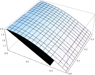
Figure 1: The imagine of $f(x_{1},y_{1})$ and $g(x_{1})$

$f(x_{1},y_{1})$ is the curved surface and $g(x_{1})$ is plane surface. Clearly, $f(x_{1},y_{1})>g(x_{1})$ in definition domain $0<y_{1}\leq\frac{1}{3}$, $0<x_{1}\leq\frac{1}{2}$. Equivalently, $\lambda_{max}^{O}>2d-1$ for any odd $n$ and any number of outcomes $d\geq 2$. Therefore, the quantum bound violates the classical bound.

The case II

For the case $n$ is even, $n\geq 2$. We choose

$$U = |w_{0}\rangle\langle w_{0}|+e^{-i2\pi/dn}|w_{1}\rangle\langle w_{1}|+e^{-i4\pi/dn}|w_{2}\rangle\langle w_{2}|+\cdots$$ (13)

$$+e^{-i(n-2)\pi/dn}|w_{\frac{n-2}{2}}\rangle\langle w_{\frac{n-2}{2}}|+e^{i\pi/d}|w_{\frac{n}{2}}\rangle\langle w_{\frac{n}{2}}|+e^{i(n-2)\pi/dn}|w_{\frac{n+2}{2}}\rangle\langle w_{\frac{n+2}{2}}|$$

$$+\cdots+e^{i4\pi/dn}|w_{n-2}\rangle\langle w_{n-2}|+e^{i2\pi/dn}|w_{n-1}\rangle\langle w_{n-1}|.$$

In this case, the eigenvector corresponding to the maximum eigenvalue of $O$ lies in the subspace when $\lambda=e^{i2\pi/nd}$.

We shall calculate the maximum eigenvalue of the operator

$$R=P_{e^{i2\pi/nd}}\left|0v_{1}^{0}\right>\left<0v_{1}^{0}\right|P_{e^{i2\pi/nd}}+P_{e^{i2\pi/nd}}\left|0v_{1}^{1}\right>\left<0v_{1}^{1}\right|)P_{e^{i2\pi/nd}},$$ (14)

Denote

$$\left|\psi_{1}\right>=P_{e^{i2\pi/nd}}\left|0v_{1}^{0}\right>,\hskip 14.22636pt\left|\psi_{2}\right>=P_{e^{i2\pi/nd}}\left|0v_{1}^{1}\right>,\hskip 14.22636ptM=(\langle\psi_{k}|\psi_{j}\rangle)_{k,j=1}^{2},$$ (15)

then the eigenvalues of $M$ are exactly the ones of $R$. With the help of Wolfram Mathematica 8.0, we get the matrix $M$ has the following form

$$\left(\begin{array}[]{cc}\frac{1}{n}&\frac{1}{n^{2}}(1+X+e^{i\pi/d})\\ \frac{1}{n^{2}}(1+X+e^{-i\pi/d})&\frac{1}{n}\\ \end{array}\right),$$

where $X=\cos\frac{(dn+2-2n)\pi}{2dn}\csc\frac{\pi}{dn}-\cos\frac{(dn-2)\pi}{2dn}\csc\frac{\pi}{dn}$. The maximum eigenvalue of $M$ is $\lambda_{max}^{M}=(n+((1+X+\cos\frac{\pi}{d})^{2}+(\sin\frac{\pi}{d})^{2})^{1/2})/n^{2}$. Thus the maximum eigenvalue $\lambda_{max}^{O}$ of $O$ is

$$\lambda_{max}^{O} = dn\lambda_{max}^{M}$$ (16)

$$= d(n+((1+X+\cos\frac{\pi}{d})^{2}+(\sin\frac{\pi}{d})^{2})^{1/2})/n.$$

Set $y_{2}=\frac{1}{n}$, $x_{2}=\frac{1}{d}$, then $0<y_{2}\leq\frac{1}{2}$, $0<x_{2}\leq\frac{1}{2}$. Define the functions

$$f(x_{2},y_{2}) = 1+y_{2}((1+\widetilde{X}+\cos(x_{2}\pi))^{2}+(\sin x_{2}\pi)^{2})^{\frac{1}{2}},$$ (17)

$$g(x_{2}) = 2-x_{2},$$ (18)

where $\widetilde{X}=\sin(x_{2}\pi-x_{2}y_{2}\pi)\csc(x_{2}y_{2}\pi)-\sin(x_{2}y_{2}\pi)\csc(x_{2}y_{2}\pi)$.

From Wolfram Mathematica 8.0, one obtain the imagine of $f(x_{2},y_{2})$ and $g(x_{2})$ in Figure 2.

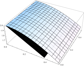
Figure 2: The imagine of $f(x_{2},y_{2})$ and $g(x_{2})$

$f(x_{2},y_{2})$ is the curved surface and $g(x_{2})$ is plane surface. Clearly, in definition domain $0<y_{2}\leq\frac{1}{2}$, $0<x_{2}\leq\frac{1}{2}$, we have $f(x_{2},y_{2})>g(x_{2})$. Equivalently, $\lambda_{max}^{O}>2d-1$ for any odd $n$ and any outcomes $d\geq 2$. Therefore, the quantum bound violates the classical bound.

No matter $n$ is odd or even, the above results can be explained as a nonlocal game.

Figure 3: The structure of nonlocal game

We have that Alice and Bob each receive a bit $s$ and $t$ respectively from a referee, with each bit equally likely to be $0,\ 1,\ \cdots$, or $d-1$. After Alice and Bob perform measurements on their own part respectively, they send measurement results $v_{A}(s)$ and $v_{B}(t)$ back to the referee, $v_{A}(s)$ and $v_{B}(t)$ take values in the set $\{0,1,\cdots,n-1\}$. The structure of the nonlocal game are shown in Figure 3. The winning conditions are listed in Table 1.

s,t	00	11	$\cdots$	(d-1)(d-1)	01	12	$\cdots$	(d-2)(d-1)	(d-1)0
	01	01	$\cdots$	01	01	01	$\cdots$	01	02
Alice,	12	12	$\cdots$	12	12	12	$\cdots$	12	13
Bob	$\cdots$	$\cdots$	$\cdots$	$\cdots$	$\cdots$	$\cdots$	$\cdots$	$\cdots$	$\cdots$
	(d-1)0	(d-1)0	$\cdots$	(d-1)0	(d-1)0	(d-1)0	$\cdots$	(d-1)0	(d-1)1

Table 1: Winning conditions for the nonlocal game($\mathbb{C}^{n}\otimes\mathbb{C}^{n}$)

Specifically, the values of $(s,t)$ are listed on the first row, and the corresponding bit values $v_{A}(s)$ and $v_{B}(t)$ respectively sent by Alice and Bob are listed on the second row. This game is won if the bit values $v_{B}(t)-v_{A}(s)=2\ {\text{m}od}\ d$ when $(s,t)=(d-1,0)$ and if the bit values $v_{B}(t)-v_{A}(s)=1\ {\text{m}od}\ d$ for all other allowed choice of $(s,t)$.

The maximum classical probability of winning this game can be achieved if Alice always returning the bit value $0$ and Bob always returning the bit value $1$. So the maximum classical probability is $\frac{2d-1}{2d}$.

In the quantum strategy, Alice and Bob share the state $\left|\phi\right>$ which is the eigenstate of $O$ corresponding to its maximum eigenvalue $\lambda_{max}^{O}$. If they receive values $s$ and $t$ from the referee respectively, Alice measure $a_{s}$, Bob measure $a_{t}$, and then they send the measurement results to referee. The probability of winning this game is then $\frac{\lambda_{max}^{O}}{2d}$. From Figure 1 and Figure 2, we know that the value of quantum bound is larger than the value of classical bound.

Furthermore, we note that, no matter $n$ is odd or even, the classical bound of Bell inequality Eq.(5) is $2d-1$ which is independent of the choice of $n$. And the quantum bound is decided by both the values of $n$ and $d$.

For $n$ is odd, fix a $x_{1}$, we compute the partial derivative of function $f(x_{1},y_{1})$ with respect to $y_{1}$:

$$\frac{\partial f(x_{1},y_{1})}{\partial y_{1}}=\csc(\pi x_{1}y_{1})\sin(\pi x_{1})-\pi x_{1}y_{1}\cot(\pi x_{1}y_{1})\csc(\pi x_{1}y_{1})\sin(\pi x_{1}).$$ (19)

In the domain $0<y_{1}\leq\frac{1}{3}$, $0<x_{1}\leq\frac{1}{2}$, the trigonometric functions $\csc(\pi x_{1}y_{1})$, $\sin(\pi x_{1})$ and $\cot(\pi x_{1}y_{1})$ are all exceed $0$, so the derivative function $\frac{\partial f(x_{1},y_{1})}{\partial y_{1}}$ always exceed $0$ in the definition domain. Thus the continuous function $f(x_{1},y_{1})$ is a monotonic increasing function for any fixed $x_{1}$. That is to say, the quantum bound $\lambda_{max}^{O}$ is a monotonic decreasing function with respect to $n$ for a fixed $d$, the number of measurements.

Even so, when $d$ is large enough, the quantum bound is independent of the choice of $n$. If each measurement has $3$ outcomes, i.e. $y_{1}=\frac{1}{3}$,

$$f(x_{1},\frac{1}{3}) = 1+\frac{1}{3}+\frac{1}{3}(\sin(x_{1}\pi)\csc\frac{x_{1}\pi}{3}-\sin\frac{x_{1}\pi}{3}\csc\frac{x_{1}\pi}{3})$$ (20)

$$= \frac{2}{3}(2+\cos\frac{2\pi x}{3}).$$

If $n$ is large enough, i.e. $y_{1}\rightarrow 0$, we evaluate the limit value

$$f(x_{1},0) := \lim_{y_{1}\rightarrow 0}f(x_{1},y_{1})$$ (21)

$$= 1+\frac{1}{\pi x}\sin(\pi x).$$

We draw the graphics of functions $f(x_{1},\frac{1}{3})$ and $f(x_{1},0)$ in Figure 4,

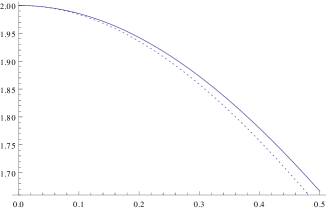
Figure 4: The imagine of $f(x_{1},0)$ and $f(x_{1},\frac{1}{3})$

function $f(x_{1},\frac{1}{3})$ is solid, and function $f(x_{1},0)$ is dotted. From this figure, we see that when $x_{1}$ is near to $0$, $f(x_{1},0)$ approach $f(x_{1},\frac{1}{3})$.

When $n$ is even, we have similar analysis. That is to say, when the number of measurements is large enough, the violation of Bell inequality is determined by the number of measurements $d$ and independent of $n$, the number of outcomes.

III Four partite system

For a four partite system, Alice, Bob, Charlie and Danniel share joint state $\left|\psi\right>$ which are elements of the Hilbert space $\mathbb{C}^{4}\otimes\mathbb{C}^{4}\otimes\mathbb{C}^{4}\otimes\mathbb{C}^{4}$, with each $\mathbb{C}^{4}$ is spanned by the orthonormal basis $\{\left|0\right>,\left|1\right>,\left|2\right>,\left|3\right>\}$. Each of them can take one of two measurements, and for each measurement the possible values for the outcomes are $0$, $1$, $2$ or $3$. Alice’s observable operators are $a_{0}$ and $a_{1}$, Bob’s are $b_{0}$ and $b_{1}$, Charlie’s are $c_{0}$ and $c_{1}$, and Danniel’s are $d_{0}$ and $d_{1}$. The orthonormal basis $\{\left|0\right>,\left|1\right>,\left|2\right>,\left|3\right>\}$ correspond to the observable operators $a_{0}$, $b_{0}$, $c_{0}$ and $d_{0}$, $a_{0}=|1\rangle\langle 1|+2|2\rangle\langle 2|+3|3\rangle\langle 3|$, similarly for $b_{0}$, $c_{0}$ and $d_{0}$. Next we define the second basis.

Since the $4\times 4$ translation operator $T$ is an orthogonal matrix under any orthonormal basis, we have

$$T=|w_{0}\rangle\langle w_{0}|+e^{-i\pi/2}|w_{1}\rangle\langle w_{1}|+e^{i\pi}|w_{2}\rangle\langle w_{2}|+e^{i\pi/2}|w_{3}\rangle\langle w_{3}|,$$ (22)

where

$$|w_{j}\rangle=\frac{1}{2}\sum_{k=0}^{3}e^{i\pi jk/2}\left|j\right>,\hskip 14.22636pt\langle w_{j}|w_{k}\rangle=\delta_{jk}$$ (23)

for any $j,k=0,1,2,3$. Choose operator

$$U=|w_{0}\rangle\langle w_{0}|+e^{-i\pi/4}|w_{1}\rangle\langle w_{1}|+e^{i\pi/2}|w_{2}\rangle\langle w_{2}|+e^{i\pi/4}|w_{3}\rangle\langle w_{3}|,$$ (24)

then the space $\{j\rightarrow U^{j}\mid j=0,1,\cdots,7\}$ is a representation of the cyclic group $\mathbb{Z}_{8}$, the group of integers $\mathbb{Z}$ modulo $8$. We can define the second basis $\{v_{j}=U^{j}\left|j\right>\mid j=0,1,2,3\}$, and this basis corresponds to the observable operators $a_{1}$, $b_{1}$, $c_{1}$ and $d_{1}$, $a_{1}=|v_{1}\rangle\langle v_{1}|+2|v_{2}\rangle\langle v_{2}|+3|v_{3}\rangle\langle v_{3}|$, similarly for $b_{1}$, $c_{1}$ and $d_{1}$. Denote $V=U\otimes U\otimes U\otimes U$, then $\{j\rightarrow V^{j}\mid j=0,1,\cdots,7\}$ is also a representation of the cyclic group $\mathbb{Z}_{8}$. We choose the following six states:

$$\left|000v_{1}\right>,\hskip 14.22636pt\left|0v_{0}v_{0}0\right>,\hskip 14.22636pt\left|0v_{0}0v_{0}\right>,\hskip 14.22636pt\left|v_{0}v_{3}03\right>,\hskip 14.22636pt\left|0v_{1}v_{1}1\right>,\hskip 14.22636pt\left|0v_{2}20\right>,$$ (25)

where state $\left|000v_{1}\right>$ means $\left|0\right>\otimes\left|0\right>\otimes\left|0\right>\otimes\left|v_{1}\right>$. Each of these six states in (25) has an orbit with $8$ elements under the action of $\{V^{j}|j=0,1,\cdots,7\}$, and the six orbits are distinct. The set of all states in the six orbits leads to a violation of Bell inequality. The specific analysis is given as follows.

For each state in the six orbits, it corresponds to a particular choice of measurements and the corresponding measurement results. For example, for the state $\left|000v_{1}\right>$, it corresponds to the fact that Alice measuring $a_{0}$ and obtaining $0$, Bob measuring $b_{0}$ and obtaining $0$, Charlie measuring $c_{0}$ and obtaining $0$, Danniel measuring $d_{1}$ and obtaining $1$.

From local realistic theory, the sum of these $48$ events give a Bell inequality, it reads

$$\footnotesize{\begin{split}&\sum_{j=0}^{3}P(a_{0}=b_{0}=c_{0}=j,d_{1}=j\oplus 1)+\sum_{j=0}^{3}P(a_{1}=b_{1}=c_{1}=j,d_{0}=j\oplus 2)\\ &+\sum_{j=0}^{3}P(a_{0}=b_{1}=c_{1}=d_{0}=j)+\sum_{j=0}^{3}P(a_{1}=d_{1}=j,b_{0}=c_{0}=j\oplus 1)\\ &+\sum_{j=0}^{3}P(a_{0}=b_{1}=c_{0}=d_{1}=j)+\sum_{j=0}^{3}P(a_{1}=c_{1}=j,b_{0}=d_{0}=j\oplus 1)\\ &+\sum_{j=0}^{3}P(a_{1}=c_{0}=j,b_{1}=d_{0}=j\oplus 3)+\sum_{j=0}^{3}P(a_{0}=j,b_{0}=c_{1}=j\oplus 3,d_{1}=j\oplus 2)\\ &+\sum_{j=0}^{3}P(a_{0}=d_{0}=j,b_{1}=c_{1}=j\oplus 1)+\sum_{j=0}^{3}P(a_{1}=d_{1}=j,b_{0}=c_{0}=j\oplus 1)\\ &+\sum_{j=0}^{3}P(a_{0}=d_{0}=j,b_{1}=c_{0}=j\oplus 2)+\sum_{j=0}^{3}P(a_{1}=d_{1}=j,b_{0}=j\oplus 3,c_{1}=j\oplus 2)\leq 2,\end{split}}$$ (26)

where $\oplus$ means the addition modulo $4$, $P(a_{0}=b_{0}=c_{0}=j,d_{1}=j\oplus 1)$ means the probability of the event when Alice, Bob and Charlie take measure $a_{0}$, $b_{0}$ and $c_{0}$ respectively and obtain the same value $j$, Danniel take measure $d_{1}$ and obtain value $j\oplus 1$. But in quantum bound can attain the value $2.021$.

In order to maximize the sum of probabilities corresponding to these $48$ states in quantum mechanics, we need to find a state $\left|\phi\right>$, such that the expectation value $\langle\phi|O|\phi\rangle$ is maximum, where

$$O=\sum_{j=0}^{7}V^{j}L(V^{{\dagger}})^{j},$$ (27)

and

$$\begin{split}&L=\left|000v_{1}\right>\left<000v_{1}\right|+\left|0v_{0}v_{0}0\right>\left<0v_{0}v_{0}0\right|+\left|0v_{0}0v_{0}\right>\left<0v_{0}0v_{0}\right|+\\ &\qquad\left|v_{0}v_{3}03\right>\left<v_{0}v_{3}03\right|+\left|0v_{1}v_{1}1\right>\left<0v_{1}v_{1}1\right|+\left|0v_{2}20\right>\left<0v_{2}20\right|.\end{split}$$ (28)

The maximum value of $\langle\phi|O|\phi\rangle$ occurs when $\left|\phi\right>$ is the eigenstate of $O$ corresponding to its maximum eigenvalue. So the question is reduced to how to calculate the maximum eigenvalue of $O$.

Note that the eigenstates of $V$ are states of the form $\left|w_{k}w_{l}w_{m}w_{n}\right>$ for $k,\ l,\ m,\ n=0,\ 1,\ 2,\ 3$, and the eigenvalues are $\pm 1$, $e^{\pm i\pi/4}$, $e^{\pm i\pi/2}$ and $e^{\pm 3i\pi/4}$. The spectral decomposition $V=\sum_{\lambda}\lambda P_{\lambda}$, leads to a simplification of $O$, $O=8\sum_{\lambda}P_{\lambda}LP_{\lambda}.$ The eigenvector corresponding to the maximum eigenvalue of $O$ lies in the subspace when $V$ has eigenvalue $e^{i\pi/2}$. Set

$$\left|\psi_{1}\right>=P_{e^{i\pi/2}}\left|000v_{1}\right>,\hskip 14.22636pt\left|\psi_{2}\right>=P_{e^{i\pi/2}}\left|0v_{0}v_{0}0\right>,\hskip 14.22636pt\left|\psi_{3}\right>=P_{e^{i\pi/2}}\left|0v_{0}0v_{0}\right>,$$

$$\left|\psi_{4}\right>=P_{e^{i\pi/2}}\left|v_{0}v_{3}03\right>,\hskip 14.22636pt\left|\psi_{5}\right>=P_{e^{i\pi/2}}\left|0v_{1}v_{1}1\right>,\hskip 14.22636pt\left|\psi_{6}\right>=P_{e^{i\pi/2}}\left|0v_{2}20\right>,$$

and $R=P_{e^{i\pi/2}}LP_{e^{i\pi/2}}$, then the operator can be written as,

$$R=\sum_{j=1}^{6}\left|\psi_{j}\right>\left<\psi_{j}\right|.$$ (29)

Note that the eigenvectors of $R$ can be expressed as $\sum_{j=1}^{6}x_{j}\left|\psi_{j}\right>$, then there exists eigenvalue $\mu$ such that $\sum_{k=1}^{6}\left|\psi_{k}\right>\left<\psi_{k}\right|\sum_{j=1}^{6}x_{j}\left|\psi_{j}\right>=\mu\sum_{j=1}^{6}x_{j}\left|\psi_{j}\right>$. Rewrite the eigenvalue equation, it becomes

$$\sum_{j=1}^{6}x_{j}\langle\psi_{k}|\psi_{j}\rangle\sum_{k=1}^{6}\left|\psi_{k}\right>=\mu\sum_{k=1}^{6}x_{k}\left|\psi_{k}\right>.$$ (30)

Equivalently, for any $k=1,2,\cdots,6$, we have $\sum_{j=1}^{6}x_{j}\langle\psi_{k}|\psi_{j}\rangle=\mu x_{k}$. Denote the matrix $M=(\langle\psi_{k}|\psi_{j}\rangle)_{k,j=1}^{6}$, then the eigenvalues of $M$ are exactly the ones of $R$. With the help of Wolfram Mathematica 8.0, we quickly obtain the matrix $256M$ as the following form

$$\tiny{\left(\begin{array}[]{cccccc}\vskip 6.0pt plus 2.0pt minus 2.0pt44&-2-\sqrt{2}+i\sqrt{2}&-2-\sqrt{2}+i\sqrt{2}&-\sqrt{2}-i(2+\sqrt{2})&4-3\sqrt{2}+i(\sqrt{2}-2)&4-4i\\ \vskip 6.0pt plus 2.0pt minus 2.0pt-2-\sqrt{2}-i\sqrt{2}&44&8+4\sqrt{2}&i4\sqrt{2}&8i&-\sqrt{2}+i(2-\sqrt{2})\\ \vskip 6.0pt plus 2.0pt minus 2.0pt-2-\sqrt{2}-i\sqrt{2}&8+4\sqrt{2}&44&0&0&-\sqrt{2}+i(2-\sqrt{2})\\ \vskip 6.0pt plus 2.0pt minus 2.0pt-\sqrt{2}+i(2+\sqrt{2})&-i4\sqrt{2}&0&44&0&-2+\sqrt{2}-i\sqrt{2}\\ \vskip 6.0pt plus 2.0pt minus 2.0pt4-3\sqrt{2}-i(\sqrt{2}-2)&-8i&0&0&44&2+\sqrt{2}+i(4+3\sqrt{2})\\ 4+4i&-\sqrt{2}-i(2-\sqrt{2})&-\sqrt{2}-i(2-\sqrt{2})&-2+\sqrt{2}+i\sqrt{2}&2+\sqrt{2}-i(4+3\sqrt{2})&44\\ \end{array}\right),}$$

and obtain the numerical approximate value of the maximum eigenvalue of $M$ is $64.667/256$. Thus the maximum eigenvalue of $O$ is $8\times\frac{64.667}{256}\approx 2.021>2$. So we get a violation.

The above results can be explained as a nonlocal game. The bits $s$, $t$, $u$ and $v$ are sent to Alice, Bob, Charlie and Danniel respectively from the same referee, take value $0$ or $1$ with equally likely possibility. Alice take measure $a_{s}$ on her part, Bob take measure $b_{t}$ on his part, Charlie take measure $c_{u}$ on her part, Danniel take measure $d_{v}$ on his part. Then they each send a bit value $v_{A}(s)$, $v_{B}(t)$, $v_{C}(u)$ and $v_{D}(v)$ back to the referee, the bit values take values in the set $\{0,\ 1,\ 2,\ 3\}$. The winning conditions are listed in Table 2.

s,t,u,v	Alice, Bob, Charlie, Danniel
0001	0001, 1112, 2223, 3330
1110	0002, 1113, 2220, 3331
0110	0000, 1111, 2222, 3333
1001	0110, 1221, 2332, 3003
0101	0000, 1111, 2222, 3333
1010	0101, 1212, 2323, 3030

s,t,u,v	Alice, Bob, Charlie, Danniel
1100	0303, 1010, 2121, 3232
0011	0332, 1003, 2110, 3221
0110	0111, 1222, 2333, 3000
1001	0221, 1332, 2003, 3110
0100	0220, 1331, 2002, 3113
1011	0320, 1031, 2102, 3213

Table 2: Winning conditions for the nonlocal game(4parties)

Specifically, the values of $(s,t,u,v)$ are listed on the left, and the corresponding outcomes $v_{A}(s)$, $v_{B}(t)$, $v_{C}(u)$ and $v_{D}(v)$ sent by Alice, Bob, Charlie and Danniel are listed on the right. The maximum classical probability of winning this game can be achieved when the outcomes $v_{A}(s)$, $v_{B}(t)$, $v_{C}(u)$ and $v_{D}(v)$ take same value, $(s,t,u,v)$ take value $(0110)$ or $(0110)$. So the maximum classical probability is $\frac{2}{12}\approx 0.1667$.

In the quantum strategy, Alice, Bob, Charlie and Danniel share the state $\phi$ which is the eigenstate of $O$ corresponding to its maximum eigenvalue $2.021$. If they receive values $s$, $t$, $u$ and $v$ from the referee respectively, Alice measure $a_{s}$, Bob measure $a_{t}$, Charlie measure $a_{u}$ and Danniel measure $a_{v}$, then they send the measurement results to referee. With this strategy, the probability of winning this game is $0.1684$.

IV Three partite system

Alice, Bob and Charlie make measurements, each party make one of $2$ possible measurements, and each measurement has $4$ outcomes. As above, the orthonormal basis $\{\left|0\right>,\left|1\right>,\left|2\right>,\left|3\right>\}$ correspond to the observables $a_{0}$, $b_{0}$ and $c_{0}$, $a_{0}=|1\rangle\langle 1|+2|2\rangle\langle 2|+3|3\rangle\langle 3|$, similarly for $b_{0}$ and $c_{0}$. The orthonormal basis $\{\left|v_{0}\right>,\left|v_{1}\right>,\left|v_{2}\right>,\left|v_{3}\right>\}$ correspond to the observables $a_{1}$, $b_{1}$ and $c_{1}$, $a_{1}=|v_{1}\rangle\langle v_{1}|+2|v_{2}\rangle\langle v_{2}|+3|v_{3}\rangle\langle v_{3}|$, similarly for $b_{1}$ and $c_{1}$.

We restrict the six orbits in Eq.(25) to three partite system by forgetting the last party, and guarantee the bound of probabilities from local realistic theory invariant. We get $4$ orbits in $\mathbb{C}^{4}\otimes\mathbb{C}^{4}\otimes\mathbb{C}^{4}$, which will get a violation of Bell inequality. The representative elements of the $4$ orbits are:

$$\left|0v_{0}v_{0}\right>,\hskip 14.22636pt\left|v_{0}v_{3}0\right>,\hskip 14.22636pt\left|0v_{1}v_{1}\right>,\hskip 14.22636pt\left|0v_{2}2\right>.$$ (31)

Each of the four states in Eq.(31) has an orbit with $8$ elements under the action of $\{U^{j}\otimes U^{j}\otimes U^{j}|j=0,1,\cdots,7\}$, and the four orbits are distinct. From local realistic theory, the sum of these $32$ states give a Bell inequality. It reads

$$\footnotesize{\begin{split}&\sum_{j=0}^{3}P(a_{0}=b_{1}=c_{1}=j)+\sum_{j=0}^{3}P(a_{1}=j,b_{0}=c_{0}=j\oplus 1)\\ &+\sum_{j=0}^{3}P(a_{1}=c_{0}=j,b_{1}=j\oplus 3)+\sum_{j=0}^{3}P(a_{0}=j,b_{0}=c_{1}=j\oplus 3)\\ &+\sum_{j=0}^{3}P(a_{0}=j,b_{1}=c_{1}=j\oplus 1)+\sum_{j=0}^{3}P(a_{1}=j,b_{0}=c_{0}=j\oplus 2)\\ &+\sum_{j=0}^{3}P(a_{0}=j,b_{1}=c_{0}=j\oplus 2)+\sum_{j=0}^{3}P(a_{1}=j,b_{0}=j\oplus 3,c_{1}=j\oplus 2)\leq 2,\end{split}}$$ (32)

where $\oplus$ means the addition modulo $4$. But the quantum bound of the sum of these probabilities can attain the value $2.075$.

Similarly, we need to find a special state $\left|\phi\right>$, such that the expectation value $\langle\phi|O|\phi\rangle$ is maximum, where

$$O=\sum_{j=0}^{7}(U\otimes U\otimes U)^{j}L(U^{{\dagger}}\otimes U^{{\dagger}}\otimes U^{{\dagger}})^{j},$$ (33)

and

$$L=\left|0v_{0}v_{0}\right>\left<0v_{0}v_{0}\right|+\left|v_{0}v_{3}0\right>\left<v_{0}v_{3}\right|+\left|0v_{1}v_{1}\right>\left<0v_{1}v_{1}\right|+\left|0v_{2}2\right>\left<0v_{2}2\right|.$$ (34)

Note that the eigenstates of $U\otimes U\otimes U$ are states of the form $\left|w_{k}w_{m}w_{n}\right>$ for $k,\ m,\ n=0,\ 1,\ 2,\ 3$, and the eigenvalues are $\pm 1$, $e^{\pm i\pi/4}$, $e^{\pm i\pi/2}$ and $e^{\pm 3i\pi/4}$. For the spectral decomposition of $U$, $U\otimes U\otimes U=\sum_{\lambda}\lambda P_{\lambda}$, the operator $O$ can be simplified as

$$O=8\sum_{\lambda}P_{\lambda}LP_{\lambda}.$$ (35)

The eigenvector corresponding to the maximum eigenvalue of $O$ lies in the subspace when $U\otimes U\otimes U$ has eigenvalue $e^{i\pi/2}$. Set

$$\left|\psi_{1}\right>=P_{e^{i\pi/2}}\left|0v_{0}v_{0}\right>,\hskip 14.22636pt\left|\psi_{2}\right>=P_{e^{i\pi/2}}\left|v_{0}v_{3}0\right>,$$

$$\left|\psi_{3}\right>=P_{e^{i\pi/2}}\left|0v_{1}v_{1}\right>,\hskip 14.22636pt\left|\psi_{4}\right>=P_{e^{i\pi/2}}\left|0v_{2}2\right>.$$ (36)

Denote the operator $P_{e^{i\pi/2}}LP_{e^{i\pi/2}}$ by $R$, then $R$ can be write as $R=\sum_{j=1}^{4}\left|\psi_{j}\right>\left<\psi_{j}\right|.$ Suppose that the eigenvectors of $R$ corresponding to eigenvalue $\mu$ is $\sum_{j=1}^{4}x_{j}\left|\psi_{j}\right>$, then the eigenvalue equation can be rewritten as

$$\sum_{j=1}^{4}x_{j}\langle\psi_{k}|\psi_{j}\rangle\sum_{k=1}^{4}\left|\psi_{k}\right>=\mu\sum_{k=1}^{4}x_{k}\left|\psi_{k}\right>.$$ (37)

Denote the matrix $M=(\langle\psi_{k}|\psi_{j}\rangle)_{k,j=1}^{4}$. The eigenvalues of $M$ are exactly the ones of $R$. With the help of Mathematics, we obtain the matrix $M$ as the following form

$$\small{\frac{1}{64}\left(\begin{array}[]{cccc}12&i\sqrt{2}&2i&1+i\\ -i\sqrt{2}&12&-1-i&\sqrt{2}\\ -2i&-1+i&12&2i+i\sqrt{2}\\ 1-i&\sqrt{2}&-2i-i\sqrt{2}&12\\ \end{array}\right),}$$

and obtain the numerical approximate value of the maximum eigenvalue of $M$ is $16.597/64$. Thus the maximum eigenvalue of $O$ is $8\times\frac{16.597}{64}\approx 2.075>2$.

This results can also be phrased as a nonlocal game. Alice, Bob and Charlie each receive a bit $s$, $t$ and $u$ respectively from same referee. $s$, $t$ and $u$ take value $0$ or $1$ with equally likely possibility. Then Alice make measurement $a_{s}$, Bob make measurement $b_{t}$ and Charlie make measurement $c_{u}$. They return the measurement results $v_{A}(s)$, $v_{B}(t)$ and $v_{C}(u)$ back to the referee respectively, the outcomes take values in the set $\{0,\ 1,\ 2,\ 3\}$. The winning conditions are listed in Table 3.

s,t,u	Alice, Bob, Charlie
011	000, 111, 222, 333
100	011, 122, 233, 300
110	030, 101, 212, 323
001	033, 100, 211, 322

s,t,u	Alice, Bob, Charlie
011	011, 122, 233, 300
100	022, 133, 200, 311
010	022, 133, 200, 311
101	032, 103, 210, 321

Table 3: Winning conditions for the nonlocal game(3parties)

Specifically, the values of $(s,t,u)$ are listed on the left, and the corresponding measurement results $v_{A}(s)$, $v_{B}(t)$ and $v_{C}(u)$ sent by Alice, Bob and Charlie are listed on the right. Note that, the states listed in (31) is obtained by the states in (25) by forgetting the last bit and an additional condition. The Table 3 is obtained by deleting the first two rows and the last two rows in the left table of Table 2, and forgetting the last bit values. The maximum classical probability of winning this game is $\frac{2}{8}\approx 0.25$.

In the quantum strategy, Alice, Bob and Charlie share the state $\phi$ which is the eigenstate of $O$ corresponding to its maximum eigenvalue $2.075$. If they receive values $s$, $t$ and $u$ from the referee respectively, then Alice measure $a_{s}$, Bob measure $a_{t}$, Charlie measure $a_{u}$, and they send the measurement results to referee. With this strategy, the probability of winning this game is $0.2594$.

Acknowledgement

This work is supported by NSFC 11571119 and NSFC 11475178.

References

[1] J.S. Bell, Physica1, 195 (1964)
[2] J.F. Clauser, M.A. Horne, A. Shimony, R.A. Holt, Phys. Rev. Lett.23, 880 (1969)
[3] J.F. Clauser, M.A. Horne, Phys. Rev. D10, 526 (1974)
[4] D. Kaszlikowski, P. Gnacinski, M. Zukowski, W. Miklaszewski, A. Zeilinger, Phys. Rev. Lett.85, 4418 (2000)