Evolution of the magnetic field in neutron stars

Abstract

We propose a general method to self-consistently study the quasistationary evolution of the magnetic field in the cores of neutron stars. The traditional approach to this problem is critically revised. Our results are illustrated by calculation of the typical timescales for the magnetic field dissipation as functions of temperature and the magnetic field strength.

I Introduction

Magnetic field plays a crucial role in the evolution of neutron stars (NSs). Quite possibly, it serves as a most important unifying agent relating and explaining the observational properties of many diverse classes of NSs (e.g., rotation-powered pulsars, magnetars, isolated neutron stars etc.) Kaspi (2010); Viganò et al. (2013). If this is true, non-accreting NSs from different classes differ mainly in their age and the magnetic field at birth. To extract as much information from observations as possible one, therefore, needs to be able to adequately model the long-term magneto-thermal evolution of NSs with different initial magnetic field configurations. Clearly, this is a very complex theoretical problem, which has not been fully solved yet (but see, e.g., Refs. Haensel et al. (1990); Urpin and Shalybkov (1995); Page et al. (2000); Arras et al. (2004); Aguilera et al. (2008); Pons et al. (2009); Viganò et al. (2013)).

One of the aspects of this problem is the way magnetic field evolves and dissipates in the internal layers of NSs. Up to now a substantial body of research on this subject has been concentrated on the crust (see, e.g., Refs. Jones (1988); Shalybkov and Urpin (1997); Rheinhardt and Geppert (2002); Hollerbach and Rüdiger (2004); Gourgouliatos et al. (2013); Gourgouliatos and Cumming (2014); Gourgouliatos et al. (2016) and references therein). Because the ionic lattice of the crust is immobile, the magnetic field there evolves exclusively through the Ohmic decay and Hall drift. The case of the core is much more complex, since there we have at least three particle species (neutrons, protons, and electrons) that can move one relative to another, so the diffusion effects come into play in addition to the two processes active in the crust.

Evolution of the magnetic field in the core has been studied, under various simplifying assumptions, e.g., in Refs. Baym et al. (1969); Haensel et al. (1990); Pethick (1992); Urpin and Ray (1994); Urpin and Shalybkov (1995); Thompson and Duncan (1996); Urpin and Shalybkov (1999); Konenkov and Geppert (2000, 2001); Arras et al. (2004); Braithwaite and Spruit (2006); Hoyos et al. (2008); Dall’Osso et al. (2009); Hoyos et al. (2010); Ho (2011); Dall’Osso et al. (2012); Graber et al. (2015); Elfritz et al. (2016); Beloborodov and Li (2016). However, self-consistent analysis of this problem has never been attempted. To perform such an analysis one needs to solve (iterate in time) the Faraday induction equation, $\partial{\boldsymbol{B}}/\partial t=-c\,{\boldsymbol{\nabla}}\times{\boldsymbol{E}}$, where the electric field ${\boldsymbol{E}}$ depends itself on the magnetic field ${\boldsymbol{B}}$, diffusion currents, perturbed chemical potentials etc. A primary problem, therefore, consists in finding ${\boldsymbol{E}}$ (and other parameters in the system) for a given quasistationary magnetic field configuration. This problem has been addressed in a number of papers Shalybkov and Urpin (1995); Thompson and Duncan (1996); Hoyos et al. (2008); Reisenegger (2009); Hoyos et al. (2010); Glampedakis et al. (2011a); Beloborodov and Li (2016); Passamonti et al. (2017) starting from the work of Goldreich and Reisenegger Goldreich and Reisenegger (1992). Unfortunately, the validity of some approximations made in these references remains unclear. Here we reconsider this problem. Namely, we propose a method of obtaining the self-consistent solutions describing quasi-stationary evolution of the magnetic field in NSs. Our results indicate that the conventional approach of Refs. Goldreich and Reisenegger (1992); Thompson and Duncan (1996); Hoyos et al. (2008); Reisenegger (2009); Hoyos et al. (2010); Glampedakis et al. (2011a); Beloborodov and Li (2016); Passamonti et al. (2017) may not be adequate.

The paper is organised as follows. In Sec. II we formulate dynamic equations describing a magnetized mixture of nonsuperfluid/nonsuperconducting particles (e.g., neutrons, protons, and electrons in the NS core). In Sec. III we propose a general scheme, allowing us to determine all the necessary ingredients to calculate the electric field in an NS with a specified (axisymmetric) magnetic field configuration. In Sec. IV we discuss how the proposed scheme should be modified to account for muons (or other particle species), non-axisymmetric fields, and nucleon superfluidity/superconductivity. In Sec. V we derive expressions for the dissipation rate of the magnetic energy in NS cores. In Sec. VI the results of the preceding sections are illustrated by calculation (and comparison) of the magnetic field decay rates due to different dissipation processes: Ohmic decay, non-equilibrium beta-reactions, and ambipolar diffusion. Finally, Sec. VII contains our conclusions and summary of results.

II General equations

We consider a nonsuperfluid and nonsuperconducting matter composed of various (possibly, charged) particle species $\alpha$. The effects of General relativity are neglected for clarity, but the equation of state is assumed to be fully relativistic.We also neglect thermal forces and the effects of temperature on the equation of state. Then the equations that govern evolution of the system can be written as (see, e.g., Refs. Iakovlev and Shalybkov (1991); Goldreich and Reisenegger (1992); Passamonti et al. (2017))

$$\frac{\partial}{\partial t}\left(\frac{\mu_{\alpha}n_{\alpha}}{c^{2}}\,{\boldsymbol{u}}_{\alpha}\right)+\nabla_{k}\left(\frac{\mu_{\alpha}n_{\alpha}}{c^{2}}u_{(\alpha)i}u_{(\alpha)k}\right)$$

$$=\frac{\mu_{\alpha}\Delta\Gamma_{\alpha}}{c^{2}}{\boldsymbol{u}}_{\alpha}+e_{\alpha}n_{\alpha}\left({\boldsymbol{E}}+\frac{1}{c}\left[{\boldsymbol{u}}_{\alpha}\times{\boldsymbol{B}}\right]\right)-n_{\alpha}{\boldsymbol{\nabla}}\mu_{\alpha}-\frac{\mu_{\alpha}n_{\alpha}}{c^{2}}\,{\boldsymbol{\nabla}}\phi-\sum_{\beta\neq\alpha}J_{\alpha\beta}({\boldsymbol{u}}_{\alpha}-{\boldsymbol{u}}_{\beta}),$$ (1)

$$\frac{\partial n_{\alpha}}{\partial t}+{\rm div}(n_{\alpha}\boldsymbol{u}_{\alpha})=\Delta\Gamma_{\alpha},$$ (2)

$$\Delta\phi=\frac{4\pi G}{c^{2}}\,(P+\varepsilon),$$ (3)

$$\frac{\partial{\boldsymbol{B}}}{\partial t}=-c\,{\boldsymbol{\nabla}}\times{\boldsymbol{E}},$$ (4)

$${\boldsymbol{\nabla}}\times{\boldsymbol{B}}=\frac{4\pi}{c}\,{\boldsymbol{j}},$$ (5)

$$\sum_{\alpha}e_{\alpha}n_{\alpha}=0.$$ (6)

The first of these equations is the momentum conservation equation for each particle species $\alpha$; the subscripts $i$ and $k$ there are the spatial indices. The physical meaning of other equations is clear. In these equations $c$ and $G$ are the speed of light and gravitational constant, respectively; $\mu_{\alpha}$ and $n_{\alpha}$ are the relativistic chemical potential and number density for particle species $\alpha$; $\phi$ is the gravitational potential; $P$ and $\varepsilon$ are the total pressure and energy density, respectively,

$$P=-\varepsilon+\sum_{\alpha}\mu_{\alpha}n_{\alpha},$$ (7)

$$dP=\sum_{\alpha}n_{\alpha}d\mu_{\alpha};$$ (8)

${\boldsymbol{u}}_{\alpha}\equiv[u_{(\alpha)1},\,u_{(\alpha)2},\,u_{(\alpha)3}]$ is the velocity of particles $\alpha$; $J_{\alpha\beta}=J_{\beta\alpha}$ is the quantity defined (and calculated) in Ref. Iakovlev and Shalybkov (1991) and related to the effective relaxation time $\tau_{\alpha\beta}$ for scattering of particles $\alpha$ on particles $\beta$ by the formula Iakovlev and Shalybkov (1991): $\tau_{\alpha\beta}=n_{\alpha}\mu_{\alpha}/(c^{2}J_{\alpha\beta})$; the terms in Eq. (1), which depend on $J_{\alpha\beta}$, represent the friction forces. Further, ${\boldsymbol{E}}$ and ${\boldsymbol{B}}$ are the electric and magnetic fields; $e_{\alpha}$ is the electric charge of particle species $\alpha$; and

$${\boldsymbol{j}}=\sum_{\alpha}e_{\alpha}n_{\alpha}{\boldsymbol{u}}_{\alpha}$$ (9)

is the electric current density [note that ${\rm div}\,{\boldsymbol{j}}=0$ in view of Eq. (5)]. Finally, the source $\Delta\Gamma_{\alpha}$ in the continuity equation (2) appears due to non-equilibrium processes of particle mutual transformations (e.g., non-equilibrium Urca processes Yakovlev et al. (2001)). Note that we neglected the displacement current in Eq. (5) and assumed the quasineutrality condition (6), which is a perfect approximation for slow processes we are interested in (see, e.g., Ref. Landau and Lifshitz (1960) for justification of this assumption).

The system of equations (1)–(6) is rather general but it is too complex. It can be further simplified if the hydrodynamic description of the system is justified, i.e. if the inter-particle collisions are so frequent, that $\tau_{\alpha\beta}\ll\tau_{\rm B}$ (see Sec. VI), where $\tau_{\rm B}$ is a typical timescale of the problem (in our case, it is the magnetic field evolution timescale). Then the velocities ${\boldsymbol{u}}_{\alpha}$ of different particle species $\alpha$ are very close to one another (e.g., Ref. Braginskii (1965)), so that it is convenient to introduce the macroscopic velocity of the flow ${\boldsymbol{U}}$ according to Iakovlev and Shalybkov (1991)

$${\boldsymbol{U}}\sum_{\alpha}\mu_{\alpha}n_{\alpha}\equiv\sum_{\alpha}\mu_{\alpha}n_{\alpha}\,{\boldsymbol{u}}_{\alpha},$$ (10)

and replace Eq. (1) with

$$\frac{\partial}{\partial t}\left(\frac{\mu_{\alpha}n_{\alpha}}{c^{2}}\,{\boldsymbol{U}}\right)+\nabla_{k}\left(\frac{\mu_{\alpha}n_{\alpha}}{c^{2}}U_{i}U_{k}\right)$$

$$=\frac{\mu_{\alpha}\Delta\Gamma_{\alpha}}{c^{2}}{\boldsymbol{U}}+e_{\alpha}n_{\alpha}\left({\boldsymbol{E}}+\frac{1}{c}\left[{\boldsymbol{u}}_{\alpha}\times{\boldsymbol{B}}\right]\right)-n_{\alpha}{\boldsymbol{\nabla}}\mu_{\alpha}-\frac{\mu_{\alpha}n_{\alpha}}{c^{2}}\,{\boldsymbol{\nabla}}\phi-\sum_{\beta\neq\alpha}J_{\alpha\beta}\,({\boldsymbol{u}}_{\alpha}-{\boldsymbol{u}}_{\beta}).$$ (11)

To obtain this equation we neglected a number of small terms in Eq. (1), making use of the fact that $\tau_{\rm B}\gg\tau_{\alpha\beta}=n_{\alpha}\mu_{\alpha}/(c^{2}J_{\alpha\beta})$ (see, e.g., Ref. Braginskii (1965) for a similar discussion). For example, we neglected the terms $\partial/\partial t[\mu_{\alpha}n_{\alpha}({\boldsymbol{u}}_{\alpha}-{\boldsymbol{U}})/c^{2}]\sim\mu_{\alpha}n_{\alpha}({\boldsymbol{u}}_{\alpha}-{\boldsymbol{U}})/(\tau_{\rm B}c^{2})$ in comparison to the terms $\sum_{\beta\neq\alpha}J_{\alpha\beta}({\boldsymbol{u}}_{\alpha}-{\boldsymbol{u}}_{\beta})=\sum_{\beta\neq\alpha}\mu_{\alpha}n_{\alpha}/(c^{2}\tau_{\alpha\beta})\,({\boldsymbol{u}}_{\alpha}-{\boldsymbol{u}}_{\beta})$. We also replaced ${\boldsymbol{u}}_{\alpha}$ with ${\boldsymbol{U}}$ in (already) small dissipative term $\mu_{\alpha}\Delta\Gamma_{\alpha}{\boldsymbol{u}}_{\alpha}/c^{2}$, appearing due to the action of weak processes of particle mutual transformations.

Summing up Eq. (11) over all particle species and neglecting the term, quadratically small in the deviation from chemical equilibrium, one obtains the standard force balance equation for the system as a whole,

$$\frac{\partial}{\partial t}\left[\frac{(P+\varepsilon)}{c^{2}}\,{\boldsymbol{U}}\right]+\nabla_{k}\left[\frac{(P+\varepsilon)}{c^{2}}U_{i}U_{k}\right]=\frac{1}{c}\left[{\boldsymbol{j}}\times{\boldsymbol{B}}\right]-{\boldsymbol{\nabla}}P-\frac{(P+\varepsilon)}{c^{2}}\,{\boldsymbol{\nabla}}\phi.$$ (12)

III The problem of magnetic field evolution in the NS cores: General scheme of the solution

The equations of the previous section describe an arbitrary mixture (plasma) of charged particles, provided that they are nonsuperfluid and nonsuperconducting. Here we apply them to the particular case of NS matter composed of neutrons ($n$), protons ($p$), and electrons ($e$) [$npe$-matter]. Extension of these results to more complex NS core compositions (e.g., $npe$-matter with an admixture of muons) is straightforward and is discussed in Sec. IV, where we also consider the effects of non-axisymmetric magnetic field and nucleon superfluidity/superconductivity.

III.1 Our approximations and further simplifications

Assume that the star is nonrotating and spherically symmetric in the absence of the magnetic field. It is in hydrostatic, diffusion, and beta-equilibrium; all particle currents are absent. Then we slightly perturb the system by creating some small currents. They generate the magnetic field, which we, for simplicity, take axisymmetric, ${\boldsymbol{B}}={\boldsymbol{B}}(r,\,\theta)$ (non-axisymmetric case is briefly analysed in Sec. IV.2).

After perturbation is applied, the system starts to evolve to equilibrium through particle diffusion and beta-processes. This process is accompanied by the magnetic field dissipation. A typical timescale for reaching the equilibrium (i.e., the timescale of magnetic field decay) is very large (see below), so that the system evolves through a set of quasistationary states, which means that one can neglect time derivatives in Eqs. (1), (2), (11), (12) of the previous section [and, in addition, ignore the quadratically small velocity-dependent terms, in particular, the term depending on $U_{i}U_{k}$ in Eq. (12)]. We follow here the ideas of Ref. Goldreich and Reisenegger (1992).

Let us demonstrate, for example, that the time derivative in the continuity equation (2) can be omitted. Below the perturbation of a quantity $A$ will be denoted as $\delta A$. From Eqs. (5) and (12) it follows that the perturbation of the pressure $P$ by the magnetic field is $\delta P\sim B^{2}$. Correspondingly, $\delta n_{\alpha}\sim n_{\alpha}B^{2}/P$ and $\partial n_{\alpha}/\partial t\sim n_{\alpha}B^{2}/(P\tau_{\rm B})$. The magnetic evolution timescale $\tau_{\rm B}$ is given by [see Eq. (4)]: $B/\tau_{\rm B}\sim cE/R\sim u_{\alpha}B/R$, hence $\tau_{\rm B}\sim R/u_{\alpha}$ (here $R$ is the typical lengthscale; to obtain $\tau_{\rm B}$ we estimated $E$ as: $E\sim u_{\alpha}B/c$). Now we can write $\partial n_{\alpha}/\partial t\sim n_{\alpha}B^{2}/(P\tau_{\rm B})\sim n_{\alpha}u_{\alpha}B^{2}/(PR)$, while $|{\rm div}(n_{\alpha}{\boldsymbol{u}}_{\alpha})|\sim n_{\alpha}u_{\alpha}/R$. Comparing these terms, it is easy to see that $\partial n_{\alpha}/\partial t$ drops out from the continuity equation written to leading order in $B^{2}/P$.

Accounting for the approximations listed above, Eq. (12) can be represented as [we make use of Eqs. (7) and (8)]

$$\sum_{\alpha}n_{\alpha}{\boldsymbol{\nabla}}\mu_{\alpha}^{\infty}=\frac{1}{c}\left[{\boldsymbol{j}}\times{\boldsymbol{B}}\right],$$ (13)

where we introduced the redshifted chemical potentials, $\mu_{\alpha}^{\infty}=\mu_{\alpha}e^{\phi/c^{2}}$; in the weak-field approximation ${\boldsymbol{\nabla}}\mu_{\alpha}^{\infty}\approx{\boldsymbol{\nabla}}\mu_{\alpha}+(\mu_{\alpha}/c^{2})\,{\boldsymbol{\nabla}}\phi$. Using the quasineutrality condition (6) and the definitions $\Delta\mu_{e}\equiv\mu_{p}+\mu_{e}-\mu_{n}$ and $n_{b}=n_{p}+n_{n}$, Eq. (13) can be rewritten as

$$n_{e}{\boldsymbol{\nabla}}\Delta\mu_{e}^{\infty}+n_{b}{\boldsymbol{\nabla}}\mu^{\infty}_{n}=\frac{1}{c}\left[{\boldsymbol{j}}\times{\boldsymbol{B}}\right],$$ (14)

In full thermodynamic and hydrostatic equilibrium (when there is no magnetic field) one has

$$\Delta\mu_{e}^{\infty}=\Delta\mu_{e}=0,\quad\quad\mu_{n}^{\infty}={\rm const}.$$ (15)

When the magnetic field is applied, there is a small deviation from equilibrium, and

$$n_{e}{\boldsymbol{\nabla}}\delta\Delta\mu_{e}^{\infty}+n_{b}{\boldsymbol{\nabla}}\delta\mu^{\infty}_{n}=\frac{1}{c}\left[{\boldsymbol{j}}\times{\boldsymbol{B}}\right].$$ (16)

Taking into account that, in view of Eq. (15),

$$\delta\Delta\mu_{e}^{\infty}=\Delta\mu_{e}^{\infty}\approx\Delta\mu_{e}\left(1+\frac{\phi}{c^{2}}\right)\approx\Delta\mu_{e},$$ (17)

one obtains that, to leading order in the deviation, Eq. (16) can be represented as

$${\boldsymbol{\nabla}}\left(n_{e}\Delta\mu_{e}+n_{b}\delta\mu^{\infty}_{n}\right)-\left(\frac{dn_{e}}{dr}\Delta\mu_{e}+\frac{dn_{b}}{dr}\delta\mu^{\infty}_{n}\right){\boldsymbol{e}}_{r}=\frac{1}{c}\left[{\boldsymbol{j}}\times{\boldsymbol{B}}\right],$$ (18)

where the functions $n_{e}(r)$ and $n_{b}(r)$ can be thought of as taken in equilibrium and ${\boldsymbol{e}}_{r}$ is the unit vector in radial direction. The left-hand side of Eq. (18) depends on two scalars determined by the functions $\Delta\mu_{e}(r,\,\theta)$ and $\delta\mu_{n}^{\infty}(r,\,\theta)$. It turns out that ${\boldsymbol{B}}(r,\,\theta)$ in this situation cannot be arbitrary in order to compensate the left-hand side of Eq. (18). At the very least, for axisymmetric fields, the $\varphi$-component of the Lorentz force density, ${\boldsymbol{F}}_{\rm L}=[{\boldsymbol{j}}\times{\boldsymbol{B}}]/c$, must vanish (gradient of an axisymmetric function cannot have non-zero $\varphi$-component),

$$F_{\rm L\varphi}=\frac{1}{c}\,[{\boldsymbol{j}}\times{\boldsymbol{B}}]_{\varphi}=0.$$ (19)

As shown, e.g., in Refs. Reisenegger (2007); Glampedakis and Lasky (2016), this is the only constraint imposed on the magnetic field in order to satisfy (18). Then both functions $\Delta\mu_{e}(r,\,\theta)$ and $\delta\mu_{n}^{\infty}(r,\,\theta)$ can be expressed through ${\boldsymbol{F}}_{\rm L}$ and some unknown scalar function $\zeta(r)$ (see Appendix A), which will be determined in Sec. III.3.1. Below in this section and in Sec. III.2 we assume that $\Delta\mu_{e}(r,\,\theta)$ and $\delta\mu_{n}^{\infty}(r,\,\theta)$ are already found. Then, in the weak-field limit, $\delta\mu_{n}$ is given by

$$\delta\mu_{n}\approx\delta\mu_{n}^{\infty}-\frac{\mu_{n0}}{c^{2}}\,\delta\phi,$$ (20)

where $\mu_{n0}$ is the equilibrium function $\mu_{n}$. If we work in the Cowling approximation (i.e., assume $\delta\phi=0$), this function can be obtained immediately; otherwise, one should first determine the gravitational potential perturbation $\delta\phi$ from the Poisson’s equation (3). All in all, $\Delta\mu_{e}$ and $\delta\mu_{n}$ (and thus $\mu_{n}$) can be determined. This means that we know any thermodynamic quantity in the perturbed $npe$-matter, since it can be presented as a function of only three parameters, e.g., $\Delta\mu_{e}$, $\mu_{n}$, and $T$ (we remind the reader that the quasineutrality condition, $n_{e}=n_{p}$, still holds true in the perturbed matter).

At this stage our consideration starts to differ from that of Ref. Goldreich and Reisenegger (1992) and others (e.g., Thompson and Duncan (1996); Hoyos et al. (2008); Reisenegger (2009); Hoyos et al. (2010); Glampedakis et al. (2011a); Beloborodov and Li (2016); Passamonti et al. (2017)). In those references $\Delta\mu_{e}$ is determined from the scalar differential equation [see, e.g., equation (14) in Ref. Passamonti et al. (2017)], which is a divergence of a combination of the momentum equations (11) and the continuity equations (2). This scalar equation is derived under simplifying assumptions, whose validity for stratified matter is questionable. Moreover, the solution to this equation is not necessary a solution to the initial vector Eqs. (2) and (11). As a result, $\Delta\mu_{e}$ in Refs. Goldreich and Reisenegger (1992); Thompson and Duncan (1996); Hoyos et al. (2008); Reisenegger (2009); Hoyos et al. (2010); Glampedakis et al. (2011a); Beloborodov and Li (2016); Passamonti et al. (2017) depends on the rate of beta-processes and on the relaxation time $\tau_{np}$, which are sensitive functions of temperature $T$ (e.g., Refs. Yakovlev et al. (2001); Iakovlev and Shalybkov (1991)). In contrast, here we argue that $\Delta\mu_{e}$ and $\mu_{n}$ do not depend on $T$ and are fixed by the magnetic field configuration. Further critical analysis of the previous results on the subject is presented in Appendix B.

III.2 Determining the velocities ${\boldsymbol{u}}_{\alpha}$ in the comoving frame

To study the magnetic field evolution in NS cores it is necessary to extract all the available information from the dynamic equations discussed above. Here our aim will be to find the velocities ${\boldsymbol{u}}_{\alpha}$. We shall work in the locally comoving coordinate system, in which ${\boldsymbol{U}}=0$. In that coordinate system we define the vectors ${\boldsymbol{\nu}}_{\alpha}$,

$${\boldsymbol{u}}_{\alpha\,{\rm comoving}}\equiv{\boldsymbol{\nu}}_{\alpha}/n_{\alpha},$$ (21)

where ${\boldsymbol{u}}_{\alpha\,{\rm comoving}}$ is the velocity of particle species $\alpha$ in the comoving frame. Correspondingly, in an arbitrary frame

$$n_{\alpha}{\boldsymbol{u}}_{\alpha}\equiv n_{\alpha}{\boldsymbol{U}}+{\boldsymbol{\nu}}_{\alpha}.$$ (22)

To find ${\boldsymbol{\nu}}_{\alpha}=n_{\alpha}{\boldsymbol{u}}_{\alpha\,{\rm comoving}}$ we should use Eq. (11) which reduces, in our problem, to

$$0=e_{\alpha}n_{\alpha}\left({\boldsymbol{E}}_{\rm comoving}+\frac{1}{c}\left[{\boldsymbol{u}}_{\alpha\,{\rm comoving}}\times{\boldsymbol{B}}\right]\right)-n_{\alpha}{\boldsymbol{\nabla}}\mu_{\alpha}^{\infty}-\sum_{\beta\neq\alpha}J_{\alpha\beta}\,({\boldsymbol{u}}_{\alpha\,{\rm comoving}}-{\boldsymbol{u}}_{\beta\,{\rm comoving}}),$$ (23)

together with the condition ${\boldsymbol{U}}=0$, which is equivalent to [see the definition (10)]

$$\sum_{\alpha}\mu_{\alpha}n_{\alpha}\,{\boldsymbol{u}}_{\alpha\,{\rm comoving}}\equiv\sum_{\alpha}\mu_{\alpha}{\boldsymbol{\nu}}_{\alpha}=0.$$ (24)

In Eq. (23) ${\boldsymbol{E}}_{\rm comoving}$ is the electric field in the comoving frame. It is related to the electric field ${\boldsymbol{E}}$ in the laboratory frame by the formula

$${\boldsymbol{E}}_{\rm comoving}={\boldsymbol{E}}+\frac{1}{c}\,[{\boldsymbol{U}}\times{\boldsymbol{B}}].$$ (25)

A solution to the system of linear equations (23) and (24) will give us ${\boldsymbol{\nu}}_{n}$, ${\boldsymbol{\nu}}_{p}$, and ${\boldsymbol{\nu}}_{e}$ as functions of ${\boldsymbol{\nabla}}\mu_{\alpha}^{\infty}$ ($\alpha=n$, $p$, $e$), ${\boldsymbol{E}}_{\rm comoving}$, and ${\boldsymbol{B}}$. [We remind the reader that we assume (see Sec. III.1) that all the perturbed thermodynamic quantities, in particular, ${\boldsymbol{\nabla}}\mu_{\alpha}^{\infty}$, are already “calculated”.] The resulting expressions are rather lengthy so here we present them schematically,

$${\boldsymbol{\nu}}_{\alpha}={\boldsymbol{\nu}}_{\alpha}({\boldsymbol{\nabla}}\mu_{\beta}^{\infty},\,{\boldsymbol{E}}_{\rm comoving},\,{\boldsymbol{B}}).$$ (26)

The (unknown) electric field ${\boldsymbol{E}}_{\rm comoving}$ can then be determined from the condition [see Eq. (9)]

$${\boldsymbol{j}}=e_{e}{\boldsymbol{\nu}}_{e}+e_{p}{\boldsymbol{\nu}}_{p},$$ (27)

so that (again schematically) ${\boldsymbol{E}}_{\rm comoving}$ is given by

$${\boldsymbol{E}}_{\rm comoving}={\boldsymbol{E}}_{\rm comoving}({\boldsymbol{\nabla}}\mu_{\alpha}^{\infty},\,{\boldsymbol{B}},\,{\boldsymbol{j}})$$ (28)

and hence [see Eq. (25)]

$${\boldsymbol{E}}={\boldsymbol{E}}_{\rm comoving}({\boldsymbol{\nabla}}\mu_{\alpha}^{\infty},\,{\boldsymbol{B}},\,{\boldsymbol{j}})-\frac{1}{c}[{\boldsymbol{U}}\times{\boldsymbol{B}}].$$ (29)

Now, substituting Eq. (28) into (26), the currents ${\boldsymbol{\nu}}_{\alpha}$ can be represented as only functions of ${\boldsymbol{\nabla}}\mu_{\beta}^{\infty}$ ($\beta=n$, $p$, $e$), ${\boldsymbol{B}}$, and ${\boldsymbol{j}}=\frac{c}{4\pi}\,{\boldsymbol{\nabla}}\times{\boldsymbol{B}}$,

$${\boldsymbol{\nu}}_{\alpha}={\boldsymbol{\nu}}_{\alpha}({\boldsymbol{\nabla}}\mu_{\beta}^{\infty},\,{\boldsymbol{B}},\,{\boldsymbol{j}}).$$ (30)

In fact, these functions can be found analytically. We also emphasize that the quantities ${\boldsymbol{\nabla}}\mu_{\beta}^{\infty}$ and ${\boldsymbol{j}}$ are itself determined by the magnetic field; the gradients ${\boldsymbol{\nabla}}\mu_{\beta}^{\infty}$, in addition, depend on the unknown function $\zeta(r)$ (see Sec. III.1 and Appendix A), which will be determined in the next section.

III.3 Determination of the flow velocity ${\boldsymbol{U}}$ and the function $\zeta(r)$

Our next (most important) step will be to determine the flow velocity ${\boldsymbol{U}}$ and the function $\zeta(r)$, the only unknown parameters remained.

III.3.1 The components $U_{r}$ and $U_{\theta}$ and the equation for $\zeta(r)$

To this aim, let us consider the continuity equations (2). They can now be rewritten as [see the definition (22)]

$${\rm div}(n_{e}{\boldsymbol{U}})=-{\rm div}\,{\boldsymbol{\nu}}_{e}-\Delta\Gamma,$$ (31)

$${\rm div}(n_{p}{\boldsymbol{U}})=-{\rm div}\,{\boldsymbol{\nu}}_{p}-\Delta\Gamma,$$ (32)

$${\rm div}(n_{n}{\boldsymbol{U}})=-{\rm div}\,{\boldsymbol{\nu}}_{n}+\Delta\Gamma,$$ (33)

where $\Delta\Gamma\equiv\Delta\Gamma_{n}=-\Delta\Gamma_{p}=-\Delta\Gamma_{e}$ (note that $\Delta\Gamma$ is the well-known function of $\Delta\mu_{e}$ and $T$ Yakovlev et al. (2001)). Because $n_{e}=n_{p}$, Eq. (31) is duplicate of (32) and can be omitted. The remaining Eqs. (32) and (33) can be rewritten, to leading order in the deviation from equilibrium, as

$$n_{p}\,{\rm div}\,{\boldsymbol{U}}+\frac{dn_{p}}{dr}\,U_{r}=-{\rm div}\,{\boldsymbol{\nu}}_{p}-\Delta\Gamma,$$ (34)

$$n_{n}\,{\rm div}\,{\boldsymbol{U}}+\frac{dn_{n}}{dr}\,U_{r}=-{\rm div}\,{\boldsymbol{\nu}}_{n}+\Delta\Gamma.$$ (35)

These equations can be solved for ${\rm div}\,{\boldsymbol{U}}(r,\,\theta)$ and $U_{r}(r,\,\theta)$, then $U_{\theta}(r,\,\theta)$ can be easily found,

$$U_{\theta}=\frac{1}{{\rm sin}\theta}\left\{\int_{0}^{\theta}r\,{\rm sin}\tilde{\theta}\left[{\rm div}\,{\boldsymbol{U}}-\frac{1}{r^{2}}\frac{\partial(r^{2}U_{r})}{\partial r}\right]d\tilde{\theta}+\xi(r)\right\},$$ (36)

where $\xi(r)$ is some function which must vanish, $\xi(r)=0$, to guarantee finiteness of $U_{\theta}$ at $\theta=0$. Another potentially dangerous point where $U_{\theta}$ can be infinite corresponds to $\theta=\pi$. The condition ensuring that it is not the case reads

$$\int_{0}^{\pi}r\,{\rm sin}\tilde{\theta}\left[{\rm div}\,{\boldsymbol{U}}-\frac{1}{r^{2}}\frac{\partial(r^{2}U_{r})}{\partial r}\right]d\tilde{\theta}=0.$$ (37)

This equation indicates that the multipole $l=0$ in the Legendre expansion of the function in the square brackets must vanish. That function depends on the chemical potentials $\Delta\mu_{e}$ and $\mu_{n}^{\infty}$ and hence on (still unknown) function $\zeta(r)$ introduced in Appendix A. The condition (37), therefore, should be considered as a differential equation for $\zeta(r)$; it should be supplied by the boundary conditions, which follow, in particular, from the requirement of the regularity of $U_{r}$ at $r\rightarrow 0$, and are discussed in more detail in Appendix D. A solution of Eq. (37) allows us to find $\zeta(r)$ and hence to fully determine the quantities $\Delta\mu_{e}$ and $\mu_{n}^{\infty}$, as has already been advertised in Sec. III.1.

III.3.2 The component $U_{\varphi}$

And what about $U_{\varphi}$? It does not enter the dynamic equations described above, except for the magnetic field evolution equation (4), which can be rewritten as [see Eq. (29)]

$$\frac{\partial{\boldsymbol{B}}}{\partial t}=-c{\boldsymbol{\nabla}}\times{\boldsymbol{E}}=-c\,{\boldsymbol{\nabla}}\times{\boldsymbol{E}}_{\rm comoving}({\boldsymbol{\nabla}}\mu_{\alpha}^{\infty},\,{\boldsymbol{B}},\,{\boldsymbol{j}})+{\boldsymbol{\nabla}}\times[{\boldsymbol{U}}\times{\boldsymbol{B}}].$$ (38)

How could we determine it? The idea is to look more carefully at the force balance equation (16). Assume that, initially, our system is quasistationary, that is Eqs. (18) and (19) are satisfied. After a short (in comparison to the diffusion timescale) period of time $\delta t$ the magnetic field will change according to Eq. (38),

$$\delta{\boldsymbol{B}}=\left\{-c\,{\boldsymbol{\nabla}}\times{\boldsymbol{E}}_{\rm comoving}({\boldsymbol{\nabla}}\mu_{\alpha}^{\infty},\,{\boldsymbol{B}},\,{\boldsymbol{j}})+{\boldsymbol{\nabla}}\times[{\boldsymbol{U}}\times{\boldsymbol{B}}]\right\}\,\delta t.$$ (39)

This will, in turn, change the Lorentz force density by $\delta{\boldsymbol{F}}_{\rm L}=[\delta{\boldsymbol{j}}\times{\boldsymbol{B}}]/c+[{\boldsymbol{j}}\times\delta{\boldsymbol{B}}]/c$. The $r$- and $\theta$-components of $\delta{\boldsymbol{F}}_{\rm L}$ can be easily compensated by adjusting the chemical potentials. However, there is no compensating force along the $\varphi$-component. This means that $U_{\varphi}$ will be rapidly generated and become of the order of ${\boldsymbol{u}}_{\alpha}$ on the Alfven timescale $t_{\rm A}\sim[\mu_{n}n_{b}R^{2}/(B^{2}c^{2})]^{1/2}\sim\,0.2R_{6}^{2}/B_{14}^{2}$ s [this estimate follows from Eq. (12)]. Eventually, the system will evolve in a quasistationary manner with $\delta F_{\rm L\varphi}=0$ at each time step. Mathematically, this amounts to an additional constraint,

$$\frac{\partial F_{\rm L\varphi}}{\partial t}=\frac{1}{c}\left(\frac{\partial{\boldsymbol{j}}}{\partial t}\times{\boldsymbol{B}}+{\boldsymbol{j}}\times\frac{\partial{\boldsymbol{B}}}{\partial t}\right)_{\varphi}=-\frac{c}{4\pi}\left({\rm rot}\,{\rm rot}{\boldsymbol{E}}\times{\boldsymbol{B}}+{\rm rot}{\boldsymbol{B}}\times{\rm rot}{\boldsymbol{E}}\right)_{\varphi}=0,$$ (40)

where the electric field ${\boldsymbol{E}}$ is given (schematically) by Eq. (29). This condition determines $U_{\varphi}$ and is necessary for quasistationarity of the system.

IV Various extensions: Accounting for muons, non-axisymmetric magnetic field, superfluidity/superconductivity, and deviations from the diffusion and beta-equilibrium, which are not related to the magnetic field

IV.1 Muons

The scheme described above can be easily generalized to the case of $npe\mu$ matter (an inclusion of other particle species, e.g., hyperons, is similar). The force balance equation (18) in $npe\mu$-matter takes the form

$${\boldsymbol{\nabla}}\left(n_{e}\Delta\mu_{e}+n_{\mu}\Delta\mu_{\mu}+n_{b}\delta\mu^{\infty}_{n}\right)-\left(\frac{dn_{e}}{dr}\Delta\mu_{e}+\frac{dn_{\mu}}{dr}\Delta\mu_{\mu}+\frac{dn_{b}}{dr}\delta\mu^{\infty}_{n}\right){\boldsymbol{e}}_{r}=\frac{1}{c}\left[{\boldsymbol{j}}\times{\boldsymbol{B}}\right],$$ (41)

where $\Delta\mu_{\mu}\equiv\mu_{p}+\mu_{\mu}-\mu_{n}$; $\mu_{\mu}$ and $n_{\mu}$ are the muon chemical potential and number density, respectively. Solution to this equation allows one to express, e.g., $\Delta\mu_{e}$ and $\delta\mu^{\infty}_{n}$ through the magnetic field ${\boldsymbol{B}}$, the imbalance $\Delta\mu_{\mu}$, and the unknown function $\zeta(r)$. Additional equation, which is necessary to determine $\Delta\mu_{\mu}$ is provided by the continuity equation for muons,

$${\rm div}(n_{\mu}{\boldsymbol{U}})=-{\rm div}\,{\boldsymbol{\nu}}_{\mu}-\Delta\breve{\Gamma},$$ (42)

where $\Delta\breve{\Gamma}$ is the source (depending on $\Delta\mu_{\mu}$, $T$ and $n_{b}$) appearing due to non-equilibrium beta-processes involving muons and the vector ${\boldsymbol{\nu}}_{\mu}$ (which depends on $\Delta\mu_{\mu}$) has the same meaning as the vectors ${\boldsymbol{\nu}}_{\alpha}$ from the preceding section; it can be found from the momentum equation for muons [analogous to Eq. (11)]. The function $\zeta(r)$ should be determined from the requirement of regularity of the solution for ${\boldsymbol{U}}$ in the same way as it is done in Sec. III.3.1.

IV.2 Non-axisymmetric magnetic field

The case of non-axisymmetric magnetic field ${\boldsymbol{B}}={\boldsymbol{B}}(r,\,\theta,\,\varphi)$ is of course much more complex, but the general scheme of Secs. III.1–III.3 remains applicable to that case as well. The main difference concerns the constraint (19) on the admissible configurations of the magnetic field. It is straightforward to show Glampedakis and Lasky (2016) that in the non-axisymmetric case it should be modified,

$$\frac{\partial F_{\rm L\theta}}{\partial\varphi}=\frac{\partial}{\partial\theta}\left({\rm sin}\theta\,F_{\rm L\varphi}\right).$$ (43)

Most of other equations [in particular, Eqs. (32) and (33)] remain unchanged, but the solution (36) and the constraint (40) should be disregarded. Using Eq. (43) and following the same line of reasoning as in Sec. III.3, it is easy to verify that, in the non-axisymmetric case, the constraint (40) should be replaced with

$$\frac{\partial}{\partial t}\left[\frac{\partial F_{\rm L\theta}}{\partial\varphi}-\frac{\partial}{\partial\theta}\left({\rm sin}\theta\,F_{\rm L\varphi}\right)\right]=0.$$ (44)

Together with the continuity equations (32) and (33), this constraint will allow one to determine the velocity ${\boldsymbol{U}}$. Note that Eq. (44) reduces to (40) in the axisymmetric case.

IV.3 Superfluidity/superconductivity

The general scheme considered in the above sections can also be applied to superfluid and superconducting matter. Consider, for example, $npe\mu$-matter in a non-rotating magnetized star, in which neutrons are superfluid at $T<T_{{\rm c}n}$ ($T_{{\rm c}n}$ is the neutron critical temperature) and protons are normal. This situation has recently been considered in Ref. Kantor and Gusakov (2017) and we refer the interested reader to that reference for details.

In the presence of superfluidity the total force balance equation (41) retains its form, however, it should be supplemented by an additional constraint, following from the superfluid equation for neutrons Kantor and Gusakov (2017),

$${\boldsymbol{\nabla}}\mu_{n}^{\infty}={\boldsymbol{\nabla}}\delta\mu_{n}^{\infty}=0.$$ (45)

Using it, one can easily express (similarly to how it is done in Appendix A) the imbalances $\Delta\mu_{e}$ and $\Delta\mu_{\mu}$ from Eq. (41) through the magnetic field and the function $\zeta(r)$ (to be determined below). Since we “know” $\mu_{n}$, $\Delta\mu_{e}$, and $\Delta\mu_{\mu}$, we can calculate any thermodynamic quantity in $npe\mu$-matter.

The next step is to employ the quasistationary Euler-type equations for electrons, muons, and protons. They have a standard form (see Sec. II),

$$-e(\boldsymbol{E}+\frac{1}{c}\boldsymbol{u}_{e}\times\boldsymbol{B})-\boldsymbol{\nabla}\mu_{e}^{\infty}-\frac{J_{ep}}{n_{e}}(\boldsymbol{u}_{e}-\boldsymbol{u}_{p})-\frac{J_{en}}{n_{e}}(\boldsymbol{u}_{e}-\boldsymbol{u}_{n})-\frac{J_{e\mu}}{n_{e}}(\boldsymbol{u}_{e}-\boldsymbol{u}_{\mu})=0,$$ (46)

$$-e(\boldsymbol{E}+\frac{1}{c}\boldsymbol{u}_{\mu}\times\boldsymbol{B})-\boldsymbol{\nabla}\mu_{\mu}^{\infty}-\frac{J_{\mu p}}{n_{\mu}}(\boldsymbol{u}_{\mu}-\boldsymbol{u}_{p})-\frac{J_{\mu n}}{n_{\mu}}(\boldsymbol{u}_{\mu}-\boldsymbol{u}_{n})-\frac{J_{e\mu}}{n_{\mu}}(\boldsymbol{u}_{\mu}-\boldsymbol{u}_{e})=0,$$ (47)

$$e(\boldsymbol{E}+\frac{1}{c}\boldsymbol{u}_{p}\times\boldsymbol{B})-\boldsymbol{\nabla}\mu_{p}^{\infty}-\frac{J_{ep}}{n_{p}}(\boldsymbol{u}_{p}-\boldsymbol{u}_{e})-\frac{J_{np}}{n_{p}}(\boldsymbol{u}_{p}-\boldsymbol{u}_{n})-\frac{J_{\mu p}}{n_{p}}(\boldsymbol{u}_{p}-\boldsymbol{u}_{\mu})=0,$$ (48)

where ${\boldsymbol{u}}_{\mu}$ is the muon velocity and ${\boldsymbol{u}}_{n}$ is the velocity of neutron thermal excitations. Generally, it differs from the neutron superfluid “velocity”, proportional to the gradient of the phase $\Phi_{n}$ of the Cooper-pair condensate wave function (see below). ${\boldsymbol{u}}_{n}$ can be expressed through the velocities ${\boldsymbol{u}}_{e}$, ${\boldsymbol{u}}_{\mu}$, ${\boldsymbol{u}}_{p}$ from the equation

$$J_{\mu n}(\boldsymbol{u}_{\mu}-\boldsymbol{u}_{n})+J_{en}(\boldsymbol{u}_{e}-\boldsymbol{u}_{n})+J_{np}(\boldsymbol{u}_{p}-\boldsymbol{u}_{n})=0,$$ (49)

which follows Kantor and Gusakov (2017) from a combination of Eqs. (41) and (45)–(48). These equations should be supplemented by the definition of the charge current density,

$${\boldsymbol{j}}=\frac{c}{4\pi}\,{\boldsymbol{\nabla}}\times{\boldsymbol{B}}=\sum_{\alpha=\mu,\,e,\,p}e_{\alpha}n_{\alpha}{\boldsymbol{u}}_{\alpha}.$$ (50)

To proceed further, we define the macroscopic velocity ${\boldsymbol{U}}$ of the flow of the normal component (i.e., electrons, muons, protons, and neutron thermal excitations) according to the condition

$${\boldsymbol{U}}\left[\sum_{\alpha=e,\,p,\,\mu}\mu_{\alpha}n_{\alpha}+\mu_{n}n_{n,{\rm th}}\right]\equiv\sum_{\alpha=e,\,p,\,\mu}\mu_{\alpha}n_{\alpha}\,{\boldsymbol{u}}_{\alpha}+\mu_{n}n_{n,{\rm th}}\,{\boldsymbol{u}}_{n},$$ (51)

where $n_{n,{\rm th}}\equiv n_{n}-\mu_{n}Y_{nn}$ is the number density of (normal) neutron thermal excitations and $Y_{nn}$ is the $nn$ component of the relativistic entrainment matrix Gusakov and Andersson (2006); Gusakov et al. (2009a, b); Gusakov (2016); Gusakov and Dommes (2016) (all other components of this matrix vanish when protons are normal). It vanishes at $T>T_{{\rm c}n}$, $Y_{nn}=0$, and equals $Y_{nn}=n_{n}/\mu_{n}$ at $T=0$. In the non-relativistic limit $Y_{nn}$ is related to the neutron superfluid density, $\rho_{{\rm s}n}$, by $Y_{nn}=\rho_{{\rm s}n}/(m_{n}^{2}c^{2})$.

Now, working in the locally comoving frame (${\boldsymbol{U}}=0$) and using Eqs. (47)–(51) [Eq. (46) is ignored since it is a linear combination of other equations, see footnote 8], one can express the quantities ${\boldsymbol{E}}_{\rm comoving}$, ${\boldsymbol{\nu}}_{e}$, ${\boldsymbol{\nu}}_{\mu}$, ${\boldsymbol{\nu}}_{p}$, and ${\boldsymbol{\nu}}_{n}\equiv n_{n,{\rm th}}({\boldsymbol{u}}_{n}-{\boldsymbol{U}})$ through ${\boldsymbol{\nabla}}\mu_{\beta}^{\infty}$, ${\boldsymbol{B}}$, and ${\boldsymbol{j}}$ in exactly the same way as it is done in Sec. III.2 (the notation is the same as in that section). The electric field ${\boldsymbol{E}}$ in the laboratory frame is then given by Eq. (29) and depends on ${\boldsymbol{U}}$. To find ${\boldsymbol{U}}$, one should employ the continuity equations,

$${\rm div}(n_{e}{\boldsymbol{U}})=-{\rm div}\,{\boldsymbol{\nu}}_{e}-\Delta\Gamma,$$ (52)

$${\rm div}(n_{\mu}{\boldsymbol{U}})=-{\rm div}\,{\boldsymbol{\nu}}_{\mu}-\Delta\breve{\Gamma},$$ (53)

$${\rm div}(n_{p}{\boldsymbol{U}})=-{\rm div}\,{\boldsymbol{\nu}}_{p}-\Delta\Gamma-\Delta\breve{\Gamma},$$ (54)

$${\rm div}\left[n_{n,{\rm th}}\,{\boldsymbol{U}}+Y_{nn}c^{2}\,{\boldsymbol{\nabla}}\left(\frac{\hbar\Phi_{n}}{2}\right)\right]=-{\rm div}\,{\boldsymbol{\nu}}_{n}+\Delta\Gamma+\Delta\breve{\Gamma},$$ (55)

where the second term in the left-hand side of Eq. (55) describes the motion of the superfluid neutron component (see, e.g., Refs. Gusakov and Andersson (2006); Gusakov (2016); Gusakov and Dommes (2016)).

As in Sec. III.3, one of the equations (52)–(54) [e.g., Eq. (52)] can be disregarded because of the quasineutrality condition, $n_{p}=n_{e}+n_{\mu}$, and charge conservation, ${\rm div}\,{\boldsymbol{j}}=0$. Then the components $U_{r}$ and $U_{\theta}$ of the velocity ${\boldsymbol{U}}$ can be found from Eqs. (53) and (54); the function $\zeta(r)$ follows from the differential equation ensuring regularity of $U_{r}$ and $U_{\theta}$. The component $U_{\varphi}$ is still given by the condition (40), which retains its form in the superfluid $npe\mu$-matter provided that the magnetic field is axisymmetric. Finally, the neutron continuity equation allows one to determine the phase $\Phi_{n}$ of the wave function of the Cooper-pair condensate. Thus, all the unknown parameters in the system can be found following the same strategy as in Sec. III.

In principle, these results can be extended to account for proton superconductivity. In particular, the total force balance equation will take the form [for $npe$-matter, cf. Eq. (18)]

$${\boldsymbol{\nabla}}\left(n_{e}\Delta\mu_{e}+n_{b}\delta\mu^{\infty}_{n}\right)-\left(\frac{dn_{e}}{dr}\Delta\mu_{e}+\frac{dn_{b}}{dr}\delta\mu^{\infty}_{n}\right){\boldsymbol{e}}_{r}=\frac{1}{4\pi}\,[{\boldsymbol{\nabla}}\times{\boldsymbol{H}}_{\rm c1}]\times{\boldsymbol{B}},$$ (56)

where ${\boldsymbol{H}}_{\rm c1}$ is the vector directed along ${\boldsymbol{B}}$, whose absolute value equals the lower critical magnetic field for a simplified model of non-interacting proton vortices Glampedakis et al. (2011b); Gusakov and Dommes (2016). This equation can be easily solved Glampedakis and Lasky (2016) for $\Delta\mu_{e}$ and $\delta\mu_{n}^{\infty}$, similar to how it is done in Sec. III, so that all other thermodynamic quantities can be determined. The remaining scheme of the solution is also quite similar. However, the problem is slightly more delicate than before since now the magnetic field is confined to flux tubes (proton vortices) and one should accurately account for both ordinary diffusion of “nonsuperfluid” particles, as well as various dissipative (and non-dissipative) processes associated with particle interaction with the flux tubes. The complex dynamic equations describing these effects have been (partly) formulated in Refs. Glampedakis et al. (2011b); Gusakov and Dommes (2016); full account is given in Ref. Gusakov and Dommes (2017). Application of these equations to the problem considered here is a subject of future work.

IV.4 Accounting for deviations from the diffusion and beta-equilibrium, which are not related to the magnetic field

In Sec. III we assumed that a deviation of the star from the diffusion and beta-equilibrium is exclusively determined by the magnetic field. This assumption allowed us to neglect the terms $\partial n_{\alpha}/\partial t$ in the continuity equations (2). But how our scheme will be modified if some part of the deviation from the diffusion and beta-equilibrium is not related to the magnetic field? For example, additional deviation can arise due to compression of the spinning down neutron star or simply due to its cooling (if one accounts for a weak dependence of chemical potentials on $T$). In this situation one should start with the most general form of the continuity equations [cf. Eqs. (34) and (35)],

$$\frac{\partial n_{p}}{\partial t}+n_{p}\,{\rm div}\,{\boldsymbol{U}}+\frac{dn_{p}}{dr}\,U_{r}=-{\rm div}\,{\boldsymbol{\nu}}_{p}-\Delta\Gamma,$$ (57)

$$\frac{\partial n_{n}}{\partial t}+n_{n}\,{\rm div}\,{\boldsymbol{U}}+\frac{dn_{n}}{dr}\,U_{r}=-{\rm div}\,{\boldsymbol{\nu}}_{n}+\Delta\Gamma.$$ (58)

To simplify presentation, below we assume that, initially, there is a deviation from the diffusion and beta-equilibrium, which is not caused exclusively by the magnetic field, but the subsequent evolution of the system proceeds with the magnetic field as the only perturbing factor. Then the system should evolve to the configuration studied in detail in Sec. III on some typical timescale $\tau_{0}$, which is, as a rule, much smaller than the typical magnetic timescale $\tau_{B}$ . Generalization of our approach to the case when some other factors (besides the magnetic field) perturb the system out of the diffusion and beta-equilibrium during its evolution (e.g., decreasing temperature) is rather straightforward and can be made in a similar fashion.

The partial derivatives $\partial n_{\alpha}/\partial t$ ($\alpha=n$, $p$) in Eqs. (57) and (58) can be expressed through $\delta\mu_{n}^{\infty}$ and $\Delta\mu_{e}$ as

$$\frac{\partial n_{\alpha}}{\partial t}=\frac{\partial n_{\alpha}}{\partial\mu_{n}}\,\frac{\partial\mu_{n}}{\partial t}+\frac{\partial n_{\alpha}}{\partial\Delta\mu_{e}}\,\frac{\partial\Delta\mu_{e}}{\partial t}=\frac{\partial n_{\alpha}}{\partial\mu_{n}}\,\frac{\partial\delta\mu_{n}^{\infty}}{\partial t}+\frac{\partial n_{\alpha}}{\partial\Delta\mu_{e}}\,\frac{\partial\Delta\mu_{e}}{\partial t},$$ (59)

where we, for simplicity, presented $n_{n}$ and $n_{p}$ as functions of only $\mu_{n}$ and $\Delta\mu_{e}$ (thus assuming that the dependence of $n_{\alpha}$ on $T$ can be neglected) and used the Cowling approximation, $\delta\mu_{n}=\delta\mu_{n}^{\infty}$ [cf. Eq. (20)]. To calculate the time derivatives in the right-hand side of Eq. (59) one should use the expression (99) for $\delta\mu_{n}^{\infty}$ and $\Delta\mu_{e}$. As a result, one will obtain two types of terms. The terms of the first type depend on $\partial{\boldsymbol{B}}/\partial t$, hence their typical timescale is $\tau_{\rm B}$ and they drop out from the continuity equations (57) and (58) to leading order in $B^{2}/P$ because of the very same reasons that have already been discussed in the beginning of Sec. III.1. The terms of the second kind depend on $\partial\zeta(r,\,t)/\partial t$ and cannot a priori be neglected when there is an initial disturbance in the system, which is not related to the magnetic field. Therefore, one should substitute $\partial n_{\alpha}/\partial t$ into Eqs. (57) and (58) in the form [see Eqs. (91)–(99)]

$$\frac{\partial n_{\alpha}}{\partial t}=\left(\frac{\partial n_{\alpha}}{\partial\mu_{n}}\,\,\,\,\frac{\partial n_{\alpha}}{\partial\Delta\mu_{e}}\right)\left(\begin{array}[]{cc}\,\,\,\,n_{e}&\,\,\,\,n_{b}\\ -\frac{dn_{e}}{dr}&-\frac{dn_{b}}{dr}\end{array}\right)^{-1}\left(\begin{array}[]{c}\,\,\partial\zeta(r,\,t)/\partial t\\ -\partial\zeta^{\prime}(r,\,t)/\partial t\end{array}\right).$$ (64)

Equations (57) and (58) can then be solved for ${\rm div}\,{\boldsymbol{U}}$ and $U_{r}$, which allows one to determine $U_{\theta}$ from Eq. (36) with $\xi=0$. The main difference from the results of the previous sections is that now $U_{r}$ and $U_{\theta}$ depend not only on $\zeta$ and its spatial derivatives, but also on $\partial\zeta/\partial t$. An equation for $\zeta(r,t)$ can be obtained in the same way as in Sec. III.3.1 and is given by the condition (37). However, now it is a partial differential equation; it should thus be supplemented by the initial condition, $\zeta(r,\,0)$, and by the boundary conditions, following, in particular, from the regularity of $U_{r}$ at $r\rightarrow 0$.

V Magnetic field dissipation

The aim of the present section is to derive a general expression for the total dissipation rate $\dot{E}_{\rm B}$ of the magnetic field energy for the system in the quasistationary state, free of any specific approximations. In what follows, all the surface integrals appearing in the formulas are ignored for simplicity; they can be easily written out if necessary. One has

$$\dot{E}_{\rm B}=\frac{1}{4\pi}\int_{V}{\boldsymbol{B}}\frac{\partial{\boldsymbol{B}}}{\partial t}\,dV.$$ (65)

This equation can be represented as (e.g., Ref. Goldreich and Reisenegger (1992))

$$\dot{E}_{\rm B}=-\int_{V}\boldsymbol{Ej}\,dV.$$ (66)

Let us express the electric field, entering Eq. (66), from Eq. (11) for protons ($\alpha=p$) with the vanishing left-hand side,

$${\boldsymbol{E}}=-\frac{{\boldsymbol{u}}_{p}\times{\boldsymbol{B}}}{c}+\frac{{\boldsymbol{\nabla}}\mu_{p}^{\infty}}{e}+\frac{J_{ep}({\boldsymbol{u}}_{p}-{\boldsymbol{u}}_{e})+J_{np}({\boldsymbol{u}}_{p}-{\boldsymbol{u}}_{n})}{en_{e}},$$ (67)

where $e\equiv e_{p}$ and we make use of the quasineutrality conditon, $n_{e}=n_{p}$, and the definition of $\mu_{p}^{\infty}$ from Sec. III.1. The second term in Eq. (67) is potential and thus does not contribute to the magnetic field dissipation (see, e.g., Ref. Kantor and Gusakov (2017) for more details). Thus,

$$\dot{E}_{\rm B}=-\int_{V}\left[-\frac{{\boldsymbol{u}}_{p}\times{\boldsymbol{B}}}{c}+\frac{J_{ep}({\boldsymbol{u}}_{p}-{\boldsymbol{u}}_{e})+J_{np}({\boldsymbol{u}}_{p}-{\boldsymbol{u}}_{n})}{en_{e}}\right]\boldsymbol{j}\,dV,$$ (68)

The first term here can be modified:

$$\int_{V}\left(\frac{{\boldsymbol{u}}_{p}\times{\boldsymbol{B}}}{c}\right)\boldsymbol{j}\,dV=-\int_{V}\left(\frac{{\boldsymbol{j}}\times{\boldsymbol{B}}}{c}\right)\boldsymbol{u}_{p}\,dV.$$ (69)

Substituting now Eqs. (16) and (17), we obtain

$$-\int_{V}\left(\frac{{\boldsymbol{j}}\times{\boldsymbol{B}}}{c}\right)\boldsymbol{u}_{p}\,dV=\int_{V}\left(-n_{e}{\boldsymbol{\nabla}}\Delta\mu_{e}-n_{b}{\boldsymbol{\nabla}}\delta\mu_{n}^{\infty}\right)\boldsymbol{u}_{p}\,dV.$$ (70)

Integration by parts of the first term in the right-hand side of this equation gives (we remind that we skip the surface integral)

$$\int_{V}\left[{\rm div}(n_{p}\boldsymbol{u}_{p})\Delta\mu_{e}-{\boldsymbol{\nabla}}\delta\mu_{n}^{\infty}(n_{n}{\boldsymbol{u}}_{n}+n_{p}{\boldsymbol{u}}_{p})-{\boldsymbol{\nabla}}\delta\mu_{n}^{\infty}\,n_{n}({\boldsymbol{u}}_{p}-{\boldsymbol{u}}_{n})\right]\,dV,$$ (71)

where we expressed $\boldsymbol{u}_{p}$ in the second term as $\boldsymbol{u}_{p}=\frac{n_{n}{\boldsymbol{u}}_{n}+n_{p}{\boldsymbol{u}}_{p}}{n_{b}}+\frac{n_{n}({\boldsymbol{u}}_{p}-{\boldsymbol{u}}_{n})}{n_{b}}$. Now, (i) to transform the first term we make use of the proton continuity equation, ${\rm div}(n_{p}\boldsymbol{u}_{p})=-\Delta\Gamma$; (ii) to transform the second term we integrate it by parts and use the baryon continuity equation, ${\rm div}(n_{n}\boldsymbol{u}_{n}+n_{p}\boldsymbol{u}_{p})=0$; (iii) to transform the third term we express ${\boldsymbol{\nabla}}\delta\mu_{n}^{\infty}$ from Eq. (11) for neutrons, which reads

$$n_{n}{\boldsymbol{\nabla}}\delta\mu_{n}^{\infty}=-\sum_{\beta\neq n}J_{n\beta}({\boldsymbol{u}}_{n}-{\boldsymbol{u}}_{\beta}).$$ (72)

As a result, we get

$$\int_{V}\left[-\Delta\mu_{e}\Delta\Gamma-J_{en}({\boldsymbol{u}}_{e}-{\boldsymbol{u}}_{n})({\boldsymbol{u}}_{p}-{\boldsymbol{u}}_{n})-J_{np}({\boldsymbol{u}}_{p}-{\boldsymbol{u}}_{n})^{2}\right]\,dV.$$ (73)

Returning then to Eq. (68) and rearranging terms, we obtain

$$\dot{E}_{\rm B}=-\int_{V}\boldsymbol{Ej}\,dV=\int_{V}\left[-\Delta\mu_{e}\Delta\Gamma-J_{en}({\boldsymbol{u}}_{e}-{\boldsymbol{u}}_{n})^{2}-J_{ep}({\boldsymbol{u}}_{e}-{\boldsymbol{u}}_{p})^{2}-J_{np}({\boldsymbol{u}}_{n}-{\boldsymbol{u}}_{p})^{2}\right]\,dV$$

$$+\int_{V}({\boldsymbol{u}}_{e}-{\boldsymbol{u}}_{p})\left[J_{en}({\boldsymbol{u}}_{e}-{\boldsymbol{u}}_{n})+J_{np}({\boldsymbol{u}}_{p}-{\boldsymbol{u}}_{n})\right]\,dV.$$ (74)

Let us show that the last term in the right-hand side of Eq. (74) vanishes. Using Eq. (72), one may write

$$\int_{V}({\boldsymbol{u}}_{e}-{\boldsymbol{u}}_{p})\left[J_{en}({\boldsymbol{u}}_{e}-{\boldsymbol{u}}_{n})+J_{np}({\boldsymbol{u}}_{p}-{\boldsymbol{u}}_{n})\right]\,dV=\int_{V}({\boldsymbol{u}}_{e}-{\boldsymbol{u}}_{p})n_{n}{\boldsymbol{\nabla}}\delta\mu_{n}^{\infty}\,dV=$$

$$\int_{V}({\boldsymbol{u}}_{e}-{\boldsymbol{u}}_{p})n_{b}{\boldsymbol{\nabla}}\delta\mu_{n}^{\infty}\,dV-\int_{V}({\boldsymbol{u}}_{e}-{\boldsymbol{u}}_{p})n_{e}{\boldsymbol{\nabla}}\delta\mu_{n}^{\infty}\,dV.$$ (75)

Equation (16) implies that $({\boldsymbol{u}}_{e}-{\boldsymbol{u}}_{p})n_{b}{\boldsymbol{\nabla}}\delta\mu_{n}^{\infty}=-({\boldsymbol{u}}_{e}-{\boldsymbol{u}}_{p})n_{e}{\boldsymbol{\nabla}}\Delta\mu_{e}^{\infty}$. Using this equality together with the charge conservation equation, ${\rm div}\,{\boldsymbol{j}}=0$, and integrating by parts both terms in the right-hand side of Eq. (75), one verifies that Eq. (75) indeed vanishes. Consequently,

$$\dot{E}_{\rm B}=\int_{V}\left[-\Delta\mu_{e}\Delta\Gamma-J_{en}({\boldsymbol{u}}_{e}-{\boldsymbol{u}}_{n})^{2}-J_{ep}({\boldsymbol{u}}_{e}-{\boldsymbol{u}}_{p})^{2}-J_{np}({\boldsymbol{u}}_{n}-{\boldsymbol{u}}_{p})^{2}\right]\,dV.$$ (76)

We see that the magnetic field dissipates because of particle mutual transformations and relative motion (diffusion). If we neglect (weak) interaction between electrons and neutrons, i.e. put $J_{en}=0$, then $\dot{E}_{\rm B}$ will take the familiar form (see, e.g., Ref. Goldreich and Reisenegger (1992)),

$$\dot{E}_{\rm B}=\int_{V}\left[-\Delta\mu_{e}\Delta\Gamma-\frac{j^{2}}{\sigma_{0}}-J_{np}({\boldsymbol{u}}_{n}-{\boldsymbol{u}}_{p})^{2}\right]\,dV,$$ (77)

where $\sigma_{0}=e^{2}n_{e}^{2}/J_{ep}$ is the electrical conductivity in the absence of the magnetic field. The last term in the right-hand side of Eq. (77) describes the effect of ambipolar diffusion. The associated ambipolar velocity, ${\boldsymbol{u}}_{\rm p}-{\boldsymbol{u}}_{n}$, can be expressed through ${\boldsymbol{\nabla}}\mu_{n}^{\infty}$ from Eq. (72). In contrast to the results of Refs. Goldreich and Reisenegger (1992); Thompson and Duncan (1996); Hoyos et al. (2008); Reisenegger (2009); Hoyos et al. (2010); Glampedakis et al. (2011a); Beloborodov and Li (2016); Passamonti et al. (2017), both quantities $\Delta\mu_{e}$ and ${\boldsymbol{\nabla}}\mu_{n}^{\infty}$ are almost independent of the relaxation time $\tau_{np}$ and beta-reaction rate. As a consequence, the ambipolar diffusion timescale can be estimated as (see Sec. VI for more details): $\tau_{\rm B}\sim B^{2}/[J_{np}({\boldsymbol{u}}_{p}-{\boldsymbol{u}}_{n})^{2}]\sim n_{p}m_{p}R^{2}/(B^{2}\tau_{pn})$. This estimate coincides with the solenoidal ambipolar diffusion timescale introduced in Ref. Goldreich and Reisenegger (1992) (see Eq. (34) there). Note that the irrotational diffusion timescale of Ref. Goldreich and Reisenegger (1992) (see also Refs. Thompson and Duncan (1996); Arras et al. (2004); Hoyos et al. (2008); Reisenegger (2009); Dall’Osso et al. (2009); Hoyos et al. (2010); Glampedakis et al. (2011a); Dall’Osso et al. (2012); Beloborodov and Li (2016); Passamonti et al. (2017)) does not appear in our analysis.

Proceeding in a very similar way in the case of $npe\mu$-matter, we obtain

$$\dot{E}_{\rm B}=\int_{V}\left[-\Delta\mu_{e}\Delta\Gamma-\Delta\mu_{\mu}\Delta\breve{\Gamma}-\frac{1}{2}\sum_{\alpha,\beta=n,\,p,\,e,\,\mu}J_{\alpha\beta}({\boldsymbol{u}}_{\alpha}-{\boldsymbol{u}}_{\beta})^{2}\right]\,dV,$$ (78)

where the source $\Delta\breve{\Gamma}$ is introduced in Sec. IV. If we are in subthermal regime, i.e., $\Delta\mu_{\mu}/(k_{\rm B}T)\ll 1$ [or $\Delta\mu_{e}/(k_{\rm B}T)\ll 1$] then $\Delta\breve{\Gamma}$ (or $\Delta\Gamma$) can be approximately presented as $\Delta\breve{\Gamma}=\lambda_{\mu}\Delta\mu_{\mu}$ (or $\Delta\Gamma=\lambda_{e}\Delta\mu_{e}$), where $\lambda_{\mu}>0$ and $\lambda_{e}>0$ are temperature- and density-dependent beta-reaction coefficients given in, e.g., Ref. Yakovlev et al. (2001).

In Ref. Kantor and Gusakov (2017) it is shown that Eqs. (76) and (78) retain its form in the case of superfluid matter. Eqs. (76) and (78) have a clear physical interpretation. It can be demonstrated that the right-hand sides of these equations equal to the (minus) entropy generation rate $\dot{S}$ [excluding the thermal conductivity and thermo-diffusion contributions, which were neglected in the dynamic equations of Sec. II]. In fact, this result is a special case of a more general theorem, which can be formulated as follows.

Theorem: Assume that the system is quasistationary in a sense described in Sec. III.1. Then the rate of change of the magnetic field energy $\dot{E}_{B}$ in the volume $V$ is given by

$$\dot{E}_{\rm B}=-\int_{V}T\dot{S}\,dV+{\rm``Surface\,terms"},$$ (79)

where the first term is the total heat generated in the system ($\dot{S}$ is the rate of change of the entropy density) and the second term represents possible magnetic energy and/or particle (e.g., neutrino) flows through the boundary of the volume $V$. This theorem should work equally well for both normal and superfluid/superconducting magnetized matter (in the latter case $\dot{E}_{\rm B}$ is the total vortex energy, including their kinetic energy). It is non-trivial, since it forbids, in particular, transformation of $E_{\rm B}$ into the energy of macroscopic flows or into the “chemical” energy (when $\Delta\mu_{e}$ increases). The proof will be presented elsewhere.

Note that the dissipation rate $\dot{E}_{\rm B}$ calculated above depends on the differences ${\boldsymbol{u}}_{\alpha}-{\boldsymbol{u}}_{\beta}={\boldsymbol{\nu}}_{\alpha}/n_{\alpha}-{\boldsymbol{\nu}}_{\beta}/n_{\beta}$ [see Eq. (22)]. The vectors ${\boldsymbol{\nu}}_{\alpha}$ are, in turn, expressed through various chemical potentials and the magnetic field by the formula (30). Thus, $\dot{E}_{\rm B}$ can be calculated (even without knowing the velocity ${\boldsymbol{U}}$), provided that these chemical potentials are determined. The next section presents an example of such calculation.

Remark. The theorem (79) is valid as long as one can neglect the time derivatives in the continuity equations (34) and (35). This is not the case if there are some other factors (except for the magnetic field) that disturb the system from the diffusion and beta-equilibrium (see Sec. IV.4 for an example of such situation). Then $\partial n_{\alpha}/\partial t$ can not generally be neglected and Eq. (79) should be replaced with

$$\dot{E}_{\rm B}=-\int_{V}T\dot{S}\,dV-\int_{V}\delta\mu_{n}^{\infty}\,\frac{\partial n_{b}}{\partial t}\,dV-\int_{V}\Delta\mu_{e}\,\frac{\partial n_{p}}{\partial t}\,dV+{\rm``Surface\,terms"},$$ (80)

where the last two integrals can be evaluated by making use of Eq. (99) and expressions for $\partial n_{\alpha}/\partial t$ ($\alpha=n$, $p$). For an illustrative example of Sec. IV.4 $\partial n_{\alpha}/\partial t$ is given by Eq. (64).

VI Numerical example

For illustration, here we present detailed calculations of the magnetic field dissipation rate $\dot{E}_{\rm B}$ for normal $npe$-matter using the formula (77) [i.e., assuming $J_{en}=0$]. Then, using Eqs. (5), (72) and $\sigma_{0}=e^{2}n_{e}^{2}/J_{ep}$, one can rewrite Eq. (77) as

$$\dot{E}_{\rm B}=-\int_{V}\left[\Delta\mu_{e}\Delta\Gamma+\left(\frac{c}{4\pi en_{e}}\right)^{2}J_{ep}\left(\mathrm{rot}\boldsymbol{B}\right)^{2}+\frac{n_{n}^{2}}{J_{np}}\,\left({\boldsymbol{\nabla}}\delta\mu_{n}^{\infty}\right)^{2}\right]\,dV.$$ (81)

In what follows, we take $J_{ep}$ and $J_{np}$ from Refs. Yakovlev and Shalybkov (1990, 1991); $\Delta\Gamma$ due to non-equilibrium modified Urca (hereafter MUrca) processes [denoted as $\Delta\Gamma^{\text{({\rm MU})}}$] is taken in the same simple form as in Ref. Passamonti et al. (2017) (see also references therein), but with the non-linear corrections from Refs. Reisenegger (1995); Yakovlev et al. (2001); for $\Delta\Gamma^{\text{(DU)}}$ due to non-equilibrium direct Urca (hereafter DUrca) process we employ the exact expression listed in Refs. Reisenegger (1995); Yakovlev et al. (2001), but set the effective masses of nucleons to $m_{p}^{\ast}=0.7m_{p}$, $m_{n}^{\ast}=0.7m_{n}$:

$$J_{ep} \approx 2.0\times 10^{28}\,T_{8}^{2}\left(\frac{\rho_{0}}{\rho}\right)^{5/3}\left(\frac{n_{e}}{n_{0}}\right)^{4/3}\frac{\text{g}}{\text{cm}^{3}\,\text{s}},$$ (82)

$$J_{np} \approx 1.25\times 10^{31}\,T_{8}^{2}\left(\frac{\rho_{0}}{\rho}\right)^{1/3}\left(\frac{n_{p}}{n_{0}}\right)\,\frac{\text{g}}{\text{cm}^{3}\,\text{s}},$$ (83)

$$\Delta\Gamma^{\text{(MU)}} \approx 5\times 10^{27}\,\frac{\Delta\mu_{e}}{\text{erg cm${}^{3}$ s}}T_{8}^{6}\left(\frac{\rho}{\rho_{0}}\right)^{2/3}\left[1+\frac{189}{367}\left(\frac{\Delta\mu_{e}}{\pi k_{B}T}\right)^{2}+\frac{21}{367}\left(\frac{\Delta\mu_{e}}{\pi k_{B}T}\right)^{4}+\frac{3}{1835}\left(\frac{\Delta\mu_{e}}{\pi k_{B}T}\right)^{6}\right],$$ (84)

$$\Delta\Gamma^{\text{(DU)}} \approx 1.6\times 10^{36}\,\frac{\Delta\mu_{e}}{\text{erg cm${}^{3}$ s}}T_{8}^{4}\left(\frac{n_{e}}{n_{0}}\right)^{1/3}\left[1+\frac{10}{17}\left(\frac{\Delta\mu_{e}}{\pi k_{B}T}\right)^{2}+\frac{1}{17}\left(\frac{\Delta\mu_{e}}{\pi k_{B}T}\right)^{4}\right].$$ (85)

Here $\rho=\varepsilon/c^{2}$ is the density; $\rho_{0}=2.8\times 10^{14}$ g cm^-3 s^-1; $n_{0}=0.16$ fm^-3; $T_{8}=T/(10^{8}\,\text{K})$. The first three equations (82)–(84) are based on a rather outdated microphysics and are used here for simplicity. We checked, however, that more accurate (but lengthy) expressions for $J_{ep}$ and $\Delta\Gamma^{({\rm MU})}$, available in the literature (see, e.g., Refs. Shternin (2008); Yakovlev et al. (2001)), do not affect our results much. Note that, in Eqs. (84) and (85) we employ the non-linear expressions for $\Delta\Gamma^{({\rm MU})}$ and $\Delta\Gamma^{({\rm DU})}$ valid at arbitrary ratio of $\Delta\mu_{e}/(k_{\rm B}T)$ (not only at $\Delta\mu_{e}\ll k_{\rm B}T$).

Using Eqs. (72), (83), and the results of Appendix A, it is straightforward to estimate the typical difference between the neutron and proton velocities, $|{\boldsymbol{u}}_{n}-{\boldsymbol{u}}_{p}|\sim\widetilde{B}^{2}/(4\pi\,J_{np}R)\sim 3\times 10^{-10}\,\widetilde{B}_{14}^{2}/(T_{8}^{2}R_{6})$ cm s^-1, where $\widetilde{B}_{14}$ is a typical magnetic field in units of $10^{14}$ G and $R_{6}$ is a typical lengthscale in units of $10^{6}$ cm. This result should be compared with an estimate for $|{\boldsymbol{u}}_{e}-{\boldsymbol{u}}_{p}|$, following from Eqs. (5) and (9): $|{\boldsymbol{u}}_{e}-{\boldsymbol{u}}_{p}|\sim Bc/(4\pi\,en_{e}R)\sim 10^{-11}\,\widetilde{B}_{14}/R_{6}$ cm s^-1.

To evaluate the integral (81) we need to specify the magnetic field and then, using it, determine the functions $\Delta\mu_{e}$ and $\delta\mu_{n}^{\infty}$ from the formulas given in Appendix A. For numerical calculations, we choose the toroidal-poloidal magnetic field configuration from Ref. Passamonti et al. (2017) (see Sec. 3 there and our Appendix C). We adopt the three models of the magnetic field, which differ by the ratio of maximum absolute values of toroidal and poloidal fields, $B_{\rm Tmax}/B_{\rm Pmax}$ (see Tab. 1). The first and the last of these models coincide with, respectively, the models A and B from Ref. Passamonti et al. (2017).

We also need the (equilibrium) radial profiles of the functions $\rho(r)$, $n_{b}(r)$, and $n_{e}(r)$ in the stellar core. To calculate them we employed HHJ equation of state Heiselberg and Hjorth-Jensen (1999), which gives the circumferential radius $R_{\rm NS}=12.2$ km for a model of an NS with the mass $M=1.4\,M_{\odot}$. Note that DUrca process is forbidden for a chosen NS model. However, to get an impression of a possible effect of non-equilibrium processes which are stronger than MUrca, we artificially switched DUrca on in one of our models (in the whole core).

Using these models and the formulas from Appendix A, we calculate the functions $\Delta\mu_{e}$ and $\delta\mu_{n}^{\infty}$ [to do this, we also need to know the function $\zeta(r)$, see Eqs. (91) and (92); it is calculated in Appendix D following the general procedure described in Sec. III.3.1]. Then we have all the necessary information to calculate the integral (81). Choosing $\widetilde{B}=\max\left\{B_{\rm Pmax},B_{\rm Tmax}\right\}$ and $\widetilde{n}=n_{0}$ in Eqs. (100) and (101), and integrating over the whole NS core, we find

$$\dot{E}_{\rm B}=-\alpha_{\text{R}}^{({\rm type})}\widetilde{B}_{14}^{4}T_{8}^{k}\left[1+\beta_{2}^{({\rm type})}\frac{\widetilde{B}_{14}^{4}}{T_{8}^{2}}+\beta_{4}^{({\rm type})}\frac{\widetilde{B}_{14}^{8}}{T_{8}^{4}}+\beta_{6}^{({\rm type})}\frac{\widetilde{B}_{14}^{12}}{T_{8}^{6}}\right]-\alpha_{\text{Ohm}}\widetilde{B}_{14}^{2}T_{8}^{2}-\alpha_{\text{Amb}}\frac{\widetilde{B}_{14}^{4}}{T_{8}^{2}},$$ (86)

where $k=6$ for MUrca (type = MU) and $k=4$ for DUrca (type = DU) processes, and the coefficients $\alpha$ and $\beta$ are listed in Table 1.

Table 1: Numerical coefficients in Eqs. (86) and (87) for an NS with $M=1.4M_{\odot}$. Abbreviation ‘MU’ and ‘DU’ stands for MUrca and DUrca processes as the main neutrino emission mechanisms, respectively.

$B_{\rm Tmax}/B_{\rm Pmax}$	$\gamma$ [$10^{44}$ erg]	$\alpha_{\text{R}}$ [$10^{23}$ erg/s]		$\beta_{2}\times 10^{8}$		$\beta_{4}\times 10^{15}$		$\beta_{6}\times 10^{24}$		$\alpha_{\text{Ohm}}$ [$10^{25}$ erg/s]	$\alpha_{\text{Amb}}$ [$10^{30}$ erg/s]
		MU	DU	MU	DU	MU	DU	MU	DU
0	$4.0$	$1.1$	$1.3\times 10^{8}$	$1.0$	$1.3$	$0.09$	$0.1$	$0.3$	0	$0.52$	$1.1$
1	$5.1$	$6.5$	$7.5\times 10^{8}$	$6.0$	$6.9$	$1.3$	$1.3$	$8.2$	0	$3.7$	$9.8$
2.29	$1.9$	$5.1$	$5.9\times 10^{8}$	$6.5$	$7.5$	$1.4$	$1.4$	$8.0$	0	$3.3$	$7.9$

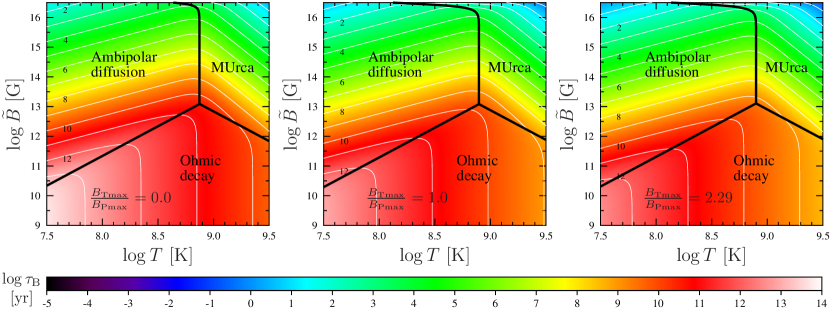
Figure 1: The magnetic field decay timescale $\tau_{\rm B}=2E_{\rm B}/\dot{E}_{\rm B}$ in the case of the non-equilibrium MUrca processes as the main mechanism restoring chemical equilibrium. From left to right: $B_{\rm Tmax}/B_{\rm Pmax}=0,\,1,\,2.29$. Thin white lines correspond to $\log\tau_{\rm B}={\rm const}$. Thick black lines in the ($\log\widetilde{B}-\log T$) plane separate the regions where one of the three dissipation mechanisms (ambipolar diffusion, MUrca processes, or Ohmic decay) is most efficient.

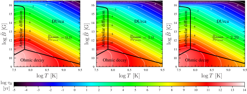
Figure 2: The same as in Fig. 1 but for the non-equilibrium DUrca process as the main mechanism that restores chemical equilibrium.

One can compare this dissipation rate with the total magnetic field energy stored in the core,

$$E_{\rm B}=\int_{V}\frac{\boldsymbol{B}^{2}}{8\pi}dV=\gamma\widetilde{B}_{14}^{2},$$ (87)

where the numerical factor $\gamma$ is also listed in Table 1. Figures 1 and 2 display the characteristic magnetic field decay timescale, $\tau_{\rm B}\equiv 2E_{\rm B}/\dot{E}_{\rm B}$, due to the mechanisms described above. Thick black lines separate regions where the contribution into $\tau_{\rm B}$ of one or another term in Eq. (86) is dominant. Thus, in the ‘MUrca’ and ‘DUrca’ domains the non-equilibrium beta-processes are the most important [first term in Eq. (86)]; in the “Ohmic decay” domain (second term) ohmic dissipation prevails; finally in the “ambipolar diffusion” domain the third term mostly determines the timescale $\tau_{\rm B}$. As we have already emphasized in Sec. V, this timescale coinci

des with the solenoidal ambipolar timescale from Ref. Goldreich and Reisenegger (1992).

As follows from the analysis of the figures, the boundary between the ambipolar diffusion and reaction (MUrca or DUrca) domains is independent of $\widetilde{B}$ at $\widetilde{B}\lesssim 10^{15}$ G. This means that the non-linear terms [see square bracket in Eq. (86)] are not important at such ${\widetilde{B}}$ and can be neglected. The non-linear regime of beta-reactions rapidly switches on at $\widetilde{B}\gtrsim 10^{16}$ G (MUrca) or $3\times 10^{15}$ G (DUrca). Note, however, that the magnetic fields that large become quantizing, which may affect the results quantitatively (but not qualitatively, see, e.g., Refs. Iakovlev and Shalybkov (1991); Baiko and Yakovlev (1999) and figure 3 in Ref. Yakovlev and Shalybkov (1991)). Second, there is a clear separation between the domains: the non-equilibrium beta-processes prevail at high $\widetilde{B}$ and $T$; ambipolar diffusion becomes important at relatively low temperature (the corresponding timescale scales as $1/T^{2}$), while the Ohmic decay plays a dominant role at low magnetic fields, but then the typical timescale exceeds the age of the Universe. Finally, one may note that when DUrca is switched on, it becomes the main dissipation mechanism in the almost whole region of $\widetilde{B}$ and $T$ shown in Fig. 2. Moreover, a typical timescale $\tau_{\rm B}$ for this mechanism can be very small, about a century for $T\gtrsim 6\times 10^{8}$ K and $\tilde{B}\sim 10^{14}$ G and 4–7 days for $\tilde{B}\sim 10^{16}$ G. The magnetic field will reconfigure (by effective dissipation) on these short timescales in order to vanish $\Delta\mu_{e}$ in the core, provided that the system evolves in the subthermal regime ($\Delta\mu_{e}\lesssim k_{\rm B}T$). The case of the suprathermal regime ($\Delta\mu_{e}\gtrsim k_{\rm B}T$) is a bit more tricky and will be analysed by us elsewhere.

VII Conclusions and final remarks

In this work we study the quasistationary equilibrium and dissipation in magnetized cores of NSs. We argue that the generally accepted approach to this problem pioneered by Goldreich and Reisenegger Goldreich and Reisenegger (1992) (see also Refs. Thompson and Duncan (1996); Hoyos et al. (2008); Reisenegger (2009); Hoyos et al. (2010); Glampedakis et al. (2011a); Beloborodov and Li (2016); Passamonti et al. (2017)) should be revised (see Appendix B for details). Taking, as an example, normal $npe$-matter in NS cores, we formulate a general scheme allowing one to find all the necessary ingredients (thermodynamic parameters, velocities, electric field, etc.) to self-consistently follow the quasistationary evolution of the stellar magnetic field. Our results can be summarized as follows:

• Expanding the quantities $\Delta\mu_{e}(r,\,\theta)\equiv\mu_{p}+\mu_{e}-\mu_{n}$ and $\delta\mu_{n}^{\infty}(r,\,\theta)$ in the Legendre polynomials $P_{l}({\rm cos}\theta)$, we demonstrate that all the components with $l\neq 0$ are fixed for stratified NSs by specifying the magnetic field configuration. This is in contrast to Refs. Thompson and Duncan (1996); Hoyos et al. (2008); Reisenegger (2009); Hoyos et al. (2010); Glampedakis et al. (2011a); Beloborodov and Li (2016); Passamonti et al. (2017), in which $\Delta\mu_{e}(r,\theta)$ is determined from a single scalar differential equation depending on both the beta-reaction coefficient $\lambda_{e}$ and the relaxation timescale $\tau_{np}$.

• The flow velocity ${\boldsymbol{U}}$, defined by Eq. (10), does not vanish and plays an important role in maintaining the quasi-equilibrium. Its components $U_{r}$ and $U_{\theta}$ can be found from the continuity equations (34) and (35), and they depend, in particular, on the sources $\Delta\Gamma$.

• The requirement of regularity of $U_{r}$ and $U_{\theta}$ at $r\rightarrow 0$, $\theta\rightarrow 0$, and $\theta\rightarrow\pi$ allows us to determine the $l=0$ components of the functions $\Delta\mu_{e}$ and $\delta\mu_{n}^{\infty}$ (Appendix D). It turns out that they depend on $T$ only in the narrow range of temperatures, where the dimensionless parameter $\lambda_{e}J_{np}R^{2}/n_{p}^{2}\sim 1$.

• The $\varphi$-component of the velocity ${\boldsymbol{U}}$ is of special interest. It should be chosen in such a way to ensure that the system is in the quasistationary state during its evolution [see the condition (40)].

• The results listed above are obtained for $npe$ composition of NS cores and for axisymmetric magnetic field configurations. However, they can be easily generalized to include muons (and other particle species), non-axisymmetric magnetic fields, and superfluidity/superconductivity (Secs. IV.1–IV.3). They can also be generalized to the case when there are other factors (in addition to the magnetic field) disturbing the system from the diffusion and beta-equilibrium (Sec. IV.4).

• We provide the formulas for the rate of magnetic field energy dissipation for both normal $npe$ and $npe\mu$-matter [see Eqs. (76) and (78)]. These formulas retain its form in the superfluid matter, see Ref. Kantor and Gusakov (2017). In the limiting case when electron-neutron collisions are neglected ($J_{en}=0$), our Eq. (76) reduces to the well-known result of Ref. Goldreich and Reisenegger (1992). What is more interesting, we formulate a theorem which states that, under quasistationary conditions (see Sec. III.1), all the heat generated in the system is due to dissipation of the magnetic energy, excluding possible losses through the system boundary, $\dot{E}_{\rm B}=-\int_{V}T\dot{S}\,dV+{\rm``Surface\,terms"}$.

• Our results are illustrated by a numerical example in which we calculate the dissipation timescales for the magnetic field as functions of typical field and temperature (Sec. VI). We demonstrate, in particular, that our ambipolar diffusion timescale coincides with the solenoidal ambipolar timescale of Ref. Goldreich and Reisenegger (1992), while the irrotational timescale (and the corresponding regime, see, e.g., Refs. Goldreich and Reisenegger (1992); Thompson and Duncan (1996); Arras et al. (2004); Hoyos et al. (2008); Reisenegger (2009); Dall’Osso et al. (2009); Hoyos et al. (2010); Glampedakis et al. (2011a); Dall’Osso et al. (2012); Beloborodov and Li (2016); Passamonti et al. (2017)) does not appear in our analysis.

• We see three immediate directions for future work. First, it would be extremely interesting to calculate the flow velocity ${\boldsymbol{U}}$ and hence to obtain all the necessary ingredients to follow the quasistationary magnetic field evolution in NSs. Second, an important problem concerns the topology of currents in the vicinity of the crust-core interface. How much magnetic energy flows away from the core and dissipates in the crust? This problem was completely ignored in the present paper. Third, the present work indicates the need to re-examine magnetothermal evolution of NSs, especially, magnetars. Could the observed surface temperature of magnetars be supported by the magnetic field dissipation in their cores? What is the role of suprathermal regime ($\Delta\mu_{e}\gtrsim k_{\rm B}T$) of beta-processes in such evolution? We hope to address these issues in our future work.

Appendix A Solution to Eq. (18)

Introducing the parameters $Z_{1}$ and $Z_{2}$,

$$Z_{1}=n_{e}\,\Delta\mu_{e}+n_{b}\,\delta\mu_{n}^{\infty},$$ (88)

$$Z_{2}=-\left(\frac{dn_{e}}{dr}\,\Delta\mu_{e}+\frac{dn_{b}}{dr}\,\delta\mu_{n}^{\infty}\right),$$ (89)

Eq. (18) can be rewritten as

$${\boldsymbol{\nabla}}Z_{1}+Z_{2}\,{\boldsymbol{e}}_{r}={\boldsymbol{F}}_{\rm L},$$ (90)

where ${\boldsymbol{F}}_{\rm L}=[{\boldsymbol{j}}\times{\boldsymbol{B}}]/c$ is the Lorentz force density. The solution to this equation reads

$$Z_{1}=\int_{0}^{\theta}rF_{{\rm L}\theta}\,d\tilde{\theta}+\zeta(r),$$ (91)

$$Z_{2}=F_{{\rm L}r}-\frac{\partial}{\partial r}\left[\int_{0}^{\theta}r\,F_{{\rm L}\theta}\,d\tilde{\theta}\right]-\zeta^{\prime}(r),$$ (92)

where the function $\zeta(r)$ is determined in Sec. III.3.1 (see also Appendix D). Using Eqs. (91) and (92), one finds

$$\left(\begin{array}[]{c}\Delta\mu_{e}\\ \delta\mu_{n}^{\infty}\end{array}\right)=\left(\begin{array}[]{cc}\,\,\,\,n_{e}&\,\,\,\,n_{b}\\ -\frac{dn_{e}}{dr}&-\frac{dn_{b}}{dr}\end{array}\right)^{-1}\left(\begin{array}[]{c}Z_{1}\\ Z_{2}\end{array}\right).$$ (99)

Note that, as follows from this equation, if we expand $\Delta\mu_{e}$ (or $\delta\mu_{n}^{\infty}$) in the series of Legendre polynomials $P_{l}({\rm cos\theta})$, $\Delta\mu_{e}=\sum_{l}\Delta\mu_{el}\,P_{l}({\rm cos}\theta)$, then the harmonics $\Delta\mu_{el}$ with $l\neq 0$ will be independent of $\zeta(r)$, i.e., they are fully determined by the magnetic field configuration.

Instead of the quantities $\Delta\mu_{e}$ and $\delta\mu_{n}^{\infty}$ it can be convenient to introduce the dimensionless parameters $\widetilde{\Delta\mu_{e}}$ and $\widetilde{\delta\mu_{n}^{\infty}}$ according to definitions

$$\Delta\mu_{e}\equiv\frac{\widetilde{B}^{2}}{\widetilde{n}}\,\widetilde{\Delta\mu_{e}},$$ (100)

$$\delta\mu_{n}^{\infty}\equiv\frac{\widetilde{B}^{2}}{\widetilde{n}}\,\widetilde{\delta\mu_{n}^{\infty}},$$ (101)

where $\widetilde{B}$ and $\widetilde{n}$ are some typical values of $B$ and number densities, respectively. The dimensionless parameter $\widetilde{\delta\mu_{n}^{\infty}}$ is of the order of $\widetilde{n}/(4\pi n_{b})$ in the star, while $\widetilde{\Delta\mu_{e}}\sim(n_{b}/n_{e})\,\widetilde{\delta\mu_{n}^{\infty}}$ for the magnetic field configurations considered in this paper.

Appendix B Traditional derivation of the scalar equation for $\Delta\mu_{e}$

Here we present the “traditional” derivation of the scalar equation for $\Delta\mu_{e}$ following the recent work Passamonti et al. (2017), and briefly discuss why (as we believe) the solution to this equation should not be relied upon. Below we consider $npe$-matter (i.e., $n_{e}=n_{p}$) and assume that $J_{en}=0$ (neutrons do not interact with electrons). Then, using Eqs. (16), (17), and (72), one obtains

$${\boldsymbol{\nabla}}\Delta\mu_{e}+\frac{\mu_{p}}{x_{n}^{2}c^{2}\tau_{pn}}\,{\boldsymbol{v}}_{\rm amb}=\frac{{\boldsymbol{F}_{\rm L}}}{n_{e}},$$ (102)

where ${\boldsymbol{v}}_{\rm amb}\equiv x_{n}({\boldsymbol{u}}_{p}-{\boldsymbol{u}}_{n})$; $x_{n}\equiv n_{n}/n_{b}$; $\tau_{pn}=\mu_{p}n_{p}/(c^{2}J_{np})$. Taking divergence of this equation and using the continuity equations (31)–(33), one finds

$${\rm div}{\boldsymbol{\nabla}}\Delta\mu_{e}-\frac{1}{b}\,\frac{\partial\Delta\mu_{e}}{\partial r}-\beta\,{\rm div}(n_{b}\,{\boldsymbol{u}}_{n})={\rm div}\left(\frac{{\boldsymbol{F}}_{\rm L}}{n_{e}}\right)-\frac{1}{b}\frac{F_{{\rm L}r}}{n_{e}},$$ (103)

where $1/b\equiv(1/\beta)\,d\beta/dr$ and $\beta\equiv\mu_{p}/(c^{2}x_{n}n_{p}\tau_{pn})$. The next step in the traditional approach consists in expressing ${\rm div}(n_{b}{\boldsymbol{u}}_{n})$ through $\Delta\mu_{e}$, which requires some further approximations Passamonti et al. (2017). For example, one can write (below we only consider the subthermal regime in which $\Delta\Gamma=\lambda_{e}\Delta\mu_{e}$; see Secs. V and VI for details)

$$x_{n}\,{\rm div}(n_{b}\,{\boldsymbol{u}}_{n})=x_{n}\,{\rm div}\left(\frac{{n_{n}}\,{\boldsymbol{u}}_{n}}{x_{n}}\right)=\lambda_{e}\Delta\mu_{e}-{\boldsymbol{\nabla}}x_{n}\,(n_{b}\,{\boldsymbol{u}}_{n})\approx\lambda_{e}\Delta\mu_{e},$$ (104)

where we, following Ref. Passamonti et al. (2017), neglected the term proportional to ${\boldsymbol{\nabla}}x_{n}$. Using this approximation, Eq. (103) takes the final form Passamonti et al. (2017)

$${\rm div}{\boldsymbol{\nabla}}\Delta\mu_{e}-\frac{1}{b}\,\frac{\partial\Delta\mu_{e}}{\partial r}-\frac{1}{a^{2}}\Delta\mu_{e}={\rm div}\left(\frac{{\boldsymbol{F}}_{\rm L}}{n_{e}}\right)-\frac{1}{b}\frac{F_{{\rm L}r}}{n_{e}},$$ (105)

where $1/a^{2}\equiv\beta\lambda_{e}/x_{n}$. The authors of Ref. Passamonti et al. (2017) impose the following boundary conditions for this equation: regularity of the ambipolar velocity at the origin and the magnetic axis, and vanishing of its radial component at the crust-core interface. With these boundary conditions Eq. (105) can be solved and it is easy to see that, generally, $\Delta\mu_{e}$ will depend on the relaxation time $\tau_{pn}$ and the beta-reaction rate (through the coefficient $\lambda_{e}$). This result apparently contradicts our solution (see Appendix A). Moreover, it follows from Eq. (105) that at large temperatures (when $1/a^{2}\rightarrow\infty$) $\Delta\mu_{e}=0$, while our solution (99) predicts that $\Delta\mu_{e}$ does not necessary vanish and is determined by the current magnetic field configuration (which, of course, will evolve in time to smooth out deviations from chemical equilibrium – but we do not consider the magnetic field dynamics in the present paper).

So, what is wrong with Eq. (105) and/or its solution? First of all, an approximation of Eq. (104), when one neglects the term $-{\boldsymbol{\nabla}}x_{n}\,(n_{b}\,{\boldsymbol{u}}_{n})$ in comparison to $\lambda_{e}\Delta\mu_{e}$ is unjustified, because ${\boldsymbol{u}}_{n}$ diverges at $\nabla x_{n}\rightarrow 0$ [see Eqs. (113) and (114) and the footnote 18]. Second, even if we take Eq. (105) for granted, it is not proven that the solution to this scalar equation is, at the same time, the solution to the initial vector equation (102) [or Eq. (16)]; our analysis shows that it is not the case.

Appendix C Magnetic field structure

We use the same axisymmetric model of the magnetic field as in Ref. Passamonti et al. (2017) (see this reference for a detailed description and justification of the model). In spherical coordinates the magnetic field is given by

$${\boldsymbol{B}}=\frac{1}{r\sin\theta}\left({\boldsymbol{\nabla}}\mathcal{P}\times{\boldsymbol{e}}_{\varphi}+\mathcal{T}{\boldsymbol{e}}_{\varphi}\right),$$ (106)

where ${\boldsymbol{e}}_{\varphi}$ is the unit vector in the azimuthal direction; $\mathcal{P}(r,\theta)$ and $\mathcal{T}(r,\theta)$ are the poloidal and toroidal stream functions, respectively. They are expressed as

$$\mathcal{P}=\mathcal{P}_{0}f(r/R_{\rm NS})\sin^{2}\theta,\qquad\mathcal{T}=\frac{s}{P_{0}R_{\rm NS}}\left(\mathcal{P}-\mathcal{P}_{0}\right)^{2}\Theta(\mathcal{P}-\mathcal{P}_{0}),$$ (107)

where $R_{\rm NS}$ is the stellar radius; $\Theta(x)$ is the Heaviside step function and the function

$$f(x)=\begin{cases}\frac{35}{8}x^{2}-\frac{21}{4}x^{4}+\frac{15}{8}x^{6},&x<1,\\ \frac{1}{x},&x\geqslant 1\end{cases}$$ (108)

determines one of the possible polynomial configurations of the poloidal component, which is dipolar outside the star. One can check that this magnetic field configuration satisfies the condition (19).

This model is defined by two parameters, $\mathcal{P}_{0}$ and $s$. It is more convenient, however, to choose the maximum absolute value of the poloidal $B_{\rm Pmax}$ and toroidal $B_{\rm Tmax}$ components as independent parameters. They are related to $\mathcal{P}_{0}$ and $s$ by the formulas

$$B_{\rm Pmax}=8.75\frac{\mathcal{P}_{0}}{R_{\rm NS}^{2}},\quad B_{\rm Tmax}\approx 0.0254\frac{s\mathcal{P}_{0}}{R_{\rm NS}^{2}},\quad s\approx 345\frac{B_{\rm Tmax}}{B_{\rm Pmax}}.$$ (109)

In addition, there is a magnetic field $B_{\rm p}$ at the pole on the stellar surface. From Eqs. (106)–(108) it follows that $B_{\rm p}\approx 0.229B_{\rm Pmax}$. Note that, at fixed ratio $B_{\rm Tmax}/B_{\rm Pmax}$, the magnetic field configuration is determined by the only one scaling parameter, e.g., $B_{\rm Pmax}$ or $B_{\rm p}$.

Appendix D Calculation of $\zeta(r)$

The general scheme of Sec. III.3.1 can be, of course, applied to the simple case of Sec. VI. However, it is easier to slightly modify it in this particular situation. Namely, it is convenient to start directly from the continuity equations (2) for protons and neutrons, which read, in the quasistationary approximation,

$$\frac{dn_{p}}{dr}u_{pr}+n_{p}\,{\rm div}\,{\boldsymbol{u}}_{p}=-\Delta\Gamma,$$ (110)

$$\frac{dn_{n}}{dr}u_{nr}+n_{n}\,{\rm div}\,{\boldsymbol{u}}_{n}=\Delta\Gamma,$$ (111)

where the number densities $n_{p}$, $n_{n}$ depend on $r$ only and $u_{pr}$, $u_{nr}$ are the radial components of the proton and neutron velocities ${\boldsymbol{u}}_{p}$ and ${\boldsymbol{u}}_{n}$, respectively. Note that these velocities are not independent. Assuming $J_{en}\ll J_{np}$, it follows from Eq. (72)

$${\boldsymbol{u}}_{p}={\boldsymbol{u}}_{n}+\frac{n_{n}}{J_{np}}\,{\boldsymbol{\nabla}}\delta\mu_{n}^{\infty}.$$ (112)

Using these equations, one can find ${\rm div}\,{\boldsymbol{u}}_{n}$ and $u_{nr}$:

$${\rm div}\,{\boldsymbol{u}}_{n}=-\frac{1}{y_{n}-y_{p}}\left[y_{n}\,{\rm div}\,{\boldsymbol{M}}_{n}+y_{n}y_{p}\,M_{nr}+\left(\frac{y_{p}}{n_{n}}+\frac{y_{n}}{n_{p}}\right)\,\Delta\Gamma\right],$$ (113)

$$u_{nr}=\frac{1}{y_{n}-y_{p}}\left[{\rm div}\,{\boldsymbol{M}}_{n}+y_{p}\,M_{nr}+\left(\frac{1}{n_{n}}+\frac{1}{n_{p}}\right)\Delta\Gamma\right],$$ (114)

where

$$y_{i}\equiv\frac{1}{n_{i}}\frac{dn_{i}}{dr},\quad i=n,\,p,$$ (115)

$${\boldsymbol{M}}_{n}\equiv\frac{n_{n}}{J_{np}}\,{\boldsymbol{\nabla}}\delta\mu_{n}^{\infty}.$$ (116)

Since $y_{i}\rightarrow O(r)$, at $r\rightarrow 0$, while $n_{n}$, $n_{p}$ and $J_{np}\rightarrow{\rm const}$ at $r\rightarrow 0$, it follows from Eq. (114) that $u_{nr}$ is finite at $r\rightarrow 0$ only if

$$\left[\frac{n_{n}}{J_{np}}\,\nabla^{2}(\delta\mu_{n}^{\infty})+\left(\frac{1}{n_{n}}+\frac{1}{n_{p}}\right)\Delta\Gamma\right]_{r\rightarrow 0}\sim r^{\alpha},\quad\alpha\geq 1.$$ (117)

Using Eqs. (113) and (114) we can find $u_{n\theta}$ and hence determine an analogue of the condition (37) ensuring finiteness of $u_{n\theta}$,

$$\int_{0}^{\pi}r\,{\rm sin}\tilde{\theta}\left[{\rm div}\,{\boldsymbol{u}}_{n}-\frac{1}{r^{2}}\frac{\partial(r^{2}u_{nr})}{\partial r}\right]d\tilde{\theta}=0.$$ (118)

This condition can be conveniently rewritten in an operator form as

$$\hat{\bf{P}}_{0}\left[{\rm div}\,{\boldsymbol{u}}_{n}-\frac{1}{r^{2}}\frac{\partial(r^{2}u_{nr})}{\partial r}\right]=0,$$ (119)

where the operator $\hat{\bf{P}}_{0}$ extracts $l=0$ component in the Legendre expansion of an arbitrary function $f(r,\,\theta)=\sum_{l=0}^{\infty}f_{l}(r)P_{l}({\rm cos}\,\theta)$: $\hat{\bf{P}}_{0}f(r,\,\theta)\equiv 1/2\,\int_{0}^{\pi}{\rm sin}\theta\,f(r,\,\theta)\,d\theta=f_{0}(r)$. Now, if we substitute Eqs. (113)–(116) into Eq. (119), we obtain a third-order linear differential equation depending on $(\hat{\bf{P}}_{0}\delta\mu_{n}^{\infty})^{\prime\prime\prime}$, $(\hat{\bf{P}}_{0}\delta\mu_{n}^{\infty})^{\prime\prime}$, $(\hat{\bf{P}}_{0}\delta\mu_{n}^{\infty})^{\prime}$, $(\hat{\bf{P}}_{0}\Delta\Gamma)^{\prime}$, and $\hat{\bf{P}}_{0}\Delta\Gamma$, where the prime (^′) means $d/dr$. Schematically, it can be presented as

$$A_{1}(r)\,(\hat{\bf{P}}_{0}\delta\mu_{n}^{\infty})^{\prime\prime\prime}+A_{2}(r)\,(\hat{\bf{P}}_{0}\delta\mu_{n}^{\infty})^{\prime\prime}+A_{3}(r)\,(\hat{\bf{P}}_{0}\delta\mu_{n}^{\infty})^{\prime}+A_{4}(r)\,(\hat{\bf{P}}_{0}\Delta\Gamma)^{\prime}+A_{5}(r)\,\hat{\bf{P}}_{0}\Delta\Gamma=0,$$ (120)

where $A_{1}(r)$, $A_{2}(r)$, $A_{3}(r)$, $A_{4}(r)$, and $A_{5}(r)$ are some coefficients that can be easily determined from Eqs. (113) and (114). Eq. (120) should be supplemented with the boundary conditions. They can be found, in particular, from Eq. (117), whose $l=0$ component is given by

$$\left[\frac{n_{n}}{J_{np}}\,\nabla^{2}(\hat{\bf{P}}_{0}\delta\mu_{n}^{\infty})+\left(\frac{1}{n_{n}}+\frac{1}{n_{p}}\right)\hat{\bf{P}}_{0}\Delta\Gamma\right]_{r\rightarrow 0}\sim r^{\alpha},\quad\alpha\geq 1.$$ (121)

Note that, Eqs. (120) and (121) depend on two functions, $\hat{\bf{P}}_{0}\delta\mu_{n}^{\infty}$ and $\hat{\bf{P}}_{0}\Delta\Gamma$. In fact, they are not independent and are related by the ($l=0$) radial component of Eq. (16), in which $\delta\Delta\mu_{e}^{\infty}=\Delta\mu_{e}$ [see Eq. (17)],

$$(\hat{\bf{P}}_{0}\delta\mu_{n}^{\infty})^{\prime}=\frac{1}{n_{b}}\,\hat{\bf{P}}_{0}F_{{\rm L}r}-\frac{n_{e}}{n_{b}}\,(\hat{\bf{P}}_{0}\Delta\mu_{e})^{\prime}.$$ (122)

Since $\Delta\Gamma$ is known function of $\Delta\mu_{e}$ [see Eqs. (84) and (85) in Sec. VI], and all the harmonics in the expansion of $\Delta\mu_{e}$ in Legendre polynomials except for $l=0$ are specified by the magnetic field [see Eq. (99)], the relation between $\hat{\bf{P}}_{0}\Delta\mu_{e}$ and $\hat{\bf{P}}_{0}\Delta\Gamma$ can be established after rather tedious but straightforward calculations. To simplify the subsequent presentation, below we consider the subthermal regime, $\Delta\mu_{e}\ll k_{\rm B}T$, in which $\Delta\Gamma=\lambda_{e}\Delta\mu_{e}$, where $\lambda_{e}$ is the beta-reaction coefficient that can be found from Eqs. (84) or (85).

Digression: Before proceeding further, let us make a following comment. It is easy to demonstrate that the last two terms in Eq. (120) [and the last term in Eq. (121)] can be neglected (i.e., beta-processes are not important) if $n_{p}^{2}/(R^{2}J_{np})\gg\lambda_{e}$ ($R$ is the typical lengthscale). Then Eq. (120) becomes a homogeneous differential equation with the boundary condition $\nabla^{2}(\hat{\bf{P}}_{0}\delta\mu_{n}^{\infty})|_{r\rightarrow 0}\sim r^{\alpha}$ ($\alpha\geq 1$) [see Eq. (121)], which results in $(\hat{\bf{P}}_{0}\delta\mu_{n}^{\infty})^{\prime}|_{r\rightarrow 0}=0$ and $(\hat{\bf{P}}_{0}\delta\mu_{n}^{\infty})^{\prime\prime}|_{r\rightarrow 0}=0$. It has a unique solution, $(\hat{\bf{P}}_{0}\delta\mu_{n}^{\infty})^{\prime}=0$, i.e., $\hat{\bf{P}}_{0}\delta\mu_{n}^{\infty}(r)=C$. The constant $C$ here is arbitrary; it specifies the central baryon number density of our perturbed NS model (following Ref. Hartle (1967), we prefer to define a stellar configuration by choosing central baryon density rather than the total number of baryons in the perturbed star). In what follows we assume $C=0$. In the opposite limit, $n_{p}^{2}/(R^{2}J_{np})\ll\lambda_{e}$ (diffusion is not efficient), similar consideration leads to the solution $\hat{\bf{P}}_{0}\Delta\Gamma(r)=0$, which reduces to $\hat{\bf{P}}_{0}\Delta\mu_{e}=0$ in the subthermal regime. Irrespective of the limit, knowledge of one function [$\hat{\bf{P}}_{0}\delta\mu_{n}^{\infty}$ or $\hat{\bf{P}}_{0}\Delta\mu_{e}$] allows one to determine the derivative of another function using Eq. (122).

As follows from these examples, the solution in both limits is not sensitive to the temperature or a particular dissipation mechanism. However, an interplay of the dissipation mechanisms (ambipolar diffusion and non-equilibrium beta-processes) determines a range of transition temperatures, defined by the condition $n_{p}^{2}/(R^{2}J_{np})\sim\lambda_{e}$, at which one asymptotic solution transforms into another. Since $\lambda_{e}$ is a strong function of temperature, the transition region is quite narrow.

Generally, to solve Eq. (120) with the boundary condition (121) one needs to express $(\hat{\bf{P}}_{0}\delta\mu_{n}^{\infty})^{\prime}$ in these equations through $\hat{\bf{P}}_{0}F_{{\rm L}r}$ and $(\hat{\bf{P}}_{0}\Delta\mu_{e})^{\prime}$ using Eq. (122). The resulting inhomogeneous differential equation allows one to determine the function $\hat{\bf{P}}_{0}\Delta\mu_{e}(r)$ (we remind that we assume $\hat{\bf{P}}_{0}\Delta\Gamma=\lambda_{e}\,\hat{\bf{P}}_{0}\Delta\mu_{e}$). The boundary conditions for $\hat{\bf{P}}_{0}\Delta\mu_{e}(r)$ depend on the behaviour of the magnetic field at $r\rightarrow 0$ and follow from the analysis of (121):

$$(\hat{\bf{P}}_{0}\Delta\mu_{e})^{\prime}|_{r\rightarrow 0}=0,$$ (123)

$$(\hat{\bf{P}}_{0}\Delta\mu_{e})^{\prime\prime}|_{r\rightarrow 0}=\left(\frac{1}{n_{e}}\,\hat{\bf{P}}_{0}F_{{\rm L}r}\right)^{\prime}|_{r\rightarrow 0}+\left(\frac{\lambda\,J_{np}\,n_{b}^{2}}{3\,n_{n}^{2}n_{p}^{2}}\,\hat{\bf{P}}_{0}\Delta\mu_{e}\right)|_{r\rightarrow 0}.$$ (124)

We have here only two boundary conditions, while to solve Eq. (120) we need, generally, one more condition which specifies $\hat{\bf{P}}_{0}\Delta\mu_{e}$ at some $r$. Presumably, this additional condition could be obtained by matching the solution of (120) with the solution of similar equation in the crust, but we have not tried to perform such an analysis. Let us only mention that in an idealised (and unrealistic) situation in which $\lambda=0$ in the crust (i.e., when beta-processes are suppressed in the crust) the condition for $\hat{\bf{P}}_{0}\Delta\mu_{e}$ could follow from the requirement that there are no net flow of neutrons from the core to the crust (otherwise, the quasistationarity condition would break down, since, by assumption, neutrons cannot be converted into protons in the crust). This requirement means $\int_{\rm core}\lambda\,(\hat{\bf{P}}_{0}\Delta\mu_{e})\,r^{2}dr=0$ [see Eq. (111)], which gives us a third necessary condition to solve (120).

Assuming that the functions $\hat{\bf{P}}_{0}\Delta\mu_{e}$ and $\hat{\bf{P}}_{0}\delta\mu_{n}^{\infty}$ are already defined, an unknown function $\zeta(r)$ can be found from the $l=0$ component of equation (91),

$$\zeta(r)=\hat{\bf{P}}_{0}Z_{1}-\hat{\bf{P}}_{0}\int_{0}^{\theta}r\,F_{{\rm L}\theta}\,d\tilde{\theta}.$$ (125)

The functions $\delta\mu_{n}^{\infty}(r,\,\theta)$ and $\Delta\mu_{e}(r,\,\theta)$ can then be found from Eq. (99). Alternatively, one can avoid use of the function $\zeta(r)$ by presenting the solution in the following equivalent way,

$$\delta\mu_{n}^{\infty}=(\delta\mu_{n}^{\infty})_{\rm A6}-\hat{\bf{P}}_{0}(\delta\mu_{n}^{\infty})_{\rm A6}+\hat{\bf{P}}_{0}\delta\mu_{n}^{\infty},$$ (126)

$$\Delta\mu_{e}=(\Delta\mu_{e})_{\rm A6}-\hat{\bf{P}}_{0}(\Delta\mu_{e})_{\rm A6}+\hat{\bf{P}}_{0}\Delta\mu_{e},$$ (127)

where the functions $(\delta\mu_{n}^{\infty})_{\rm A6}$ and $(\Delta\mu_{e})_{\rm A6}$ are given by Eq. (99). Although they depend on an (unknown) function $\zeta(r)$, one can choose this function in an arbitrary way (e.g., set $\zeta=0$) to calculate $(\delta\mu_{n}^{\infty})_{\rm A6}$ and $(\Delta\mu_{e})_{\rm A6}$, since it drops out from Eqs. (126) and (127).

To plot Figs. 1 and 2 we decided to use an approximate method for calculation of $\zeta(r)$. Namely, we employed the asymptotic solutions described above, assuming that $\hat{\bf{P}}_{0}\delta\mu_{n}^{\infty}(r)=0$ in the ambipolar diffusion domain (see Figs. 1 and 2) and $\hat{\bf{P}}_{0}\Delta\mu_{e}=0$ in the MUrca (DUrca) domain. We checked that the figures are not too sensitive to an actual form of the solution.

References

- Kaspi (2010) V. M. Kaspi, Proceedings of the National Academy of Science 107, 7147 (2010), eprint 1005.0876.
- Viganò et al. (2013) D. Viganò, N. Rea, J. A. Pons, R. Perna, D. N. Aguilera, and J. A. Miralles, Mon. Not. R. Astron. Soc. 434, 123 (2013), eprint 1306.2156.
- Haensel et al. (1990) P. Haensel, V. A. Urpin, and D. G. Iakovlev, Astron. Astrophys. 229, 133 (1990).
- Urpin and Shalybkov (1995) V. A. Urpin and D. A. Shalybkov, Astron. Astrophys. 294, 117 (1995).
- Page et al. (2000) D. Page, U. Geppert, and T. Zannias, Astron. Astrophys. 360, 1052 (2000), eprint astro-ph/0005301.
- Arras et al. (2004) P. Arras, A. Cumming, and C. Thompson, Astrophys. J. Lett. 608, L49 (2004), eprint astro-ph/0401561.
- Aguilera et al. (2008) D. N. Aguilera, J. A. Pons, and J. A. Miralles, Astron. Astrophys. 486, 255 (2008), eprint 0710.0854.
- Pons et al. (2009) J. A. Pons, J. A. Miralles, and U. Geppert, Astron. Astrophys. 496, 207 (2009), eprint 0812.3018.
- Jones (1988) P. B. Jones, Mon. Not. R. Astron. Soc. 233, 875 (1988).
- Shalybkov and Urpin (1997) D. A. Shalybkov and V. A. Urpin, Astron. Astrophys. 321, 685 (1997).
- Rheinhardt and Geppert (2002) M. Rheinhardt and U. Geppert, Physical Review Letters 88, 101103 (2002).
- Hollerbach and Rüdiger (2004) R. Hollerbach and G. Rüdiger, Mon. Not. R. Astron. Soc. 347, 1273 (2004).
- Gourgouliatos et al. (2013) K. N. Gourgouliatos, A. Cumming, A. Reisenegger, C. Armaza, M. Lyutikov, and J. A. Valdivia, Mon. Not. R. Astron. Soc. 434, 2480 (2013), eprint 1305.6269.
- Gourgouliatos and Cumming (2014) K. N. Gourgouliatos and A. Cumming, Physical Review Letters 112, 171101 (2014), eprint 1311.7345.
- Gourgouliatos et al. (2016) K. N. Gourgouliatos, T. S. Wood, and R. Hollerbach, Proceedings of the National Academy of Science 113, 3944 (2016), eprint 1604.01399.
- Baym et al. (1969) G. Baym, C. Pethick, and D. Pines, Nature (London) 224, 674 (1969).
- Pethick (1992) C. J. Pethick, in Structure and Evolution of Neutron Stars, edited by D. Pines, R. Tamagaki, and S. Tsuruta (1992), p. 115.
- Urpin and Ray (1994) V. A. Urpin and A. Ray, Mon. Not. R. Astron. Soc. 267, 1000 (1994).
- Thompson and Duncan (1996) C. Thompson and R. C. Duncan, Astrophys. J. 473, 322 (1996).
- Urpin and Shalybkov (1999) V. Urpin and D. Shalybkov, Mon. Not. R. Astron. Soc. 304, 451 (1999).
- Konenkov and Geppert (2000) D. Konenkov and U. Geppert, Mon. Not. R. Astron. Soc. 313, 66 (2000), eprint astro-ph/9910492.
- Konenkov and Geppert (2001) D. Konenkov and U. Geppert, Mon. Not. R. Astron. Soc. 325, 426 (2001), eprint astro-ph/0103060.
- Braithwaite and Spruit (2006) J. Braithwaite and H. C. Spruit, Astron. Astrophys. 450, 1097 (2006), eprint astro-ph/0510287.
- Hoyos et al. (2008) J. Hoyos, A. Reisenegger, and J. A. Valdivia, Astron. Astrophys. 487, 789 (2008), eprint 0801.4372.
- Dall’Osso et al. (2009) S. Dall’Osso, S. N. Shore, and L. Stella, Mon. Not. R. Astron. Soc. 398, 1869 (2009), eprint 0811.4311.
- Hoyos et al. (2010) J. H. Hoyos, A. Reisenegger, and J. A. Valdivia, Mon. Not. R. Astron. Soc. 408, 1730 (2010), eprint 1003.5262.
- Ho (2011) W. C. G. Ho, Mon. Not. R. Astron. Soc. 414, 2567 (2011), eprint 1102.4870.
- Dall’Osso et al. (2012) S. Dall’Osso, J. Granot, and T. Piran, Mon. Not. R. Astron. Soc. 422, 2878 (2012), eprint 1110.2498.
- Graber et al. (2015) V. Graber, N. Andersson, K. Glampedakis, and S. K. Lander, Mon. Not. R. Astron. Soc. 453, 671 (2015), eprint 1505.00124.
- Elfritz et al. (2016) J. G. Elfritz, J. A. Pons, N. Rea, K. Glampedakis, and D. Viganò, Mon. Not. R. Astron. Soc. 456, 4461 (2016), eprint 1512.07151.
- Beloborodov and Li (2016) A. M. Beloborodov and X. Li, Astrophys. J. 833, 261 (2016), eprint 1605.09077.
- Shalybkov and Urpin (1995) D. A. Shalybkov and V. A. Urpin, Mon. Not. R. Astron. Soc. 273, 643 (1995).
- Reisenegger (2009) A. Reisenegger, Astron. Astrophys. 499, 557 (2009), eprint 0809.0361.
- Glampedakis et al. (2011a) K. Glampedakis, D. I. Jones, and L. Samuelsson, Mon. Not. R. Astron. Soc. 413, 2021 (2011a), eprint 1010.1153.
- Passamonti et al. (2017) A. Passamonti, T. Akgün, J. A. Pons, and J. A. Miralles, Mon. Not. R. Astron. Soc. 465, 3416 (2017), eprint 1608.00001.
- Goldreich and Reisenegger (1992) P. Goldreich and A. Reisenegger, Astrophys. J. 395, 250 (1992).
- Iakovlev and Shalybkov (1991) D. G. Iakovlev and D. A. Shalybkov, Astrophys. Sp. Sci. 176, 171 (1991).
- Yakovlev et al. (2001) D. G. Yakovlev, A. D. Kaminker, O. Y. Gnedin, and P. Haensel, Phys. Rep. 354, 1 (2001), eprint astro-ph/0012122.
- Landau and Lifshitz (1960) L. D. Landau and E. M. Lifshitz, Electrodynamics of continuous media (1960).
- Braginskii (1965) S. I. Braginskii, in Reviews of Plasma Physics (Consultants Bureau, New York NY), edited by M. Leontovich (1965), vol. 1, p. 205.
- Reisenegger (2007) A. Reisenegger, Astronomische Nachrichten 328, 1173 (2007), eprint 0710.2839.
- Glampedakis and Lasky (2016) K. Glampedakis and P. D. Lasky, Mon. Not. R. Astron. Soc. 463, 2542 (2016), eprint 1607.05576.
- Kantor and Gusakov (2017) E. M. Kantor and M. E. Gusakov, Mon. Not. R. Astron. Soc. 473, 4272 (2018), eprint 1703.09216.
- Gusakov and Andersson (2006) M. E. Gusakov and N. Andersson, Mon. Not. R. Astron. Soc. 372, 1776 (2006), eprint astro-ph/0602282.
- Gusakov et al. (2009a) M. E. Gusakov, E. M. Kantor, and P. Haensel, Phys. Rev. C 79, 055806 (2009a), eprint 0904.3467.
- Gusakov et al. (2009b) M. E. Gusakov, E. M. Kantor, and P. Haensel, Phys. Rev. C 80, 015803 (2009b), eprint 0907.0010.
- Gusakov (2016) M. E. Gusakov, Phys. Rev. D 93, 064033 (2016), eprint 1601.07732.
- Gusakov and Dommes (2016) M. E. Gusakov and V. A. Dommes, Phys. Rev. D 94, 083006 (2016), eprint 1607.01629.
- Glampedakis et al. (2011b) K. Glampedakis, N. Andersson, and L. Samuelsson, Mon. Not. R. Astron. Soc. 410, 805 (2011b), eprint 1001.4046.
- Gusakov and Dommes (2017) M. E. Gusakov and V. A. Dommes, in preparation (2017).
- Yakovlev and Shalybkov (1990) D. G. Yakovlev and D. A. Shalybkov, Soviet Astronomy Letters 16, 86 (1990).
- Yakovlev and Shalybkov (1991) D. G. Yakovlev and D. A. Shalybkov, Astrophys. Space Sci. 176, 191 (1991).
- Reisenegger (1995) A. Reisenegger, Astrophys. J. 442, 749 (1995), eprint astro-ph/9410035.
- Shternin (2008) P. S. Shternin, Soviet Journal of Experimental and Theoretical Physics 107, 212 (2008).
- Heiselberg and Hjorth-Jensen (1999) H. Heiselberg and M. Hjorth-Jensen, Astrophys. J. Lett. 525, L45 (1999), eprint astro-ph/9904214.
- Jones (2001) P. B. Jones, Phys. Rev. D 64, 084003 (2001).
- Lindblom and Owen (2002) L. Lindblom and B. J. Owen, Phys. Rev. D 65, 063006 (2002), eprint astro-ph/0110558.
- Haensel et al. (2002) P. Haensel, K. P. Levenfish, and D. G. Yakovlev, Astron. Astrophys. 381, 1080 (2002), eprint astro-ph/0110575.
- Baiko and Yakovlev (1999) D. A. Baiko and D. G. Yakovlev, Astron. Astrophys. 342, 192 (1999), eprint astro-ph/9812071.
- Hartle (1967) J. B. Hartle, Astrophys. J. 150, 1005 (1967).