Non-linear perturbation of black branes at large D𝐷D

Umpei Miyamoto
RECCS, Akita Prefectural University, Akita 015-0055, Japan
umpei@akita-pu.ac.jp

1 Introduction

It is important to understand the dynamics of higher-dimensional black objects, since it tells us much about the nature of higher-dimensional gravitational theories and their holographically dual quantum field theories. The strong non-linearity of gravity, however, usually prevents us from understanding the dynamical properties of black objects beyond the linear-perturbation regime without highly sophisticated skills of numerical computation.

The Gregory-Laflamme (GL) instability [1], which is a universal instability of higher-dimensional black objects, is a good example to see the above situation. Though the GL instability in the non-linear regime is quite interesting, its analysis needs sophisticated skills of numerical relativity [2]. While there exists a semi-analytic higher-order perturbation method [3], it seems applicable only to static problems.

Recently, Emparan, Suzuki, and Tanabe showed that the Einstein equations describing the horizon dynamics of black branes in both Minkowski and Anti-de Sitter (AdS) background are recast in the form of coupled non-linear diffusion-type equations when the number of spatial dimensions is large [4]. This result provides us with a unique approach to the non-linear dynamics of black objects in higher dimensions. The authors indeed showed that the unstable black strings converge to non-uniform black strings (NUBSs), which had been predicted to happen above a critical dimension [5], by solving the diffusion equations numerically with a few lines of Mathematica code. It is added that the blackfold approach [6] is also thought to serve as a powerful approach to analyze the evolution of GL instability.

Once the simple diffusion equations were obtained [4], it is natural to ask if the non-linear properties of black-brane dynamics can be understood analytically. In this paper, we develop a systematic non-linear perturbation theory of asymptotically flat and AdS black branes, allowing the perturbations to be dynamical. Using the Fourier and Laplace transformation to solve the partial differential equations (PDEs), the perturbation equations are solved order by order for given arbitrary initial conditions up to the integration associated with the inverse transformation.

While the formulation is so general that it would be applicable to various problems, we pick up several examples as the initial conditions, which are a Gaussian wave packet, a step-function like shock configuration, and quite general discretely superposed sinusoidal waves. For these examples, the integration associated with the inverse transformation is completed up to the first or second order, and the properties of solutions are examined. Through these examples, one will see the validity of formalism itself and some unknown, or yet-to-be-confirmed, non-linear properties of black-brane dynamics. In particular, in the case of asymptotically flat black branes, an interesting non-liner property of GL instability resulting from the mode-mode coupling is unveiled at the second order. In the case of shock propagation on asymptotically AdS black branes, the analytic description of non-equilibrium steady state (NESS), which was recently discussed in the Riemann problem of relativistic fluid mechanics and field theories [7], is presented.

This paper is organized as follows. In Sec. 2, the asymptotically flat black branes are investigated. In Sec. 2.1, we present the perturbation equations for asymptotically flat black branes and their general form of solutions. In Sec. 2.2, we apply the general result to the Gaussian wave packet. In Sec. 2.3, we consider the discretely superposed sinusoidal waves. In Sec. 3, we consider the non-linear perturbation of asymptotically AdS black branes. Here, the formulation and applications are presented in parallel with Sec. 2, but a new example of initial condition, the step-function like shock, is investigated in Sec. 3.3. Section 4 is devoted to conclusion. Throughout this paper, we follow the notations in Ref. [4].

2 Asymptotically flat black branes

2.1 Perturbation equations and general form of solutions

In the large-D𝐷D(imension) approach, the horizon dynamics of vacuum black branes without a cosmological constant are described by two functions, m(t,z)𝑚𝑡𝑧m(t,z) and p(t,z)𝑝𝑡𝑧p(t,z), where t𝑡t is time and z𝑧z is the spatial coordinate along which the horizon extends [4]. m𝑚m and p𝑝p represent the mass and momentum distributions along the horizon, respectively. m+0𝑚0m\to+0 corresponds to the pinching off of the horizon. The equations of motion for these quantities take form of coupled non-linear diffusion equations,

(tz2)m+zp=0,subscript𝑡superscriptsubscript𝑧2𝑚subscript𝑧𝑝0\displaystyle(\partial_{t}-\partial_{z}^{2})m+\partial_{z}p=0, (2.1)
(tz2)pzm=z(p2m),subscript𝑡superscriptsubscript𝑧2𝑝subscript𝑧𝑚subscript𝑧superscript𝑝2𝑚\displaystyle(\partial_{t}-\partial_{z}^{2})p-\partial_{z}m=-\partial_{z}(\frac{p^{2}}{m}), (2.2)
t>0,<z<.formulae-sequence𝑡0𝑧\displaystyle t>0,\;\;\;-\infty<z<\infty. (2.3)

A uniform black-brane solution corresponds to m(t,z)1𝑚𝑡𝑧1m(t,z)\equiv 1 and p(t,z)0𝑝𝑡𝑧0p(t,z)\equiv 0. Since we are interested in the dynamical deformation of such a uniform solution, we introduce one-parameter families of m(t,z)𝑚𝑡𝑧m(t,z) and p(t,z)𝑝𝑡𝑧p(t,z), and expand them around the uniform black-brane solution,

m(t,z;ϵ)=1+=1m(t,z)ϵ,𝑚𝑡𝑧italic-ϵ1superscriptsubscript1subscript𝑚𝑡𝑧superscriptitalic-ϵ\displaystyle m(t,z;\epsilon)=1+\sum_{\ell=1}^{\infty}m_{\ell}(t,z)\epsilon^{\ell}, (2.4)
p(t,z;ϵ)==1p(t,z)ϵ,𝑝𝑡𝑧italic-ϵsuperscriptsubscript1subscript𝑝𝑡𝑧superscriptitalic-ϵ\displaystyle p(t,z;\epsilon)=\sum_{\ell=1}^{\infty}p_{\ell}(t,z)\epsilon^{\ell}, (2.5)

where ϵitalic-ϵ\epsilon is a constant parameterizing the families. Substituting these expansions into Eqs. (2.1) and (2.2), we obtain the equations of motion at O(ϵ)()𝑂superscriptitalic-ϵO(\epsilon^{\ell})\;(\ell\in{\mathbb{N}}),

m˙m′′+p=0,subscript˙𝑚superscriptsubscript𝑚′′superscriptsubscript𝑝0\displaystyle\dot{m}_{\ell}-m_{\ell}^{\prime\prime}+p_{\ell}^{\prime}=0, (2.6)
p˙p′′m=ψ,subscript˙𝑝superscriptsubscript𝑝′′superscriptsubscript𝑚subscript𝜓\displaystyle\dot{p}_{\ell}-p_{\ell}^{\prime\prime}-m_{\ell}^{\prime}=\psi_{\ell}, (2.7)

where the dot and prime denote the derivatives with respect to t𝑡t and z𝑧z, respectively. The right-hand side of Eq. (2.7), ψ(t,z)subscript𝜓𝑡𝑧\psi_{\ell}(t,z), which we call a source term, is a polynomial of the lower-order perturbations and their first spatial derivatives,

ψ10,subscript𝜓10\displaystyle\psi_{1}\equiv 0, (2.8)
ψ=ψ(m1,p1,m1,p1,,m1,p1,m1,p1),2.formulae-sequencesubscript𝜓subscript𝜓subscript𝑚1subscript𝑝1superscriptsubscript𝑚1superscriptsubscript𝑝1subscript𝑚1subscript𝑝1superscriptsubscript𝑚1superscriptsubscript𝑝12\displaystyle\psi_{\ell}=\psi_{\ell}(m_{1},p_{1},m_{1}^{\prime},p_{1}^{\prime},\cdots,m_{\ell-1},p_{\ell-1},m_{\ell-1}^{\prime},p_{\ell-1}^{\prime}),\;\;\;\ell\geq 2. (2.9)

For example, the source terms for =22\ell=2 and =33\ell=3 are given by

ψ2=2p1p1,subscript𝜓22subscript𝑝1superscriptsubscript𝑝1\displaystyle\psi_{2}=-2p_{1}p_{1}^{\prime}, (2.10)
ψ3=2m1p1p1+m1p122p1p22p1p2.subscript𝜓32subscript𝑚1subscript𝑝1superscriptsubscript𝑝1superscriptsubscript𝑚1superscriptsubscript𝑝122subscript𝑝1superscriptsubscript𝑝22superscriptsubscript𝑝1subscript𝑝2\displaystyle\psi_{3}=2m_{1}p_{1}p_{1}^{\prime}+m_{1}^{\prime}p_{1}^{2}-2p_{1}p_{2}^{\prime}-2p_{1}^{\prime}p_{2}. (2.11)

In the rest of this section, we are looking for the general form of solutions to the perturbation equations (2.6) and (2.7), combining the Fourier and Laplace transformations (see, e.g., [8]). A similar technique is found to be used in Ref. [9, 10] to analyze the higher-order perturbation of surface-diffusion equation, which is a single non-linear PDE.

Before starting to solve Eqs. (2.6) and (2.7), let us introduce the notations associated with the Fourier and Laplace transformations. For a given function, say f(t,z)𝑓𝑡𝑧f(t,z), we shall denote its Fourier transformation with respect to z𝑧z by f¯(t,k)¯𝑓𝑡𝑘\bar{f}(t,k), and its Laplace transformation with respect to t𝑡t by the corresponding capital letter F(s,z)𝐹𝑠𝑧F(s,z). Namely,

f¯(t,k)¯𝑓𝑡𝑘\displaystyle\bar{f}(t,k) :=[f(t,z)]=f(t,z)eikz𝑑z,i:=1,formulae-sequenceassignabsentdelimited-[]𝑓𝑡𝑧superscriptsubscript𝑓𝑡𝑧superscript𝑒𝑖𝑘𝑧differential-d𝑧assign𝑖1\displaystyle:={\cal F}[f(t,z)]=\int_{-\infty}^{\infty}f(t,z)e^{-ikz}dz,\;\;\;i:=\sqrt{-1}, (2.12)
F(s,z)𝐹𝑠𝑧\displaystyle F(s,z) :=[f(t,z)]=0f(t,z)est𝑑t.assignabsentdelimited-[]𝑓𝑡𝑧superscriptsubscript0𝑓𝑡𝑧superscript𝑒𝑠𝑡differential-d𝑡\displaystyle:={\cal L}[f(t,z)]=\int_{0}^{\infty}f(t,z)e^{-st}dt. (2.13)

Then, a capital letter with a bar denotes a Fourier-Laplace transformation as

F¯(s,k):=()[f(t,z)].assign¯𝐹𝑠𝑘delimited-[]𝑓𝑡𝑧\displaystyle\bar{F}(s,k):=({\cal L}\circ{\cal F})[f(t,z)]. (2.14)

In addition, we define two kind of convolutions,

f(t,z)g(t,z):=0tf(tτ,z)g(τ,z)𝑑τ,assign𝑓𝑡𝑧𝑔𝑡𝑧superscriptsubscript0𝑡𝑓𝑡𝜏𝑧𝑔𝜏𝑧differential-d𝜏\displaystyle f(t,z)\ast g(t,z):=\int_{0}^{t}f(t-\tau,z)g(\tau,z)d\tau, (2.15)
f(t,z)g(t,z):=f(t,zξ)g(τ,ξ)𝑑ξ.assign𝑓𝑡𝑧𝑔𝑡𝑧superscriptsubscript𝑓𝑡𝑧𝜉𝑔𝜏𝜉differential-d𝜉\displaystyle f(t,z)\star g(t,z):=\int_{-\infty}^{\infty}f(t,z-\xi)g(\tau,\xi)d\xi. (2.16)

With the notations introduced above, the Fourier-Laplace transformed version of Eqs. (2.6) and (2.7) are written as coupled algebraic equations in a matrix form

𝑨(M¯(s,k)P¯(s,k))=(m¯(0,k)p¯(0,k)+Ψ¯(s,k)),𝑨subscript¯𝑀𝑠𝑘subscript¯𝑃𝑠𝑘subscript¯𝑚0𝑘subscript¯𝑝0𝑘subscript¯Ψ𝑠𝑘\displaystyle{\bm{A}}\left(\begin{array}[]{c}\bar{M}_{\ell}(s,k)\\ \bar{P}_{\ell}(s,k)\\ \end{array}\right)=\left(\begin{array}[]{c}\bar{m}_{\ell}(0,k)\\ \bar{p}_{\ell}(0,k)+\bar{\Psi}_{\ell}(s,k)\\ \end{array}\right), (2.21)
𝑨:=(s+k2ikiks+k2),assign𝑨𝑠superscript𝑘2𝑖𝑘𝑖𝑘𝑠superscript𝑘2\displaystyle{\bm{A}}:=\left(\begin{array}[]{cc}s+k^{2}&ik\\ -ik&s+k^{2}\\ \end{array}\right), (2.24)

where we have used [znf(t,z)]=(ik)nf¯(t,k)(n)delimited-[]superscriptsubscript𝑧𝑛𝑓𝑡𝑧superscript𝑖𝑘𝑛¯𝑓𝑡𝑘𝑛{\cal F}[\partial_{z}^{n}f(t,z)]=(ik)^{n}\bar{f}(t,k)\;(n\in{\mathbb{N}}) and [tf(t,z)]=sF(s,z)f(0,z)delimited-[]subscript𝑡𝑓𝑡𝑧𝑠𝐹𝑠𝑧𝑓0𝑧{\cal L}[\partial_{t}f(t,z)]=sF(s,z)-f(0,z).

The solution to Eqs. (2.6) and (2.7) are obtained after multiplying Eq. (2.21) by 𝑨1superscript𝑨1{\bm{A}}^{-1} from left and inversely transforming it,

(m(t,z)p(t,z))=(11)[𝑨1(m¯(0,k)p¯(0,k)+Ψ¯(s,k))].subscript𝑚𝑡𝑧subscript𝑝𝑡𝑧superscript1superscript1delimited-[]superscript𝑨1subscript¯𝑚0𝑘subscript¯𝑝0𝑘subscript¯Ψ𝑠𝑘\displaystyle\left(\begin{array}[]{c}m_{\ell}(t,z)\\ p_{\ell}(t,z)\\ \end{array}\right)=({\cal F}^{-1}\circ{\cal L}^{-1})\left[{\bm{A}}^{-1}\left(\begin{array}[]{c}\bar{m}_{\ell}(0,k)\\ \bar{p}_{\ell}(0,k)+\bar{\Psi}_{\ell}(s,k)\\ \end{array}\right)\right]. (2.29)

By simple algebra, the inverse matrix 𝑨1superscript𝑨1{\bm{A}}^{-1} is found to be decomposed into two parts,

𝑨1=σ=+,1ssσ(k)𝑩σ,superscript𝑨1subscript𝜎1𝑠subscript𝑠𝜎𝑘subscript𝑩𝜎\displaystyle{\bm{A}}^{-1}=\sum_{\sigma=+,-}\frac{1}{s-s_{\sigma}(k)}{\bm{B}}_{\sigma}, (2.30)
𝑩σ:=12(1σiσi1),assignsubscript𝑩𝜎121𝜎𝑖𝜎𝑖1\displaystyle{\bm{B}}_{\sigma}:=\frac{1}{2}\left(\begin{array}[]{cc}1&-\sigma i\\ \sigma i&1\\ \end{array}\right), (2.33)
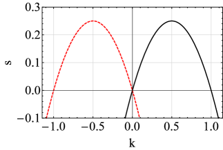
sσ(k):=k(σ1k).assignsubscript𝑠𝜎𝑘𝑘𝜎1𝑘\displaystyle s_{\sigma}(k):=k(\sigma 1-k). (2.34)

See Fig. 1 for plot of s=s±(k)𝑠subscript𝑠plus-or-minus𝑘s=s_{\pm}(k), which corresponds to the dispersion relation of waves.
Refer to caption
Figure 1: Dispersion relations s=s+(k)𝑠subscript𝑠𝑘s=s_{+}(k) (black solid) and s=s(k)𝑠subscript𝑠𝑘s=s_{-}(k) (red dashed), defined by Eq. (2.34).

After this decomposition, one can perform the inverse Laplace transformation 1superscript1{\cal L}^{-1} in Eq. (2.29) to obtain

(m(t,z)p(t,z))subscript𝑚𝑡𝑧subscript𝑝𝑡𝑧\displaystyle\left(\begin{array}[]{c}m_{\ell}(t,z)\\ p_{\ell}(t,z)\\ \end{array}\right) =σ=+,𝑩σ(1[esσ(k)tm¯(0,k)]1[esσ(k)tp¯(0,k)+esσ(k)tψ¯(t,k)])absentsubscript𝜎subscript𝑩𝜎superscript1delimited-[]superscript𝑒subscript𝑠𝜎𝑘𝑡subscript¯𝑚0𝑘superscript1delimited-[]superscript𝑒subscript𝑠𝜎𝑘𝑡subscript¯𝑝0𝑘superscript𝑒subscript𝑠𝜎𝑘𝑡subscript¯𝜓𝑡𝑘\displaystyle=\sum_{\sigma=+,-}{\bm{B}}_{\sigma}\left(\begin{array}[]{c}{\cal F}^{-1}[e^{s_{\sigma}(k)t}\bar{m}_{\ell}(0,k)]\\ {\cal F}^{-1}[e^{s_{\sigma}(k)t}\bar{p}_{\ell}(0,k)+e^{s_{\sigma}(k)t}\ast\bar{\psi}_{\ell}(t,k)]\\ \end{array}\right) (2.39)
=σ=+,𝑩σ(1[esσ(k)t]m(0,z)1[esσ(k)t]p(0,z)+1[esσ(k)t]ψ(t,z)).\displaystyle=\sum_{\sigma=+,-}{\bm{B}}_{\sigma}\left(\begin{array}[]{c}{\cal F}^{-1}[e^{s_{\sigma}(k)t}]\star m_{\ell}(0,z)\\ {\cal F}^{-1}[e^{s_{\sigma}(k)t}]\star p_{\ell}(0,z)+{\cal F}^{-1}[e^{s_{\sigma}(k)t}]\star\ast\psi_{\ell}(t,z)\\ \end{array}\right). (2.42)

Here, we have used 1[1sa]=eatsuperscript1delimited-[]1𝑠𝑎superscript𝑒𝑎𝑡{\cal L}^{-1}[\frac{1}{s-a}]=e^{at}, 1[F(s,z)G(s,z)]=f(t,z)g(t,z)superscript1delimited-[]𝐹𝑠𝑧𝐺𝑠𝑧𝑓𝑡𝑧𝑔𝑡𝑧{\cal L}^{-1}[F(s,z)G(s,z)]=f(t,z)\ast g(t,z), and 1[f¯(t,k)g¯(t,k)]=f(t,z)g(t,z)superscript1delimited-[]¯𝑓𝑡𝑘¯𝑔𝑡𝑘𝑓𝑡𝑧𝑔𝑡𝑧{\cal F}^{-1}[\bar{f}(t,k)\bar{g}(t,k)]=f(t,z)\star g(t,z).

Equations (2.39) and (2.42) are exactly what we wanted, namely, the general form of solutions to the perturbation equations (2.6) and (2.7) for given arbitrary initial conditions, m(0,z)subscript𝑚0𝑧m_{\ell}(0,z) and p(0,z)()subscript𝑝0𝑧p_{\ell}(0,z)\;(\ell\in{\mathbb{N}}). It depends on the problem which expression, (2.39) or (2.42), is easer to compute. For all examples considered in this paper, Eq. (2.39) seems easer to compute. Using Eq. (2.34), one can easily obtain

1[esσ(k)t]=14πtexp[(σt+iz)24t],superscript1delimited-[]superscript𝑒subscript𝑠𝜎𝑘𝑡14𝜋𝑡superscript𝜎𝑡𝑖𝑧24𝑡\displaystyle{\cal F}^{-1}[e^{s_{\sigma}(k)t}]=\frac{1}{\sqrt{4\pi t}}\exp[-\frac{(\sigma t+iz)^{2}}{4t}], (2.43)

which is useful when one uses expression (2.42).

In principle, one can obtain the arbitrary-order solutions, m(t,z)subscript𝑚𝑡𝑧m_{\ell}(t,z) and p(t,z)subscript𝑝𝑡𝑧p_{\ell}(t,z), by computing the right-hand side of Eq. (2.39) or (2.42) order by order. However, as the source term ψ(t,z)subscript𝜓𝑡𝑧\psi_{\ell}(t,z) becomes complicated as \ell increases, it is fare to say that to obtain the solutions analytically until arbitrary order is impossible in general. In addition, when the initial condition is a complicated function, even the first-order solution can be impossible to obtain analytically. Namely, the inverse Fourier transformation in Eq. (2.39) cannot be performed analytically in such a case. In the rest of this section, we shall consider two examples of initial conditions, for which the first few-order solutions are analytically obtainable.

2.2 Gaussian wave packet

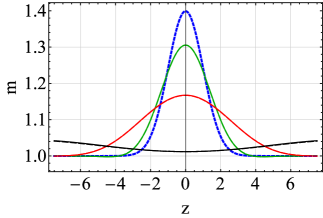
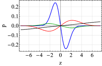
As the first example, we adopt the Gaussian wave packet as the initial perturbation given to the asymptotically flat black brane. For this perturbation, the inverse Fourier transformation at the first order in Eqs. (2.39) and (2.42) can be computed analytically. Since the unperturbed black brane is unstable, the perturbation of course grows unboundedly and nothing unexpected happens in this sense. However, one can see how to use the general results obtained in the previous section and the validity of the method. In particular, comparing the perturbative solution with a full numerical solution, the perturbative solution turns out to be effective even for finite-amplitude dynamics. In other words, the convergence of ϵitalic-ϵ\epsilon-expansion (2.4) and (2.5) is rapid enough at least for this example.

Let us assume that the situation where the black brane is given O(ϵ)𝑂italic-ϵO(\epsilon)-perturbation taking form of a Gaussian wave packet,

m1(0,z)=β2πbexp[(zz0)22b2],subscript𝑚10𝑧𝛽2𝜋𝑏superscript𝑧subscript𝑧022superscript𝑏2\displaystyle m_{1}(0,z)=\frac{\beta}{\sqrt{2\pi}b}\exp[-\frac{(z-z_{0})^{2}}{2b^{2}}], (2.44)
p1(0,z)=m1(0,z),subscript𝑝10𝑧superscriptsubscript𝑚10𝑧\displaystyle p_{1}(0,z)=m_{1}^{\prime}(0,z), (2.45)

where β,b(>0)𝛽annotated𝑏absent0\beta,\;b\;(>0), and z0subscript𝑧0z_{0} are real constants. Obviously, b𝑏b and z0subscript𝑧0z_{0} parameterize how much the wave packet spatially extends and the central position of the wave packet, respectively. β𝛽\beta is just a normalization constant to give m1(0,z)𝑑z=βsuperscriptsubscriptsubscript𝑚10𝑧differential-d𝑧𝛽\int_{-\infty}^{\infty}m_{1}(0,z)dz=\beta. The initial perturbation of p1subscript𝑝1p_{1} is given by the spatial derivative of m1subscript𝑚1m_{1} for simplicity, though their initial conditions can be independent in nature.

The Fourier transformation of the above initial conditions are

m¯1(0,k)=βexp[b2k22ikz0],subscript¯𝑚10𝑘𝛽superscript𝑏2superscript𝑘22𝑖𝑘subscript𝑧0\displaystyle\bar{m}_{1}(0,k)=\beta\exp[-\frac{b^{2}k^{2}}{2}-ikz_{0}], (2.46)
p¯1(0,k)=ikm¯1(0,k).subscript¯𝑝10𝑘𝑖𝑘subscript¯𝑚10𝑘\displaystyle\bar{p}_{1}(0,k)=ik\bar{m}_{1}(0,k). (2.47)

2.2.1 First-order solutions

Since we have no source term at O(ϵ)𝑂italic-ϵO(\epsilon), ψ1(t,z)0subscript𝜓1𝑡𝑧0\psi_{1}(t,z)\equiv 0, we see from Eq. (2.39) that what to compute is the inverse Fourier transformation of initial spectra, m¯1(0,k)subscript¯𝑚10𝑘\bar{m}_{1}(0,k) and p¯1(0,k)subscript¯𝑝10𝑘\bar{p}_{1}(0,k), multiplied by esσ(k)tsuperscript𝑒subscript𝑠𝜎𝑘𝑡e^{s_{\sigma}(k)t}. One can compute such quantities as

1[esσ(k)tm¯1(0,k)]superscript1delimited-[]superscript𝑒subscript𝑠𝜎𝑘𝑡subscript¯𝑚10𝑘\displaystyle{\cal F}^{-1}[e^{s_{\sigma}(k)t}\bar{m}_{1}(0,k)] =β2π(b2+2t)exp[t2(zz0)22(b2+2t)+iσt(zz0)b2+2t],absent𝛽2𝜋superscript𝑏22𝑡superscript𝑡2superscript𝑧subscript𝑧022superscript𝑏22𝑡𝑖𝜎𝑡𝑧subscript𝑧0superscript𝑏22𝑡\displaystyle=\frac{\beta}{\sqrt{2\pi(b^{2}+2t)}}\exp[\frac{t^{2}-(z-z_{0})^{2}}{2(b^{2}+2t)}+i\sigma\frac{t(z-z_{0})}{b^{2}+2t}], (2.48)
1[esσ(k)tp¯1(0,k)]superscript1delimited-[]superscript𝑒subscript𝑠𝜎𝑘𝑡subscript¯𝑝10𝑘\displaystyle{\cal F}^{-1}[e^{s_{\sigma}(k)t}\bar{p}_{1}(0,k)] =β[(zz0)iσt]2π(b2+2t)3exp[t2(zz0)22(b2+2t)+iσt(zz0)b2+2t].absent𝛽delimited-[]𝑧subscript𝑧0𝑖𝜎𝑡2𝜋superscriptsuperscript𝑏22𝑡3superscript𝑡2superscript𝑧subscript𝑧022superscript𝑏22𝑡𝑖𝜎𝑡𝑧subscript𝑧0superscript𝑏22𝑡\displaystyle=-\frac{\beta[(z-z_{0})-i\sigma t]}{\sqrt{2\pi(b^{2}+2t)^{3}}}\exp[\frac{t^{2}-(z-z_{0})^{2}}{2(b^{2}+2t)}+i\sigma\frac{t(z-z_{0})}{b^{2}+2t}]. (2.49)

Substituting these results into Eq. (2.39), we obtain the first-order solutions

(m1(t,z)p1(t,z))=β(b2+3t)2+(zz0)22π(b2+2t)3exp[t2(zz0)22(b2+2t)](cos[t(zz0)b2+2t+Θ]sin[t(zz0)b2+2t+Θ]),subscript𝑚1𝑡𝑧subscript𝑝1𝑡𝑧𝛽superscriptsuperscript𝑏23𝑡2superscript𝑧subscript𝑧022𝜋superscriptsuperscript𝑏22𝑡3superscript𝑡2superscript𝑧subscript𝑧022superscript𝑏22𝑡𝑡𝑧subscript𝑧0superscript𝑏22𝑡Θ𝑡𝑧subscript𝑧0superscript𝑏22𝑡Θ\displaystyle\left(\begin{array}[]{c}m_{1}(t,z)\\ p_{1}(t,z)\\ \end{array}\right)=\beta\sqrt{\frac{(b^{2}+3t)^{2}+(z-z_{0})^{2}}{2\pi(b^{2}+2t)^{3}}}\exp[\frac{t^{2}-(z-z_{0})^{2}}{2(b^{2}+2t)}]\left(\begin{array}[]{c}\displaystyle\cos[\frac{t(z-z_{0})}{b^{2}+2t}+\Theta]\\ \displaystyle-\sin[\frac{t(z-z_{0})}{b^{2}+2t}+\Theta]\\ \end{array}\right), (2.54)

where

cosΘ:=b2+3t(b2+3t)2+(zz0)2,sinΘ:=zz0(b2+3t)2+(zz0)2.formulae-sequenceassignΘsuperscript𝑏23𝑡superscriptsuperscript𝑏23𝑡2superscript𝑧subscript𝑧02assignΘ𝑧subscript𝑧0superscriptsuperscript𝑏23𝑡2superscript𝑧subscript𝑧02\displaystyle\cos\Theta:=\frac{b^{2}+3t}{\sqrt{(b^{2}+3t)^{2}+(z-z_{0})^{2}}},\;\;\;\sin\Theta:=\frac{z-z_{0}}{\sqrt{(b^{2}+3t)^{2}+(z-z_{0})^{2}}}. (2.55)

We believe that this is the first example describing the non-trivial evolution of GL instability analytically in time domain, which is realized by virtue of the large-D𝐷D method and perturbation theory developed in this paper.

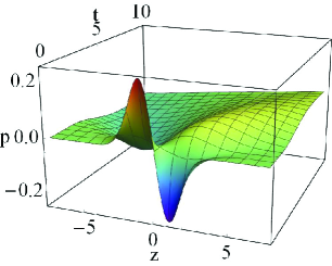
Like the diffusion phenomenon of a Gaussian wave packet according to an ordinary diffusion equation, solutions (2.54) have temporal decay factor, which behaves as 1b2+2t1superscript𝑏22𝑡\frac{1}{\sqrt{b^{2}+2t}}, and spatial decay factor exp[(zz0)22(b2+2t)]superscript𝑧subscript𝑧022superscript𝑏22𝑡\exp[-\frac{(z-z_{0})^{2}}{2(b^{2}+2t)}]. The sinusoidal parts represent spatial oscillation with time-dependent wavelength 2π(b2+2t)t2𝜋superscript𝑏22𝑡𝑡\frac{2\pi(b^{2}+2t)}{t}, which interestingly asymptotes to a universal value 4π4𝜋4\pi as t+𝑡t\to+\infty.

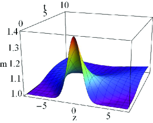
What crucially different from the ordinary diffusion is that the solutions temporally grow exponentially due to factor exp[t22(b2+2t)]superscript𝑡22superscript𝑏22𝑡\exp[\frac{t^{2}}{2(b^{2}+2t)}]. It is stressed that this exponential growing happens eventually irrespective of b𝑏b, which characterizes the extension of the initial wave packet. Substituting z=z0𝑧subscript𝑧0z=z_{0} into Eq. (2.54), we can see the time dependence of the peak height,

m1(t,z0)=β(b2+3t)22π(b2+2t)3exp[t22(b2+2t)].subscript𝑚1𝑡subscript𝑧0𝛽superscriptsuperscript𝑏23𝑡22𝜋superscriptsuperscript𝑏22𝑡3superscript𝑡22superscript𝑏22𝑡\displaystyle m_{1}(t,z_{0})=\beta\sqrt{\frac{(b^{2}+3t)^{2}}{2\pi(b^{2}+2t)^{3}}}\exp[\frac{t^{2}}{2(b^{2}+2t)}]. (2.56)

For b>3𝑏3b>\sqrt{3}, this is monotonically increasing in time. For 0<b<30𝑏30<b<\sqrt{3}, although it is initially decreasing, it turns increasing at t=13(32b2+b43b2+9)𝑡1332superscript𝑏2superscript𝑏43superscript𝑏29t=\frac{1}{3}(3-2b^{2}+\sqrt{b^{4}-3b^{2}+9}) to diverge eventually.

Thus, while the GL instability is generally said to be a long-wavelength instability, the initial perturbation taking form of a Gaussian wave packet necessarily grows exponentially however the ‘scale’ of perturbation b𝑏b is small. The reason is that the Fourier spectrum of any Gaussian wave packet necessarily contains the GL mode k(1,1){0}𝑘110k\in(-1,1)\setminus\{0\} (see Sec. 2.3.1). This is quite reasonable but might be a somewhat interesting point.

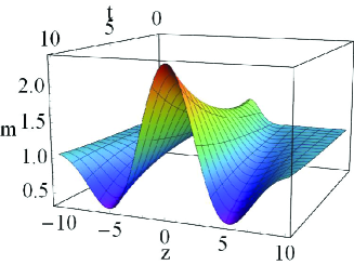
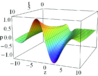
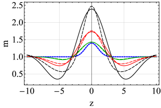
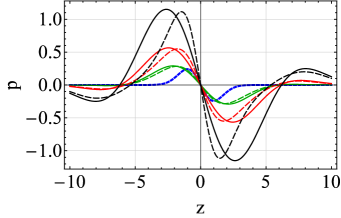
Three-dimensional plots of 1+m1(t,z)1subscript𝑚1𝑡𝑧1+m_{1}(t,z) and p1(t,z)subscript𝑝1𝑡𝑧p_{1}(t,z) are presented in Figs. 2(a) and 2(b), respectively. One can observe the growth and oscillation described above. In addition, snapshots of 1+m1(t,z)1subscript𝑚1𝑡𝑧1+m_{1}(t,z) and p1(t,z)subscript𝑝1𝑡𝑧p_{1}(t,z) at selected moments, compared with numerical solutions, are presented in Figs. 2(c) and 2(d), respectively. Compared with the full numerical solutions, which are obtained by directly solving original equations (2.1) and (2.2) with the same initial conditions, i.e., m(0,z)=1+m1(0,z)𝑚0𝑧1subscript𝑚10𝑧m(0,z)=1+m_{1}(0,z) and p(0,z)=p1(0,z)𝑝0𝑧subscript𝑝10𝑧p(0,z)=p_{1}(0,z), one can observe that the first-order solutions almost completely capture the qualitative features of the full solution during the time domain considered. Note that the deviation from the full solution, however, becomes large as the time proceeds, which results in the divergence of m𝑚m and p𝑝p.

2.2.2 Notes on second-order perturbation

The comparison between the first-order solution and full solution above tells us that O(ϵ2)𝑂superscriptitalic-ϵ2O(\epsilon^{2}) perturbations are negligible during the amplitudes of m𝑚m and p𝑝p are O(1)𝑂1O(1) in the current example despite the ordinary expectation that the perturbation becomes invalid for such a large amplitude. We will see in Sec. 3 that O(ϵ)𝑂italic-ϵO(\epsilon) approximation is more accurate for the Gaussian perturbation to the asymptotically AdS brane than the present case.

For the aim to see the non-linear effects at the second order, it is natural to assume that the initial perturbation at the second order vanishes, m2(0,z)=p2(0,z)=0subscript𝑚20𝑧subscript𝑝20𝑧0m_{2}(0,z)=p_{2}(0,z)=0. The reason is that m2(t,z)subscript𝑚2𝑡𝑧m_{2}(t,z) and p2(t,z)subscript𝑝2𝑡𝑧p_{2}(t,z) are composed of two independent parts as seen in Eq. (2.39): one is the contribution from initial perturbation m2(0,z)subscript𝑚20𝑧m_{2}(0,z) and p2(0,z)subscript𝑝20𝑧p_{2}(0,z), and the other is that from the source term ψ2(t,z)subscript𝜓2𝑡𝑧\psi_{2}(t,z). The former clearly has the same time dependence as the first term from Eq. (2.39). Namely, if we prepare the Gaussian wave packet as the initial condition of second-order perturbation, the second-order perturbation evolves in the exactly same way as the O(ϵ)𝑂italic-ϵO(\epsilon) perturbation described above. Only the latter, the contribution from the source term, can have a different time dependence from the first-order perturbation. This will be seen explicitly in Sec. 2.3.

From the reason described above, we should assume that the initial perturbations vanish at O(ϵ2)𝑂superscriptitalic-ϵ2O(\epsilon^{2}), m2(0,z)=p2(0,z)=0subscript𝑚20𝑧subscript𝑝20𝑧0m_{2}(0,z)=p_{2}(0,z)=0. Then, we see from Eq. (2.39) that what to compute at O(ϵ2)𝑂superscriptitalic-ϵ2O(\epsilon^{2}) is only the inverse Fourier transformation of the convolution between esσ(k)tsuperscript𝑒subscript𝑠𝜎𝑘𝑡e^{s_{\sigma}(k)t} and the spectrum of source term ψ¯2(t,k)subscript¯𝜓2𝑡𝑘\bar{\psi}_{2}(t,k). Unfortunately, however, such a convolution in the present example involves the Gauss error function, not written in terms of elementary functions. Thus, it seems difficult to obtain the second-order solutions analytically, and therefore we stop the analysis on this example here.

(a) (b)
Refer to caption Refer to caption
(c) (d)
Refer to caption Refer to caption
Figure 2: Three-dimensional plots of (a) 1+m1(t,z)1subscript𝑚1𝑡𝑧1+m_{1}(t,z) and (b) p1(t,z)subscript𝑝1𝑡𝑧p_{1}(t,z), given by Eqs. (2.54) with β=b=1,z0=0formulae-sequence𝛽𝑏1subscript𝑧00\beta=b=1,\;z_{0}=0. The comparison between first-order solution (c) 1+m1(t,z)1subscript𝑚1𝑡𝑧1+m_{1}(t,z) (resp. (d) p1(t,z)subscript𝑝1𝑡𝑧p_{1}(t,z)) and non-perturbative solution m(t,z)𝑚𝑡𝑧m(t,z) (resp. p(t,z)𝑝𝑡𝑧p(t,z)) obtained by numerically solving Eq. (2.1) and (2.2). The blue-dashed curve represents initial configuration m(0,z)𝑚0𝑧m(0,z) (resp. p(0,z)𝑝0𝑧p(0,z)). The green, red, and black solid curves represent the first-order solutions at t=3.3𝑡3.3t=3.3, 6.76.76.7, and 101010, respectively. The (green, red, and black) dashed curves represent the full numerical solutions at the corresponding time.

2.3 Superposed sinusoidal waves

As the second example, we consider the situation where the black brane is initially given an O(ϵ)𝑂italic-ϵO(\epsilon)-perturbation being a superposition of an arbitrary number of sinusoidal waves. This example is simple but interesting enough to see what happens in the non-linear regimes.

We set the following initial conditions

m1(0,z)=n=1Nancos(knz+φn),subscript𝑚10𝑧superscriptsubscript𝑛1𝑁subscript𝑎𝑛subscript𝑘𝑛𝑧subscript𝜑𝑛\displaystyle m_{1}(0,z)=\sum_{n=1}^{N}a_{n}\cos(k_{n}z+\varphi_{n}), (2.57)
p1(0,z)=m1(0,z),subscript𝑝10𝑧superscriptsubscript𝑚10𝑧\displaystyle p_{1}(0,z)=m_{1}^{\prime}(0,z), (2.58)
m(0,z)=p(0,z)=0,2,formulae-sequencesubscript𝑚0𝑧subscript𝑝0𝑧0for-all2\displaystyle m_{\ell}(0,z)=p_{\ell}(0,z)=0,\;\;\;\forall\ell\geq 2, (2.59)

where an,subscript𝑎𝑛a_{n}, knsubscript𝑘𝑛k_{n}, and φn(n=1,2,,N)subscript𝜑𝑛𝑛12𝑁\varphi_{n}\;(n=1,2,\cdots,N) are real constants. It is noted that the right-hand side of Eq. (2.57) is not written as the general form of Fourier series expansion of a periodic function. However, choosing appropriate wave number knsubscript𝑘𝑛k_{n} and phase φnsubscript𝜑𝑛\varphi_{n}, and taking summation over n𝑛n from 00 to infinity, rather than from 1 to N𝑁N, Eq. (2.57) can cover the Fourier series expansion of arbitrary piecewise continuous periodic function. The assumption that the second and higher order perturbations vanish initially are adopted from the same reason as the previous example in Sec. 2.2.

The Fourier transformations of the above initial configurations are

m¯1(0,k)=πn=1Nan[eiφnδ(kkn)+eiφnδ(k+kn)],subscript¯𝑚10𝑘𝜋superscriptsubscript𝑛1𝑁subscript𝑎𝑛delimited-[]superscript𝑒𝑖subscript𝜑𝑛𝛿𝑘subscript𝑘𝑛superscript𝑒𝑖subscript𝜑𝑛𝛿𝑘subscript𝑘𝑛\displaystyle\bar{m}_{1}(0,k)=\pi\sum_{n=1}^{N}a_{n}[e^{i\varphi_{n}}\delta(k-k_{n})+e^{-i\varphi_{n}}\delta(k+k_{n})], (2.60)
p¯1(0,k)=ikm¯1(0,k),subscript¯𝑝10𝑘𝑖𝑘subscript¯𝑚10𝑘\displaystyle\bar{p}_{1}(0,k)=ik\bar{m}_{1}(0,k), (2.61)
m¯(0,k)=p¯(0,k)=0,2.formulae-sequencesubscript¯𝑚0𝑘subscript¯𝑝0𝑘0for-all2\displaystyle\bar{m}_{\ell}(0,k)=\bar{p}_{\ell}(0,k)=0,\;\;\;\forall\ell\geq 2. (2.62)

In the rest of this section, we shall compute the right-hand side of Eq. (2.39) order by order for these initial conditions.

2.3.1 First-order solutions

Since we have no source term at O(ϵ)𝑂italic-ϵO(\epsilon), ψ10subscript𝜓10\psi_{1}\equiv 0, we see from Eq. (2.39) that what to compute is only the inverse Fourier transformation of the initial spectra, m¯1(0,k)subscript¯𝑚10𝑘\bar{m}_{1}(0,k) and q¯1(0,k)subscript¯𝑞10𝑘\bar{q}_{1}(0,k), multiplied by esσ(k)tsuperscript𝑒subscript𝑠𝜎𝑘𝑡e^{s_{\sigma}(k)t}. These are easily computed to give

1[esσ(k)tm¯1(0,k)]=superscript1delimited-[]superscript𝑒subscript𝑠𝜎𝑘𝑡subscript¯𝑚10𝑘absent\displaystyle{\cal F}^{-1}[e^{s_{\sigma}(k)t}\bar{m}_{1}(0,k)]= 12n=1Nan[esσ(kn)tei(knz+φn)+esσ(kn)tei(knz+φn)],12superscriptsubscript𝑛1𝑁subscript𝑎𝑛delimited-[]superscript𝑒subscript𝑠𝜎subscript𝑘𝑛𝑡superscript𝑒𝑖subscript𝑘𝑛𝑧subscript𝜑𝑛superscript𝑒subscript𝑠𝜎subscript𝑘𝑛𝑡superscript𝑒𝑖subscript𝑘𝑛𝑧subscript𝜑𝑛\displaystyle\frac{1}{2}\sum_{n=1}^{N}a_{n}[e^{s_{\sigma}(k_{n})t}e^{i(k_{n}z+\varphi_{n})}+e^{s_{-\sigma}(k_{n})t}e^{-i(k_{n}z+\varphi_{n})}], (2.63)
1[esσ(k)tp¯1(0,k)]=superscript1delimited-[]superscript𝑒subscript𝑠𝜎𝑘𝑡subscript¯𝑝10𝑘absent\displaystyle{\cal F}^{-1}[e^{s_{\sigma}(k)t}\bar{p}_{1}(0,k)]= i2n=1Nknan[esσ(kn)tei(knz+φn)esσ(kn)tei(knz+φn)],𝑖2superscriptsubscript𝑛1𝑁subscript𝑘𝑛subscript𝑎𝑛delimited-[]superscript𝑒subscript𝑠𝜎subscript𝑘𝑛𝑡superscript𝑒𝑖subscript𝑘𝑛𝑧subscript𝜑𝑛superscript𝑒subscript𝑠𝜎subscript𝑘𝑛𝑡superscript𝑒𝑖subscript𝑘𝑛𝑧subscript𝜑𝑛\displaystyle\frac{i}{2}\sum_{n=1}^{N}k_{n}a_{n}[e^{s_{\sigma}(k_{n})t}e^{i(k_{n}z+\varphi_{n})}-e^{s_{-\sigma}(k_{n})t}e^{-i(k_{n}z+\varphi_{n})}], (2.64)

where we have used sσ(k)=sσ(k)subscript𝑠𝜎𝑘subscript𝑠𝜎𝑘s_{\sigma}(-k)=s_{-\sigma}(k). Substituting these results into Eq. (2.39), we obtain the first-order solutions,

m1(t,z)=subscript𝑚1𝑡𝑧absent\displaystyle m_{1}(t,z)= 12n=1Nan[(1+kn)es+(kn)t+(1kn)es(kn)t]cos(knz+φn),12superscriptsubscript𝑛1𝑁subscript𝑎𝑛delimited-[]1subscript𝑘𝑛superscript𝑒subscript𝑠subscript𝑘𝑛𝑡1subscript𝑘𝑛superscript𝑒subscript𝑠subscript𝑘𝑛𝑡subscript𝑘𝑛𝑧subscript𝜑𝑛\displaystyle\frac{1}{2}\sum_{n=1}^{N}a_{n}[(1+k_{n})e^{s_{+}(k_{n})t}+(1-k_{n})e^{s_{-}(k_{n})t}]\cos(k_{n}z+\varphi_{n}), (2.65)
p1(t,z)=subscript𝑝1𝑡𝑧absent\displaystyle p_{1}(t,z)= 12n=1Nan[(1+kn)es+(kn)t(1kn)es(kn)t]sin(knz+φn).12superscriptsubscript𝑛1𝑁subscript𝑎𝑛delimited-[]1subscript𝑘𝑛superscript𝑒subscript𝑠subscript𝑘𝑛𝑡1subscript𝑘𝑛superscript𝑒subscript𝑠subscript𝑘𝑛𝑡subscript𝑘𝑛𝑧subscript𝜑𝑛\displaystyle-\frac{1}{2}\sum_{n=1}^{N}a_{n}[(1+k_{n})e^{s_{+}(k_{n})t}-(1-k_{n})e^{s_{-}(k_{n})t}]\sin(k_{n}z+\varphi_{n}). (2.66)

Equations (2.65) and (2.66) represent O(ϵ)𝑂italic-ϵO(\epsilon) approximate time evolution of the initial perturbation, which takes the form of superposed sinusoidal waves (2.57) and (2.58). Since the initial conditions (2.57) and (2.58) are quite general, so are the solutions (2.65) and (2.66).

Since we are considering linear equations of motion, there is no mode-mode coupling appearing in non-linear regime, and therefore Eqs. (2.65) and (2.66) have simple interpretation. The factor of cos(knz+φn)subscript𝑘𝑛𝑧subscript𝜑𝑛\cos(k_{n}z+\varphi_{n}) in Eq. (2.65) represents the time-dependent amplitude of the initially given mode cos(knz+φn)subscript𝑘𝑛𝑧subscript𝜑𝑛\cos(k_{n}z+\varphi_{n}). Each mode evolves independently according to its growth or damping rate determined by es+(kn)tsuperscript𝑒subscript𝑠subscript𝑘𝑛𝑡e^{s_{+}(k_{n})t} and es(kn)tsuperscript𝑒subscript𝑠subscript𝑘𝑛𝑡e^{s_{-}(k_{n})t}. From the concrete form of s±(k)subscript𝑠plus-or-minus𝑘s_{\pm}(k) in Eq. (2.34), one can see that if kn(1,0)subscript𝑘𝑛10k_{n}\in(-1,0) (resp. kn(0,1)subscript𝑘𝑛01k_{n}\in(0,1)), such a mode grows exponentially due to es(kn)tsuperscript𝑒subscript𝑠subscript𝑘𝑛𝑡e^{s_{-}(k_{n})t} (resp. es+(kn)tsuperscript𝑒subscript𝑠subscript𝑘𝑛𝑡e^{s_{+}(k_{n})t}), which represents the GL instability.

2.3.2 Second-order solutions

Since we assume that the initial perturbations vanish at O(ϵ2)𝑂superscriptitalic-ϵ2O(\epsilon^{2}), m2(0,z)=p2(0,z)=0subscript𝑚20𝑧subscript𝑝20𝑧0m_{2}(0,z)=p_{2}(0,z)=0, we see from Eq. (2.39) that what to compute is the inverse Fourier transformation of the convolution between esσ(k)tsuperscript𝑒subscript𝑠𝜎𝑘𝑡e^{s_{\sigma}(k)t} and the Fourier spectrum of source term ψ¯2(t,k)subscript¯𝜓2𝑡𝑘\bar{\psi}_{2}(t,k). Using Eqs. (2.10) and (2.66), such a quantity is computed and written down in a simple form as

1[esσ(k)t\displaystyle{\cal F}^{-1}[e^{s_{\sigma}(k)t}\ast ψ¯2(t,k)]=i8n=1Nn=1Nanankn\displaystyle\bar{\psi}_{2}(t,k)]=\frac{i}{8}\sum_{n=1}^{N}\sum_{n^{\prime}=1}^{N}a_{n}a_{n^{\prime}}k_{n^{\prime}}
×(Cnn(σ)(+)ei[(kn+kn)z+(φn+φn)]+Cnn(σ)()ei[(knkn)z+(φnφn)]\displaystyle\times\Big{(}C_{nn^{\prime}}^{(\sigma)(+)}e^{i[(k_{n}+k_{n^{\prime}})z+(\varphi_{n}+\varphi_{n^{\prime}})]}+C_{nn^{\prime}}^{(\sigma)(-)}e^{i[(k_{n}-k_{n^{\prime}})z+(\varphi_{n}-\varphi_{n^{\prime}})]}
Cnn(σ)()ei[(knkn)z+(φnφn)]Cnn(σ)(+)ei[(kn+kn)z+(φn+φn)])\displaystyle-C_{nn^{\prime}}^{(-\sigma)(-)}e^{-i[(k_{n}-k_{n^{\prime}})z+(\varphi_{n}-\varphi_{n^{\prime}})]}-C_{nn^{\prime}}^{(-\sigma)(+)}e^{-i[(k_{n}+k_{n^{\prime}})z+(\varphi_{n}+\varphi_{n^{\prime}})]}\Big{)} (2.67)

by defining a function of time,

Cnn(σ)(σ):=assignsuperscriptsubscript𝐶𝑛superscript𝑛𝜎superscript𝜎absent\displaystyle C_{nn^{\prime}}^{(\sigma)(\sigma^{\prime})}:= (1+kn)(1+kn)s+(kn)+s+(kn)sσ(kn+σkn)(e[s+(kn)+s+(kn)]tesσ(kn+σkn)t)1subscript𝑘𝑛1subscript𝑘superscript𝑛subscript𝑠subscript𝑘𝑛subscript𝑠subscript𝑘superscript𝑛subscript𝑠𝜎subscript𝑘𝑛superscript𝜎subscript𝑘superscript𝑛superscript𝑒delimited-[]subscript𝑠subscript𝑘𝑛subscript𝑠subscript𝑘superscript𝑛𝑡superscript𝑒subscript𝑠𝜎subscript𝑘𝑛superscript𝜎subscript𝑘superscript𝑛𝑡\displaystyle\frac{(1+k_{n})(1+k_{n^{\prime}})}{s_{+}(k_{n})+s_{+}(k_{n^{\prime}})-s_{\sigma}(k_{n}+\sigma^{\prime}k_{n^{\prime}})}(e^{[s_{+}(k_{n})+s_{+}(k_{n^{\prime}})]t}-e^{s_{\sigma}(k_{n}+\sigma^{\prime}k_{n^{\prime}})t})
\displaystyle- (1+kn)(1kn)s+(kn)+s(kn)sσ(kn+σkn)(e[s+(kn)+s(kn)]tesσ(kn+σkn)t)1subscript𝑘𝑛1subscript𝑘superscript𝑛subscript𝑠subscript𝑘𝑛subscript𝑠subscript𝑘superscript𝑛subscript𝑠𝜎subscript𝑘𝑛superscript𝜎subscript𝑘superscript𝑛superscript𝑒delimited-[]subscript𝑠subscript𝑘𝑛subscript𝑠subscript𝑘superscript𝑛𝑡superscript𝑒subscript𝑠𝜎subscript𝑘𝑛superscript𝜎subscript𝑘superscript𝑛𝑡\displaystyle\frac{(1+k_{n})(1-k_{n^{\prime}})}{s_{+}(k_{n})+s_{-}(k_{n^{\prime}})-s_{\sigma}(k_{n}+\sigma^{\prime}k_{n^{\prime}})}(e^{[s_{+}(k_{n})+s_{-}(k_{n^{\prime}})]t}-e^{s_{\sigma}(k_{n}+\sigma^{\prime}k_{n^{\prime}})t})
\displaystyle- (1kn)(1+kn)s(kn)+s+(kn)sσ(kn+σkn)(e[s(kn)+s+(kn)]tesσ(kn+σkn)t)1subscript𝑘𝑛1subscript𝑘superscript𝑛subscript𝑠subscript𝑘𝑛subscript𝑠subscript𝑘superscript𝑛subscript𝑠𝜎subscript𝑘𝑛superscript𝜎subscript𝑘superscript𝑛superscript𝑒delimited-[]subscript𝑠subscript𝑘𝑛subscript𝑠subscript𝑘superscript𝑛𝑡superscript𝑒subscript𝑠𝜎subscript𝑘𝑛superscript𝜎subscript𝑘superscript𝑛𝑡\displaystyle\frac{(1-k_{n})(1+k_{n^{\prime}})}{s_{-}(k_{n})+s_{+}(k_{n^{\prime}})-s_{\sigma}(k_{n}+\sigma^{\prime}k_{n^{\prime}})}(e^{[s_{-}(k_{n})+s_{+}(k_{n^{\prime}})]t}-e^{s_{\sigma}(k_{n}+\sigma^{\prime}k_{n^{\prime}})t})
+\displaystyle+ (1kn)(1kn)s(kn)+s(kn)sσ(kn+σkn)(e[s(kn)+s(kn)]tesσ(kn+σkn)t).1subscript𝑘𝑛1subscript𝑘superscript𝑛subscript𝑠subscript𝑘𝑛subscript𝑠subscript𝑘superscript𝑛subscript𝑠𝜎subscript𝑘𝑛superscript𝜎subscript𝑘superscript𝑛superscript𝑒delimited-[]subscript𝑠subscript𝑘𝑛subscript𝑠subscript𝑘superscript𝑛𝑡superscript𝑒subscript𝑠𝜎subscript𝑘𝑛superscript𝜎subscript𝑘superscript𝑛𝑡\displaystyle\frac{(1-k_{n})(1-k_{n^{\prime}})}{s_{-}(k_{n})+s_{-}(k_{n^{\prime}})-s_{\sigma}(k_{n}+\sigma^{\prime}k_{n^{\prime}})}(e^{[s_{-}(k_{n})+s_{-}(k_{n^{\prime}})]t}-e^{s_{\sigma}(k_{n}+\sigma^{\prime}k_{n^{\prime}})t}). (2.68)

Substituting the above result (2.67) into Eq. (2.39), we obtain the second-order solutions,

m2(t,z)=18n=1nn=1Nanankn([\displaystyle m_{2}(t,z)=\frac{1}{8}\sum_{n=1}^{n}\sum_{n^{\prime}=1}^{N}a_{n}a_{n^{\prime}}k_{n^{\prime}}\Big{(}[ Cnn(+)(+)Cnn()(+)]cos[(kn+kn)z+(φn+φn)]\displaystyle C_{nn^{\prime}}^{(+)(+)}-C_{nn^{\prime}}^{(-)(+)}]\cos[(k_{n}+k_{n^{\prime}})z+(\varphi_{n}+\varphi_{n^{\prime}})]
+\displaystyle+ [Cnn(+)()Cnn()()]cos[(knkn)z+(φnφn)]),\displaystyle[C_{nn^{\prime}}^{(+)(-)}-C_{nn^{\prime}}^{(-)(-)}]\cos[(k_{n}-k_{n^{\prime}})z+(\varphi_{n}-\varphi_{n^{\prime}})]\Big{)}, (2.69)
p2(t,z)=18n=1nn=1Nanankn([\displaystyle p_{2}(t,z)=-\frac{1}{8}\sum_{n=1}^{n}\sum_{n^{\prime}=1}^{N}a_{n}a_{n^{\prime}}k_{n^{\prime}}\Big{(}[ Cnn(+)(+)+Cnn()(+)]sin[(kn+kn)z+(φn+φn)]\displaystyle C_{nn^{\prime}}^{(+)(+)}+C_{nn^{\prime}}^{(-)(+)}]\sin[(k_{n}+k_{n^{\prime}})z+(\varphi_{n}+\varphi_{n^{\prime}})]
+\displaystyle+ [Cnn(+)()+Cnn()()]sin[(knkn)z+(φnφn)]).\displaystyle[C_{nn^{\prime}}^{(+)(-)}+C_{nn^{\prime}}^{(-)(-)}]\sin[(k_{n}-k_{n^{\prime}})z+(\varphi_{n}-\varphi_{n^{\prime}})]\Big{)}. (2.70)

Note that m(t,z)=1+m1(t,z)+m2(t,z)𝑚𝑡𝑧1subscript𝑚1𝑡𝑧subscript𝑚2𝑡𝑧m(t,z)=1+m_{1}(t,z)+m_{2}(t,z) and p(t,z)=p1(t,z)+p2(t,z)𝑝𝑡𝑧subscript𝑝1𝑡𝑧subscript𝑝2𝑡𝑧p(t,z)=p_{1}(t,z)+p_{2}(t,z) with Eqs. (2.65), (2.66), (2.69), and (2.70), represent O(ϵ2)𝑂superscriptitalic-ϵ2O(\epsilon^{2}) approximate time evolution of the initial perturbation, which takes the form of superposed sinusoidal waves (2.57), (2.58), and (2.59). Since the initial conditions (2.57) and (2.58) are quite general, so are these approximate solutions.

Since the initial perturbations are assumed to vanish at O(ϵ2)𝑂superscriptitalic-ϵ2O(\epsilon^{2}), m2(0,z)=p2(0,z)=0subscript𝑚20𝑧subscript𝑝20𝑧0m_{2}(0,z)=p_{2}(0,z)=0, the above O(ϵ2)𝑂superscriptitalic-ϵ2O(\epsilon^{2}) solutions contain only the contribution from the source term ψ2=2p1p1subscript𝜓22subscript𝑝1superscriptsubscript𝑝1\psi_{2}=-2p_{1}p_{1}^{\prime}. If one prepares for non-vanishing initial conditions at the second order, its contribution is simply added to the above solution, but such a contribution will exhibit no interesting behavior since it has the time dependence similar to that of O(ϵ)𝑂italic-ϵO(\epsilon) solution.

In general, the multiple summation of any quantity with two indices n,nTnnsubscript𝑛superscript𝑛subscript𝑇𝑛superscript𝑛\sum_{n,n^{\prime}}T_{nn^{\prime}} can be decomposed as n,nTnn=nTnn+n<n(Tnn+Tnn)subscript𝑛superscript𝑛subscript𝑇𝑛superscript𝑛subscript𝑛subscript𝑇𝑛𝑛subscript𝑛superscript𝑛subscript𝑇𝑛superscript𝑛subscript𝑇superscript𝑛𝑛\sum_{n,n^{\prime}}T_{nn^{\prime}}=\sum_{n}T_{nn}+\sum_{n<n^{\prime}}(T_{nn^{\prime}}+T_{n^{\prime}n}). Here, n<nsubscript𝑛superscript𝑛\sum_{n<n^{\prime}} represents the summation over all n𝑛n and nsuperscript𝑛n^{\prime} satisfying 1n<nN1𝑛superscript𝑛𝑁1\leq n<n^{\prime}\leq N. Using this decomposition, one can decompose the multiple summation in Eqs. (2.69) and (2.70) as

m2(t,z)=subscript𝑚2𝑡𝑧absent\displaystyle m_{2}(t,z)=
18n=1Nan2kn([Cnn(+)(+)Cnn()(+)]cos[2(knz+φn)]+[Cnn(+)()Cnn()()])18superscriptsubscript𝑛1𝑁superscriptsubscript𝑎𝑛2subscript𝑘𝑛delimited-[]superscriptsubscript𝐶𝑛𝑛superscriptsubscript𝐶𝑛𝑛2subscript𝑘𝑛𝑧subscript𝜑𝑛delimited-[]superscriptsubscript𝐶𝑛𝑛superscriptsubscript𝐶𝑛𝑛\displaystyle\frac{1}{8}\sum_{n=1}^{N}a_{n}^{2}k_{n}\Big{(}[C_{nn}^{(+)(+)}-C_{nn}^{(-)(+)}]\cos[2(k_{n}z+\varphi_{n})]+[C_{nn}^{(+)(-)}-C_{nn}^{(-)(-)}]\Big{)}
+\displaystyle+ 18n<nanan(kn[Cnn(+)(+)Cnn()(+)]+kn[Cnn(+)(+)Cnn()(+)])cos[(kn+kn)z+(φn+φn)]18subscript𝑛superscript𝑛subscript𝑎𝑛subscript𝑎superscript𝑛subscript𝑘superscript𝑛delimited-[]superscriptsubscript𝐶𝑛superscript𝑛superscriptsubscript𝐶𝑛superscript𝑛subscript𝑘𝑛delimited-[]superscriptsubscript𝐶superscript𝑛𝑛superscriptsubscript𝐶superscript𝑛𝑛subscript𝑘𝑛subscript𝑘superscript𝑛𝑧subscript𝜑𝑛subscript𝜑superscript𝑛\displaystyle\frac{1}{8}\sum_{n<n^{\prime}}a_{n}a_{n^{\prime}}\Big{(}k_{n^{\prime}}[C_{nn^{\prime}}^{(+)(+)}-C_{nn^{\prime}}^{(-)(+)}]+k_{n}[C_{n^{\prime}n}^{(+)(+)}-C_{n^{\prime}n}^{(-)(+)}]\Big{)}\cos[(k_{n}+k_{n^{\prime}})z+(\varphi_{n}+\varphi_{n^{\prime}})]
+\displaystyle+ 18n<nanan(kn[Cnn(+)()Cnn()()]+kn[Cnn(+)()Cnn()()])cos[(knkn)z+(φnφn)],18subscript𝑛superscript𝑛subscript𝑎𝑛subscript𝑎superscript𝑛subscript𝑘superscript𝑛delimited-[]superscriptsubscript𝐶𝑛superscript𝑛superscriptsubscript𝐶𝑛superscript𝑛subscript𝑘𝑛delimited-[]superscriptsubscript𝐶superscript𝑛𝑛superscriptsubscript𝐶superscript𝑛𝑛subscript𝑘𝑛subscript𝑘superscript𝑛𝑧subscript𝜑𝑛subscript𝜑superscript𝑛\displaystyle\frac{1}{8}\sum_{n<n^{\prime}}a_{n}a_{n^{\prime}}\Big{(}k_{n^{\prime}}[C_{nn^{\prime}}^{(+)(-)}-C_{nn^{\prime}}^{(-)(-)}]+k_{n}[C_{n^{\prime}n}^{(+)(-)}-C_{n^{\prime}n}^{(-)(-)}]\Big{)}\cos[(k_{n}-k_{n^{\prime}})z+(\varphi_{n}-\varphi_{n^{\prime}})], (2.71)
p2(t,z)=subscript𝑝2𝑡𝑧absent\displaystyle p_{2}(t,z)=
18n=1Nan2kn[Cnn(+)(+)+Cnn()(+)]sin[2(knz+φn)]18superscriptsubscript𝑛1𝑁superscriptsubscript𝑎𝑛2subscript𝑘𝑛delimited-[]superscriptsubscript𝐶𝑛𝑛superscriptsubscript𝐶𝑛𝑛2subscript𝑘𝑛𝑧subscript𝜑𝑛\displaystyle-\frac{1}{8}\sum_{n=1}^{N}a_{n}^{2}k_{n}[C_{nn}^{(+)(+)}+C_{nn}^{(-)(+)}]\sin[2(k_{n}z+\varphi_{n})]
18n<nanan(kn[Cnn(+)(+)+Cnn()(+)]+kn[Cnn(+)(+)+Cnn()(+)])sin[(kn+kn)z+(φn+φn)]18subscript𝑛superscript𝑛subscript𝑎𝑛subscript𝑎superscript𝑛subscript𝑘superscript𝑛delimited-[]superscriptsubscript𝐶𝑛superscript𝑛superscriptsubscript𝐶𝑛superscript𝑛subscript𝑘𝑛delimited-[]superscriptsubscript𝐶superscript𝑛𝑛superscriptsubscript𝐶superscript𝑛𝑛subscript𝑘𝑛subscript𝑘superscript𝑛𝑧subscript𝜑𝑛subscript𝜑superscript𝑛\displaystyle-\frac{1}{8}\sum_{n<n^{\prime}}a_{n}a_{n^{\prime}}\Big{(}k_{n^{\prime}}[C_{nn^{\prime}}^{(+)(+)}+C_{nn^{\prime}}^{(-)(+)}]+k_{n}[C_{n^{\prime}n}^{(+)(+)}+C_{n^{\prime}n}^{(-)(+)}]\Big{)}\sin[(k_{n}+k_{n^{\prime}})z+(\varphi_{n}+\varphi_{n^{\prime}})]
18n<nanan(kn[Cnn(+)()+Cnn()()]kn[Cnn(+)()+Cnn()()])sin[(knkn)z+(φnφn)].18subscript𝑛superscript𝑛subscript𝑎𝑛subscript𝑎superscript𝑛subscript𝑘superscript𝑛delimited-[]superscriptsubscript𝐶𝑛superscript𝑛superscriptsubscript𝐶𝑛superscript𝑛subscript𝑘𝑛delimited-[]superscriptsubscript𝐶superscript𝑛𝑛superscriptsubscript𝐶superscript𝑛𝑛subscript𝑘𝑛subscript𝑘superscript𝑛𝑧subscript𝜑𝑛subscript𝜑superscript𝑛\displaystyle-\frac{1}{8}\sum_{n<n^{\prime}}a_{n}a_{n^{\prime}}\Big{(}k_{n^{\prime}}[C_{nn^{\prime}}^{(+)(-)}+C_{nn^{\prime}}^{(-)(-)}]-k_{n}[C_{n^{\prime}n}^{(+)(-)}+C_{n^{\prime}n}^{(-)(-)}]\Big{)}\sin[(k_{n}-k_{n^{\prime}})z+(\varphi_{n}-\varphi_{n^{\prime}})]. (2.72)

The first term of Eqs. (2.71) and (2.72) represents the self-interference of each mode knsubscript𝑘𝑛k_{n} (n=1,2,,N𝑛12𝑁n=1,2,\cdots,N). On the other hand, the second and third terms represent the interference between knsubscript𝑘𝑛k_{n} and knsubscript𝑘superscript𝑛k_{n^{\prime}} (n<n𝑛superscript𝑛n<n^{\prime}).

The non-linear source term involves the mode-mode coupling, which is absent at the linear order. This coupling excites the terms of cos[(kn±kn)z]plus-or-minussubscript𝑘𝑛subscript𝑘superscript𝑛𝑧\cos[(k_{n}\pm k_{n^{\prime}})z] and sin[(kn±kn)z]plus-or-minussubscript𝑘𝑛subscript𝑘superscript𝑛𝑧\sin[(k_{n}\pm k_{n^{\prime}})z] in Eqs. (2.69) and (2.70). For example, let us see the structure of m2(t,z)subscript𝑚2𝑡𝑧m_{2}(t,z). From Eqs. (2.68) and (2.69), one can see that both cos[(kn+kn)z]subscript𝑘𝑛subscript𝑘superscript𝑛𝑧\cos[(k_{n}+k_{n^{\prime}})z] and cos[(knkn)z]subscript𝑘𝑛subscript𝑘superscript𝑛𝑧\cos[(k_{n}-k_{n^{\prime}})z] terms involve the following three kind of time dependence,

e[s+(kn)+s+(kn)]t,e[s+(kn)+s(kn)]t,e[s(kn)+s(kn)]t.superscript𝑒delimited-[]subscript𝑠subscript𝑘𝑛subscript𝑠subscript𝑘superscript𝑛𝑡superscript𝑒delimited-[]subscript𝑠subscript𝑘𝑛subscript𝑠subscript𝑘superscript𝑛𝑡superscript𝑒delimited-[]subscript𝑠subscript𝑘𝑛subscript𝑠subscript𝑘superscript𝑛𝑡\displaystyle e^{[s_{+}(k_{n})+s_{+}(k_{n^{\prime}})]t},\;\;\;e^{[s_{+}(k_{n})+s_{-}(k_{n^{\prime}})]t},\;\;\;e^{[s_{-}(k_{n})+s_{-}(k_{n^{\prime}})]t}. (2.73)

In addition, one can see that cos[(kn+kn)z]subscript𝑘𝑛subscript𝑘superscript𝑛𝑧\cos[(k_{n}+k_{n^{\prime}})z] and cos[(knkn)z]subscript𝑘𝑛subscript𝑘superscript𝑛𝑧\cos[(k_{n}-k_{n^{\prime}})z] terms involve

es+(kn+kn)t,es(kn+kn)tandes+(knkn)t,es(knkn)t,superscript𝑒subscript𝑠subscript𝑘𝑛subscript𝑘superscript𝑛𝑡superscript𝑒subscript𝑠subscript𝑘𝑛subscript𝑘superscript𝑛𝑡andsuperscript𝑒subscript𝑠subscript𝑘𝑛subscript𝑘superscript𝑛𝑡superscript𝑒subscript𝑠subscript𝑘𝑛subscript𝑘superscript𝑛𝑡\displaystyle e^{s_{+}(k_{n}+k_{n^{\prime}})t},\;\;\;e^{s_{-}(k_{n}+k_{n^{\prime}})t}\;\;\;\mbox{and}\;\;\;e^{s_{+}(k_{n}-k_{n^{\prime}})t},\;\;\;e^{s_{-}(k_{n}-k_{n^{\prime}})t}, (2.74)

respectively. Thus, the second-order solutions exhibit a variety of dispersion given by the exponents of quantities (2.73) and (2.74).

(a) (b)
Refer to caption Refer to caption
(c) (d)
Refer to caption Refer to caption
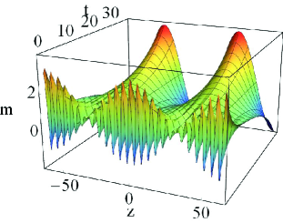
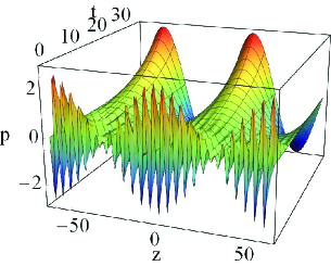
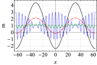
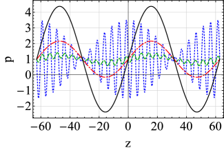
Figure 3: Three-dimensional plots of (a) 1+m1(t,z)+m2(t,z)1subscript𝑚1𝑡𝑧subscript𝑚2𝑡𝑧1+m_{1}(t,z)+m_{2}(t,z) and (b) p1(t,z)+p2(t,z)subscript𝑝1𝑡𝑧subscript𝑝2𝑡𝑧p_{1}(t,z)+p_{2}(t,z), given by Eqs. (2.65), (2.66), (2.71), and (2.72) with N=2,a1=a2=1,k1=1.3,k2=1.2,φ1=φ2=0formulae-sequenceformulae-sequence𝑁2subscript𝑎1subscript𝑎21formulae-sequencesubscript𝑘11.3formulae-sequencesubscript𝑘21.2subscript𝜑1subscript𝜑20N=2,\;a_{1}=a_{2}=1,\;k_{1}=1.3,\;k_{2}=1.2,\;\varphi_{1}=\varphi_{2}=0. Snapshots of (c) 1+m1(t,z)+m2(t,z)1subscript𝑚1𝑡𝑧subscript𝑚2𝑡𝑧1+m_{1}(t,z)+m_{2}(t,z) and (d) p1(t,z)+p2(t,z)subscript𝑝1𝑡𝑧subscript𝑝2𝑡𝑧p_{1}(t,z)+p_{2}(t,z) at t=0𝑡0t=0 (blue dotted), t=8𝑡8t=8 (green dashed), t=28𝑡28t=28 (red dot-dashed), and t=40𝑡40t=40 (black solid).

2.3.3 Notes on Gregory-Laflamme instability

Let us consider the meaning to investigate the higher-order perturbations from the stability point of view. The asymptotically flat black brane we consider here is essentially unstable. Namely, as seen in Sec. 2.3.1, if the initial perturbation contains any mode of which wave number kn(1,1){0}subscript𝑘𝑛110k_{n}\in(-1,1)\setminus\{0\}, such a mode grows unboundedly. However, we consider the black brane in the large-D𝐷D limit, namely, above the critical dimension [5]. Thus, the GL instability initially grows but it gradually damps in non-linear regimes, and eventually the horizon converges to non-uniform configuration [4].

It is pointed out that the second-order perturbation cannot stabilize the first-order instability because the first-order perturbation is treated as the fixed background, which appears as the source term, when we solve the second order. Nevertheless, one might expect if there appears the sign of the convergence to the non-uniform horizon at the second order. Although such a sign can appear at the second order, we cannot catch the sign in the result (2.71) and (2.72) unfortunately.

On the other hand, a black brane that is linearly stable can become unstable at the second order. If the initial perturbation does not contain any unstable mode, the initial perturbation will damp exponentially at linear level, as seen in the results of Sec. 2.3.1. However, the second-order perturbation involves various time dependence as seen in Eqs. (2.73) and (2.74). In order to see directly this situation, let us focus on a simple case as follow.

Suppose that the initial perturbation is the superposition of two modes k1subscript𝑘1k_{1} and k2subscript𝑘2k_{2} both of which are stable modes, k1>k2>1subscript𝑘1subscript𝑘21k_{1}>k_{2}>1. In addition, assume that their difference is smaller than unity, k1k2(0,1)subscript𝑘1subscript𝑘201k_{1}-k_{2}\in(0,1). In this case, the term of C21(+)()cos[(k1k2)z+(φ1φ2)]subscriptsuperscript𝐶21subscript𝑘1subscript𝑘2𝑧subscript𝜑1subscript𝜑2C^{(+)(-)}_{21}\cos[(k_{1}-k_{2})z+(\varphi_{1}-\varphi_{2})] in Eq. (2.71) includes terms having growing factor es+(k1k2)tsuperscript𝑒subscript𝑠subscript𝑘1subscript𝑘2𝑡e^{s_{+}(k_{1}-k_{2})t}, as seen from Eq. (2.68). Thus, the perturbation does not grow at O(ϵ)𝑂italic-ϵO(\epsilon) but does at O(ϵ2)𝑂superscriptitalic-ϵ2O(\epsilon^{2}).

The above phenomenon is an interesting aspect of the GL instability, which was revealed for the first time by the present non-linear perturbation theory in time domain. It is intuitively understandable. The superposition of the two modes forms the beat. For simplicity, assume a1=a2(0)subscript𝑎1annotatedsubscript𝑎2absent0a_{1}=a_{2}\;(\neq 0) in Eq. (2.57), then the superposed wave is written as

2a1cos[(k1+k2)z+(φ1+φ2)2]cos[(k1k2)z+(φ1φ2)2].2subscript𝑎1subscript𝑘1subscript𝑘2𝑧subscript𝜑1subscript𝜑22subscript𝑘1subscript𝑘2𝑧subscript𝜑1subscript𝜑22\displaystyle 2a_{1}\cos[\frac{(k_{1}+k_{2})z+(\varphi_{1}+\varphi_{2})}{2}]\cos[\frac{(k_{1}-k_{2})z+(\varphi_{1}-\varphi_{2})}{2}]. (2.75)

This exhibits the fast spatial oscillation with the large wave number k1+k22subscript𝑘1subscript𝑘22\frac{k_{1}+k_{2}}{2} which is enveloped by the slow oscillation with the small wave number k1k22subscript𝑘1subscript𝑘22\frac{k_{1}-k_{2}}{2}, which is called the beat phenomenon especially when the difference of the wave numbers is rather small k1k2k1+k2much-less-thansubscript𝑘1subscript𝑘2subscript𝑘1subscript𝑘2k_{1}-k_{2}\ll k_{1}+k_{2}. This slow oscillation is nothing but the origin of the GL instability at the second order. In Fig. 3, we present the three-dimensional plots of m(t,z)=1+m1(t,z)+m2(t,z)𝑚𝑡𝑧1subscript𝑚1𝑡𝑧subscript𝑚2𝑡𝑧m(t,z)=1+m_{1}(t,z)+m_{2}(t,z) and p1(t,z)+p2(t,z)subscript𝑝1𝑡𝑧subscript𝑝2𝑡𝑧p_{1}(t,z)+p_{2}(t,z) and their snapshots at selected moments. One can observe that the beat formed by the superposition of two modes at t=0𝑡0t=0. As soon as the dynamics starts, such an initial wave rapidly damps as predicted by the first-order perturbation. As the time proceeds, however, the waves of which scale is the same order as that of the beat begin to grow and eventually diverge.

3 Asymptotically AdS black branes

In this section, we consider the non-linear perturbation of the asymptotically AdS black branes in the large-D𝐷D limit. The governing equations of motion are almost the same as those in the asymptotically flat case except for a sign of one term. Thus, the formulation of the perturbation theory proceeds completely in parallel with the asymptotically flat case.

What different from the asymptotically flat black brane in the previous section is that the AdS black branes are stable: they are not suffered from the GL instability at least linearly. In addition, the gravitational phenomena in AdS background are interpreted as corresponding phenomena in the dual field theories via the AdS/CFT dictionary, and therefore have much more applications than the asymptotically flat case. In fact, we will apply the result of general perturbation theory to the problem of shock-wave propagation, which has been discussed in the context of AdS/CFT [7], in Secs. 3.3 and 3.4 in addition to the Gaussian wave packet and general superposed sinusoidal waves.

3.1 Perturbation equations and general form of solutions

For the asymptotically AdS neutral black branes in the large-D𝐷D limit of general relativity, the mass and momentum distribution, m(t,z)𝑚𝑡𝑧m(t,z) and p(t,z)𝑝𝑡𝑧p(t,z), obey Eq. (2.1) and the following equation [4, 7] with the domain (2.3),

(tz2)p+zm=z(p2m).subscript𝑡superscriptsubscript𝑧2𝑝subscript𝑧𝑚subscript𝑧superscript𝑝2𝑚\displaystyle(\partial_{t}-\partial_{z}^{2})p+\partial_{z}m=-\partial_{z}(\frac{p^{2}}{m}). (3.1)

Substituting the expansion (2.4) and (2.5) into Eqs. (2.1) and (3.1), we obtain Eq. (2.6) and

p˙p′′+m=ψ,subscript˙𝑝superscriptsubscript𝑝′′superscriptsubscript𝑚subscript𝜓\displaystyle\dot{p}_{\ell}-p_{\ell}^{\prime\prime}+m_{\ell}^{\prime}=\psi_{\ell}, (3.2)

where the source term ψsubscript𝜓\psi_{\ell} is the same as those in the asymptotically Minkowski case, Eqs. (2.8)–(2.11).

Performing the Laplace and Fourier transformation in Eqs. (2.6) and (3.2), we obtain a couple of algebraic equations, which is written as Eq. (2.21) with 𝑨𝑨{\bm{A}} replaced by the following matrix,

𝑫:=(s+k2ikiks+k2).assign𝑫𝑠superscript𝑘2𝑖𝑘𝑖𝑘𝑠superscript𝑘2\displaystyle{\bm{D}}:=\left(\begin{array}[]{cc}s+k^{2}&ik\\ ik&s+k^{2}\\ \end{array}\right). (3.5)

The inverse matrix 𝑫1superscript𝑫1{\bm{D}}^{-1} is decomposed into two parts,

𝑫1=σ=+,1s𝗌σ(k)𝑬σ,superscript𝑫1subscript𝜎1𝑠subscript𝗌𝜎𝑘subscript𝑬𝜎\displaystyle{\bm{D}}^{-1}=\sum_{\sigma=+,-}\frac{1}{s-{\mathsf{s}}_{\sigma}(k)}{\bm{E}}_{\sigma}, (3.6)
𝑬σ:=12(1σ1σ11),assignsubscript𝑬𝜎121𝜎1𝜎11\displaystyle{\bm{E}}_{\sigma}:=\frac{1}{2}\left(\begin{array}[]{cc}1&-\sigma 1\\ -\sigma 1&1\\ \end{array}\right), (3.9)
𝗌σ(k):=k(σik).assignsubscript𝗌𝜎𝑘𝑘𝜎𝑖𝑘\displaystyle{\mathsf{s}}_{\sigma}(k):=k(\sigma i-k). (3.10)

After this decomposition, one can perform the inverse Laplace transformation 1superscript1{\cal L}^{-1} in Eq. (2.29) with 𝑨𝑨{\bm{A}} replaced by 𝑫𝑫{\bm{D}}. Then, the general form of solution is given by

(m(t,z)p(t,z))subscript𝑚𝑡𝑧subscript𝑝𝑡𝑧\displaystyle\left(\begin{array}[]{c}m_{\ell}(t,z)\\ p_{\ell}(t,z)\\ \end{array}\right) =σ=+,𝑬σ(1[e𝗌σ(k)tm¯(0,k)]1[e𝗌σ(k)tp¯(0,k)+e𝗌σ(k)tψ¯(t,k)])absentsubscript𝜎subscript𝑬𝜎superscript1delimited-[]superscript𝑒subscript𝗌𝜎𝑘𝑡subscript¯𝑚0𝑘superscript1delimited-[]superscript𝑒subscript𝗌𝜎𝑘𝑡subscript¯𝑝0𝑘superscript𝑒subscript𝗌𝜎𝑘𝑡subscript¯𝜓𝑡𝑘\displaystyle=\sum_{\sigma=+,-}{\bm{E}}_{\sigma}\left(\begin{array}[]{c}{\cal F}^{-1}[e^{{\mathsf{s}}_{\sigma}(k)t}\bar{m}_{\ell}(0,k)]\\ {\cal F}^{-1}[e^{{\mathsf{s}}_{\sigma}(k)t}\bar{p}_{\ell}(0,k)+e^{{\mathsf{s}}_{\sigma}(k)t}\ast\bar{\psi}_{\ell}(t,k)]\\ \end{array}\right) (3.15)
=σ=+,𝑬σ(1[e𝗌σ(k)t]m(0,z)1[e𝗌σ(k)t]p(0,z)+1[e𝗌σ(k)t]ψ(t,z)).\displaystyle=\sum_{\sigma=+,-}{\bm{E}}_{\sigma}\left(\begin{array}[]{c}{\cal F}^{-1}[e^{{\mathsf{s}}_{\sigma}(k)t}]\star m_{\ell}(0,z)\\ {\cal F}^{-1}[e^{{\mathsf{s}}_{\sigma}(k)t}]\star p_{\ell}(0,z)+{\cal F}^{-1}[e^{{\mathsf{s}}_{\sigma}(k)t}]\star\ast\psi_{\ell}(t,z)\\ \end{array}\right). (3.18)

While it depends on the chosen initial condition which expression between (3.15) and (3.18) is easier to compute, Eq. (3.15) is solely used in the rest of this paper. Using Eq. (3.10), the inverse Fourier transformation of e𝗌σ(k)tsuperscript𝑒subscript𝗌𝜎𝑘𝑡e^{{\mathsf{s}}_{\sigma}(k)t} is easily computed as

1[e𝗌σ(k)t]=14πtexp[(σt+z)24t].superscript1delimited-[]superscript𝑒subscript𝗌𝜎𝑘𝑡14𝜋𝑡superscript𝜎𝑡𝑧24𝑡\displaystyle{\cal F}^{-1}[e^{{\mathsf{s}}_{\sigma}(k)t}]=\frac{1}{\sqrt{4\pi t}}\exp[-\frac{(\sigma t+z)^{2}}{4t}]. (3.19)

This will be useful when one uses expression (3.18).

3.2 Gaussian wave packet

As in Sec. 2.2, we investigate the Gaussian wave packet as the initial perturbation given to the asymptotically AdS black brane. Compared with the full-order numerical solution, the linear-order approximation turns out to be rather accurate approximation in this case.

(a) (b)
Refer to caption Refer to caption
(c) (d)
Refer to caption Refer to caption
Figure 4: Three-dimensional plots of (a) 1+m1(t,z)1subscript𝑚1𝑡𝑧1+m_{1}(t,z) and (b) p1(t,z)subscript𝑝1𝑡𝑧p_{1}(t,z), given by Eq. (3.26) with β=b=1,z0=0formulae-sequence𝛽𝑏1subscript𝑧00\beta=b=1,\;z_{0}=0. The comparison between first-order solution (c) 1+m1(t,z)1subscript𝑚1𝑡𝑧1+m_{1}(t,z) (resp. (d) p1(t,z)subscript𝑝1𝑡𝑧p_{1}(t,z)) and full solution m(t,z)𝑚𝑡𝑧m(t,z) (resp. p(t,z)𝑝𝑡𝑧p(t,z)) obtained by solving Eqs. (2.1) and (3.1) numerically. Snapshots of (c) 1+m1(t,z)1subscript𝑚1𝑡𝑧1+m_{1}(t,z) and (d) p1(t,z)subscript𝑝1𝑡𝑧p_{1}(t,z) at t=0𝑡0t=0 (blue-dashed), t=0.67𝑡0.67t=0.67 (green-solid), t=2.0𝑡2.0t=2.0 (red-solid), and t=10𝑡10t=10 (black-solid). Non-perturbative solutions obtained by solving Eqs. (2.1) and (3.1) numerically are drawn by (green, red, and black) dashed curves too, but can be hardly distinguished from the first-order solutions.

3.2.1 First-order solutions

For the initial perturbation given by the Gaussian wave packet, Eqs. (2.44) and (2.45), one can compute the following quantities

1[e𝗌σ(k)tm¯1(0,k)]superscript1delimited-[]superscript𝑒subscript𝗌𝜎𝑘𝑡subscript¯𝑚10𝑘\displaystyle{\cal F}^{-1}[e^{{\mathsf{s}}_{\sigma}(k)t}\bar{m}_{1}(0,k)] =β2π(b2+2t)exp[t2+(zz0)22(b2+2t)σt(zz0)b2+2t],absent𝛽2𝜋superscript𝑏22𝑡superscript𝑡2superscript𝑧subscript𝑧022superscript𝑏22𝑡𝜎𝑡𝑧subscript𝑧0superscript𝑏22𝑡\displaystyle=\frac{\beta}{\sqrt{2\pi(b^{2}+2t)}}\exp[-\frac{t^{2}+(z-z_{0})^{2}}{2(b^{2}+2t)}-\sigma\frac{t(z-z_{0})}{b^{2}+2t}], (3.20)
1[e𝗌σ(k)tp¯1(0,k)]superscript1delimited-[]superscript𝑒subscript𝗌𝜎𝑘𝑡subscript¯𝑝10𝑘\displaystyle{\cal F}^{-1}[e^{{\mathsf{s}}_{\sigma}(k)t}\bar{p}_{1}(0,k)] =β(zz0+σt)2π(b2+2t)3exp[t2+(zz0)22(b2+2t)σt(zz0)b2+2t].absent𝛽𝑧subscript𝑧0𝜎𝑡2𝜋superscriptsuperscript𝑏22𝑡3superscript𝑡2superscript𝑧subscript𝑧022superscript𝑏22𝑡𝜎𝑡𝑧subscript𝑧0superscript𝑏22𝑡\displaystyle=-\frac{\beta(z-z_{0}+\sigma t)}{\sqrt{2\pi(b^{2}+2t)^{3}}}\exp[-\frac{t^{2}+(z-z_{0})^{2}}{2(b^{2}+2t)}-\sigma\frac{t(z-z_{0})}{b^{2}+2t}]. (3.21)

Substituting these quantities into Eq. (3.15), we obtain the first-order solution,

(m1(t,z)p1(t,z))=β(b2+3t)2(zz0)22π(b2+2t)3exp[t2+(zz0)22(b2+2t)](cosh[t(zz0)b2+2tΞ]sinh[t(zz0)b2+2tΞ]),subscript𝑚1𝑡𝑧subscript𝑝1𝑡𝑧𝛽superscriptsuperscript𝑏23𝑡2superscript𝑧subscript𝑧022𝜋superscriptsuperscript𝑏22𝑡3superscript𝑡2superscript𝑧subscript𝑧022superscript𝑏22𝑡𝑡𝑧subscript𝑧0superscript𝑏22𝑡Ξ𝑡𝑧subscript𝑧0superscript𝑏22𝑡Ξ\displaystyle\left(\begin{array}[]{c}m_{1}(t,z)\\ p_{1}(t,z)\\ \end{array}\right)=\beta\sqrt{\frac{(b^{2}+3t)^{2}-(z-z_{0})^{2}}{2\pi(b^{2}+2t)^{3}}}\exp[-\frac{t^{2}+(z-z_{0})^{2}}{2(b^{2}+2t)}]\left(\begin{array}[]{c}\displaystyle\cosh[\frac{t(z-z_{0})}{b^{2}+2t}-\Xi]\\ \displaystyle\sinh[\frac{t(z-z_{0})}{b^{2}+2t}-\Xi]\\ \end{array}\right), (3.26)

where

coshΞ:=b2+3t(b2+3t)2(zz0)2,sinhΞ:=zz0(b2+3t)2(zz0)2.formulae-sequenceassignΞsuperscript𝑏23𝑡superscriptsuperscript𝑏23𝑡2superscript𝑧subscript𝑧02assignΞ𝑧subscript𝑧0superscriptsuperscript𝑏23𝑡2superscript𝑧subscript𝑧02\displaystyle\cosh\Xi:=\frac{b^{2}+3t}{\sqrt{(b^{2}+3t)^{2}-(z-z_{0})^{2}}},\;\;\;\sinh\Xi:=\frac{z-z_{0}}{\sqrt{(b^{2}+3t)^{2}-(z-z_{0})^{2}}}. (3.27)

Like the diffusion phenomenon of a Gaussian wave packet according to an ordinary diffusion equation, solutions (3.26) have temporal decay factor, which behaves as 1b2+2t1superscript𝑏22𝑡\frac{1}{\sqrt{b^{2}+2t}}, and spatial decay factor exp[(zz0)22(b2+2t)]superscript𝑧subscript𝑧022superscript𝑏22𝑡\exp[-\frac{(z-z_{0})^{2}}{2(b^{2}+2t)}]. What crucially different from the ordinary diffusion is that the solution temporally damps rapidly due to factor exp[t22(b2+2t)]superscript𝑡22superscript𝑏22𝑡\exp[-\frac{t^{2}}{2(b^{2}+2t)}].

Three-dimensional plots of 1+m1(t,z)1subscript𝑚1𝑡𝑧1+m_{1}(t,z) and p1(t,z)subscript𝑝1𝑡𝑧p_{1}(t,z) are presented in Figs. 4(a) and 4(b), respectively. One can observe the fast damping described above. In addition, snapshots of 1+m1(t,z)1subscript𝑚1𝑡𝑧1+m_{1}(t,z) and p1(t,z)subscript𝑝1𝑡𝑧p_{1}(t,z) at selected moments, compared with numerical solutions, are presented in Figs. 4(c) and 4(d), respectively. Compared with the full numerical solutions, which are obtained by directly solving original equations (2.1) and (3.1) with the same initial conditions, i.e., m(0,z)=1+m1(0,z)𝑚0𝑧1subscript𝑚10𝑧m(0,z)=1+m_{1}(0,z) and p(0,z)=p1(0,z)𝑝0𝑧subscript𝑝10𝑧p(0,z)=p_{1}(0,z), one can observe that the first-order solution completely captures the full solution throughout the time domain considered. In other words, the higher-order perturbations are negligible, meaning that the ϵitalic-ϵ\epsilon-expansion Eqs. (2.4) and (2.5) converges rapidly for this example.

3.3 Shock wave

Here, let us consider the step-function like shock as the initial perturbation to the asymptotically AdS black brane. The propagation of this kind of shock is known as the Riemann problem in fluid mechanics. This classic problem attracts attentions recently in relativistic hydrodynamics since it makes us understand the non-equilibrium physics of quantum field theories. See the introduction of Ref. [7] for a brief but nice review for the recent development.

Assume that the black brane is given O(ϵ)𝑂italic-ϵO(\epsilon) perturbation as follows,

m1(0,z)=αsgn(z),p1(0,z)=0,formulae-sequencesubscript𝑚10𝑧𝛼sgn𝑧subscript𝑝10𝑧0\displaystyle m_{1}(0,z)=\alpha\;{\rm sgn}(z),\;\;\;p_{1}(0,z)=0, (3.28)

where α𝛼\alpha is a real constant and sgn denotes the sign function,

sgn(z):={1(z<0)0(z=0)+1(z>0).assignsgn𝑧cases1𝑧00𝑧01𝑧0\displaystyle{\rm sgn}(z):=\begin{cases}-1&(z<0)\\ 0&(z=0)\\ +1&(z>0)\\ \end{cases}. (3.29)

The assumption that p1subscript𝑝1p_{1} initially vanishes is adopted to reproduce a situation considered in Ref. [7] (see the left panel of Fig. 5 in [7]). The Fourier transformation of the above initial conditions are

m¯1(0,k)=2iαk,p¯1(0,k)=0.formulae-sequencesubscript¯𝑚10𝑘2𝑖𝛼𝑘subscript¯𝑝10𝑘0\displaystyle\bar{m}_{1}(0,k)=-\frac{2i\alpha}{k},\;\;\;\bar{p}_{1}(0,k)=0. (3.30)
(a) (b)
Refer to caption Refer to caption
(c) (d)
Refer to caption Refer to caption
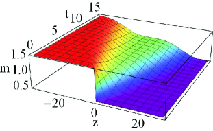
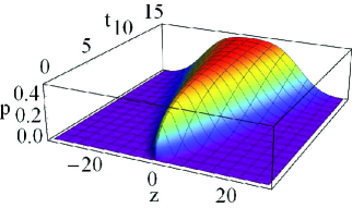
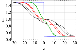
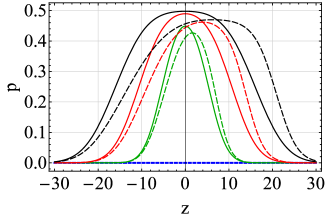
Figure 5: Three dimensional plots of (a) 1+m1(t,z)1subscript𝑚1𝑡𝑧1+m_{1}(t,z) and (b) p1(t,z)subscript𝑝1𝑡𝑧p_{1}(t,z), given by Eqs. (3.33) and (3.34) with α=1/2𝛼12\alpha=-1/2, respectively. The comparison between first-order solution (c) 1+m1(t,z)1subscript𝑚1𝑡𝑧1+m_{1}(t,z) (resp. (d) p1(t,z)subscript𝑝1𝑡𝑧p_{1}(t,z)) and full-order numerical solution m(t,z)𝑚𝑡𝑧m(t,z) (resp. p(t,z)𝑝𝑡𝑧p(t,z)), obtained by solving Eqs. (2.1) and (3.1). The blue-dashed curve represents initial configuration m(0,z)𝑚0𝑧m(0,z) (resp. p(0,z)𝑝0𝑧p(0,z)). The green, red, and black solid curves represent the first-order solutions at t=7.3𝑡7.3t=7.3, 141414, and 222222, respectively. The (green, red, and black) dashed curve represents the full numerical solution at the corresponding time.

3.3.1 First-order solutions

Using Eqs. (3.10) and (3.30), one obtains

1[e𝗌σ(k)tm¯1(0,k)]=αerf(σt+z2t),1[e𝗌σ(k)tp¯1(0,k)]=0,formulae-sequencesuperscript1delimited-[]superscript𝑒subscript𝗌𝜎𝑘𝑡subscript¯𝑚10𝑘𝛼erf𝜎𝑡𝑧2𝑡superscript1delimited-[]superscript𝑒subscript𝗌𝜎𝑘𝑡subscript¯𝑝10𝑘0\displaystyle{\cal F}^{-1}[e^{{\mathsf{s}}_{\sigma}(k)t}\bar{m}_{1}(0,k)]=\alpha\;{\rm erf}(\frac{\sigma t+z}{2\sqrt{t}}),\;\;\;{\cal F}^{-1}[e^{{\mathsf{s}}_{\sigma}(k)t}\bar{p}_{1}(0,k)]=0, (3.31)

where erf(x):=2π0xex2𝑑xassignerf𝑥2𝜋superscriptsubscript0𝑥superscript𝑒superscript𝑥2differential-d𝑥{\rm erf}(x):=\frac{2}{\sqrt{\pi}}\int_{0}^{x}e^{-x^{2}}dx is the Gauss error function. Here, we have used the following formula

ea(kib)2k𝑑k=iπeab2erf(ab2),a>0,b.formulae-sequencesuperscriptsubscriptsuperscript𝑒𝑎superscript𝑘𝑖𝑏2𝑘differential-d𝑘𝑖𝜋superscript𝑒𝑎superscript𝑏2erf𝑎superscript𝑏2formulae-sequence𝑎0𝑏\displaystyle\int_{-\infty}^{\infty}\frac{e^{-a(k-ib)^{2}}}{k}dk=i\pi e^{ab^{2}}{\rm erf}(\sqrt{a}b^{2}),\;\;\;a>0,\;b\in{\mathbb{R}}. (3.32)

Substituting Eq. (3.31) into Eq. (3.15), one obtains the first-order solution,

m1(t,z)subscript𝑚1𝑡𝑧\displaystyle m_{1}(t,z) =α2[erf(t+z2t)erf(tz2t)],absent𝛼2delimited-[]erf𝑡𝑧2𝑡erf𝑡𝑧2𝑡\displaystyle=\frac{\alpha}{2}\left[{\rm erf}(\frac{t+z}{2\sqrt{t}})-{\rm erf}(\frac{t-z}{2\sqrt{t}})\right], (3.33)
p1(t,z)subscript𝑝1𝑡𝑧\displaystyle p_{1}(t,z) =α2[erf(tz2t)+erf(t+z2t)].absent𝛼2delimited-[]erf𝑡𝑧2𝑡erf𝑡𝑧2𝑡\displaystyle=-\frac{\alpha}{2}\left[{\rm erf}(\frac{t-z}{2\sqrt{t}})+{\rm erf}(\frac{t+z}{2\sqrt{t}})\right]. (3.34)

Using the fact that the Gauss error function is an odd function, one can immediately show that m1(t,z)=m1(t,z)subscript𝑚1𝑡𝑧subscript𝑚1𝑡𝑧m_{1}(t,-z)=-m_{1}(t,z) and p1(t,z)=p1(t,z)subscript𝑝1𝑡𝑧subscript𝑝1𝑡𝑧p_{1}(t,-z)=p_{1}(t,z) hold. Namely, m1(t,z)subscript𝑚1𝑡𝑧m_{1}(t,z) and p1(t,z)subscript𝑝1𝑡𝑧p_{1}(t,z) are spatially odd and even functions, respectively.

In Fig. 5, three-dimensional plots of 1+m1(t,z)1subscript𝑚1𝑡𝑧1+m_{1}(t,z) and p1(t,z)subscript𝑝1𝑡𝑧p_{1}(t,z), where the parameter is chosen as α=1/2𝛼12\alpha=-1/2, and their snapshots at selected moments are presented, compared with the non-perturbative numerical solutions obtained by directly solving Eqs. (2.1) and (3.1) with the initial condition similar to Eq. (3.28). Since the sign function is difficult to treat in numerical computations, we replace sgn(z)sgn𝑧{\rm sgn}(z) by tanh(cz)𝑐𝑧\tanh(cz) with a large positive number c𝑐c (say, c=50𝑐50c=50), based on the fact that limc+tanh(cz)=sgn(z)subscript𝑐𝑐𝑧sgn𝑧\lim_{c\to+\infty}\tanh(cz)={\rm sgn}(z).

In Fig. 5, one can see that as soon as the dynamics begins, the discontinuity separates into two shock fronts moving to left and right, where the former and latter are called the rarefaction wave and shock wave, respectively [7]. The point is that the rarefaction and shock is interpolated by an expanding plateau region with a non-zero constant flux, called the non-equilibrium steady state (NESS).

While it is interesting that we obtained the semi-analytic results (3.33) and (3.34) describing the shock propagation and NESS, they are not satisfactory from some viewpoints. In Fig. 5, one can observe that the full solution becomes asymmetric with respect to zz𝑧𝑧z\to-z, though the linear solutions (3.33) and (3.34) continue to be symmetric. Thus, for example, the value of m𝑚m at the NESS, which is always unity at O(ϵ)𝑂italic-ϵO(\epsilon), deviates between the first order and full solutions. These suggest that the higher-order perturbations are necessary to fill the above gaps. It seems impossible, however, to obtain the second-order solutions analytically since the first-order solution involves the error function. Thus, we will return to the Riemann problem in the next section as the example of the superposed sinusoidal waves.

3.4 Superposed sinusoidal waves

We consider the initial condition which is the superposition of sinusoidal waves like Eqs. (2.57)–(2.59). For later purpose, however, let us assume the O(ϵ)𝑂italic-ϵO(\epsilon) initial momentum vanishes

p1(0,z)=0,subscript𝑝10𝑧0\displaystyle p_{1}(0,z)=0, (3.35)

which is assumed instead of Eq. (2.58). The first- and second-order solutions satisfying initial conditions (2.57)–(2.59) are presented in Appendix A.

3.4.1 First-order solutions

For the initial perturbation which is the superposition of sinusoidal waves (2.57) and (3.35), we obtain

1[e𝗌σ(k)tm¯1(0,k)]=12n=1Nan[e𝗌σ(kn)tei(knz+φn)+e𝗌σ(kn)tei(knz+φn)],superscript1delimited-[]superscript𝑒subscript𝗌𝜎𝑘𝑡subscript¯𝑚10𝑘12superscriptsubscript𝑛1𝑁subscript𝑎𝑛delimited-[]superscript𝑒subscript𝗌𝜎subscript𝑘𝑛𝑡superscript𝑒𝑖subscript𝑘𝑛𝑧subscript𝜑𝑛superscript𝑒subscript𝗌𝜎subscript𝑘𝑛𝑡superscript𝑒𝑖subscript𝑘𝑛𝑧subscript𝜑𝑛\displaystyle{\cal F}^{-1}[e^{{\mathsf{s}}_{\sigma}(k)t}\bar{m}_{1}(0,k)]=\frac{1}{2}\sum_{n=1}^{N}a_{n}[e^{{\mathsf{s}}_{\sigma}(k_{n})t}e^{i(k_{n}z+\varphi_{n})}+e^{{\mathsf{s}}_{-\sigma}(k_{n})t}e^{-i(k_{n}z+\varphi_{n})}], (3.36)
1[e𝗌σ(k)tp¯1(0,k)]=0,superscript1delimited-[]superscript𝑒subscript𝗌𝜎𝑘𝑡subscript¯𝑝10𝑘0\displaystyle{\cal F}^{-1}[e^{{\mathsf{s}}_{\sigma}(k)t}\bar{p}_{1}(0,k)]=0, (3.37)

where we have used 𝗌σ(k)=𝗌σ(k)subscript𝗌𝜎𝑘subscript𝗌𝜎𝑘{\mathsf{s}}_{\sigma}(-k)={\mathsf{s}}_{-\sigma}(k). Substituting these results into Eq. (3.15) and using the concrete form of the dispersion relation 𝗌σ(k)subscript𝗌𝜎𝑘{\mathsf{s}}_{\sigma}(k), we obtain the first-order solutions,

m1(t,z)=subscript𝑚1𝑡𝑧absent\displaystyle m_{1}(t,z)= n=1Nanekn2tcos(knt)cos(knz+φn),superscriptsubscript𝑛1𝑁subscript𝑎𝑛superscript𝑒superscriptsubscript𝑘𝑛2𝑡subscript𝑘𝑛𝑡subscript𝑘𝑛𝑧subscript𝜑𝑛\displaystyle\sum_{n=1}^{N}a_{n}e^{-k_{n}^{2}t}\cos(k_{n}t)\cos(k_{n}z+\varphi_{n}), (3.38)
p1(t,z)=subscript𝑝1𝑡𝑧absent\displaystyle p_{1}(t,z)= n=1Nanekn2tsin(knt)sin(knz+φn).superscriptsubscript𝑛1𝑁subscript𝑎𝑛superscript𝑒superscriptsubscript𝑘𝑛2𝑡subscript𝑘𝑛𝑡subscript𝑘𝑛𝑧subscript𝜑𝑛\displaystyle\sum_{n=1}^{N}a_{n}e^{-k_{n}^{2}t}\sin(k_{n}t)\sin(k_{n}z+\varphi_{n}). (3.39)

These results (3.38) and (3.39) tell us that the initial perturbation necessarily exhibits the damped oscillation for arbitrary non-zero wave number kn{0}subscript𝑘𝑛0k_{n}\in{\mathbb{R}}\setminus\{0\} (n=1,2,,N𝑛12𝑁n=1,2,\cdots,N), showing the black brane to be linearly stable.

3.4.2 Second-order solutions

Since we assume that the initial values vanish at O(ϵ2)𝑂superscriptitalic-ϵ2O(\epsilon^{2}), m2(0,z)=p2(0,z)=0subscript𝑚20𝑧subscript𝑝20𝑧0m_{2}(0,z)=p_{2}(0,z)=0, we see from Eq. (3.15) that what to compute is the inverse Fourier transformation of the convolution between e𝗌σ(k)tsuperscript𝑒subscript𝗌𝜎𝑘𝑡e^{{\mathsf{s}}_{\sigma}(k)t} and the Fourier spectrum of source term ψ¯2(t,k)subscript¯𝜓2𝑡𝑘\bar{\psi}_{2}(t,k). Using Eqs. (2.10) and (3.39), such a quantity is computed and written down in a simple form as

1[e𝗌σ(k)t\displaystyle{\cal F}^{-1}[e^{{\mathsf{s}}_{\sigma}(k)t}\ast ψ¯2(t,k)]=i8n=1Nn=1Nanankn\displaystyle\bar{\psi}_{2}(t,k)]=-\frac{i}{8}\sum_{n=1}^{N}\sum_{n^{\prime}=1}^{N}a_{n}a_{n^{\prime}}k_{n^{\prime}}
×(Fnn(σ)(+)ei[(kn+kn)z+(φn+φn)]+Fnn(σ)()ei[(knkn)z+(φnφn)]\displaystyle\times\Big{(}F_{nn^{\prime}}^{(\sigma)(+)}e^{i[(k_{n}+k_{n^{\prime}})z+(\varphi_{n}+\varphi_{n^{\prime}})]}+F_{nn^{\prime}}^{(\sigma)(-)}e^{i[(k_{n}-k_{n^{\prime}})z+(\varphi_{n}-\varphi_{n^{\prime}})]}
Fnn(σ)()ei[(knkn)z+(φnφn)]Fnn(σ)(+)ei[(kn+kn)z+(φn+φn)])\displaystyle-F_{nn^{\prime}}^{(-\sigma)(-)}e^{-i[(k_{n}-k_{n^{\prime}})z+(\varphi_{n}-\varphi_{n^{\prime}})]}-F_{nn^{\prime}}^{(-\sigma)(+)}e^{-i[(k_{n}+k_{n^{\prime}})z+(\varphi_{n}+\varphi_{n^{\prime}})]}\Big{)} (3.40)

by defining a function of time,

Fnn(σ)(σ):=assignsuperscriptsubscript𝐹𝑛superscript𝑛𝜎superscript𝜎absent\displaystyle F_{nn^{\prime}}^{(\sigma)(\sigma^{\prime})}:= 1𝗌+(kn)+𝗌+(kn)𝗌σ(kn+σkn)(e[𝗌+(kn)+𝗌+(kn)]te𝗌σ(kn+σkn)t)1subscript𝗌subscript𝑘𝑛subscript𝗌subscript𝑘superscript𝑛subscript𝗌𝜎subscript𝑘𝑛superscript𝜎subscript𝑘superscript𝑛superscript𝑒delimited-[]subscript𝗌subscript𝑘𝑛subscript𝗌subscript𝑘superscript𝑛𝑡superscript𝑒subscript𝗌𝜎subscript𝑘𝑛superscript𝜎subscript𝑘superscript𝑛𝑡\displaystyle\frac{1}{{\mathsf{s}}_{+}(k_{n})+{\mathsf{s}}_{+}(k_{n^{\prime}})-{\mathsf{s}}_{\sigma}(k_{n}+\sigma^{\prime}k_{n^{\prime}})}(e^{[{\mathsf{s}}_{+}(k_{n})+{\mathsf{s}}_{+}(k_{n^{\prime}})]t}-e^{{\mathsf{s}}_{\sigma}(k_{n}+\sigma^{\prime}k_{n^{\prime}})t})
\displaystyle- 1𝗌+(kn)+𝗌(kn)𝗌σ(kn+σkn)(e[𝗌+(kn)+𝗌(kn)]te𝗌σ(kn+σkn)t)1subscript𝗌subscript𝑘𝑛subscript𝗌subscript𝑘superscript𝑛subscript𝗌𝜎subscript𝑘𝑛superscript𝜎subscript𝑘superscript𝑛superscript𝑒delimited-[]subscript𝗌subscript𝑘𝑛subscript𝗌subscript𝑘superscript𝑛𝑡superscript𝑒subscript𝗌𝜎subscript𝑘𝑛superscript𝜎subscript𝑘superscript𝑛𝑡\displaystyle\frac{1}{{\mathsf{s}}_{+}(k_{n})+{\mathsf{s}}_{-}(k_{n^{\prime}})-{\mathsf{s}}_{\sigma}(k_{n}+\sigma^{\prime}k_{n^{\prime}})}(e^{[{\mathsf{s}}_{+}(k_{n})+{\mathsf{s}}_{-}(k_{n^{\prime}})]t}-e^{{\mathsf{s}}_{\sigma}(k_{n}+\sigma^{\prime}k_{n^{\prime}})t})
\displaystyle- 1𝗌(kn)+𝗌+(kn)𝗌σ(kn+σkn)(e[𝗌(kn)+𝗌+(kn)]te𝗌σ(kn+σkn)t)1subscript𝗌subscript𝑘𝑛subscript𝗌subscript𝑘superscript𝑛subscript𝗌𝜎subscript𝑘𝑛superscript𝜎subscript𝑘superscript𝑛superscript𝑒delimited-[]subscript𝗌subscript𝑘𝑛subscript𝗌subscript𝑘superscript𝑛𝑡superscript𝑒subscript𝗌𝜎subscript𝑘𝑛superscript𝜎subscript𝑘superscript𝑛𝑡\displaystyle\frac{1}{{\mathsf{s}}_{-}(k_{n})+{\mathsf{s}}_{+}(k_{n^{\prime}})-{\mathsf{s}}_{\sigma}(k_{n}+\sigma^{\prime}k_{n^{\prime}})}(e^{[{\mathsf{s}}_{-}(k_{n})+{\mathsf{s}}_{+}(k_{n^{\prime}})]t}-e^{{\mathsf{s}}_{\sigma}(k_{n}+\sigma^{\prime}k_{n^{\prime}})t})
+\displaystyle+ 1𝗌(kn)+𝗌(kn)𝗌σ(kn+σkn)(e[𝗌(kn)+𝗌(kn)]te𝗌σ(kn+σkn)t).1subscript𝗌subscript𝑘𝑛subscript𝗌subscript𝑘superscript𝑛subscript𝗌𝜎subscript𝑘𝑛superscript𝜎subscript𝑘superscript𝑛superscript𝑒delimited-[]subscript𝗌subscript𝑘𝑛subscript𝗌subscript𝑘superscript𝑛𝑡superscript𝑒subscript𝗌𝜎subscript𝑘𝑛superscript𝜎subscript𝑘superscript𝑛𝑡\displaystyle\frac{1}{{\mathsf{s}}_{-}(k_{n})+{\mathsf{s}}_{-}(k_{n^{\prime}})-{\mathsf{s}}_{\sigma}(k_{n}+\sigma^{\prime}k_{n^{\prime}})}(e^{[{\mathsf{s}}_{-}(k_{n})+{\mathsf{s}}_{-}(k_{n^{\prime}})]t}-e^{{\mathsf{s}}_{\sigma}(k_{n}+\sigma^{\prime}k_{n^{\prime}})t}). (3.41)

Substituting the above result (3.40) into Eq. (3.15), we have the second-order solutions as

m2(t,z)=i8n=1nn=1Nanankn([\displaystyle m_{2}(t,z)=\frac{i}{8}\sum_{n=1}^{n}\sum_{n^{\prime}=1}^{N}a_{n}a_{n^{\prime}}k_{n^{\prime}}\Big{(}[ Fnn(+)(+)Fnn()(+)]cos[(kn+kn)z+(φn+φn)]\displaystyle F_{nn^{\prime}}^{(+)(+)}-F_{nn^{\prime}}^{(-)(+)}]\cos[(k_{n}+k_{n^{\prime}})z+(\varphi_{n}+\varphi_{n^{\prime}})]
+\displaystyle+ [Fnn(+)()Fnn()()]cos[(knkn)z+(φnφn)]),\displaystyle[F_{nn^{\prime}}^{(+)(-)}-F_{nn^{\prime}}^{(-)(-)}]\cos[(k_{n}-k_{n^{\prime}})z+(\varphi_{n}-\varphi_{n^{\prime}})]\Big{)}, (3.42)
p2(t,z)=18n=1nn=1Nanankn([\displaystyle p_{2}(t,z)=\frac{1}{8}\sum_{n=1}^{n}\sum_{n^{\prime}=1}^{N}a_{n}a_{n^{\prime}}k_{n^{\prime}}\Big{(}[ Fnn(+)(+)+Fnn()(+)]sin[(kn+kn)z+(φn+φn)]\displaystyle F_{nn^{\prime}}^{(+)(+)}+F_{nn^{\prime}}^{(-)(+)}]\sin[(k_{n}+k_{n^{\prime}})z+(\varphi_{n}+\varphi_{n^{\prime}})]
+\displaystyle+ [Fnn(+)()+Fnn()()]sin[(knkn)z+(φnφn)]).\displaystyle[F_{nn^{\prime}}^{(+)(-)}+F_{nn^{\prime}}^{(-)(-)}]\sin[(k_{n}-k_{n^{\prime}})z+(\varphi_{n}-\varphi_{n^{\prime}})]\Big{)}. (3.43)

Note that m(t,z)=1+m1(t,z)+m2(t,z)𝑚𝑡𝑧1subscript𝑚1𝑡𝑧subscript𝑚2𝑡𝑧m(t,z)=1+m_{1}(t,z)+m_{2}(t,z) and p(t,z)=p1(t,z)+p2(t,z)𝑝𝑡𝑧subscript𝑝1𝑡𝑧subscript𝑝2𝑡𝑧p(t,z)=p_{1}(t,z)+p_{2}(t,z) with Eqs. (3.38), (3.39), (3.42), and (3.43), represent O(ϵ2)𝑂superscriptitalic-ϵ2O(\epsilon^{2}) approximate time evolution of the initial perturbation, which takes the form of superposed sinusoidal waves (2.57), (3.35), and (2.59). These approximate solutions are rather general in the sense that initial condition (2.57) is general.

Since the initial perturbations are assumed to vanish at O(ϵ2)𝑂superscriptitalic-ϵ2O(\epsilon^{2}), m2(0,z)=p2(0,z)=0subscript𝑚20𝑧subscript𝑝20𝑧0m_{2}(0,z)=p_{2}(0,z)=0, the above solutions contain only the contribution from the source term ψ2=2p1p1subscript𝜓22subscript𝑝1superscriptsubscript𝑝1\psi_{2}=-2p_{1}p_{1}^{\prime}. If one prepares for non-vanishing initial conditions at the second order, its contribution is simply added to the above solution, but such a contribution will exhibit no interesting behavior since it has the time dependence similar to that in O(ϵ)𝑂italic-ϵO(\epsilon) solution.

3.4.3 Shock wave

(a) (b)
Refer to caption Refer to caption
(c) (d)
Refer to caption Refer to caption
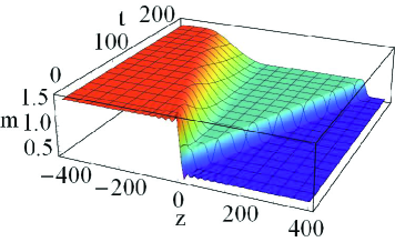
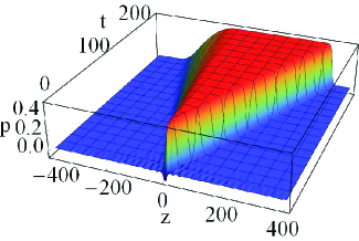
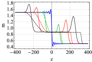
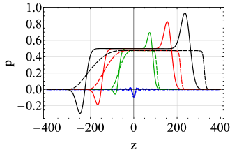
Figure 6: Three-dimensional plots of full-order numerical solution (a) m(t,z)𝑚𝑡𝑧m(t,z) and (b) p(t,z)𝑝𝑡𝑧p(t,z), obtained by solving Eqs. (2.1) and (3.1) with initial condition Eq. (3.29) where sgn(z)sgn𝑧{\rm sgn}(z) is replaced by finite Fourier series of sgnL(z)subscriptsgn𝐿𝑧{\rm sgn}_{L}(z) given by Eqs. (3.45)–(3.47). The comparison between second-order solution (c) 1+m1(t,z)+m2(t,z)1subscript𝑚1𝑡𝑧subscript𝑚2𝑡𝑧1+m_{1}(t,z)+m_{2}(t,z) (resp. (d) p1(t,z)+p2(t,z)subscript𝑝1𝑡𝑧subscript𝑝2𝑡𝑧p_{1}(t,z)+p_{2}(t,z)) and full-order numerical solution m(t,z)𝑚𝑡𝑧m(t,z) (resp. p(t,z)𝑝𝑡𝑧p(t,z)), obtained by solving Eqs. (2.1) and (3.1). The blue-dashed curve represents initial configuration m(0,z)𝑚0𝑧m(0,z) (resp. p(0,z)𝑝0𝑧p(0,z)). The green, red, and black solid curves represent the second-order solutions at t=83.3𝑡83.3t=83.3, 167167167, and 250250250, respectively. The (green, red, and black) dashed curve represents the full numerical solution at the corresponding time.

We re-investigate the Riemann problem in Sec. 3.3, by choosing appropriate parameters (an,kn,φn)subscript𝑎𝑛subscript𝑘𝑛subscript𝜑𝑛(a_{n},k_{n},\varphi_{n}) in initial condition (2.57). In order to do so, the sign function, sgn(z)sgn𝑧{\rm sgn}(z), in initial condition (3.28) is replaced by the following function,

sgnL(z)={1(L<z<0)0(z=0)+1(0<z<L),subscriptsgn𝐿𝑧cases1𝐿𝑧00𝑧010𝑧𝐿\displaystyle{\rm sgn}_{L}(z)=\begin{cases}-1&(-L<z<0)\\ 0&(z=0)\\ +1&(0<z<L)\\ \end{cases}, (3.44)

where L𝐿L is a positive constant and the periodic extension to entire {\mathbb{R}} with period 2L2𝐿2L is assumed. Since this function has the following Fourier series expansion,

sgnL(z)=n=14(2n1)πsin[(2n1)πLz],subscriptsgn𝐿𝑧superscriptsubscript𝑛142𝑛1𝜋2𝑛1𝜋𝐿𝑧\displaystyle{\rm sgn}_{L}(z)=\sum_{n=1}^{\infty}\frac{4}{(2n-1)\pi}\sin[\frac{(2n-1)\pi}{L}z], (3.45)

the parameters in initial condition (2.57) should be

an=4(2n1)π,kn=(2n1)πL,θn=π2formulae-sequencesubscript𝑎𝑛42𝑛1𝜋formulae-sequencesubscript𝑘𝑛2𝑛1𝜋𝐿subscript𝜃𝑛𝜋2\displaystyle a_{n}=\frac{4}{(2n-1)\pi},\;\;\;k_{n}=\frac{(2n-1)\pi}{L},\;\;\;\theta_{n}=-\frac{\pi}{2} (3.46)

for n=1,2,,N𝑛12𝑁n=1,2,\cdots,\;N with the limit N𝑁N\to\infty. Taking large L𝐿L and focusing on the spatial region around the center z=0𝑧0z=0, there must be no difference in the dynamics during a finite interval of time between ones using sgn(z)sgn𝑧{\rm sgn}(z) and sgnL(z)subscriptsgn𝐿𝑧{\rm sgn}_{L}(z), due to the (non-relativistic) causality encoded in the equations of motion.

In Figs. 6(a) and 6(b), we present the three-dimensional plots of full-order numerical solutions of m(t,z)𝑚𝑡𝑧m(t,z) and p(t,z)𝑝𝑡𝑧p(t,z), respectively, starting from the initial condition m(0,z)=1+m1(0,z)𝑚0𝑧1subscript𝑚10𝑧m(0,z)=1+m_{1}(0,z) and p(0,z)=0𝑝0𝑧0p(0,z)=0, where m1(0,z)subscript𝑚10𝑧m_{1}(0,z) is given by Eqs. (2.57) and (3.46). The rest parameters and the cutoff of N𝑁N are chosen as follow,

α=12,L=1000,N=45.formulae-sequence𝛼12formulae-sequence𝐿1000𝑁45\displaystyle\alpha=-\frac{1}{2},\;\;\;L=1000,\;\;\;N=45. (3.47)

In Figs. 6(c) and 6(d), we compare these full solutions with the second-order solutions, i.e., 1+m1(t,z)+m2(t,z)1subscript𝑚1𝑡𝑧subscript𝑚2𝑡𝑧1+m_{1}(t,z)+m_{2}(t,z) and p1(t,z)+p2(t,z)subscript𝑝1𝑡𝑧subscript𝑝2𝑡𝑧p_{1}(t,z)+p_{2}(t,z) provided by Eqs. (3.38), (3.39), (3.42), and (3.43) with initial conditions given by (2.57), (3.46), and (3.47).

Unlike the O(ϵ)𝑂italic-ϵO(\epsilon) approximation in Sec. 3.3, the O(ϵ2)𝑂superscriptitalic-ϵ2O(\epsilon^{2}) approximation presented here captures the spatially asymmetric features under the reflection zz𝑧𝑧z\to-z of full solution. Furthermore, the error of values of m𝑚m and p𝑝p at the plateau of NESS between the O(ϵ2)𝑂superscriptitalic-ϵ2O(\epsilon^{2}) solution and full solutions are within a few percent (1.2%percent1.21.2\% and 5.0%percent5.05.0\% for m𝑚m and p𝑝p, respectively, for the above choice of parameters), which were inadequately large for the O(ϵ)𝑂italic-ϵO(\epsilon) approximation in Sec. 3.3. This is by virtue of the second-order solutions, which appropriately take into account the ‘back-reaction’ of the first-order solution through the source term.

Due to the Gibbs phenomenon, there appears the oscillation near the jump in the initial shock. Such oscillations stem from the artificial cutoff of the Fourier series expansion. As the time proceeds, the ‘horns’ as the remnant of Gibbs oscillations can be observed to propagate near the front of rarefaction and shock waves, and to be amplified. This artifact due to the cutoff will not be a problem when one treats the solution exactly.

4 Conclusion

In the large-D𝐷D(dimension) limit of general relativity, the Einstein equations describing the horizon dynamics of asymptotically flat (resp. AdS) black branes are written in the form of coupled diffusion equations (2.1) and (2.2) (resp. (2.1) and (3.1)) [4, 7]. While these equations are much simpler than the original Einstein equations, there is a non-linear term, making it difficult to solve exactly. Therefore, we have formulated the perturbation theory in this paper making it possible to obtain analytic results on the black-brane dynamics.

The metric functions m(t,z)𝑚𝑡𝑧m(t,z) and p(t,z)𝑝𝑡𝑧p(t,z), which represent the mass and momentum distributions in the direction of horizon z𝑧z, respectively, were expanded around a uniform black-brane solution with formal small parameter ϵitalic-ϵ\epsilon as Eqs. (2.4) and (2.5). Then, the perturbative equations of motion were obtained, and solved order by order using the Laplace and Fourier transformation with respect to t𝑡t and z𝑧z, respectively. As the result, the general form of solutions m(t,z)subscript𝑚𝑡𝑧m_{\ell}(t,z) and p(t,z)subscript𝑝𝑡𝑧p_{\ell}(t,z) in the flat (resp. AdS) background were obtained (2.39) (resp. (3.15)), in which the inverse Fourier transformation of initial spectra m¯(0,k)subscript¯𝑚0𝑘\bar{m}_{\ell}(0,k) and p¯(0,k)subscript¯𝑝0𝑘\bar{p}_{\ell}(0,k), and the spectrum of source term ψ¯(t,k)subscript¯𝜓𝑡𝑘\bar{\psi}_{\ell}(t,k), being a polynomial of lower-order perturbations, were left to be computed.

As the example of initial conditions of perturbation, the Gaussian wave packet was considered for both the asymptotically flat and AdS black branes in Secs. 2.2 and 3.2, respectively, and the first-order solutions were written down explicitly. The resulting dynamics from this initial condition was not surprising itself. Namely, the wave pack grows and damps rapidly for the asymptotically flat and AdS black branes, respectively, which is expected from their known stability. A remarkable point revealed by this example is that the first-order solution captures the features of full-order solution rather accurately even for a finite amplitude. Thus, the convergence of expansion by ϵitalic-ϵ\epsilon (i.e., amplitude) is rather rapid and can be used for finite-amplitude perturbations for a certain class of problems.

Only for the asymptotically AdS black brane, the step-function like initial condition was considered in order to investigate the shock propagation in Sec. 3.3, and the first-order solution was explicitly written down. While the solution captures the emergence and propagation of NESS (non-equilibrium steady state) qualitatively, the first-order solution is not enough to reproduce the properties of NESS such as the values of metric functions and asymmetry of the full solution.

The discretely superposed sinusoidal waves, which can be the Fourier series expansion of an arbitrary piecewise continuous periodic function, were considered for both the asymptotically flat and AdS black branes in Secs. 2.3 and 3.4, respectively, and the first- and second-order solutions were written down explicitly. For the black brane in the flat background, the non-trivial feature of GL (Gregory-Laflamme) instability was revealed. Namely, the mode-mode coupling at the second order can make the perturbation grows even if the initial perturbation damps at the first order. For the black brane in the AdS background, the shock propagation considered in Sec. 3.3 was re-investigated. Thanks to the second-order contribution, the values and asymmetric features of the full solution were reproduced, illustrating the usefulness of the formalism in this paper.

There are many things to do by applying and generalizing the formulation presented in this paper. For instance, (i) it would be interesting to investigate further why the sign of convergence to non-uniform black string (NUBS) of asymptotically flat black string does not appear even in the second-order perturbation. (ii) One is able to investigate the various type of shock-wave propagation such as those discussed in Ref. [7] if one slightly changes the ansatz of expansion (2.4) and (2.5), which is straightforward. (iii) Including 1/D1𝐷1/D corrections and charges of background black branes [11, 12, 13] would increase the problems to be worked by our formalism.

Acknowledgments

The author would like to thank R. Emparan, R. Suzuki, and K. Tanabe for useful discussion and comments during The Spanish-Portuguese Relativity Meetings held at Lisbon (12–15th, Sep. 2016), and T. Torii during his stay at Akita (12–17th, Feb. 2017). This work was supported by JSPS KAKENHI Grant Number 15K05086.

Appendix A Sinusoidal waves in AdS with p1(0,z)=zm1(0,z)subscript𝑝10𝑧subscript𝑧subscript𝑚10𝑧p_{1}(0,z)=\partial_{z}m_{1}(0,z)

For the initial perturbation to the asymptotically AdS black branes which is the superposition of sinusoidal waves (2.57)–(2.59), we obtain

m1(t,z)=subscript𝑚1𝑡𝑧absent\displaystyle m_{1}(t,z)= 12n=1Nan[(1ikn)e𝗌+(kn)t+(1+ikn)e𝗌(kn)t]cos(knz+φn),12superscriptsubscript𝑛1𝑁subscript𝑎𝑛delimited-[]1𝑖subscript𝑘𝑛superscript𝑒subscript𝗌subscript𝑘𝑛𝑡1𝑖subscript𝑘𝑛superscript𝑒subscript𝗌subscript𝑘𝑛𝑡subscript𝑘𝑛𝑧subscript𝜑𝑛\displaystyle\frac{1}{2}\sum_{n=1}^{N}a_{n}[(1-ik_{n})e^{{\mathsf{s}}_{+}(k_{n})t}+(1+ik_{n})e^{{\mathsf{s}}_{-}(k_{n})t}]\cos(k_{n}z+\varphi_{n}), (A.1)
p1(t,z)=subscript𝑝1𝑡𝑧absent\displaystyle p_{1}(t,z)= i2n=1Nan[(1ikn)e𝗌+(kn)t(1+ikn)e𝗌(kn)t]sin(knz+φn).𝑖2superscriptsubscript𝑛1𝑁subscript𝑎𝑛delimited-[]1𝑖subscript𝑘𝑛superscript𝑒subscript𝗌subscript𝑘𝑛𝑡1𝑖subscript𝑘𝑛superscript𝑒subscript𝗌subscript𝑘𝑛𝑡subscript𝑘𝑛𝑧subscript𝜑𝑛\displaystyle-\frac{i}{2}\sum_{n=1}^{N}a_{n}[(1-ik_{n})e^{{\mathsf{s}}_{+}(k_{n})t}-(1+ik_{n})e^{{\mathsf{s}}_{-}(k_{n})t}]\sin(k_{n}z+\varphi_{n}). (A.2)

Using the concrete form of the dispersion relation 𝗌σ(k)subscript𝗌𝜎𝑘{\mathsf{s}}_{\sigma}(k), we obtain the following form of first-order solution,

m1(t,z)=subscript𝑚1𝑡𝑧absent\displaystyle m_{1}(t,z)= n=1N1+kn2anekn2tcos(knt+ϑn)cos(knz+φn),superscriptsubscript𝑛1𝑁1superscriptsubscript𝑘𝑛2subscript𝑎𝑛superscript𝑒superscriptsubscript𝑘𝑛2𝑡subscript𝑘𝑛𝑡subscriptitalic-ϑ𝑛subscript𝑘𝑛𝑧subscript𝜑𝑛\displaystyle\sum_{n=1}^{N}\sqrt{1+k_{n}^{2}}a_{n}e^{-k_{n}^{2}t}\cos(k_{n}t+\vartheta_{n})\cos(k_{n}z+\varphi_{n}), (A.3)
p1(t,z)=subscript𝑝1𝑡𝑧absent\displaystyle p_{1}(t,z)= n=1N1+kn2anekn2tsin(knt+ϑn)sin(knz+φn),superscriptsubscript𝑛1𝑁1superscriptsubscript𝑘𝑛2subscript𝑎𝑛superscript𝑒superscriptsubscript𝑘𝑛2𝑡subscript𝑘𝑛𝑡subscriptitalic-ϑ𝑛subscript𝑘𝑛𝑧subscript𝜑𝑛\displaystyle\sum_{n=1}^{N}\sqrt{1+k_{n}^{2}}a_{n}e^{-k_{n}^{2}t}\sin(k_{n}t+\vartheta_{n})\sin(k_{n}z+\varphi_{n}), (A.4)

where

cosϑn:=11+kn2,sinϑn:=kn1+kn2.formulae-sequenceassignsubscriptitalic-ϑ𝑛11superscriptsubscript𝑘𝑛2assignsubscriptitalic-ϑ𝑛subscript𝑘𝑛1superscriptsubscript𝑘𝑛2\displaystyle\cos\vartheta_{n}:=\frac{1}{\sqrt{1+k_{n}^{2}}},\;\;\;\sin\vartheta_{n}:=-\frac{k_{n}}{\sqrt{1+k_{n}^{2}}}. (A.5)

Equations (3.40), (3.42), and (3.43) hold just by replacing Fnn(σ)(σ)superscriptsubscript𝐹𝑛superscript𝑛𝜎superscript𝜎F_{nn^{\prime}}^{(\sigma)(\sigma^{\prime})} for the following F~nn(σ)(σ)superscriptsubscript~𝐹𝑛superscript𝑛𝜎superscript𝜎\tilde{F}_{nn^{\prime}}^{(\sigma)(\sigma^{\prime})},

F~nn(σ)(σ):=assignsuperscriptsubscript~𝐹𝑛superscript𝑛𝜎superscript𝜎absent\displaystyle\tilde{F}_{nn^{\prime}}^{(\sigma)(\sigma^{\prime})}:= (1ikn)(1ikn)𝗌+(kn)+𝗌+(kn)𝗌σ(kn+σkn)(e[𝗌+(kn)+𝗌+(kn)]te𝗌σ(kn+σkn)t)1𝑖subscript𝑘𝑛1𝑖subscript𝑘superscript𝑛subscript𝗌subscript𝑘𝑛subscript𝗌subscript𝑘superscript𝑛subscript𝗌𝜎subscript𝑘𝑛superscript𝜎subscript𝑘superscript𝑛superscript𝑒delimited-[]subscript𝗌subscript𝑘𝑛subscript𝗌subscript𝑘superscript𝑛𝑡superscript𝑒subscript𝗌𝜎subscript𝑘𝑛superscript𝜎subscript𝑘superscript𝑛𝑡\displaystyle\frac{(1-ik_{n})(1-ik_{n^{\prime}})}{{\mathsf{s}}_{+}(k_{n})+{\mathsf{s}}_{+}(k_{n^{\prime}})-{\mathsf{s}}_{\sigma}(k_{n}+\sigma^{\prime}k_{n^{\prime}})}(e^{[{\mathsf{s}}_{+}(k_{n})+{\mathsf{s}}_{+}(k_{n^{\prime}})]t}-e^{{\mathsf{s}}_{\sigma}(k_{n}+\sigma^{\prime}k_{n^{\prime}})t})
\displaystyle- (1ikn)(1+ikn)𝗌+(kn)+𝗌(kn)𝗌σ(kn+σkn)(e[𝗌+(kn)+𝗌(kn)]te𝗌σ(kn+σkn)t)1𝑖subscript𝑘𝑛1𝑖subscript𝑘superscript𝑛subscript𝗌subscript𝑘𝑛subscript𝗌subscript𝑘superscript𝑛subscript𝗌𝜎subscript𝑘𝑛superscript𝜎subscript𝑘superscript𝑛superscript𝑒delimited-[]subscript𝗌subscript𝑘𝑛subscript𝗌subscript𝑘superscript𝑛𝑡superscript𝑒subscript𝗌𝜎subscript𝑘𝑛superscript𝜎subscript𝑘superscript𝑛𝑡\displaystyle\frac{(1-ik_{n})(1+ik_{n^{\prime}})}{{\mathsf{s}}_{+}(k_{n})+{\mathsf{s}}_{-}(k_{n^{\prime}})-{\mathsf{s}}_{\sigma}(k_{n}+\sigma^{\prime}k_{n^{\prime}})}(e^{[{\mathsf{s}}_{+}(k_{n})+{\mathsf{s}}_{-}(k_{n^{\prime}})]t}-e^{{\mathsf{s}}_{\sigma}(k_{n}+\sigma^{\prime}k_{n^{\prime}})t})
\displaystyle- (1+ikn)(1ikn)𝗌(kn)+𝗌+(kn)𝗌σ(kn+σkn)(e[𝗌(kn)+𝗌+(kn)]te𝗌σ(kn+σkn)t)1𝑖subscript𝑘𝑛1𝑖subscript𝑘superscript𝑛subscript𝗌subscript𝑘𝑛subscript𝗌subscript𝑘superscript𝑛subscript𝗌𝜎subscript𝑘𝑛superscript𝜎subscript𝑘superscript𝑛superscript𝑒delimited-[]subscript𝗌subscript𝑘𝑛subscript𝗌subscript𝑘superscript𝑛𝑡superscript𝑒subscript𝗌𝜎subscript𝑘𝑛superscript𝜎subscript𝑘superscript𝑛𝑡\displaystyle\frac{(1+ik_{n})(1-ik_{n^{\prime}})}{{\mathsf{s}}_{-}(k_{n})+{\mathsf{s}}_{+}(k_{n^{\prime}})-{\mathsf{s}}_{\sigma}(k_{n}+\sigma^{\prime}k_{n^{\prime}})}(e^{[{\mathsf{s}}_{-}(k_{n})+{\mathsf{s}}_{+}(k_{n^{\prime}})]t}-e^{{\mathsf{s}}_{\sigma}(k_{n}+\sigma^{\prime}k_{n^{\prime}})t})
+\displaystyle+ (1+ikn)(1+ikn)𝗌(kn)+𝗌(kn)𝗌σ(kn+σkn)(e[𝗌(kn)+𝗌(kn)]te𝗌σ(kn+σkn)t).1𝑖subscript𝑘𝑛1𝑖subscript𝑘superscript𝑛subscript𝗌subscript𝑘𝑛subscript𝗌subscript𝑘superscript𝑛subscript𝗌𝜎subscript𝑘𝑛superscript𝜎subscript𝑘superscript𝑛superscript𝑒delimited-[]subscript𝗌subscript𝑘𝑛subscript𝗌subscript𝑘superscript𝑛𝑡superscript𝑒subscript𝗌𝜎subscript𝑘𝑛superscript𝜎subscript𝑘superscript𝑛𝑡\displaystyle\frac{(1+ik_{n})(1+ik_{n^{\prime}})}{{\mathsf{s}}_{-}(k_{n})+{\mathsf{s}}_{-}(k_{n^{\prime}})-{\mathsf{s}}_{\sigma}(k_{n}+\sigma^{\prime}k_{n^{\prime}})}(e^{[{\mathsf{s}}_{-}(k_{n})+{\mathsf{s}}_{-}(k_{n^{\prime}})]t}-e^{{\mathsf{s}}_{\sigma}(k_{n}+\sigma^{\prime}k_{n^{\prime}})t}). (A.6)

References

  • [1] R. Gregory and R. Laflamme, “Black strings and p𝑝p-branes are unstable,” Phys. Rev. Lett.  70 (1993) 2837 [hep-th/9301052].
  • [2] L. Lehner and F. Pretorius, “Black Strings, Low Viscosity Fluids, and Violation of Cosmic Censorship,” Phys. Rev. Lett.  105 (2010) 101102 [arXiv:1006.5960 [hep-th]].
  • [3] S. S. Gubser, “On nonuniform black branes,” Class. Quant. Grav.  19 (2002) 4825 [hep-th/0110193].
  • [4] R. Emparan, R. Suzuki and K. Tanabe, “Evolution and End Point of the Black String Instability: Large D𝐷D Solution,” Phys. Rev. Lett.  115 (2015) 9, 091102 [arXiv:1506.06772 [hep-th]].
  • [5] E. Sorkin, “A Critical dimension in the black string phase transition,” Phys. Rev. Lett.  93 (2004) 031601 [hep-th/0402216].
  • [6] J. Camps, R. Emparan and N. Haddad, “Black Brane Viscosity and the Gregory-Laflamme Instability,” JHEP 1005 (2010) 042 [arXiv:1003.3636 [hep-th]].
  • [7] C. P. Herzog, M. Spillane and A. Yarom, “The holographic dual of a Riemann problem in a large number of dimensions,” JHEP 1608, 120 (2016) [arXiv:1605.01404 [hep-th]].
  • [8] D. G. Duffy, “Transform methods for solving partial differential equations (Second edition), ” CRC Press (2004).
  • [9] B. D. Coleman, R. S. Falk and M. M. Moakher, “Stability of cylindrical bodies in the theory of surface diffusion,” Physica D 89, 1-2, 123 (1995).
  • [10] U. Miyamoto, “Curvature driven diffusion, Rayleigh-Plateau, and Gregory-Laflamme,” Phys. Rev. D 78 (2008) 026001 [arXiv:0804.1723 [hep-th]].
  • [11] R. Emparan, T. Shiromizu, R. Suzuki, K. Tanabe and T. Tanaka, “Effective theory of Black Holes in the 1/D expansion,” JHEP 1506 (2015) 159 [arXiv:1504.06489 [hep-th]].
  • [12] R. Emparan, K. Izumi, R. Luna, R. Suzuki and K. Tanabe, “Hydro-elastic Complementarity in Black Branes at large D,” JHEP 1606 (2016) 117 [arXiv:1602.05752 [hep-th]].
  • [13] M. Rozali and A. Vincart-Emard, “On Brane Instabilities in the Large D𝐷D Limit,” JHEP 1608 (2016) 166 [arXiv:1607.01747 [hep-th]].