Theory of the n = 2 levels in muonic helium-3 ions

Abstract

The present knowledge of Lamb shift, fine-, and hyperfine structure of the 2S and 2P states in muonic helium-3 ions is reviewed in anticipation of the results of a first measurement of several $\mathrm{2S\rightarrow 2P}$ transition frequencies in the muonic helium-3 ion, $\mu^{3}$He⁺. This ion is the bound state of a single negative muon $\mu^{-}$ and a bare helium-3 nucleus (helion), $\mathrm{{}^{3}He^{++}}$.
A term-by-term comparison of all available sources, including new, updated, and so far unpublished calculations, reveals reliable values and uncertainties of the QED and nuclear structure-dependent contributions to the Lamb shift and the hyperfine splitting. These values are essential for the determination of the helion rms charge radius and the nuclear structure effects to the hyperfine splitting in $\mu^{3}$He⁺. With this review we continue our series of theory summaries in light muonic atoms [see Antognini et al., Ann. Phys. 331, 127 (2013); Krauth et al., Ann. Phys. 366, 168 (2016); and Diepold et al., arXiv:1606.05231 (2016)].

1 Introduction

Laser spectroscopy of light muonic atoms and ions, where a single negative muon orbits a bare nucleus, holds the promise for a vastly improved determination of nuclear parameters, compared to the more traditional methods of elastic electron scattering and precision laser spectroscopy of regular electronic atoms.

The CREMA collaboration has so far determined the charge radii of the proton and the deuteron, by measuring several transitions in muonic hydrogen ($\mu$p) Pohl:2010:Nature_mup1 ; Antognini:2013:Science_mup2 ; Antognini:2013:Annals and muonic deuterium ($\mu$d) Pohl:2016:mud ; Krauth:2016:mud . Interestingly, both values differ by as much as six standard deviations from the respective CODATA-2014 values Mohr:2016:CODATA14 , which contain data from laser spectroscopy in atomic hydrogen/deuterium and electron scattering. This discrepancy has been coined “proton radius puzzle” Pohl:2013:ARNPS ; Carlson:2015:Puzzle ; Hill:2017:PRP . However, the discrepancy exists for the deuteron, too. Interestingly, for the proton and the deuteron, the muonic isotope shift is compatible with the electronic one from the 1S-2S transition in H and D Parthey:2010:PRL_IsoShift ; Jentschura:2011:IsoShift . The respective radii are

$$r_{\mathrm{p}}(\mu{\rm p})= ~{}0.84087(\hphantom{0}26)^{\mathrm{exp}}(29)^{\mathrm{th}}$$

$$= ~{}0.84087(\hphantom{0}39)\,\mathrm{fm}$$ Pohl:2010:Nature_mup1 ; Antognini:2013:Science_mup2 (1)

$$r_{\mathrm{p}}(\rm CODATA^{\prime}14)= ~{}0.87510(610)\,\mathrm{fm}$$ Mohr:2016:CODATA14 (2)

$$r_{\mathrm{d}}(\mu{\rm d})= ~{}2.12562(\hphantom{0}13)^{\mathrm{exp}}(77)^{\mathrm{th}}$$

$$= ~{}2.12562(\hphantom{0}78)\,\mathrm{fm}$$ Pohl:2016:mud (3)

$$r_{\mathrm{d}}(\rm CODATA^{\prime}14)= ~{}2.14130(250)\,\mathrm{fm}.$$ Mohr:2016:CODATA14 (4)

Very recently, the CREMA collaboration has measured a total of five transitions in muonic helium-3 and -4 ions Antognini:2011:Conf:PSAS2010 , which have been analyzed now.

These measurements will help to improve our understanding of nuclear model theories Machleidt:2011:nuclforces ; NevoDinur:2016:TPE and shed more light on the proton radius puzzle. Several ideas exist to solve the puzzle Antognini:2016:PRP , some within the standard model Miller:2013:pol ; Jentschura:2015:virtPart and others proposing muon specific forces beyond the standard model Tucker-Smith:2011 ; Batell:2011:PV_muonic_forces ; Karshenboim:2014:darkForces ; Carlson:2015:BSM . These ideas lead to predictions which can be tested with precise charge radius determinations in muonic helium ions.

The measurement of the charge radius in both, helium-3 and helium-4 ions will in addition help understand the discrepancy between several measurements of the helium isotope shift in electronic helium Shiner:1995:heliumSpec ; Rooij:2011:HeSpectroscopy ; CancioPastor:2012:PRL108 ; Patkos:2016:HeIso ; Patkos:2017:HeIsoII which yield the difference of the squared charge radii (see Fig. 1).

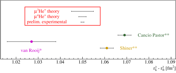
Figure 1: Difference of squared helion-to-alpha particle charge radii as obtained from laser spectroscopy of transitions in regular, electronic helium-3 and helium-4 atoms Shiner:1995:heliumSpec ; Rooij:2011:HeSpectroscopy ; CancioPastor:2012:PRL108 when combined with accurate theory (*Patkos:2017:HeIsoII , **Patkos:2016:HeIso ). A $4\,\sigma$ discrepancy persists. Also shown are the individual theory uncertainties which enter $r_{\mathrm{h}}^{2}-r_{\alpha}^{2}$ ($\mu^{4}$He⁺: Diepold:2016:muHe4theo , $\mu^{3}$He⁺: this work), as well as the expected uncertainty from our laser spectroscopy of the Lamb shift in muonic helium ions. Note that the combination of the two theoretical uncertainties should contain correlations which will partly cancel in the total uncertainty.

Several other experiments are on the way to contribute to the puzzle in the future Antognini:2016:PRP by precision spectroscopy measurements in electronic hydrogen Vutha:2012:H2S2P ; Beyer:2013:AdP_2S4P ; Peters:2013:AdP and He⁺ Herrmann:2009:He1S2S ; Kandula:2010:XUV_comb_metrology , as well as by electron scattering at very low $Q^{2}$ Mihovilovic:2013:ISR_exp_MAMI ; Gasparian:2014:PRad and muon-scattering Gilman:2013:MUSE . The He⁺ spectroscopy, in combination with our measurement in muonic helium ions, will be able to determine the Rydberg constant independently from hydrogen and deuterium. This is particularly interesting as the proton charge radius and the Rydberg constant are highly correlated which means that a change in the Rydberg constant could also resolve the puzzle Beyer:2013:AdP_2S4P .

The determination of the helion charge radius from muonic helium spectroscopy requires accurate knowledge of the corresponding theory. Similar to muonic hydrogen Antognini:2013:Annals , deuterium Krauth:2016:mud , and helium-4 ions Diepold:2016:muHe4theo , we feel therefore obliged to summarize the current knowledge on the state of theory contributions to the Lamb shift, fine-, and hyperfine structure in muonic helium-3 ions.

The accuracy to be expected from the experiment will be on the order of 20 GHz, which corresponds to $\sim 0.08\,\mathrm{meV}$ . In order to exploit the experimental precision, theory should, ideally, be accurate to a level of

$$\sigma_{\mathrm{theory}}\sim\mathcal{O}(0.01\,\mathrm{meV}).$$ (5)

This would result in a nearly hundred-fold better accuracy in the helion rms charge radius $r_{\mathrm{h}}$ compared to the value from electron scattering of

$$r_{\mathrm{h}}=1.973(14)\,\mathrm{fm},$$ (6)

deduced by Sick Sick:2014:HeZemach .

A more precise value has been given by Angeli et al. Angeli:2013:radii , which should be discarded. Their value is based on a charge radius extraction from $\mu^{4}$He⁺ by Carboni et al. Carboni:1978:LS_mu4he and on the isotope shift measurement from Shiner et al. Shiner:1995:heliumSpec . The Carboni measurement has however shown to be wrong Hauser:1992:LS_search , and the more recent measurement of the electronic isotope shift by van Rooij et al. Rooij:2011:HeSpectroscopy disagrees by $4\,\sigma$ from the Shiner one Shiner:1995:heliumSpec , see Fig. 1.

We anticipate here that the total uncertainty in the theoretical calculation of the Lamb shift transition amounts to 0.52 $\mathrm{meV}$ (corresponding to a relative uncertainty of $\sim$0.03%), neglecting the charge radius contribution to be extracted from the $\mu^{3}$He⁺ measurement. This value is completely dominated by the two-photon exchange contributions which are difficult to calculate but have seen wonderful progress in recent years NevoDinur:2016:TPE ; Hernandez:2016:POLupdate ; Carlson:2016:tpe . The total uncertainty of the pure QED contributions (without the two-photon exchange) amounts to 0.04 $\mathrm{meV}$ and is thus in the desired order of magnitude. Note that while the theory uncertainty from the two-photon exchange in $r_{\mathrm{p}}$ is of similar size as the experimental uncertainty (Eq. (1)), already for $\mu$d the theory uncertainty is vastly dominant (Eq. (3)). Experiments with muonic atoms are thus a sensitive tool to determine the two-photon exchange contributions.

2 Overview

The $n=2$ energy levels of the muonic helium-3 ion are sketched in Fig. 2. The helion has nuclear spin $I=1/2$, just as the proton. Hence the level scheme is very similar to the one of muonic hydrogen. However, the helion magnetic moment $g=-2.127\,625\,308(25)$ Mohr:2016:CODATA14 (here given in units of the nuclear magneton) is negative, which swaps the ordering of the hyperfine levels.

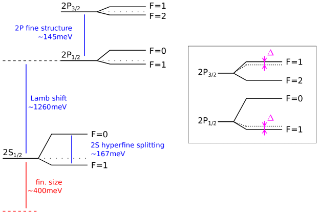
Figure 2: The 2S and 2P energy levels in the muonic helium-3 ion. The inset on the right displays the shift $\Delta$ of the 2P levels due to the mixing of levels with same quantum number $F$, as described in Sec. 5. The figure is not to scale.

A note on the sign convention of the Lamb shift contributions used in this article: The 2S level is shifted below the 2P levels due to the Lamb shift. This means that, fundamentally, the 2S Lamb shift should be given a negative sign.
However, following long-established conventions we assign the measured $2\textrm{S}_{1/2}\rightarrow 2\textrm{P}_{1/2}$ energy difference a positive sign, i.e. E(2P) – E(2S) $>$ 0. This is in accord with almost all publications we review here and we will mention explicitly when we have inverted the sign with respect to the original publications where the authors calculated level shifts.
Moreover, we obey the traditional definition of the Lamb shift as the terms beyond the Dirac equation and the leading order recoil corrections, i.e. excluding effects of the hyperfine structure. In particular, this means that the mixing of the hyperfine levels (Sec. 5) does not influence the Lamb shift.

The Lamb shift is dependent on the rms charge radius of the nucleus and is treated in Sec. 3. We split the Lamb shift contributions into nuclear structure-independent contributions and nuclear structure-dependent ones. The latter are composed out of one-photon exchange diagrams which represent the finite size effect and two-photon exchange diagrams which contain the polarizability contributions.

In Sec. 4, we treat the 2S hyperfine structure, which depends on the Zemach radius. It also has two-photon exchange contributions. However, these have not been calculated yet and can only be estimated with a large uncertainty.

In Sec. 5, we compile the 2P level structure which includes fine- and hyperfine splitting, and the mixing of the hyperfine levels Brodsky:1967:zeemanspectrum .

For the theory compilation presented here, we use the calculations from many sources mentioned in the following. The names of the authors of the respective groups are ordered alphabetically.

The first source is E. Borie who was one of the first to publish detailed calculations of many terms involved in the Lamb shift of muonic atoms. Her most recent calculations for $\mu$p, $\mu$d, $\mu^{4}$He⁺, and $\mu^{3}$He⁺ are all found in her Ref. Borie:2012:LS_revisited_AoP . Several updated versions of this paper are available on the arXiv. In this work we always refer to Borie:2014:arxiv_v7 which is version-7, the most recent one at the time of this writing.

The second source is the group of Elekina, Faustov, Krutov, and Martynenko et al. (termed “Martynenko group” in here for simplicity). The calculations we use in here are found in Krutov et al. Krutov:2014:JETP120_73 for the Lamb shift, in Martynenko et al. Martynenko:2010:2SHFS_muHe ; Martynenko:2008:muheHFS and Faustov et al. Faustov:2014:radrec for the 2S hyperfine structure, and Elekina et al. Elekina:2010:2Pmu3He for the 2P fine- and hyperfine structure.

Jentschura and Wundt calculated some Lamb shift contributions in their Refs. Jentschura:2011:SemiAnalytic ; Jentschura:2011:PRA84_012505 . They are referred to as “Jentschura” for simplicity.

The group of Ivanov, Karshenboim, Korzinin, and Shelyuto is referred to “Karshenboim group” for simplicity. Their calculations are found in Korzinin et al. Korzinin:2013:PRD88_125019 and in Karshenboim et al. Karshenboim:2012:PRA85_032509 for Lamb shift and fine structure contributions.

The group of Bacca, Barnea, Hernandez, Ji, and Nevo Dinur, situated at TRIUMF and Hebrew University, has performed ab initio calculations on two-photon exchange contributions of the Lamb shift. Their calculations are found in Nevo Dinur et al. NevoDinur:2016:TPE and Hernandez et al. Hernandez:2016:POLupdate . For simplicity we refer to them as “TRIUMF-Hebrew group”.

A recent calculation of the two-photon exchange using scattering data and dispersion relations has been performed by Carlson, Gorchtein, and Vanderhaeghen Carlson:2016:tpe .

Item numbers # in our tables follow the nomenclature in Refs. Antognini:2013:Annals ; Krauth:2016:mud . In the tables, we usually identify the “source” of all values entering “our choice” by the first letter of the (group of) authors given in adjacent columns (e.g. “B” for Borie). We denote as average “avg.” in the tables the center of the band covered by all values $v_{i}$ under consideration, with an uncertainty of half the spread, i.e.

$$\mathrm{avg.}~{}= \frac{1}{2}\,\big{[}{\rm MAX}(v_{i})+{\rm MIN}(v_{i})\big{]}$$ (7)

$$\pm \frac{1}{2}\,\big{[}{\rm MAX}(v_{i})-{\rm MIN}(v_{i})\big{]}.$$

If individual uncertainties are provided by the authors we add these in quadrature. We would like to point out that uncertainties due to uncalculated higher order terms are often not indicated explicitly by the authors. In the case some number is given, we include it in our sum. But in general our method can not account for uncertainty estimates of uncalculated higher order terms.

Throughout the paper, $Z$ denotes the nuclear charge with $Z=2$ for the helion and alpha particle, $\alpha$ is the fine structure constant, $m_{r}=199\,m_{e}$ is the reduced mass of the muon-nucleon system. “VP” is short for “vacuum polarization”, “SE” is “self-energy”, “RC” is “recoil correction”. “Perturbation theory” is abbreviated as “PT”, and SOPT and TOPT denote $2^{\rm nd}$ and $3^{\rm rd}$ order perturbation theory, respectively.

3 Lamb shift in muonic helium-3

3.1 Nuclear structure-independent contributions

Nuclear structure-independent contributions have been calculated by Borie, Martynenko group, Karshenboim group, and Jentschura. The contributions are listed in Tab. 1, labeled with #$i$. The leading contribution is the one-loop electron vacuum polarization (eVP) of order $\alpha(Z\alpha)^{2}$, the so-called Uehling term (see Fig. 3). It accounts for 99.5% of the radius-independent part of the Lamb shift, so it is very important that this contribution is well understood. There are two different approaches to calculate this term.

uehling (60,70) t3 b3 plain,tension=1.0t1,t3 plain,width=3 b1,b3 photont2,c1 photonc3,b2 smooth, pull=?, tension=0.3c0,c1,c2,c3 label=hb1 label.angle=-150,label=$\mu$t1 label.angle=180,label=$e$c2

Figure 3: Item #1, the leading order 1-loop electron vacuum polarization (eVP), also called Uehling term.

Borie Borie:2014:arxiv_v7 (p. 4, Tab.) and the Karshenboim group Korzinin:2013:PRD88_125019 (Tab. I) use relativistic Dirac wavefunctions to calculate a relativistic Uehling term (item #3). A relativistic recoil correction (item #19) has to be added to allow comparison to nonrelativistic calculations (see below). Borie provides the value of this correction explicitly in Borie:2014:arxiv_v7 Tab. 6, whereas the Karshenboim group only gives the total value which includes the correction, thus corresponding to ($\#3+\#19$).

Nonrelativistic calculations of the Uehling term (item #1) exist from the Martynenko group Krutov:2014:JETP120_73 (No. 1, Tab. 1) and Jentschura Jentschura:2011:PRA84_012505 , which are in very good agreement. Additionally, a relativistic correction (item #2) has to be applied. This relativistic correction already accounts for relativistic recoil effects (item #19). Item #2 has been calculated by the Martynenko group Krutov:2014:JETP120_73 (No. 7+10, Tab. 1), Borie Borie:2014:arxiv_v7 (Tab. 1), Jentschura Jentschura:2011:PRA84_012505 ; Jentschura:2011:SemiAnalytic (Eq. 17), and Karshenboim et al. Karshenboim:2012:PRA85_032509 , which agree well within all four groups, however do not have to be included in Borie’s and Korzinin et al.’s value because their relativistic Dirac wavefunction approach already accounts for relativistic recoil effects.

Both approaches agree well within the required uncertainty. As our choice for the Uehling term with relativistic correction ($\#1+\#2$) or ($\#3+\#19$) we take the average

$$\Delta E(\mathrm{Uehling\,+\,rel.~{}corr.})=1642.3962\pm 0.0018\,\mathrm{meV}.$$ (8)

Item #4, the second largest contribution in this section, is the two-loop eVP of order $\alpha^{2}(Z\alpha)^{2}$, the so-called Källén-Sabry term KallenSabry:1955 (see Fig. 4). It has been calculated by Borie Borie:2014:arxiv_v7 (p. 4, Tab.) and the Martynenko group Krutov:2014:JETP120_73 (No. 2, Tab. 1) which agree within 0.0037 $\mathrm{meV}$. As our choice we take the average.

Item #5 is the one-loop eVP in two Coulomb lines of order $\alpha^{2}(Z\alpha)^{2}$ (see Fig. 5). It has been calculated by Borie Borie:2014:arxiv_v7 (Tab. 6), the Martynenko group Krutov:2014:JETP120_73 (No. 9, Tab. 1), and Jentschura Jentschura:2011:SemiAnalytic (Eq. 13) of whom the latter two obtain the same result, which differs from Borie by 0.0033 $\mathrm{meV}$. As our choice we adopt the average.

The Karshenboim group Korzinin:2013:PRD88_125019 (Tab. I) has calculated the sum of item #4 and #5, the two-loop eVP (Källén-Sabry) and one-loop eVP in two Coulomb lines (Fig. 4 and 5). Good agreement between all groups is observed.

(a)

item_4 (60,70) t7 b7 plain,tension=1.0t1,t7 plain,width=3 b1,b7 phantom,tension=0.0001t4,c1,x1,c2,c4,x2,c5,b4 photon,tension=0t4,c1 photon,tension=0c2,c4 photon,tension=0c5,b4 plain,left,tension=0c1,c2,c1 plain,left,tension=0c4,c5,c4 label=hb1 label.angle=-150,label=$\mu$t1 phantomc1,l1,c2,l2 label.angle=180,label=$e$l1 phantomc4,l3,c5,l4 label.angle=180,label=$e$l3

(b)  

item_4b (60,70) t3 b3 plaint1,t2,t3 plain,width=3b1,b2,b3 photont2,c0 photonc4,b2 smooth,pull=?,tension=0.5c0,c1,c2,c3,c4,c5,c6,c7 photonc2,c6 label=hb1 label.angle=-150,label=$\mu$t1 label.angle=180,label=$e$c1

(c)  

item_4c (60,70) t3 b3 plaint1,t2,t3 plain,width=3b1,b2,b3 photont2,c0 photonc6,b2 smooth,pull=?,tension=0.8c0,c1,c2,c3,c4,c5,c6,c7,c8,c9,c10,c11 photonc7,c11 label=hb1 label.angle=-150,label=$\mu$t1 label.angle=180,label=$e$c1

Figure 4: Item #4, the two-loop eVP (Källen-Sabry) contribution. This is Fig. 1 (b,c,d) from the Martynenko group Krutov:2014:JETP120_73 .

 item_5 (100,70) t8 b8 plain,tension=1.0t1,t8 plain,width=3 b1,b8 phantom,tension=0.0001t3,c1,c2,b3 photon,tension=0t3,c1 photon,tension=0c2,b3 plain,left,tension=0c1,c2,c1 phantom,tension=0.0001t6,c3,c4,b6 photon,tension=0t6,c3 photon,tension=0c4,b6 plain,left,tension=0c3,c4,c3 label=hb1 label.angle=-150,label=$\mu$t1 phantomc1,l1,c2,l2 label.angle=110,label.dist=10,label=$e$l1 phantomc3,l3,c4,l4 label.angle=100,label.dist=10,label=$e$l3

Figure 5: Item #5, the one-loop eVP in 2-Coulomb lines.

Item #6+7 is the third order eVP of order $\alpha^{3}(Z\alpha)^{2}$. It has been calculated by the Martynenko group Krutov:2014:JETP120_73 (No. $4+11+12$, Tab. 1) and the Karshenboim group Korzinin:2013:PRD88_125019 (Tab. I). Borie Borie:2014:arxiv_v7 (p. 4) adopts the value from Karshenboim et al.. Martynenko et al. and Karshenboim et al. differ by $0.004\,\mathrm{meV}$, which is in agreement considering the uncertainty of $0.003\,\mathrm{meV}$ given by the Martynenko group. As our choice we adopt the average and obtain an uncertainty of 0.0036 $\mathrm{meV}$ via Gaussian propagation of uncertainty.

Item #29 is the second order eVP of order $\alpha^{2}(Z\alpha)^{4}$. It has been calculated by the Martynenko group Krutov:2014:JETP120_73 (No. $8+13$, Tab. 1) and the Karshenboim group Korzinin:2013:PRD88_125019 (Tab. VIII). Their values did agree in the case of $\mu$d, however for $\mu^{3}$He⁺ they differ by 0.004 $\mathrm{meV}$. This difference is twice as large as the value from Martynenko et al. but this contribution is small, so the uncertainty is not at all dominating. We reflect the difference by adopting the average as our choice.

Items #9, #10, and #9a are the terms of the Light-by-light (LbL) scattering contribution (see Fig. 6). The sum of the LbL terms is calculated by the Karshenboim group Korzinin:2013:PRD88_125019 (Tab. I). Borie Borie:2014:arxiv_v7 also lists the value from Karshenboim et al.. Item #9 is the Wichmann-Kroll term, or “1:3” LbL, which is of order $\alpha(Z\alpha)^{4}$. This item has also been calculated by Borie Borie:2014:arxiv_v7 (p. 4) and the Martynenko group Krutov:2014:JETP120_73 (No. 5, Tab. 1) who obtain the same result. Item #10 is the virtual Delbrück or “2:2” LbL, which is of order $\alpha^{2}(Z\alpha)^{3}$. Item #9a is the inverted Wichmann-Kroll term, or “3:1” LbL, which is of order $\alpha^{3}(Z\alpha)^{2}$. The sum of the latter two is also given by the Martynenko group Krutov:2014:JETP120_73 (No. 6, Tab. 1). As our choice we use the one from Karshenboim et al., who are the first and only group to calculate all three LbL contributions. The groups are in agreement when taking into account the uncertainty of 0.0006 $\mathrm{meV}$ given by Karshenboim et al..

(a)  

lblone (60,70) i1,v1,o1 i2,v2,v3,v4,o2 plaini1,v1,o1 plain,width=3i2,v2,v3,v4,o2

photonv1,c0 photonc2,v3

default, pull=?, tension=0.3c0,c1,c2,c3

photonc1,v2 photonc3,v4 label.angle=180,label=$e$c1 label=hi2 label.angle=-150,label=$\mu$i1

(b)  

lbltwo (60,70) i1,v1,v2,o1 i2,v3,v4,o2 plaini1,v1,v2,o1 plain,width=3i2,v3,v4,o2

photonv1,c0 photonv2,c3 photonv3,c1 photonv4,c2

default, pull=?, tension=0.5c0,c1,c2,c3

label.angle=120,label=$e$c1 label=hi2 label.angle=-150,label=$\mu$i1

(c)  

lblthree (60,70) i1,v1,v3,v4,o1 i2,v2,o2 plaini1,v1,v3,v4,o1 plain,width=3i2,v2,o2

photonv3,c0 photonc2,v2

default, pull=?, tension=0.3c0,c1,c2,c3

photonv1,c1 photonv4,c3 label.angle=180,label=$e$c1 label=hi2 label.angle=-150,label=$\mu$i1

Figure 6: The three contributions to Light-by-light scattering: (a) Wichmann-Kroll or “1:3” term, item #9, (b) Virtual Delbrück or “2:2” term, item #10, and (c) inverted Wichmann-Kroll or “3:1” term, item #9a^†.

Item #20 is the contribution from muon self-energy ($\mu$SE) and muon vacuum polarization ($\mu$VP) of order $\alpha(Z\alpha)^{4}$ (see Fig. 7). This item constitutes the third largest term in this section . This item has been calculated by Borie Borie:2014:arxiv_v7 (Tab. 2, Tab. 6) and the Martynenko group Krutov:2014:JETP120_73 (No. 24, Tab. 1). They differ by 0.001 $\mathrm{meV}$. As our choice we adopt the average.

(a)                            (b)

item_20 (70,60) t7 b7 plaint1,t7 plain,width=3b1,b7 photon,tension=0.1,left=1.0t3,t5 photont4,b4 label=hb1 label.angle=-150,label=$\mu$t1              (70,60) t7 b7 plaint1,t7 plain,width=3b1,b7 photont4,c1 photonc2,b4 smooth, pull=?, tension=0.3c1,l1,c2,l2 label.angle=180,label=$\mu$l1 label=hb1 label.angle=-150,label=$\mu$t1

Figure 7: Item #20, the muon-self energy (a) and the muon vacuum polarization (b), $\alpha(Z\alpha)^{4}$.

Items #11, #12, #30, #13, and #31 are all corrections to VP or $\mu$SE and of order $\alpha^{2}(Z\alpha)^{4}$.

Item #11 is the $\mu$SE correction to eVP (see Fig. 8). It has been calculated by all four groups. Martynenko et al. calculate this term (Eq. 99) in Krutov:2014:JETP120_73 , however in their table (No. 28) they use the more exact calculation from Jentschura. Jentschura Jentschura:2011:SemiAnalytic (Eq. 29), and the Karshenboim group Korzinin:2013:PRD88_125019 (Tab. VIII a) are in excellent agreement. Borie Borie:2014:arxiv_v7 (Tab. 16) differs significantly because she only calculates a part of this contribution in her App. C. This value does not enter her sum and thus is also not considered in here. On p. 12 of Borie:2014:arxiv_v7 she states that this value should be considered as an uncertainty. As our choice we adopt the number from Jentschura and Karshenboim et al..

(a)  

item_11a (60,70) t7 b7 plain,tension=1.0t1,t7 plain,width=3 b1,b7 photon,tension=0.1,left=1.0t3,t5 phantom,tension=0.0001t4,c1,c2,b4 photon,tension=0t4,c1 photon,tension=0c2,b4 plain,left,tension=0c1,c2,c1 phantomc1,l1,c2,l2 label.angle=180,label=$e$l1 label=hb1 label.angle=-150,label=$\mu$t1

(b)  

item_11b (60,70) t7 b7 plain,tension=1.0t1,t7 plain,width=3 b1,b7 photon,tension=0.1,left=1.0t2,t4 phantom,tension=0.0001t5,c1,c2,b5 photon,tension=0t5,c1 photon,tension=0c2,b5 plain,left,tension=0c1,c2,c1 phantomc1,l1,c2,l2 label.angle=180,label=$e$l1 label=hb1 label.angle=-150,label=$\mu$t1

(c)  

item_11c (60,70) t7 b7 plain,tension=1.0t1,t7 plain,width=3 b1,b7 photon,tension=0.1,left=1.0t4,t6 phantom,tension=0.0001t3,c1,c2,b3 photon,tension=0t3,c1 photon,tension=0c2,b3 plain,left,tension=0c1,c2,c1 phantomc1,l1,c2,l2 label.angle=180,label=$e$l1 label=hb1 label.angle=-150,label=$\mu$t1

Figure 8: Item #11, muon self-energy corrections to the electron vacuum polarization $\alpha^{2}(Z\alpha)^{4}$. This figure is Fig. 2 from Jentschura Jentschura:2011:AnnPhys1 . It corresponds to Fig. 6(a) from Karshenboim Korzinin:2013:PRD88_125019 .

Item #12 is the eVP in $\mu$SE (see Fig. 9). This item has been calculated by the Martynenko group Krutov:2014:JETP120_73 (No. 27, Tab. 1) and the Karshenboim group Korzinin:2013:PRD88_125019 (Tab. VIII d), which are in perfect agreement. On p. 10 of Borie:2014:arxiv_v7 Borie mentions that she included the “fourth order electron loops” in “muon Lamb shift, higher order” term, which is our item #21. As we include item #21 from Borie, we will not on top include item #12.

 Mart_fig11b (70,80) i9 o9 plain,tension=1.0i5,t1,t2,t3,o5 plain,width=3i1,b2,o1 photon,tension=0t2,b2 phantomi7,c1 phantomo7,c2 photon,tension=0,left=0.3t1,c1 photon,tension=0,left=0.3c2,t3 plain,left,tension=0.5c1,c2,c1 label.angle=100,label.dist=10,label=$e$c1 label=hi1 label.angle=-150,label=$\mu$i5

Figure 9: Item #12, eVP loop in SE are radiative corrections with VP effects. This is Fig. 11(b) from a publication by the Martynenko group Krutov:2014:JETP120_73 which is the same as Fig. 4 in Pachucki Pachucki:1996:LSmup . It is Karshenboim’s Fig. 6(d) in Ref. Korzinin:2013:PRD88_125019 .

Item #30 is the hadronic vacuum polarization (hVP) in $\mu$SE (see Fig. 10). This item has only been calculated by the Karshenboim group Korzinin:2013:PRD88_125019 (Tab. VIII e) which we adopt as our choice.

 item_30 (70,80) i9 o9 plain,tension=1.0i5,t1,t2,t3,o5 plain,width=3i1,b2,o1 photon,tension=0t2,b2 phantomi7,c1 phantomo7,c2 photon,tension=0,left=0.3t1,c1 photon,tension=0,left=0.3c2,t3 dashes,left,tension=0.5c1,c2,c1 label.angle=100,label.dist=10,label=$h$c1 label=hi1 label.angle=-150,label=$\mu$i5

Figure 10: Item #30, hadronic VP in SE contribution, corresponds to Fig. 6(e) in Karshenboim et al.’s Korzinin:2013:PRD88_125019 .

Item #13 is the mixed $e$VP + $\mu$VP (see Fig. 11). The calculations from Borie Borie:2014:arxiv_v7 (p. 4) and the Martynenko group Krutov:2014:JETP120_73 (No. 3, Tab. 1) roughly agree, whereas the value from the Karshenboim group Korzinin:2013:PRD88_125019 (Tab. VIII b) is 0.002 $\mathrm{meV}$ larger. As our choice we take the average.

(a)  

item_13a (60,70) t7 b7 plain,tension=1.0t1,t7 plain,width=3 b1,b7 phantom,tension=0.0001t4,c1,x1,c2,c4,x2,c5,b4 photon,tension=0t4,c1 photon,tension=0c2,c4 photon,tension=0c5,b4 plain,left,tension=0c1,c2,c1 plain,left,tension=0c4,c5,c4 label=hb1 label.angle=-150,label=$\mu$t1 phantomc1,l1,c2,l2 label.angle=180,label=$e$l1 phantomc4,l3,c5,l4 label.angle=180,label=$\mu$l3

(b)  

item_13b (100,70) t8 b8 plain,tension=1.0t1,t8 plain,width=3 b1,b8 phantom,tension=0.0001t3,c1,c2,b3 photon,tension=0t3,c1 photon,tension=0c2,b3 plain,left,tension=0c1,c2,c1 phantom,tension=0.0001t6,c3,c4,b6 photon,tension=0t6,c3 photon,tension=0c4,b6 plain,left,tension=0c3,c4,c3 label=hb1 label.angle=-150,label=$\mu$t1 phantomc1,l1,c2,l2 label.angle=110,label.dist=10,label=$e$l1 phantomc3,l3,c4,l4 label.angle=100,label.dist=10,label=$\mu$l3

Figure 11: Item #13, the mixed eVP-$\mu$VP contribution.

Item #31 is the mixed $e$VP + hVP (see Fig. 12) which has only been calculated by the Karshenboim group Korzinin:2013:PRD88_125019 (Tab. VIII c). We adopt their value as our choice.

(a)  

item_31a (60,70) t7 b7 plain,tension=1.0t1,t7 plain,width=3 b1,b7 phantom,tension=0.0001t4,c1,x1,c2,c4,x2,c5,b4 photon,tension=0t4,c1 photon,tension=0c2,c4 photon,tension=0c5,b4 plain,left,tension=0c1,c2,c1 dashes,left,tension=0c4,c5,c4 label=hb1 label.angle=-150,label=$\mu$t1 phantomc1,l1,c2,l2 label.angle=180,label=$e$l1 phantomc4,l3,c5,l4 label.angle=180,label=$h$l3

(b)  

item_31b (100,70) t8 b8 plain,tension=1.0t1,t8 plain,width=3 b1,b8 phantom,tension=0.0001t3,c1,c2,b3 photon,tension=0t3,c1 photon,tension=0c2,b3 plain,left,tension=0c1,c2,c1 phantom,tension=0.0001t6,c3,c4,b6 photon,tension=0t6,c3 photon,tension=0c4,b6 dashes,left,tension=0c3,c4,c3 label=hb1 label.angle=-150,label=$\mu$t1 phantomc1,l1,c2,l2 label.angle=110,label.dist=10,label=$e$l1 phantomc3,l3,c4,l4 label.angle=100,label.dist=10,label=$h$l3

Figure 12: Item #31, the mixed eVP- and hadronic VP contribution, comes from the Uehling correction to the hadronic VP correction. See Fig. 6(c) in Karshenboim et al.’s Korzinin:2013:PRD88_125019 .

Item #32, the muon VP in SE correction shown in Fig. 13 is not included as a separate item in our Tab. 1. It should already be automatically included in the QED contribution which has been rescaled from the QED of electronic ³He⁺ by a simple mass replacement $m_{e}\rightarrow m_{\mu}$ Karshenboim:PC:2015 . This is the case only for QED contributions where the particle in the loop is the same as the bound particle - like in this case, a muon VP correction in a muonic atom. The size of this item #32 can be estimated from the relationship found by Borie Borie:1981:HVP , that the ratio of hadronic to muonic VP is 0.66. With the Karshenboim group’s value of item #30 Korzinin:2013:PRD88_125019 one would obtain a value for item #32 of $-0.0004/0.66\,\mathrm{meV}=-0.0006\,\mathrm{meV}$. This contribution is contained in our item #21, together with the dominating item #12 (see also p. 10 of Ref. Borie:2014:arxiv_v7 ).

item_32 (70,70) i9 o9 plain,tension=1.0i5,t1,t2,t3,o5 plain,width=3i1,b2,o1 photon,tension=0t2,b2 phantomi7,c1 phantomo7,c2 photon,tension=0,left=0.3t1,c1 photon,tension=0,left=0.3c2,t3 plain,left,tension=0.5c1,c2,c1 label.angle=100,label.dist=10,label=$\mu$c1 label=hi1 label.angle=-150,label=$\mu$i5

Figure 13: Item #32, muon VP in SE contribution, is automatically included in a rescaled electronic ³He⁺ QED value of higher order SE contributions (see text).

Item #21 is a higher-order correction to $\mu$SE and $\mu$VP of order $\alpha^{2}(Z\alpha)^{4}$ and $\alpha^{2}(Z\alpha)^{6}$. This item has only been calculated by Borie Borie:2014:arxiv_v7 (Tab. 2, Tab. 6). On p. 10 she points out that this contribution includes the “fourth order electron loops”, which is our item #12. It also contains our item #32. We adopt her value as our choice.

Item #14 is the hadronic VP of order $\alpha(Z\alpha)^{4}$. It has been calculated by Borie Borie:2014:arxiv_v7 (Tab. 6) and the Martynenko group Krutov:2014:JETP120_73 (No. 29, Tab. 1). Borie assigns a 5% uncertainty to their value. However, in her Ref. Borie:2014:arxiv_v7 there are two different values of item #14, the first on p. 5 (0.219 $\mathrm{meV}$) and the second in Tab. 6 on p. 16 (0.221 $\mathrm{meV}$). Regarding the given uncertainty this difference is not of interest. In our Tab. 1, we report the larger value which is further from that of the Martynenko group in order to conservatively reflect the scatter. Martynenko et al. did not assign an uncertainty to their value. However, for $\mu$d Krutov:2011:PRA84_052514 they estimated an uncertainty of 5%. As our choice we take the average of their values and adopt the uncertainty of 5% (0.011 $\mathrm{meV}$).

Item #17 is the Barker-Glover correction Barker:1955 . It is a recoil correction of order $(Z\alpha)^{4}m_{r}^{3}/M^{2}$ and includes the nuclear Darwin-Foldy term that arises due to the Zitterbewegung of the nucleus. As already discussed in App. A of Krauth:2016:mud , we follow the atomic physics convention Jentschura:2011:DF , which is also adopted by CODATA in their report from 2010 Mohr:2012:CODATA10 and 2014 Mohr:2016:CODATA14 . This convention implies that item #17 is considered as a recoil correction to the energy levels and not as a part of the rms charge radius. This term has been calculated by Borie Borie:2014:arxiv_v7 (Tab. 6), the Martynenko group Krutov:2014:JETP120_73 (No. 21, Tab. 1), and Jentschura Jentschura:2011:PRA84_012505 and Jentschura:2011:SemiAnalytic (Eq. A.3). As our choice we use the number given by Borie and Jentschura as they give one more digit.

Item #18 is the term called “recoil, finite size” by Borie. It is of order $(Z\alpha)^{5}\langle r\rangle_{(2)}/M$ and is linear in the first Zemach moment. It has first been calculated by Friar Friar:1978:Annals (see Eq. F5 in App. F) for hydrogen and has later been given by Borie Borie:2014:arxiv_v7 for $\mu$d, $\mu^{4}$He⁺, and $\mu^{3}$He⁺. We discard item #18 because it is considered to be included in the elastic TPE Pachucki:PC:2015 ; Yerokhin:2016:RCFS . It has also been discarded in $\mu$p Antognini:2013:Annals , $\mu$d Krauth:2016:mud , and $\mu^{4}$He⁺ Diepold:2016:muHe4theo . For the muonic helium-3 ion, item #18 in Borie:2014:arxiv_v7 (Tab. 6) amounts to 0.4040 $\mathrm{meV}$, which is five times larger than the experimental uncertainty of about 0.08 $\mathrm{meV}$ (see Eq. 5), so it is important that the treatment of this contribution is well understood.

Item #22 and #23 are relativistic recoil corrections of order $(Z\alpha)^{5}$ and $(Z\alpha)^{6}$, respectively. Item #22 has been calculated by Borie Borie:2014:arxiv_v7 (Tab. 6), the Martynenko group Krutov:2014:JETP120_73 (No. 22, Tab. 1), and Jentschura Jentschura:2011:SemiAnalytic (Eq. 32). They agree perfectly. Item #23 has only been calculated by the Martynenko group Krutov:2014:JETP120_73 (No. 23, Tab. 1) whose value we adopt as our choice.

Item #24 are higher order radiative recoil corrections of order $\alpha(Z\alpha)^{5}$ and $(Z^{2}\alpha)(Z\alpha)^{4}$. This item has been calculated by Borie Borie:2014:arxiv_v7 (Tab. 6) and the Martynenko group Krutov:2014:JETP120_73 (No. 25, Tab. 1). Their values differ by 0.015 $\mathrm{meV}$. As our choice we adopt the average.

Item #28 is the radiative (only eVP) recoil of order $\alpha(Z\alpha)^{5}$. It consists of three terms which have been calculated by Jentschura and Wundt Jentschura:2011:SemiAnalytic (Eq. 46). We adopt their value as our choice. Note that a second value (0.0072 $\mathrm{meV}$) is found in Jentschura:2011:PRA84_012505 . However, this value is just one of the three terms, namely the seagull term, and is already included in #28 (see Jentschura:2011:SemiAnalytic , Eq. 46).

The total sum of the QED contributions without explicit nuclear structure dependence is summarized in Tab. 1 and amounts to

$$\Delta E_{\mathrm{r\mathrm{-indep.}}}^{\mathrm{LS}}=1644.3466\pm 0.0146\,\mathrm{meV}.$$ (9)

Note that Borie, on p. 15 in Ref. Borie:2014:arxiv_v7 attributes an uncertainty of 0.6 $\mathrm{meV}$ to her total sum. The origin of this number remains unclear Borie:PC:2017 . Its order of magnitude is neither congruent with the other uncertainties given in Ref. Borie:2014:arxiv_v7 nor with other uncertainties collected in our summary. Thus it will not be taken into account.

3.2 Nuclear structure contributions

Terms that depend on the nuclear structure are separated into one-photon exchange (OPE) contributions and two-photon exchange (TPE) contributions.

The OPE terms (also called radius-dependent contributions) represent the finite size effect which is by far the largest part of the nuclear structure contributions and are discussed in Sec. 3.2.1. They are parameterizable with a coefficient times the rms charge radius squared. These contributions are QED interactions with nuclear form factor insertions.

The TPE terms can be written as a sum of elastic and inelastic terms, where the latter describe the polarizability of the nucleus. These involve contributions from strong interaction and therefore are much more complicated to evaluate, which explains why the dominant uncertainty originates from the TPE part. The TPE contributions are discussed in more detail in Sec. 3.2.2.

The main nuclear structure corrections to the $n$S states have been given up to order $(Z\alpha)^{6}$ by Friar Friar:1978:Annals (see Eq. (43a) therein)

$$\Delta E_{\rm fin.size}=\frac{2\pi Z\alpha}{3}|\Psi(0)|^{2}\left(\langle r^{2}\rangle-\frac{Z\alpha m_{r}}{2}\langle r^{3}\rangle_{(2)}+(Z\alpha)^{2}(F_{\rm REL}+m_{r}^{2}F_{\rm NREL})\right),$$ (10)

where $\Psi(0)$ is the muon wave function at the origin, $\langle r^{2}\rangle$ is the second moment of the charge distribution of the nucleus, i.e. the square of the rms charge radius, $r_{E}^{2}$. $\langle r^{3}\rangle_{(2)}$ is the Friar moment , and $F_{\rm REL}$ and $F_{\rm NREL}$ contain various moments of the nuclear charge distribution (see Eq. (43b) and (43c) in Ref. Friar:1978:Annals ). Analytic expressions for some simple model charge distributions are listed in App. E of Ref. Friar:1978:Annals .

As the Schrödinger wavefunction at the origin $\Psi(0)$ is nonzero only for S states, it is in leading order only the S states which are affected by the finite size. However, using the Dirac wavefunction a nonzero contribution appears for the $2\textrm{P}_{1/2}$ level Ivanov:2001:LS . This contribution affects the values for the Lamb shift and the fine structure and is taken into account in the section below.

The Friar moment $\langle r^{3}\rangle_{(2)}$ has not been included in $\mu$d Krauth:2016:mud because of a cancellation Friar:1997:PRA56_5173 ; Pachucki:2011:PRL106_193007 ; Friar:2013:PRC88_034004 with a part of the inelastic nuclear polarizability contributions. The TRIUMF-Hebrew group pointed out NevoDinur:2016:TPE ; Hernandez:2016:POLupdate , that in the case of $\mu^{3}$He⁺ however, a smaller uncertainty might be achieved treating each term separately. This discussion is not finished yet and we will therefore continue with the more conservative treatment as before. See Sec. 3.2.2.

Table 1: All known nuclear structure-independent contributions to the Lamb shift in $\mu^{3}$He⁺. Values are in meV. Item numbers “#” in the 1st column follow the nomenclature of Refs. Antognini:2013:Annals ; Krauth:2016:mud , which in turn follow the supplement of Ref. Pohl:2010:Nature_mup1 . Items “#“ with a dagger ^† were labeled “New” in Ref. Antognini:2013:Annals , but we introduced numbers in Ref. Krauth:2016:mud for definiteness. For Borie Borie:2014:arxiv_v7 we refer to the most recent arXiv version-7 which contains several corrections to the published paper Borie:2012:LS_revisited_AoP (available online 6 Dec. 2011). For the Martynenko group, numbers #1 to #29 refer to rows in Tab. I of Ref. Krutov:2014:JETP120_73 . Numbers in parentheses refer to equations in the respective paper.

#	Contribution	Borie (B)		Martynenko group (M)		Jentschura (J)		Karshenboim group (K)		Our choice
		Borie:2014:arxiv_v7		Krutov et al. Krutov:2014:JETP120_73		Jentschura, Wundt Jentschura:2011:SemiAnalytic		Karshenboim et al. Karshenboim:2012:PRA85_032509		value		source	Fig.
						Jentschura Jentschura:2011:PRA84_012505		Korzinin et al. Korzinin:2013:PRD88_125019
1	NR one-loop electron VP (eVP)			$1641.8862$	#1	$1641.885$	Jentschura:2011:PRA84_012505
2	Rel. corr. (Breit-Pauli)	$(0.50934)~{}$	Tab. 1	$0.5093$	#7+#10	$0.509344$	Jentschura:2011:SemiAnalytic (17), Jentschura:2011:PRA84_012505	$(0.509340)$	Karshenboim:2012:PRA85_032509 Tab. IV
3	Rel. one-loop eVP	$1642.412$	Tab. p. 4
19	Rel. RC to eVP, $\alpha(Z\alpha)^{4}$	$-0.0140$	Tab. 1+6
	Sum of the above	$1642.3980$	3+19	$1642.3955$	1+2	$1642.3943$	1+2	$1642.3954$	Korzinin:2013:PRD88_125019 Tab. I	$1642.3962$	$~{}\pm~{}0.0018$	avg	3
4	Two-loop eVP (Käll$\acute{\mathrm{e}}$n-Sabry)	$11.4107$	Tab. p. 4	$11.4070$	#2					$11.4089$	$\pm~{}0.0019$	avg.	4
5	One-loop eVP in 2-Coulomb lines $\alpha^{2}(Z\alpha)^{2}$	$1.674$	Tab. 6	$1.6773$	#9	$1.677290$	Jentschura:2011:SemiAnalytic (13)			$1.6757$	$~{}\pm~{}0.0017$	avg.	5
	Sum of 4 and 5	$13.0847$	4+5	$13.0843$	4+5			$13.0843$	Korzinin:2013:PRD88_125019 Tab. I	$(13.0846)$
6+7	Third order VP	$0.073(3)$	p. 4	$0.0689$	#4+#12+#11			$0.073(3)$	Korzinin:2013:PRD88_125019 Tab. I	$0.0710$	$\pm~{}0.0036$	avg.
29	Second-order eVP contribution $\alpha^{2}(Z\alpha)^{4}m$			$0.0018$	#8+#13			$0.00558$	Korzinin:2013:PRD88_125019 Tab. VIII “eVP2”	$0.0037$	$~{}\pm~{}0.0019$	avg
9	Light-by-light “1:3”: Wichmann-Kroll	$-0.01969$	p. 4	$-0.0197$	#5								6a
10	Virtual Delbrück, “2:2” LbL			$\left.\rule{0.0pt}{12.91663pt}\right\}0.0064$	#6								6b
9a†	“3:1” LbL												6c
	Sum: Total light-by-light scatt.	$-0.0134(6)$	p.5+Tab.6	$-0.0133$	9+10+9a			$-0.0134(6)$	Korzinin:2013:PRD88_125019 Tab. I	$-0.0134$	$\pm~{}0.0006$	K
20	$\mu$SE and $\mu$VP	$-10.827368$	Tab. 2+6	$-10.8286$	#24					$-10.8280$	$\pm~{}0.0006$	avg.	7
11	Muon SE corr. to eVP $\alpha^{2}(Z\alpha)^{4}$	$(-0.1277)~{}$	Tab. 16	$-0.0627$	#28	$-0.06269$	Jentschura:2011:SemiAnalytic (29)	$-0.06269$	Korzinin:2013:PRD88_125019 Tab. VIII (a)	$-0.06269$		J, K	8
12	eVP loop in self-energy $\alpha^{2}(Z\alpha)^{4}$	incl. in 21		$-0.0299$	#27			$-0.02992$	Korzinin:2013:PRD88_125019 Tab. VIII (d)	incl. in 21		B	9
30	Hadronic VP loop in self-energy $\alpha^{2}(Z\alpha)^{4}m$							$-0.00040(4)$	Korzinin:2013:PRD88_125019 Tab. VIII (e)	$-0.00040$	$\pm~{}0.00004$	K	10
13	Mixed eVP + $\mu$VP	$0.00200$	p. 4	$0.0022$	#3			$0.00383$	Korzinin:2013:PRD88_125019 Tab. VIII (b)	$0.0029$	$\pm~{}0.0009$	avg	11
31	Mixed eVP + hadronic VP							$0.0024(2)$	Korzinin:2013:PRD88_125019 Tab. VIII (c)	$0.0024$	$\pm~{}0.0002$	K	12
21	Higher-order corr. to $\mu$SE and $\mu$VP	$-0.033749$	Tab. 2+6							$-0.033749$		B
	Sum of 12, 30, 13, 31, and 21	$-0.031749$	13+21	$-0.0277$	12+13			$-0.0241(2)$	12+30+13+31	$-0.0288$		sum
14	Hadronic VP	$0.221(11)$	Tab. 6	$0.2170$	#29					$0.219$	$\pm~{}0.011$	avg.
17	Recoil corr. $(Z\alpha)^{4}m_{r}^{3}/M^{2}$ (Barker-Glover)	$0.12654$	Tab. 6	$0.1265$	#21	$0.12654$	Jentschura:2011:SemiAnalytic (A.3) Jentschura:2011:PRA84_012505 (15)			$0.12654$		B, J
18	Recoil, finite size	$(0.4040(10))~{}$
22	Rel. RC $(Z\alpha)^{5}$	$-0.55811$	p.9+Tab.6	$-0.5581$	#22	$-0.558107$	Jentschura:2011:SemiAnalytic (32)			$-0.558107$		J
23	Rel. RC $(Z\alpha)^{6}$			$0.0051$	#23					$0.0051$		M
24	Higher order radiative recoil corr.	$-0.08102$	p.9+Tab.6	$-0.0656$	#25					$-0.0733$	$\pm~{}0.0077$	avg.
28†	Rad. (only eVP) RC $\alpha(Z\alpha)^{5}$					$0.004941$				$0.004941$		J
	Sum	1644.3916		$1644.3431$						${\bf 1644}\bf.{\bf 3466}$	$\pm~{}{\bf 0}\bf.{\bf 0146}$

3.2.1 One-photon exchange contributions (finite size effect)

Finite size contributions have been calculated by Borie (Borie:2014:arxiv_v7 Tab. 14), the Martynenko group (Krutov:2014:JETP120_73 Tab. 1), and the Karshenboim group (Karshenboim:2012:PRA85_032509 Tab. III). All of these contributions are listed in Tab. 2, labeled with #r$i$.

Most of the terms, given in Tab. 2, can be parameterized as $c\cdot{r_{E}}^{2}$ with coefficients $c$ in units of meV  $\mathrm{fm}^{-2}$. Borie and Karshenboim et al. have provided the contributions in this parameterization, whereas Martynenko et al. provide the total value in units of energy. However, the value of their coefficients can be obtained by dividing their numbers by ${r_{E}}^{2}$ . The value they used for the charge radius $r_{E}$ is 1.9660 fm  Martynenko:PC:2016 . In this way the numbers from Martynenko et al. can be compared with the ones from the other groups.

Item #r1, the leading term of Eq. (10), is the one-photon exchange with a helion form factor (FF) insertion (see Fig. 14). Item #r1 is of order $(Z\alpha)^{4}m_{r}^{3}$ and accounts for 99% of the OPE contributions. Borie (Borie:2014:arxiv_v7 Tab. 14, $b_{a}$), the Martynenko group (Krutov:2014:JETP120_73 No. 14), and the Karshenboim group (Karshenboim:2012:PRA85_032509 Tab. III, $\Delta_{FNS}^{(0)}$) obtain the same result which we adopt as our choice. This contribution is much larger than the following terms, but its absolute precision is worse, which we indicate by introducing an uncertainty. For that we take the value from Borie which is given with one more digit than the values of the other authors and attribute an uncertainty of 0.0005 $\mathrm{meV}$, which may arise from rounding.

ope (70,70) i1,o1 i2,o2 plain,tension=1.0i1,v1,o1 plain,width=3i2,v2,o2 photon,tension=0v1,v2 decor.shape=circle,decor.filled=full,decor.size=10v2 label=hi2 label.angle=-150,label=$\mu$i1

Figure 14: Item #r1, the leading nuclear finite size correction stems from a one-photon interaction with a helion form factor insertion, indicated by the thick dot.

Item #r2 and #r2’ are the radiative correction of order $\alpha(Z\alpha)^{5}$. The equation used for the calculation of item #r2 is given in Eq. (10) of Eides:1997:two-photon . It has been calculated by Borie Borie:2014:arxiv_v7 (Tab. 14, $b_{b}$) and the Martynenko group Krutov:2014:JETP120_73 (No. 26, only Eq. (92)). Note that the value from the Martynenko group was published with a wrong sign.
Very recently the Martynenko group updated their calculation of higher-order finite size corrections Faustov:2017:rad_fin_size using more realistic, measured nuclear form factors. The results contain a coefficient (in our work termed item #r2) which agrees with the old value, and an additional, previously unkown term which cannot be parametrized with $r_{\mathrm{h}}^{2}$ and therefore is given as a constant. This constant is found in our Tab. 2 as item #r2’. In Ref. Faustov:2017:rad_fin_size the values are given for the 1S state but can easily be transferred to the 2S state via the $1/n^{3}$ scaling. For the 2S state this results in

$$\begin{split}1/8\times(&-0.6109)\,\mathrm{meV}\\ =&~{}1/8\times(-0.1946\,r_{\mathrm{h}}^{2}+0.1412)\,\mathrm{meV}\\ =&~{}-0.0243\,\mathrm{meV}/\,\mathrm{fm}^{2}r_{\mathrm{h}}^{2}+0.0177\,\mathrm{meV}.\end{split}$$ (11)

Borie and Martynenko get the same result for item #r2, which we adopt as our choice. Additionally we adopt the constant term from Martynenko as item #r2’.

Item #r3 and #r3’ are the finite size corrections of order $(Z\alpha)^{6}$. They have first been calculated in Ref. Friar:1978:Annals . Item #r3 and #r3’ consider third-order perturbation theory in the finite size potential correction and relativistic corrections of the Schrödinger wave functions. There are also corrections in the TPE of the same order $(Z\alpha)^{6}$, but these are of different origin. Borie Borie:2014:arxiv_v7 (Tab. 14, $b_{c}$ and Tab. 6) and the Martynenko group Krutov:2014:JETP120_73 (Eq. (91)) follow the procedure in Ref. Friar:1978:Annals and then separate their terms into a part with an explicit ${r_{E}}^{2}$ dependence (item #r3) and another one which is usually evaluated with an exponential charge distribution, since a model independent calculation of this term is prohibitively difficult Borie:2014:arxiv_v7 . Differences in sorting the single terms have already been noticed in the $\mu$d case Krauth:2016:mud , where we mentioned that e.g. the term $\langle r^{2}\rangle\langle\ln(\mu r)\rangle$ in $F_{\rm REL}$ of Eq. 10 is attributed to #r3 and #r3’ by Martynenko et al. and Borie, respectively. The difference in this case amounts to 0.007 $\mathrm{meV}$ for #r3’. Note that in Eq. (91) from the Martynenko group Krutov:2014:JETP120_73 , the charge radius has to be inserted in units of GeV^-1, with $r_{E}=1.966\,\mathrm{fm}\,\widehat{=}\,9.963\,\mathrm{GeV}^{-1}$.

Item #r4 is the one-loop $e$VP correction (Uehling) of order $\alpha(Z\alpha)^{4}$. It has been calculated by all three groups, Borie Borie:2014:arxiv_v7 (Tab. 14, $b_{d}$), Martynenko et al. Krutov:2014:JETP120_73 (No. 16, Eq. (69)), and Karshenboim et al. Karshenboim:2012:PRA85_032509 (Tab. III, $\Delta E_{FNS}^{(2)}$). On p. 31 of Borie:2014:arxiv_v7 , Borie notes that she included the correction arising from the Källén-Sabry potential in her $b_{d}$. This means that her value already contains item #r6, which is the two-loop $e$VP correction of order $\alpha^{2}(Z\alpha)^{4}$. Item #r6 has been given explicitly only by the Martynenko group Krutov:2014:JETP120_73 (No. 18, Eq. 73). The sum of Martynenko et al.’s #r4 and #r6 differs by 0.016 $\mathrm{meV}$/fm² from Borie’s result. Using a charge radius of 1.9660 fm this corresponds to roughly 0.06 $\mathrm{meV}$ and, hence, causes the largest uncertainty in the radius-dependent OPE part. The origin of this difference is not clear Borie:PC:2017 ; Martynenko:PC:2017 . A clarification of this difference is desired but does not limit the extraction of the charge radius. As our choice we take the average of the sum (#r4+#r6) of these two groups. The resulting average does also reflect the value for #r4 provided by Karshenboim et al. Karshenboim:2012:PRA85_032509 .

Item #r5 is the one-loop $e$VP correction (Uehling) in second order perturbation theory (SOPT) of order $\alpha(Z\alpha)^{4}$. It has been calculated by all three groups, Borie Borie:2014:arxiv_v7 (Tab. 14, $b_{e}$), the Martynenko group Krutov:2014:JETP120_73 (No. 17, Eq. 70), and the Karshenboim group Karshenboim:2012:PRA85_032509 (Tab. III, $\Delta E_{FNS}^{(1)}$). On p. 31 of Borie:2014:arxiv_v7 , Borie notes that she included the two-loop corrections to $\epsilon_{VP2}$ in her $b_{e}$. This means that her value already contains item #r7, which is the two-loop $e$VP in SOPT of order $\alpha^{2}(Z\alpha)^{4}$. Item #r7 has only been given explicitly by the Martynenko group Krutov:2014:JETP120_73 (No. 19). The sum of Martynenko et al.’s #r5+#r7 differs by 0.003 $\mathrm{meV}$ from Borie’s result. As our choice we take the average of the sum (#r5+#r7) of these two groups. Again here, our choice reflects the value for #r5 provided by Karshenboim et al. Karshenboim:2012:PRA85_032509 , too.

Item #r8 is the finite size correction to the $2\textrm{P}_{1/2}$ level of order $(Z\alpha)^{6}$. It has only been calculated by Borie Borie:2014:arxiv_v7 (Tab. 14, $b(2p_{1/2}$). This correction is the smallest in this section and is the only term which affects the $2\textrm{P}_{1/2}$ level. In consequence, the effect on the Lamb shift is inverse, i.e. if the 2P level is lifted “upwards”, the Lamb shift gets larger. Thus, in contrast to Borie, we include this correction with a positive sign. At the same time this term decreases the fine structure ($2\textrm{P}_{3/2}-2\textrm{P}_{1/2}$ energy difference) and is hence listed in Tab. 4 as item #f10 with a negative sign.

The total sum of the QED contributions with an explicit dependence of ${r_{E}}^{2}$ is summarized in Tab. 2 and amounts to

$$\Delta E_{\mathrm{r\mathrm{-dep.}}}^{\mathrm{LS}}({r_{E}}^{2})\\ =-103.5184(98)\,\mathrm{meV}\,\mathrm{fm}^{-2}\,{r_{E}}^{2}+0.1354(33)\,\mathrm{meV}.$$ (12)

3.2.2 Two-photon exchange contributions to the Lamb shift

(a)  

tpe_elastic_1 (70,60) i1,o1 i2,o2 plaini1,t1,txx,t2,o1 plain,width=3i2,b1,bb,b2,o2 decor.shape=circle,decor.filled=full,decor.size=10b1 decor.shape=circle,decor.filled=full,decor.size=10b2 photon,tension=0t1,b1 photon,tension=0b2,t2 label=hi2 label.angle=-150,label=$\mu$i1

(c)  

tpe_inelastic_1 (70,60) i1,o1 i2,o2 plaini1,t1,txx,t2,o1 plain,width=3i2,b1 plain,width=3b2,o2 smooth,filled=30,pull=1.4,tension=0.2,background=white+blueb1,b10,b2,b11 14upb10 14downb11 photon,tension=0t1,b1 photon,tension=0b2,t2 label=hi2 label.angle=-150,label=$\mu$i1

(b)  

tpe_elastic_2 (70,60) i1,o1 i2,o2 plaini1,t1,txx,t2,o1 plain,width=3i2,b1,bb,b2,o2 decor.shape=circle,decor.filled=full,decor.size=10b1 decor.shape=circle,decor.filled=full,decor.size=10b2 photon,tension=0t1,b2 photon,tension=0b1,t2 label=hi2 label.angle=-150,label=$\mu$i1

(d)  

tpe_inelastic_2 (70,60) i1,o1 i2,o2 plaini1,t1,txx,t2,o1 plain,width=3i2,b1 plain,width=3b2,o2 smooth,filled=30,pull=1.4,tension=0.2,background=white+blueb1,b10,b2,b11 14upb10 14downb11 photon,tension=0t1,b2 photon,tension=0b1,t2 label=hi2 label.angle=-150,label=$\mu$i1

Figure 15: (a)+(b) Elastic $\Delta E_{\mathrm{Friar}}^{\mathrm{LS}}$, and (c)+(d) inelastic $\Delta E_{\mathrm{inelastic}}^{\mathrm{LS}}$ two-photon exchange (TPE) contribution. The thick dots in (a) indicate helion form factor insertions. The blob in (c) and (d) represents all possible excitations of the nucleus.

Historically, the two-photon exchange (TPE) contribution to the Lamb shift (LS) in muonic atoms has been considered the sum of the two parts displayed in Fig. 15(a,b) and (c,d), respectively:

$$\Delta E_{\mathrm{TPE}}^{\mathrm{LS}}=\Delta E_{\mathrm{Friar}}^{\mathrm{LS}}+\Delta E_{\mathrm{inelastic}}^{\mathrm{LS}}$$ (13)

with the elastic “Friar moment” contribution $\Delta E_{\mathrm{Friar}}^{\mathrm{LS}}$  and the inelastic part $\Delta E_{\mathrm{inelastic}}^{\mathrm{LS}}$, frequently termed “polarizability”.

The elastic part, $\Delta E_{\mathrm{Friar}}^{\mathrm{LS}}$ is shown in Fig. 15(a,b). It is sensitive to the shape of the nuclear charge distribution, beyond the leading $\langle r^{2}\rangle$ dependence discussed in Sec. 3.2.1. This part is traditionally parameterized as being proportional to the third power of the rms charge radius and it already appeared in Eq. (10) as the second term proportional to $\langle r^{3}\rangle_{(2)}$. The coefficient depends on the assumed radial charge distribution.

The inelastic part, $\Delta E_{\mathrm{inelastic}}^{\mathrm{LS}}$ is shown in Fig. 15(c,d). It stems from virtual excitations of the nucleus. The inelastic contributions are notoriously the least well-known theory contributions and limit the extraction of the charge radius from laser spectroscopy of the Lamb shift.

Eq. (13) is valid for the nuclear contributions as well as for the nucleon contributions. This means that elastic and inelastic parts have to be evaluated for both, respectively.

Table 2: Coefficients of the nuclear structure-dependent one-photon exchange (OPE) contributions to the Lamb shift of $\mu^{3}$He⁺. The values from the Martynenko group shown here are the published ones divided by $(1.9660\,\mathrm{fm})^{2}$, which is the radius they used. The numbers #$i$ from the Martynenko group refer to rows in Tab. 1 of Ref. Krutov:2014:JETP120_73 and numbers in parenthesis to Eqs. therein. KS: Källén-Sabry, VP: vacuum polarization, SOPT: second-order perturbation theory. Values are in meV/fm², except for #r2’ and #r3’.

#	Contribution	Borie (B)		Martynenko group (M)		Karshenboim group (K)		Our choice
		Borie Borie:2014:arxiv_v7 Tab.14		Krutov et al. Krutov:2014:JETP120_73		Karshenboim et al. Karshenboim:2012:PRA85_032509
				Faustov et al. Faustov:2017:rad_fin_size				value		source
r1	Leading fin. size corr., $(Z\alpha)^{4}$	$-102.520$	$b_{a}$	$-102.52$	#14, (61)	$-102.52$	$\Delta E_{FNS}^{(0)}$	$-102.520$	$\pm~{}0.0010$	B,M,K
r2	Radiative corr., $\alpha(Z\alpha)^{5}$	$-0.0243~{}$	$b_{b}$	$-0.0243~{}$	#26, (92)			$-0.0243$		B,M
r3	Finite size corr. order $(Z\alpha)^{6}$	$-0.1275$	$b_{c}$	$-0.1301$	#26, (91)			$-0.1288$	$\pm 0.0013$	avg.
r4	Uehling corr. (+KS), $\alpha(Z\alpha)^{4}$			$-0.3310$	#16, (69)	$-0.323$	$\Delta E_{FNS}^{(2)}$
r6	Two-loop VP corr., $\alpha^{2}(Z\alpha)^{4}$			$-0.0026$	#18, (73)
sum	r4+r6	$-0.3176$	$b_{d}$	$-0.3336$				$-0.3256$	$\pm 0.0080$	avg.
r5	One-loop VP in SOPT, $\alpha(Z\alpha)^{4}$			$-0.5196$	#17, (70)	$-0.520$	$\Delta E_{FNS}^{(1)}$
r7	Two-loop VP in SOPT, $\alpha^{2}(Z\alpha)^{4}$			$-0.0063$	#19
sum	r5+r7	$-0.5217$	$b_{e}$	$-0.5259$				$-0.5238$	$\pm 0.0021$	avg.
r8	Corr. to the $2P_{1/2}$ level	$0.00409~{}$	$b(2p_{1/2})$					$0.00409$		B
	Sum of coefficients	$-103.507(5)~{}$		$-103.5339$		$-103.37$	$\Delta E_{FNS}$	$-103.5184$	$\pm 0.0098~{}$
r2’	Rad. corr. $\alpha(Z\alpha)^{5}$ [meV]			$0.0177$	Faustov:2017:rad_fin_size			$0.0177$		M
r3’	Remaining order $(Z\alpha)^{6}$ [meV]	$0.121$	Tab. 6	$0.11445$	(91)			$0.1177$	$\pm 0.0033$	avg.
	Sum	$-103.507~{}{r_{\mathrm{h}}}^{2}$ + 0.121 meV		$-103.5339~{}{r_{\mathrm{h}}}^{2}$ + 0.1322 meV		$-103.37~{}{r_{\mathrm{h}}}^{2}$		-103.5184(98) $\boldsymbol{r_{\mathrm{h}}^{2}}$ + 0.1354(33) meV

The nuclear parts of $\Delta E_{\mathrm{TPE}}^{\mathrm{LS}}$ are then given as $\delta E^{A}_{\rm Friar}$ and $\delta E^{A}_{\rm inelastic}$ for a nucleus with A nucleons, and the nucleon parts as $\delta E^{N}_{\rm Friar}$ and $\delta E^{N}_{\rm inelastic}$.

With that, the total (nuclear and nucleon) TPE is given as 

$$\Delta E_{\mathrm{TPE}}^{\mathrm{LS}}=\delta E^{A}_{\rm Friar}+\delta E^{N}_{\rm Friar}+\delta E^{A}_{\rm inelastic}+\delta E^{N}_{\rm inelastic}.$$ (14)

We refer here to two calculations of the TPE contributions. The first stems from the TRIUMF-Hebrew group, who perform ab initio calculations using two different nuclear potentials. They have published two papers on the TPE in muonic helium-3 ions: Detailed calculations are given in Nevo Dinur et al. NevoDinur:2016:TPE , and updated results are found in Hernandez et al. Hernandez:2016:POLupdate . The second calculation has been performed by Carlson et al. Carlson:2016:tpe , who obtain the TPE from inelastic structure functions via dispersion relations.

The two calculations are very different, so that comparisons of any but the total value may be inexact Carlson:2016:tpe . An attempt to compare the different approaches is given in Tab. II of Ref. Carlson:2016:tpe . Here, we want to refer to this table only and later compare the total values as suggested. Note that we proceed differently to our previous compilation for $\mu$d Krauth:2016:mud (Tab. 3), where we listed and compared 16 individual terms (labeled #p1…16) which together yield the sum of the four terms of Eq. (14).

The nuclear Friar moment contribution is calculated by the TRIUMF-Hebrew group to be $\delta E^{A}_{\rm Friar}=10.49(24)\,\mathrm{meV}$ NevoDinur:2016:TPE ; Hernandez:2016:POLupdate . Previous values have been given by Borie Borie:2014:arxiv_v7 (10.258(305) $\mathrm{meV}$) and Krutov et al. Krutov:2014:JETP120_73 (10.50(10) $\mathrm{meV}$) using a Gaussian charge distribution and assuming an rms radius of $1.966(10)$ fm. These uncertainties do not include the (rather large) dependence of the calculation on the charge distribution Krutov:2014:JETP120_73 ; Sick:2014:HeZemach . This type of uncertainty is gauged within the ab-initio calculation of NevoDinur:2016:TPE by using two different state-of-the-art nuclear potentials. We therefore use the more recent value provided by the TRIUMF-Hebrew group. Their value also agrees with a value of 10.87(27) $\mathrm{meV}$ which is obtained in NevoDinur:2016:TPE from the third Zemach moment $\langle r^{3}\rangle_{(2)}=28.15(70)\,\mathrm{fm}^{3}$ that was extracted from electrons scattering off ³He by Sick Sick:2014:HeZemach .
The nuclear polarizability contribution from the TRIUMF-Hebrew group is $\delta E^{A}_{\rm inelastic}=4.16(17)\,\mathrm{meV}$ NevoDinur:2016:TPE ; Hernandez:2016:POLupdate . The first calculation of the nuclear polarizability contribution in $\mu^{3}$He⁺ has been published in 1961 Joachain:1961:pol . The recent value from the TRIUMF-Hebrew group replaces a former one of $4.9\,\mathrm{meV}$ from Rinker Rinker:1976:he_pol which has been used for more than 40 years now.

As mentioned before, the total TPE contribution has a nuclear part and a nucleon part. The nucleon Friar moment contribution from the TRIUMF-Hebrew group amounts to $\delta E^{N}_{\rm Friar}=0.52(3)\,\mathrm{meV}$. They obtain this value using $\delta E^{N}_{\rm Friar}(\mu{\rm p})=0.0247(13)\,\mathrm{meV}$ from $\mu$p and scale it according to Eq. (17) in Ref. NevoDinur:2016:TPE . This procedure has also been done in Krauth:2016:mud for $\mu$d . $\delta E^{N}_{\rm Friar}(\mu{\rm p})$ is a sum of the elastic term $(0.0295(13)\,\mathrm{meV})$ and the non-pole term $(-0.0048\,\mathrm{meV})$ which have been obtained by Carlson et al. in Ref. Carlson:2011:PRA84_020102 .
The nucleon polarizability contribution from the TRIUMF-Hebrew group amounts to $\delta E^{N}_{\rm inelastic}=0.28(12)\,\mathrm{meV}$. It is obtained using the proton polarizability contribution from $\mu$p and scaling it with the number of protons and neutrons , as well as with the wavefunction overlap, according to Eq. (19) of Ref. NevoDinur:2016:TPE . Furthermore it is corrected for estimated medium effects and possible nucleon-nucleon interferences. The proton polarizability contribution used here amounts to $0.0093(11)\,\mathrm{meV}$ and is the sum of an inelastic term ($0.0135\,\mathrm{meV}$ Carlson:2014:PRA89_022504 ) and the proton subtraction term $\delta^{p}_{\rm subtraction}=-0.0042(10)\,\mathrm{meV}$ which has been calculated for muonic hydrogen in Ref. BirseMcGovern:2012 .

Summing up all nuclear and nucleon contributions evaluated by the TRIUMF-Hebrew group NevoDinur:2016:TPE ; Hernandez:2016:POLupdate yields a total value of the $\Delta E_{\mathrm{TPE}}^{\mathrm{LS}}$ of NevoDinur:2016:TPE ; Hernandez:2016:POLupdate

$$\begin{split}\Delta E_{\mathrm{TPE}}^{\mathrm{LS}}(&{\rm nuclear~{}potentials})\\ =&~{}\delta E^{A}_{\rm Friar}+\delta E^{N}_{\rm Friar}+\delta E^{A}_{\rm inelastic}+\delta E^{N}_{\rm inelastic}\\ =&~{}15.46(39)\,\mathrm{meV}.~{}\text{}\end{split}$$ (15)

Recently, Carlson et al. Carlson:2016:tpe have also calculated the TPE in $\mu^{3}$He⁺. Their result of

$$\Delta E_{\mathrm{TPE}}^{\mathrm{LS}}(\rm dispersion~{}relations)=15.14(49)\,\mathrm{meV}$$ (16)

is in agreement with the one from the TRIUMF-Hebrew group. As our choice we take the average of Eqs. (15) and (16) and remain with

$$\Delta E_{\mathrm{TPE}}^{\mathrm{LS}}=15.30(52)\,\mathrm{meV}.$$ (17)

As conservative uncertainty we use the larger one (from Eq. (16)) and add in quadrature half the spread. A weighted average of the two values (Eq. (15) and (16)) which would reduce the total uncertainty is not adequate as certain contributions are effectively fixed by the same data Gorchtein:PC:2016 .

3.3 Total Lamb shift in $\mu^{3}$He⁺

Collecting the radius-independent (mostly) QED contributions listed in Tab. 1 and summarized in Eq. (9), the radius-dependent contributions listed in Tab. 2 and summarized in Eq. (12), and the complete TPE contribution $\Delta E_{\mathrm{TPE}}^{\mathrm{LS}}$ from Eq. (17), we obtain for the $\mathrm{2S\rightarrow 2P}$ energy difference in $\mu^{3}$He⁺

$$\Delta E(2S_{1/2}\rightarrow 2P_{1/2})~{}= ~{}\,1644.3466(~{}\,146)\,\mathrm{meV}$$ (18)

$$+~{}~{}\,0.1354(~{}~{}~{}33)\,\mathrm{meV} - ~{}103.5184(98)~{}r_{\mathrm{h}}^{2}~{}\mathrm{meV/fm^{2}}$$

$$+~{}15.3000(5200)\,\mathrm{meV}$$

$$= ~{}\,1659.78(52)~{}\mathrm{meV} - ~{}103.518(10)~{}r_{\mathrm{h}}^{2}~{}\mathrm{meV/fm^{2}},$$

where in the last step we have rounded the values to reasonable accuracies.

One should note that the uncertainty of $0.52$ meV from the nuclear structure corrections $\Delta E_{\mathrm{TPE}}^{\mathrm{LS}}$, Eq. (17), is about 30 times larger than the combined uncertainty of all radius-independent terms summarized in Tab. 1, and 13 times larger than the uncertainty in the coefficient of the $r_{\mathrm{h}}^{2}$-dependent term (which amounts to 0.038 meV for $r_{\mathrm{h}}=1.966$ fm). A further improvement of the two-photon exchange contributions in light muonic atoms is therefore strongly desirable.

4 2S hyperfine splitting

The 2S hyperfine splitting (HFS) in muonic helium-3 ions has been calculated by Borie Borie:2014:arxiv_v7 and Martynenko Martynenko:2008:muheHFS . (There is also the more recent paper Martynenko:2010:2SHFS_muHe from Martynenko et al., but it is less detailed and reproduces all numbers from Martynenko:2008:muheHFS , with one exception to be discussed for #h27.) The values are summarized in Tab. 3 and labeled with #h$i$.

We also adapted the ordering according to increasing order/complexity of the terms and grouped them thematically as: Fermi energy with anomalous magnetic moment and relativistic corrections discussed in Sec. 4.1, vacuum polarization and vertex corrections in Sec. 4.2, nuclear structure contributions and corrections listed in Sec. 4.3, and the weak interaction contribution in Sec. 4.4.

4.1 Fermi energy with muon anomalous magnetic moment and Breit corrections

4.1.1 h1 and h4 Fermi energy and muon AMM correction

Item #h1 is the Fermi energy $\Delta E_{\mathrm{Fermi}}$ which defines the main splitting of the 2$S$ hyperfine levels. Borie and the Martynenko group have both calculated the Fermi energy, however, their values disagree by 0.055 $\mathrm{meV}$ (see Tab. 3). For the calculation Borie uses Eq. (13) in her Ref. Borie:2014:arxiv_v7 . Martynenko uses Eq. (6) in his Ref. Martynenko:2008:muheHFS . The Fermi energy is calculated using fundamental constants only. Thus we repeated the calculation for both equations, the one from Borie and the one from Martynenko which resulted to be the same: Both equations yield the same result, as they should, which is

$$\Delta E_{\rm Fermi}=\frac{8(\alpha^{4}Z^{3})m_{r}^{3}}{3n^{3}m_{\mu}m_{p}}\mu_{h}=-171.3508\,\mathrm{meV},$$ (19)

where $m_{\mu}$ is the muon mass, $m_{p}$ is the proton mass, $m_{r}$ is the reduced mass, and $\mu_{h}$ is the helion magnetic moment to nuclear magneton ratio of $\mu_{h}=-2.127\,625\,308(25)$ Mohr:2016:CODATA14 . We use the value in Eq. (19) as our choice. This value agrees neither with Borie’s value ($-171.3964\,\mathrm{meV}$) nor with the one from the Martynenko group ($-171.341\,\mathrm{meV}$).

The value for the Fermi energy corrected for the muon anomalous magnetic moment (AMM) $a_{\mu}$ is then also updated to

$$\Delta E_{\mathrm{Fermi,AMM}}=\Delta E_{\mathrm{Fermi}}\cdot(1+a_{\mu})=-171.5506\,\mathrm{meV}$$ (20)

with a correction of $-0.1998$ meV.

All further corrections from Borie given as coefficients $\epsilon$, are applied to this value analogous to

$$\Delta E_{\mathrm{Fermi,AMM}}\cdot(1+\epsilon).$$ (21)

Note, that in Tab. 3, for the contributions given by Borie, we use her coefficients but apply them to our value of the Fermi Energy given in Eq. (20). The value for the Fermi Energy in Eq. (20) is evaluated to a precision of $0.0001\,\mathrm{meV}$. If the number of significant digits from Borie’s coefficients is too small to yield this precision we attribute a corresponding uncertainty. For example item #h28* has the coefficient $\epsilon_{2\gamma}=0.0013$; here the coefficient is only precise up to a level of 0.00005, which we include as uncertainty. This uncertainty is propagated upon multiplication with the Fermi energy (Eq. (20)) and then yields 0.0086 $\mathrm{meV}$.

4.1.2 h2 Relativistic Breit correction

Item #h2 is the relativistic Breit correction of order $(Z\alpha)^{6}$. It is given congruently by both authors as $\Delta E_{\mathrm{F,rel}}^{\mathrm{B}}=-0.0775\,$meV and $\Delta E_{\mathrm{F,rel}}^{\mathrm{M}}=-0.078\,$meV, respectively. We take the number from Borie as our choice, which is given with one more digit and attribute an uncertainty of 0.0001 $\mathrm{meV}$ due to the precision in her coefficient.

4.2 Vacuum polarization and vertex corrections

4.2.1 h8 and h9: Electron vacuum polarization in a one-photon one-loop interaction (h8) and in a one-photon two-loop interaction (h9)

The Feynman diagrams corresponding to #h8 and #h9 are analogous to those shown in Figs. 3 and 4, respectively, and constitute the analogs to the Uehling- and Källén-Sabry contributions in the Lamb shift. #h8 is of order $\alpha(Z\alpha)^{4}$, #h9 is of order $\alpha^{2}(Z\alpha)^{4}$.

Borie calculates the main electron VP contribution (”by modification of the magnetic interaction between muon and nucleus”), which is a one-photon one-loop interaction. It amounts to a correction $\epsilon_{VP1}=0.00315$, which results in an energy shift of $-0.5405\,\mathrm{meV}$ (#h8). She also gives $\epsilon_{VP1}=2.511\cdot 10^{-5}$ for one-photon two-loop interactions, resulting in $-0.0043\,\mathrm{meV}$ (#h9). These terms are evaluated on p. 21 of her document Borie:2014:arxiv_v7 , using her Eq. (16).

Martynenko calculates these contributions to be $-0.540\,\mathrm{meV}$ and $-0.004\,\mathrm{meV}$, respectively. These values are found in the table in Ref. Martynenko:2008:muheHFS .

Martynenko mentions that his value for our item #h9 consists of his Eqs. (15,16). The numerical result from Eq. (15) corresponds to two separate loops (see our Fig. 4(a)) and is given as $-0.002\,$meV, whereas Eq. (16) describes the two nested two-loop processes where an additional photon is exchanged within the electron VP loop (see our Fig. 4(b,c)). One can conclude that its numerical value is also $-0.002\,$meV.

Both authors give congruent results within their precisions, as our choice we write down the numbers by Borie which are given with one more digit. We attribute an uncertainty to item #h8 due to the precision in Borie’s coefficient.

4.2.2 h5 and h7: Electron vacuum polarization in SOPT in one loop (h5) and two loops (h7)

Items #h5 and #h7 are the SOPT contributions to items #h8 and #h9, respectively.

Borie’s value for our item #h5 is given by the coefficient $\epsilon_{VP2}=0.00506$ and her value for our item #h7 by $\epsilon_{VP2}=3.928\cdot 10^{-5}$. This results in energy shifts of $-0.8680(9)\,\mathrm{meV}$ and $-0.0067\,\mathrm{meV}$, respectively (those values are for point nuclei; the finite size correction is taken into account in our #h25 and #h26). The uncertainty in item #h5 originates from the precision of $\epsilon_{VP2}$.

The corresponding values from Martynenko are $-0.869\,\mathrm{meV}$ (#h5) and $-0.010\,\mathrm{meV}$ (#h7).

Due to slight differences between the two authors, as our choice we take the average of items #h5 and #h7, respectively. The uncertainty of item #h5 is the above uncertainty and half the spread between both authors added in quadrature.

4.2.3 h13 and h14: Vertex correction ($\hat{=}$ self energy happening at the muon-photon vertex)

Item #h13 is the muon self-energy contribution of order $\alpha(Z\alpha)^{5}$ (it is the analogue to a part of item #20 in the Lamb shift, see Fig. 7a). It has only been calculated by Borie as

$$\epsilon_{\mathrm{vertex}}=\alpha(Z\alpha)\left(\ln{2}-\frac{5}{2}\right)=-0.9622\cdot 10^{-4}\cdot Z.$$ (22)

Its numerical value is thus $0.0330\,\mathrm{meV}$, however this includes a muon VP contribution of $-0.0069\,\mathrm{meV}$ (#h12, see Sec. 4.2.4). For our item #h13, we use the value from Borie as our choice. We therefore should not include #h12, which is discussed later.

Borie also cites a higher order correction of Brodsky and Erickson Brodsky:1966:radiative:hyperfine which results in a correction of $-0.211\cdot 10^{-4}\hat{=}-0.0036\,\mathrm{meV}$ (#h14). Very probably the sign of the energy shift is not correct because the coefficient is negative, but the Fermi energy of helium-3 also has a negative sign, thus the energy shift should be positive. (The analogous contributions in muonic hydrogen and deuterium are negative, which is a further hint to a wrong sign since the helium-3 Fermi energy is negative, contrary to hydrogen and deuterium.)

4.2.4 h12: Muon VP and muon VP SOPT

Item #h12 is the one-loop muon vacuum polarization. Borie on p. 19 (below the equation of $\epsilon_{\mathrm{vertex}}$) of Ref. Borie:2014:arxiv_v7 gives the coefficient as $0.3994\cdot 10^{-4}\cdot Z$. In combination with the Fermi energy this yields $-0.0069\,\mathrm{meV}$. Martynenko obtains a value of $-0.007\,\mathrm{meV}$ which is congruent to Borie’s value. However, Borie’s value of this contribution is already included in our item #h13, which has been discussed in the previous section. Hence, we do not include it separately in ‘our choice’.

4.2.5 h18 Hadronic vacuum polarization

Item #h18 is the hadronic vacuum polarization. Borie gives this contribution as $\epsilon_{\mathrm{hVP}}=0.2666\cdot 10^{-4}\cdot Z$, which amounts to $-0.0091\,\mathrm{meV}$ on p. 19 of her paper. This contribution is analogous to our Fig. 3, but with a hadronic loop in the photon line. Since Martynenko does not provide a value for hadronic VP in muonic helium-3 ions, we use Borie’s value as ‘our choice’.

4.3 Nuclear structure and finite size corrections

Analogously to Sec. 3.2, we categorize the nuclear structure contributions to the 2S HFS as one-photon exchange (OPE) and two-photon exchange (TPE) processes, respectively. We list first the by far dominant contribution to nuclear structure: the Zemach term, which is an elastic TPE process. The following subsections describe the known elastic TPE corrections in the 2S HFS. So far, to our knowledge there are yet no calculations with respect to the inelastic TPE contribution to the 2S HFS. Thus we only give a simplified estimate with a large uncertainty. Later the section is concluded with the one-photon exchange (OPE) corrections to nuclear structure in the 2S HFS.

4.3.1 h20 Zemach term and h23, h23b*, h28* nuclear recoil

Item #h20 is the elastic TPE and the main finite size correction to the 2S HFS. This correction arises due to the extension of the magnetization density (Bohr-Weisskopf effect) and is also called the Zemach term Zemach:1956 . The Zemach term is usually parameterized as FriarSick:2004:Zemach

$$\Delta E_{\rm Zemach}^{\rm HFS}=-\Delta E_{\rm Fermi,AMM}~{}2(Z\alpha)m_{r}~{}r_{Z}$$ (23)

with $m_{r}$ being the reduced mass and $r_{Z}$ the Zemach radius of the nucleus Sick:2014:HeZemach

$$r_{Z}=-\frac{4}{\pi}\int_{0}^{\infty}[G_{E}(q)G_{M}(q)-1]\,\frac{dq}{q^{2}}.$$ (24)

Here, $G_{E}(q)$ and $G_{M}(q)$ are the electric and magnetic form factors of the nucleus, respectively.

The corresponding coefficient to the Fermi energy in Eq. (23) is given by Borie on p. 23 of Borie:2014:arxiv_v7 as

$$\epsilon_{\rm Zem}=-2(Z\alpha)m_{r}~{}r_{Z}=-0.01506\mathrm{\,fm^{-1}}~{}r_{Z}.$$ (25)

With our Fermi energy from Eq. (20), item #h20 is

$$\Delta E_{\rm Zemach}^{\rm HFS}=2.5836~{}r_{Z}\,\mathrm{meV}/\mathrm{fm}=6.5312(413)\,\mathrm{meV},$$ (26)

where, in the second step, we inserted the most recent Zemach radius from Sick Sick:2014:HeZemach ($r_{Z}=2.528(16)\,$fm).

Note that Borie’s published value of $\Delta E_{\rm Zemach}^{\rm HFS}$ differs from the one given here, because she uses a different Zemach radius of $r_{Z}=2.562\,$fm, assuming a Gaussian charge distribution.

Martynenko, in his Ref. Martynenko:2008:muheHFS , gives a value of $\Delta E_{\rm str}^{\rm HFS}=6.047\,\mathrm{meV}$. This value contains a recoil contribution and is thus not directly comparable with our item #h20. However, this value has been updated Martynenko:PC:2016 and is now available as two separate values of $\Delta E_{\rm str}^{\rm HFS}=6.4435\,\mathrm{meV}=(6.4085+0.0350_{\rm recoil})\,\mathrm{meV}$. The first can be compared to Eq. (26). The second is the recoil correction and listed in our table as item #h23. Martynenko notes Martynenko:2008:muheHFS that changing from a Gaussian to a dipole parameterization results in a change of the final number of 2%.

Regarding our item #h20, we do not consider the respective value from Martynenko because it is model-dependent and therefore carries a large uncertainty. This uncertainty can be avoided using the model-independent Zemach radius from Sick and the coefficient given by Borie as stated above.

A new contribution which hasn’t been calculated for $\mu$p and $\mu$d is our item #h23b*. It is an additional recoil contribution which amounts to 0.038 $\mathrm{meV}$. It has only been calculated by Martynenko and we adopt his value as our choice. In order to account for the precision given by Martynenko, we write 0.0380(5) $\mathrm{meV}$.

Another contribution which has not been calculated for $\mu$p and $\mu$d is item #h28*. It is a two-photon recoil correction, calculated by Borie in 1980 Borie:1980:mu3HeLS , who followed the procedure of Grotch and Yennie Grotch:1969:EPM . This contribution is not listed in Borie’s recent Ref. Borie:2014:arxiv_v7 , but should be included Borie:PC:2014 . It is given by $\epsilon_{2\gamma}=0.0013$ and therefore results in -0.2230(86) $\mathrm{meV}$, using our Fermi energy from Eq. (20). The attributed uncertainty originates from the number of significant digits in $\epsilon_{2\gamma}$ (the value of the coefficient is considered to be accurate only to $\pm 0.00005$). Regarding the contributions given by Martynenko, no overlap is found, which is why we list this item separately.

4.3.2 h24 electron VP contribution to two-photon exchange

Item #h24, the electron VP contribution to the 2S HFS elastic two-photon exchange in muonic helium-3 ions is only calculated by Martynenko Martynenko:2008:muheHFS . The corresponding Feynman diagrams are shown in Fig. 4 of his helium 2S HFS paper Martynenko:2008:muheHFS . These are analogous to our Fig. 15, but with a VP loop in one of the exchange photons. A numerical value of the contribution is given in his Eq. (38) of 0.095 meV and thus enters our choice, where we write 0.0950(5) $\mathrm{meV}$ and therefore account for the precision given by Martynenko.

4.3.3 h15, h16, h17 radiative corrections to the elastic two-photon exchange

(a)  

item_h17ba (60,50) t10 b10 plaint1,t5,t10 plain,width=3b1,b5,b10 photon,tension=0.1,left=0.8t4,t7 photont3,b3 photont8,b8 decor.shape=circle,decor.filled=full,decor.size=10b3 decor.shape=circle,decor.filled=full,decor.size=10b8 label=hb1 label.angle=-150,label=$\mu$t1

(b)  

item_h17bc (60,50) t11 b11 plaint1,t5,t11 plain,width=3b1,b5,b11 photon,tension=0.1,left=0.8t6,t10 photont4,b4 photont8,b8 decor.shape=circle,decor.filled=full,decor.size=10b4 decor.shape=circle,decor.filled=full,decor.size=10b8 label=hb1 label.angle=-150,label=$\mu$t1

(c)  

item_h17bb (60,50) t9 b5 plaint1,t5,t9 plain,width=3b1,b3,b5 photon,tension=0.1,left=0.7t2,t8 photont3,b2 photont7,b4 decor.shape=circle,decor.filled=full,decor.size=10b2 decor.shape=circle,decor.filled=full,decor.size=10b4 label=hb1 label.angle=-150,label=$\mu$t1

Figure 16: (a) Item #h15, $\mu$SE contribution to the elastic two-photon exchange; (b) item #h16 the vertex correction to the elastic two-photon exchange, which results in two terms (the vertex correction can take place either at one or the other photon); and (c) item #h17, spanning photon contribution to the elastic two-photon exchange, also referred to as jellyfish diagram.

Items #h15, #h16, and #h17 are radiative corrections to the elastic two-photon exchange in the 2S hyperfine structure and represented in Fig. 16. They are partially given in Martynenko’s Ref. Martynenko:2008:muheHFS , but have been updated Martynenko:PC:2017 and result to be $-0.0101\,\mathrm{meV}$ (#h15), $0.0333\,\mathrm{meV}$ (#h16), and $0.0074\,\mathrm{meV}$ (#h17). These numbers include recoil corrections and are based on Eqs.(24)-(27) from the Martynenko group Faustov:2014:radrec and use a dipole parameterization of the helion form factor, as well as $r_{\mathrm{h}}=1.966\,$fm. For the moment, we will adapt these preliminary numbers including recoil considerations into our choice.

4.3.4 h22 inelastic two-photon exchange in the hyperfine structure

In contrast to the Lamb shift, no calculations are available for the inelastic two-photon exchange (polarizability contribution) in the 2S HFS. We give an estimate of this value by calculating the ratio between the polarizability contribution and the Zemach term in the 1S ground state of (electronic) $\mathrm{{}^{3}He^{+}}$ and assume the ratio to be similar for the 2S state in $\mu^{3}$He⁺.

The 1S Zemach term for electronic $\mathrm{{}^{3}He^{+}}$ is found by using Eq. (23), but with the muon mass replaced by the electron mass and $n=1$. Using the Zemach radius $r_{Z}$ from Friar and Payne Friar:2005:PRC72 a value of 1717 kHz is obtained. In order to obtain the total sum (polarizability + Zemach) of 1442 kHz Friar:2005:PRC72 , a polarizability term of order $-300$ kHz is missing. The ratio is then roughly $-1/6$. The Zemach term for muonic helium-3 ions (our item h20), obtained above, yields $\Delta E_{\rm Zem}\approx 6.5\,\mathrm{meV}$. The estimate for the polarizability contribution consequently follows with $\Delta E^{\rm HFS}_{\rm pol.}\approx-1.0\pm 1.0\,\mathrm{meV}$, which includes a conservative 100% uncertainty.

4.3.5 h25 and h26 finite size correction to electron VP

Borie gives the electron VP contributions #h8 and #h5 (eVP processes in OPE, see Sec. 4.2) which are based on a point nucleus. Additionally, she provides modified contributions which include the finite size effect on electron VP. These are $\epsilon_{VP1}^{\prime}=0.00295$ and $\epsilon_{VP2}^{\prime}=0.00486$, respectively. The difference between those values and #h8 and #h5 constitute finite size corrections. Multiplied with the Fermi energy (including the AMM), these yield 0.0343(9) meV each and we attribute them to #h25 and #h26, analogous to the previous CREMA summaries. The uncertainty originates from the precision in Borie’s coefficients. Note that these are OPE processes.

4.3.6 h27 and h27b nuclear structure correction in leading order and SOPT

This correction is only given by Martynenko. The two terms are found in Fig. 5(a) and (b) of Ref. Martynenko:2008:muheHFS , for leading and second order, respectively. This correction is also an OPE process. Care has to be taken here because this contribution is given as 0.272 meV in Martynenko:2008:muheHFS , but as 0.245 meV in a 2010 follow up paper Martynenko:2010:2SHFS_muHe (however, this is the only term that changed between Martynenko:2008:muheHFS and Martynenko:2010:2SHFS_muHe ). As compared to muonic deuterium, Martynenko only gives the sum (h27 $+$ h27b) and not the single contributions. In Martynenko:2008:muheHFS the formulas he uses to calculate h27 and h27b are explicitly given as

$$\Delta E^{\mathrm{HFS}}_{\mathrm{1\gamma,str}}=-\frac{4}{3}(Z\alpha)^{2}m_{r}^{2}r_{M}^{2}\cdot E_{\mathrm{Fermi}}\cdot\frac{1-n^{2}}{4n^{2}}$$ (27)

$$\Delta E^{\mathrm{HFS}}_{\mathrm{str,SOPT}}(2S)\\ =\frac{4}{3}(Z\alpha)^{2}m_{1}^{2}r_{E}^{2}\cdot E_{\mathrm{Fermi}}(2S)\cdot(\ln(Z\alpha)-\ln 2),$$ (28)

where $m_{r}$ is the reduced mass of the muon, $m_{1}$ is the muon mass, and $r_{E}$ and $r_{M}$ are the charge and magnetic radii, respectively. Martynenko states to use $r_{E}\approx r_{M}=1.844\pm 0.045$ fm which is known to be outdated.

However, inserting Martynenko’s Fermi energy, the radius he used, and fundamental constants into Eqs. (27) and (28) yields a sum of 0.2251$\pm$0.0001 meV which is neither congruent with Martynenko:2008:muheHFS nor Martynenko:2010:2SHFS_muHe .

Using Sick’s 2014 values Sick:2014:HeZemach for the charge and magnetic radii yields 0.2577$\pm$0.0001 meV.

In the course of some private communications with Martynenko, he provided us his most current value of 0.2421 meV for the sum of h27+h27b, and we use this preliminarily as our choice.

4.4 h19 weak interaction

The contribution of the weak interaction to the 2S HFS of helium-3 is only given by Borie. She cites Eides Eides:2012:Weak and provides $\epsilon_{\mathrm{weak}}=1.5\cdot 10^{-5}\hat{=}-0.0026\,\mathrm{meV}$, which we adopt as our choice.

4.5 Total 2S HFS contribution

In total, the 2S HFS contributions are given by

$$\Delta E^{\rm HFS}(2\textrm{S}_{1/2}^{\textrm{F}=1}-2\textrm{S}_{1/2}^{\textrm{F}=0})= ~{}-172.7457(89)\,\mathrm{meV}+2.5836\,\mathrm{meV}/\mathrm{fm}~{}r_{Z} + ~{}\Delta E_{\rm pol.}^{\rm HFS}$$ (29)

$$= ~{}\hskip 50.18748pt-166.2145(423) - ~{}1.0(1.0)\,\mathrm{meV}$$

$$= ~{}-167.2(1.0)\,\mathrm{meV}.$$

Here, in the first line, we separated out the Zemach contribution and the estimate of the polarizability contribution. In the second line, the Zemach radius $r_{Z}=2.528(16)\,$fm Sick:2014:HeZemach is inserted and the estimated value of $\Delta E_{\rm pol.}^{\rm HFS}$ is shown. The polarizability is the dominant source of uncertainty in the hyperfine structure and prevents a precise determination of the helion Zemach radius from the measured transitions in the muonic helium-3 ion CREMA:mu3he . A calculation of the polarizability contribution is therefore highly desirable. Until then a precise measurement of the 1S or 2S HFS in muonic helium-3 ions can be used to experimentally determine a value of the polarizability contribution $\Delta E_{\rm pol.}^{\rm HFS}$. In essence, the measurement of the 2S HFS by the CREMA collaboration can be used to give the total TPE contribution to the HFS, $\Delta E^{\mathrm{HFS}}_{\mathrm{TPE}}=2.5836\,\mathrm{meV}/\mathrm{fm}~{}r_{Z}+\Delta E_{\mathrm{pol.}}^{\rm HFS}$ with an expected uncertainty of 0.1 $\mathrm{meV}$.

Table 3: All contributions to the 2S hyperfine splitting (HFS). The item numbers h$i$ in the first column follow the entries in Tab. 3 of Ref. Antognini:2013:Annals . However, the terms are now sorted by increasing complexity, analogous to their order in the text. For Martynenko, numbers #1 to #13 refer to rows in Tab. I of his Ref. Martynenko:2008:muheHFS , whereas numbers in parentheses refer to equations therein. Borie Borie:2014:arxiv_v7 gives the values as coefficients $\epsilon$ to be multiplied with the sum of (h1+h4) of ’our choice’ values. We list the resulting values in meV. AMM: anomalous magnetic moment, PT: perturbation theory, VP: vacuum polarization, SOPT: second order perturbation theory, TOPT: third order perturbation theory. All values are in meV. Values in brackets do not contribute to the total sum.

	Contribution	Borie (B)			Martynenko group (M)			Our choice
		Borie Borie:2014:arxiv_v7			Martynenko Martynenko:2008:muheHFS			value		source
h1	Fermi splitting, $(Z\alpha)^{4}$	$(-171.3964)$		p. 19	$-171.341$		#1, (6)	$-171.3508~{}$
h4	$\mu$AMM corr., $\alpha(Z\alpha)^{4}$	$(-0.1999)$			$-0.200$		#2, (7)	$-0.1998$
sum	(h1+h4)	$-171.5963$		p. 19	$(-171.541)$
h2	Breit corr., $(Z\alpha)^{6}$	$-0.0775$	$\pm$ 0.0001	p. 19	$-0.078$		#3, (8)	$-0.0775$	$\pm$ 0.0001	B
h8	One-loop eVP in OPE, $\alpha(Z\alpha)^{4}$ ($\epsilon_{\mathrm{VP1}}$)	$-0.5404$	$\pm$ 0.0009	p. 21	$-0.540$		#4, (12)	$-0.5404$	$\pm$ 0.0009	B
h9	Two-loop eVP in OPE, $\alpha^{2}(Z\alpha)^{4}$ ($\epsilon_{\mathrm{VP1}}$)	$-0.0043$		p. 21	$-0.004$		#5, (15,16)	$-0.0043$		B
h5	One-loop eVP in OPE, SOPT, $\alpha(Z\alpha)^{4}$ ($\epsilon_{\mathrm{VP2}}$)	$-0.8680$	$\pm$ 0.0009	p. 21	$-0.869$		#7, (24)	$-0.8685$	$\pm$ 0.0010	avg.
h7	Two-loop eVP in OPE, SOPT, $\alpha^{2}(Z\alpha)^{4}$ ($\epsilon_{\mathrm{VP2}}$)	$-0.0067$		p. 21	$-0.010$		#8, (29,30)	$-0.0084$	$\pm$ 0.0017	avg.
h13	Vertex, $\alpha(Z\alpha)^{5}$	$0.0330$		p. 19				$0.0330$		B
h14	Higher order corr. of (h13), part with ln($\alpha$)	$0.0036~{}$		p. 19				$0.0036$		B
h12	one-loop $\mu$VP in 1$\gamma$ int., $\alpha^{6}$	$(-0.0069)$	incl. in h13	p. 19 & p. 21	$-0.007$		#6, (12)	incl. in h13		B
h18	Hadronic VP, $\alpha^{6}$	$-0.0091$		p. 19				$-0.0091$		B
h20	Fin. size (Zemach) corr. to $\Delta E_{\mathrm{Fermi}}$, $(Z\alpha)^{5}$	$6.5312~{}$	(=2.5836 $r_{Z}$/fm )	p. 23	$6.4085$	($\pm$ 0.1)	priv.comm.	$2.5836$	$r_{Z}$/fm	B
h23	Recoil of order $(Z\alpha)(m_{1}/m_{2}$)ln($m_{1}/m_{2})E_{F}$				$0.0350$		priv.comm.	$0.0350$		M
h23b*	Recoil of order $(Z\alpha)^{2}(m_{1}/m_{2})E_{F}$				$0.038$		#13, (48)	$0.0380$	$\pm$ 0.0005	M
h28*	Two-photon recoil	$-0.2230$	$\pm 0.0086$	Borie:1980:mu3HeLS				$-0.2230$	$\pm$ 0.0086	B
h24	eVP in two-photon-exchange, $\alpha^{6}$				$0.095$		#10, (38)	$0.0950$	$\pm$ 0.0005	M
h15	muon self energy contribution in TPE, w/recoil				$-0.0101$		priv.comm.	$-0.0101$		M
h16	vertex correction contribution in TPE, w/recoil				$0.0333$		priv.comm.	$0.0333$		M
h17	jelly fish correction contribution in TPE, w/recoil				$0.0074$		priv.comm.	$0.0074$		M
h22a	Helion polarizability, $(Z\alpha)^{5}$
h22b	Helion internal polarizability, $(Z\alpha)^{5}$
sum	(h22a+h22b)							$(-1.0$	$\pm$ 1.0)
h25	eVP corr. to fin. size in OPE (sim. to $\epsilon_{\mathrm{VP2}}$)	$0.0343$	$\pm$ 0.0009	p. 21				$0.0343~{}$	$\pm$ 0.0009	B
h26	eVP corr. to fin. size in OPE (sim. to $\epsilon_{\mathrm{VP1}}$)	$0.0343$	$\pm$ 0.0009	p. 21				$0.0343$	$\pm$ 0.0009	B
h27+h27b	Nucl. struct. corr. in SOPT, $\alpha(Z\alpha)^{5}$				$0.2421$		priv.comm.	$0.2421$		M
h19	Weak interact. contr.	$-0.0026$	$\pm$ 0.0001	p. 21				$-0.0026$	$\pm$ 0.0001	B
	Sum	$-166.6988~{}$			$-165.1998~{}$			$\bf-172.\bf 7457$	$\pm$ 0.0089
								$\bf 2.\bf 5836$	$\boldsymbol{r_{Z}/\mathrm{fm}}$
								$\bf-1.\bf 0$	$\pm$ 1.0

Table 4: Contributions to the 2P fine structure. Items # with an asterisk * denote new contributions in this compilation. The items #f7a, #f7d, and #f7e originate from the same graphs as the Lamb shift items #11, #12, and #30, respectively. VP: vacuum polarization, AMM: anomalous magnetic moment, KS: Källén-Sabry. All values are in meV.

#	Contribution	Borie (B)	Martynenko group (M)		Karshenboim group (K)		Our choice
		Borie Borie:2014:arxiv_v7 Tab. 7	Elekina et al. Elekina:2010:2Pmu3He Tab. 1		Karshenboim et al. Karshenboim:2012:PRA85_032509
					Korzinin et al. Korzinin:2013:PRD88_125019
f1	Dirac	$144.4157$
f2	Recoil	$-0.1898$
f3	Contrib. of order $(Z\alpha)^{4}$		$144.18648$	l. 1
f4a	Contrib. of order $(Z\alpha)^{6}$		$0.01994$	l. 3
f4b	Contrib. of order $(Z\alpha)^{6}\,m^{2}/M$		$-0.00060$	l. 4
sum	(f1+f2) or (f3+f4)	$144.2259$	$144.20582$				$144.2159$	$\pm\,0.0100$	avg.
f5a	eVP corr. (Uehling), $\alpha(Z\alpha)^{4}$		$0.12925$	l. 5
f5b	eVP corr. SOPT, $\alpha(Z\alpha)^{4}$		$0.14056$	l. 7
f13*	eVP corr. SOPT, $\alpha^{2}(Z\alpha)^{4}$		$0.00028$	l. 9
sum	f5+f13*	$0.2696$	$0.27009$		$0.26920$	Karshenboim:2012:PRA85_032509 Tab.IV	$0.2696$	$\pm\,0.0004$	avg.
f6a	two-loop $e$VP corr. (KS), $\alpha^{2}(Z\alpha)^{4}$		$0.00098$	l. 10+11			$0.0010$		M
f6b	two-loop $e$VP in SOPT, $\alpha^{2}(Z\alpha)^{4}$	$0.0021$	$0.00234$	l. 12+13	$0.00242$	Korzinin:2013:PRD88_125019 Tab.IX “eVP2”	$0.0024$		K
f7a	$\alpha^{2}(Z\alpha)^{4}m$, like #11				$0.000606$	Korzinin:2013:PRD88_125019 Tab.IX (a)	$0.0006$		K
f7d	$\alpha^{2}(Z\alpha)^{4}m$, like #12				$0.00164$	Korzinin:2013:PRD88_125019 Tab.IX (d)	$0.0016$		K
f7e	$\alpha^{2}(Z\alpha)^{4}m$, like #30∗				$0.000019(2)$	Korzinin:2013:PRD88_125019 Tab.IX (e)	$0.0000$		K
f11*	$\alpha(Z\alpha)^{6}$		$-0.00055$	l. 8			$-0.0006$		M
f12*	one-loop $\mu$VP, $\alpha(Z\alpha)^{4}$		$0.00001$	l. 6			$0.0000$		M
f8	AMM (second order)	$0.3232$
f9	AMM (higher orders)	$0.0012$
sum	Total AMM (f8+f9)	$0.3244$	$0.32446$	l. 2			$0.3244$		avg.
f10	Finite size, $(Z\alpha)^{6}$	$-0.0158$					$-0.0158$	$\pm\,0.0002$	B
	Sum	$144.8062$	$144.80315$				${\bf 144}\bf.{\bf 7993}$	$\pm$ $\bf 0$.$\bf 0101$

5 2P levels

5.1 2P fine structure

Fine structure (FS) contributions have been calculated by Borie Borie:2014:arxiv_v7 (Tab. 7), the Martynenko group Elekina:2010:2Pmu3He (Tab. 1), and the Karshenboim group Karshenboim:2012:PRA85_032509 (Tab. 4) and Korzinin:2013:PRD88_125019 (Tab. 9). All of these contributions are listed in Tab. 4 and labeled with #f$i$.

The leading fine structure contribution of order $(Z\alpha)^{4}$ has been calculated by Borie using the Dirac wavefunctions (same as in Lamb shift). Her result (our item #f1) has to be corrected by a recoil term (item #f2) in order to be compared with the result from the Martynenko group. They use a nonrelativistic approach (our item #f3) and then add relativistic corrections (our item #f4a+b). Their total results differ by 0.02 $\mathrm{meV}$. We take the average as our choice and remain with an uncertainty of 0.01 $\mathrm{meV}$. This is by far the dominant uncertainty in the 2P fine structure.

Item #f5a and #f5b are the one-loop $e$VP of order $\alpha(Z\alpha)^{4}$ in leading order and SOPT. Item #f13* is the one-loop $e$VP contribution of order $\alpha^{2}(Z\alpha)^{4}$ in SOPT. All three items are given individually by the Martynenko group Elekina:2010:2Pmu3He in lines 5, 7, and 9 of their Tab. 1. In Tab. 7 of Borie:2014:arxiv_v7 , Borie’s term “Uehling(VP)” presumably contains all these three items. Karshenboim et al. Karshenboim:2012:PRA85_032509 (Tab. 4) also calculate the sum of these items. All agree within 0.0009 $\mathrm{meV}$ and we take the average as our choice which coincides with Borie’s value.

Item #f6a and #f6b are the two-loop $e$VP (Källén-Sabry) contribution of order $\alpha^{2}(Z\alpha)^{4}$ in leading order and SOPT. These terms have been calculated by Martynenko et al. Elekina:2010:2Pmu3He (Tab. 1, line 10+11 and 12+13, respectively). Borie Borie:2014:arxiv_v7 and the Karshenboim group Korzinin:2013:PRD88_125019 (Tab. IX) only calculated our item #f6b. We therefore adopt the value provided by the Martynenko group for item #f6a and the Karshenboim group’s value of #f6b as they included some higher order terms as well.

Items #f7a, #f7d, and #f7e are of order $\alpha^{2}(Z\alpha)^{4}$ and have been calculated with high accuracy by the Karshenboim group Korzinin:2013:PRD88_125019 (Tab. IX). They correspond to the same Feynman diagrams as the Lamb shift items #11, #12, and #30, shown in Figs. 8, 9, and 10, respectively. We adopt the values from the Karshenboim group as our choice.

Item #f11* is a contribution of order $\alpha(Z\alpha)^{6}$ which has been calculated by Martynenko et al. Elekina:2010:2Pmu3He (Tab. 1, line 8). Item #f12* is the one-loop $\mu$VP of order $\alpha(Z\alpha)^{4}$ which has been calculated by the Martynenko group as well Elekina:2010:2Pmu3He (Tab. 1, line 6). We adopt both of these values as our choice.

The sum of items #f8 and #f9 is the muon anomalous magnetic moment (AMM) contribution of order $(Z\alpha)^{4}$. These items are labeled by Borie Borie:2014:arxiv_v7 as “second order” and “higher orders”, respectively. Martynenko et al. Elekina:2010:2Pmu3He (Tab. 1, line 2) provide the sum of these. Both groups agree very well. As our choice we adopt the average.

Item #f10 is the finite size correction to the $2\textrm{P}_{1/2}$ level of order $(Z\alpha)^{6}$ which has only been calculated by Borie Borie:2014:arxiv_v7 . It is the same correction which appears in the radius dependent part of the Lamb shift as #r8, with opposite sign and evaluated with a helion charge radius of 1.966(10) fm Borie:2014:arxiv_v7 . We adopt Borie’s value as our choice and add the uncertainty which we obtain from the given charge radius.

The total sum of the FS contributions is summarized in Tab. 4 and amounts to

$$\Delta E_{\mathrm{FS}}=144.7993\,\mathrm{meV}\pm 0.0101\,\mathrm{meV}.$$ (30)

It will enter the calculation of the 2P hyperfine structure in the following section. Note, that the uncertainty originates only from differences in the treatment of Dirac term (sum of items #f1 to #f4).

5.2 2P hyperfine structure

The 2P hyperfine splitting is described by the Breit Hamiltonian. Off-diagonal terms appear in the matrix representation of this Hamiltonian in the basis of $2\textrm{P}_{1/2}^{\textrm{F}=1}$, $2\textrm{P}_{1/2}^{\textrm{F}=0}$, $2\textrm{P}_{3/2}^{\textrm{F}=2}$, and $2\textrm{P}_{3/2}^{\textrm{F}=1}$. These terms lead to a mixing of energy levels with same quantum number $F$ (see Fig. 2). This has first been calculated by Brodsky and Parsons Brodsky:1967:zeemanspectrum for hydrogen and later has also been evaluated for muonic hydrogen by Pachucki Pachucki:1996:LSmup . In previous publications Antognini:2013:Annals ; Krauth:2016:mud , we also discussed the mixing of hyperfine states.

The traditional way Brodsky:1967:zeemanspectrum ; Pachucki:1996:LSmup is to calculate the FS (without perturbations from the HFS $F$ state mixing) and then include the so obtained FS in the evaluation of the Breit matrix. The centroids of the diagonal elements are now the virtual levels $2\textrm{P}_{1/2}$ and $2\textrm{P}_{3/2}$. Afterwards the mixing is included (via diagonalization) which means that the actual centroid is not at the position of the virtual levels anymore.

The 2P hyperfine structure has been calculated by Borie Borie:2014:arxiv_v7 (Tab. 9) and Martynenko et al. Elekina:2010:2Pmu3He (Tab. 2). We also calculated the splittings following Pachucki Pachucki:1996:LSmup , who did the evaluation for $\mu$p. The values which are listed in our Tab. 5 are not the published values, but the values which result when including our FS value from Sec. 5.1.

Table 5: 2P levels from fine- and hyperfine splitting. All values are in meV relative to the 2P_1/2 level. The columns labeled with Borie and Martynenko include their HFS calculations, but our value of the fine structure (2P${}_{3/2}-$2P_1/2 energy splitting) $\Delta E_{\mathrm{FS}}=144.7993(101)\,$meV from Eq. (30). The column ’following Pachucki:1996:LSmup ’ is calculated in this work following the treatment of Pachucki for $\mu^{3}$He⁺, also including our value of the fine structure. Uncertainties arise from differences between the published values and from the uncertainty in the fine structure value $\Delta E_{\mathrm{FS}}$ .

	Borie Borie:2014:arxiv_v7	Martynenko Elekina:2010:2Pmu3He	following Pachucki:1996:LSmup	Our choice
$2\textrm{P}_{1/2}^{\textrm{F}=1}$	$-14.7877$	$-14.8080$	$-14.7990$	$-14.7979(102)$
$2\textrm{P}_{1/2}^{\textrm{F}=0}$	$43.8458$	$43.9049$	$43.8797$	$43.8754(296)$
$2\textrm{P}_{3/2}^{\textrm{F}=2}$	$135.7580$	$135.7552$	$135.7527$	$135.7554(27)(101)_{\rm FS}$
$2\textrm{P}_{3/2}^{\textrm{F}=1}$	$160.0410$	$160.0459$	$160.0494$	$160.0452(42)(101)_{\rm FS}$

Borie in her Tab. 9 lists the energies of the four 2P hyperfine levels relative to the $2\textrm{P}_{1/2}$ fine structure state where she already included the $F$ state mixing. We reproduced her results using the Eqs. given in her Tab. 9 and then inserted our $\Delta E_{\mathrm{FS}}$ from our Eq. (30). The result is listed in the second column of Tab. 5. Borie mentions, she used the shielded helion magnetic moment, whereas the (unshielded) magnetic moment should be used. The change, however, appears only on the seventh digit and is therefore negligible.

In their Tab. 2, Martynenko et al. provide the total splittings of the hyperfine structure levels, and at the end of their Sec. 3, they list the term $\Delta=0.173\,\mathrm{meV}$ originating from the mentioned $F$ state mixing. In order to include this term, the numbers in their Tab. 2 first have to be divided according to the weight given by the number of $m_{F}$ states. $\Delta$ has then to be added to the two $F=1$ states. Furthermore, for the $2\textrm{P}_{3/2}$ states, we add our $\Delta E_{\mathrm{FS}}$ . The result is listed in the third column of our Tab. 5.

Additionally, following Pachucki Pachucki:1996:LSmup , we repeat his calculations in $\mu$p for $\mu^{3}$He⁺. The off-diagonal elements are given by Eq. (85) of Pachucki:1996:LSmup

$$\langle\,2\textrm{P}_{1/2}^{\textrm{F}=1}\,|\,V\,|\,2\textrm{P}_{3/2}^{\textrm{F}=1}\,\rangle\\ =\frac{1}{3}(Z\alpha)^{4}\frac{m_{r}^{3}}{m_{\mu}m_{h}}(1+\kappa)\left(1+\frac{m_{\mu}}{m_{h}}\frac{1+2\kappa}{1+\kappa}\right)\left(-\frac{\sqrt{2}}{48}\right),$$ (31)

where we included the correct $Z$ scaling. $m_{r}$ is the reduced mass of the muonic helium-3 ion, $m_{\mu}$ ($m_{h}$) is the mass of the muon (helion), and $\kappa=-4.18415$  is the helion anomalous magnetic moment. The diagonal terms are given by Eq. (86) therein

$$E_{\rm HFS}(2\textrm{P}_{1/2})\\ =\frac{1}{3}(Z\alpha)^{4}\frac{m_{r}^{3}}{m_{\mu}m_{h}}(1+\kappa)\left(\frac{1}{3}+\frac{a_{\mu}}{6}+\frac{1}{12}\frac{m_{\mu}}{m_{h}}\frac{1+2\kappa}{1+\kappa}\right)$$ (32)

$$E_{\rm HFS}(2\textrm{P}_{3/2})\\ =\frac{1}{3}(Z\alpha)^{4}\frac{m_{r}^{3}}{m_{\mu}m_{h}}(1+\kappa)\left(\frac{2}{15}-\frac{a_{\mu}}{30}+\frac{1}{12}\frac{m_{\mu}}{m_{h}}\frac{1+2\kappa}{1+\kappa}\right)$$ (33)

with the anomalous magnetic moment of the muon $a_{\mu}=1.165\,920\,89(63)\times 10^{-3}$ Mohr:2016:CODATA14 .

Furthermore, Pachucki adds corrections due to vacuum polarization in his Eq. (89) and (90). With correct $Z$ scaling these are

$$\delta E_{\rm HFS}(2\textrm{P}_{1/2})= \frac{1}{3}(Z\alpha)^{4}\frac{m_{r}^{3}}{m_{\mu}m_{h}}(1+\kappa)\cdot 0.00022$$ (34)

$$\delta E_{\rm HFS}(2\textrm{P}_{3/2})= \frac{1}{3}(Z\alpha)^{4}\frac{m_{r}^{3}}{m_{\mu}m_{h}}(1+\kappa)\cdot 0.00008.$$ (35)

They have to be added to Eqs. (32) and (33), respectively. Diagonalizing the matrix given in Eq. (91) of Ref. Pachucki:1996:LSmup with entries determined by the above equations yields the values given as our choice in Tab. 5. The diagonalization yields an $F$ mixing of $\Delta=0.1724\,\mathrm{meV}$. In the same manner as for the sections above, our choice in Tab. 5 takes into account the spread of values from the different authors and additionally the uncertainty of our value of the fine structure which we obtained in Sec. 5.1. It is astonishing that the splitting of the $2\textrm{P}_{1/2}$ states differs by as much as 0.04 $\mathrm{meV}$ between Borie and Martynenko. These states do not overlap with the nucleus, so it should be possible to determine them to much better precision. A precise calculation of these splittings is therefore highly welcome.

6 Summary

We have compiled all available contributions necessary to extract a charge radius of the helion from the Lamb shift measurement in muonic helium-3 ions, performed by the CREMA collaboration.

The total of the Lamb shift contributions are summarized in Eq. 18.
The nuclear structure-independent contributions of the Lamb shift, given in Tab. 1, show good agreement within the four (groups of) authors. The uncertainty is dominated by the hadronic VP (#14) and higher order radiative recoil corrections (#24). The total uncertainty in Tab. 1, however, is in the order of 0.01 $\mathrm{meV}$ and therefore sufficiently good (see also Eq. 5).
The nuclear structure-dependent part of the Lamb shift completely dominates the theoretical uncertainties. The one-photon exchange (finite size) contributions, where the coefficients are given in Tab. 2, have an uncertainty which corresponds to 0.04 $\mathrm{meV}$, which already is above the “ideal” precision, mentioned in the introduction. This uncertainty is dominated by a disagreement in the terms #r4 and #r6. The much larger uncertainty, however, stems from the two-photon exchange contributions (TPE), given in Eq. (17). Recently, two groups have published new calculations on the TPE with a precision of about 3% ($\sim 0.5\,\mathrm{meV}$). In terms of the helion charge radius this uncertainty corresponds to about

$$\sigma_{\rm theory}(r_{\mathrm{h}})\approx\pm 0.0013\,\mathrm{fm}.$$ (36)

The expected experimental uncertainty will be about an order of magnitude smaller. Thus, improving the theoretical uncertainty directly improves the extraction of the charge radius.

Isotope shift measurements generally benefit from cancellations of theory contributions that limit the absolute charge radii CancioPastor:2012:PRL108 ; Jentschura:2011:IsoShift . For the present case of the muonic helium isotope shift it will be useful to exploit possible correlations between the nuclear and nucleon structure contributions, which dominate the total uncertainty of the muonic radii. The correlations could lead to a reduction of the uncertainty of the muonic isotope shift determination and shed light on the $4\,\sigma$ discrepancy in the electronic isotope shift measurements, see Fig. 1. A further investigation of these correlations is therefore desired.

The total of the 2S HFS contributions are given in Tab. 3 and summarized in Eq. 29. The uncertainty in the 2S HFS is completely dominated by the polarizability contribution, where no calculation exists. We have given a very rough estimate. The second largest uncertainty in the 2S HFS originates from the Zemach radius term (Bohr-Weisskopf effect). The upcoming results of the CREMA experiment will be able to extract a value for the TPE in the 2S hyperfine splitting (sum of polarizability and Zemach radius contribution) from measured data. In this case the uncertainty will be limited by the experimental uncertainty.

For the 2P levels, we collect all fine structure terms from the various authors (Tab. 4) which are then used to calculate the hyperfine structure by means of the Breit matrix. The results are compared with two other groups (Tab. 5). Here, the largest uncertainty originates from the leading order contributions (#f1 to #f4) in the fine structure (which is still sufficiently good) and from differing published values of the $2\textrm{P}_{3/2}$ splitting. A clarification of this difference would be very welcome.

Note added in proof: After this manuscript was accepted for publication, a paper by Karshenboim et al. Karshenboim:2016:mu3he about the Lamb shift theory in muonic helium and tritium was published. They discuss the 2S-2P Lamb shift and the 2P fine- and hyperfine structure. The 2S hyperfine structure is not treated therein. The comparison of their values with ours has to be done carefully because Karshenboim et al. treat the mixing of the hyperfine levels (Brodsky Parsons contribution) differently. In their work the mixing is added as a perturbation to the fine structure. The traditional way, however, is to use the unperturbed fine structure and add the mixing as a perturbation to the hyperfine levels, which is what we do. Comparing the values one therefore has to subtract/add the Brodsky Parsons term printed in bold italic in Karshenboim:2016:mu3he . Furthermore Karshenboim et al. neglect some known higher order terms and increase the uncertainty due to estimates of non-listed higher order contributions. The comparison with the values in Ref. Karshenboim:2016:mu3he yields the following (the numbers shown here are adapted to the traditional treatment of the Brodsky Parsons contribution): For the radius-independent QED Lamb shift without TPE, Karshenboim et al. obtain a value of 1644.35(2) $\mathrm{meV}$ which is in very good agreement with ours (Eq. 9). In order to compare the radius-dependent (finite size) part we use a helion charge radius of 1.966 $\mathrm{fm}$ Borie:2014:arxiv_v7 . The value of Karshenboim et al. is then $-399.69(23)^{\mathrm{theo}}\,\mathrm{meV}$ which differs by 0.33(23) $\mathrm{meV}$ ($1.4\sigma$) from our value of $-400.02(4)^{\mathrm{theo}}\,\mathrm{meV}$. This difference is the largest between our values and the ones from Karshenboim et al.. For the 2P fine structure, Karshenboim et al. obtain a value of $144.800(5)\,\mathrm{meV}-0.004\,r_{\mathrm{h}}^{2}\,\mathrm{meV}/\,\mathrm{fm}^{2}$ which differs by 0.0142 $\mathrm{meV}$ ($1.3\sigma$) from ours. Regarding the 2P_1/2 hyperfine structure, the value from Karshenboim et al. of $-58.7150(7)\,\mathrm{meV}$ differs by 0.0417 $\mathrm{meV}$ ($1.3\sigma$) and has by far the smaller uncertainty. In our case the uncertainty arises from the huge difference between Borie and Martynenko. The 2P_3/2 splitting of $-24.2925(7)\,\mathrm{meV}$ agrees very well with our value.
However, all these differences are considerably smaller than the uncertainty of the two-photon contribution which we assumed to be 0.52 $\mathrm{meV}$ while Karshenboim et al. increase it to 0.86 $\mathrm{meV}$. The final result for the charge radius will therefore not be changed significantly.

7 Acknowledgments

We are grateful to E. Borie and A.P. Martynenko for insightful comments and for providing us with previously unpublished results. We thank M. Gorchtein and N. Nevo Dinur for helpful discussions about the two-photon exchange in muonic helium-3 ions and the treatment of the Friar moment contribution. We acknowledge valuable contributions in general from S. Bacca, N. Barnea, M. Birse, E. Borie, C.E. Carlson, M. Eides, J.L. Friar, M. Gorchtein, F. Hagelstein, C. Ji, S. Karshenboim, A.P. Martynenko, J. McGovern, N. Nevo Dinur, K. Pachucki, and M. Vanderhaeghen and are thankful for their valuable remarks and insightful discussions. We proactively thank a future generation of motivated theorists for all future critical compilations of theory terms in light muonic atoms/ions.

The authors acknowledge support from the European Research Council (ERC) through StG. #279765 and CoG. #725039, the Excellence Cluster PRISMA of the Unversity of Mainz, and the Swiss National Science Foundation SNF, Projects 200021L_138175 and 200021_165854.

8 Author contribution statement

B.F. and J.J.K. set up the tables and wrote the manuscript. Both contributed equally to the paper. The paper was written under the supervision of and includes many comments and suggestions from A.A., F.K., and R.P., whereas M.D. participated in the discussion. All authors discussed the paper and participated in the review.

References

- (1) R. Pohl, A. Antognini, F. Nez, et al. Nature 466, 213 (2010).
- (2) A. Antognini, F. Nez, K. Schuhmann, et al. Science 339, 417 (2013).
- (3) A. Antognini, F. Kottmann, F. Biraben, et al. Ann. Phys. 331, 127 (2013). [arXiv:1208.2637].
- (4) R. Pohl, F. Nez, L. M. P. Fernandes, et al. Science 353, 669 (2016).
- (5) J. J. Krauth, M. Diepold, B. Franke, et al. Ann. Phys. 366, 168 (2016). [arXiv:1506.01298].
- (6) P. J. Mohr, D. B. Newell, and B. N. Taylor. Rev. Mod. Phys. 88, 035009 (2016).
- (7) R. Pohl, R. Gilman, G. A. Miller, et al. Ann. Rev. Nucl. Part. Sci. 63, 175 (2013). [arXiv 1301.0905].
- (8) C. E. Carlson. Prog. Part. Nucl. Phys. 82, 59 (2015).
- (9) Hill, Richard J. EPJ Web Conf. 137, 01023 (2017). [arXiv:1702.01189].
- (10) C. G. Parthey, A. Matveev, J. Alnis, et al. Phys. Rev. Lett. 104, 233001 (2010).
- (11) U. D. Jentschura, A. Matveev, C. G. Parthey, et al. Phys. Rev. A 83, 042505 (2011).
- (12) A. Antognini, F. Nez, F. D. Amaro, et al. Can. J. Phys. 89, 47 (2010).
- (13) R. Machleidt and D. Entem. Physics Reports 503, 1 (2011).
- (14) N. Nevo Dinur, C. Ji, S. Bacca, et al. Phys. Lett. B 755, 380 (2016).
- (15) Antognini, A., Schuhmann, K., Amaro, F. D., et al. EPJ Web of Conferences 113, 01006 (2016).
- (16) G. A. Miller. Phys. Lett. B 718, 1078 (2013).
- (17) U. D. Jentschura. Phys. Rev. A 92, 012123 (2015).
- (18) D. Tucker-Smith and I. Yavin. Phys. Rev. D 83, 101702 (2011).
- (19) B. Batell, D. McKeen, and M. Pospelov. Phys. Rev. Lett. 107, 011803 (2011).
- (20) S. G. Karshenboim, D. McKeen, and M. Pospelov. Phys. Rev. D 90, 073004 (2014).
- (21) C. E. Carlson and M. Freid. Phys. Rev. D 92, 095024 (2015).
- (22) D. Shiner, R. Dixson, and V. Vedantham. Phys. Rev. Lett. 74, 3553 (1995).
- (23) R. van Rooij, J. S. Borbely, J. Simonet, et al. Science 333, 196 (2011).
- (24) P. Cancio Pastor, L. Consolino, G. Giusfredi, et al. Phys. Rev. Lett. 108, 143001 (2012).
- (25) V. Patkóš, V. A. Yerokhin, and K. Pachucki. Phys. Rev. A 94, 052508 (2016). [arXiv:1610.04060].
- (26) V. Patkóš, V. A. Yerokhin, and K. Pachucki. Phys. Rev. A 95, 012508 (2017). [arXiv:1612.06142].
- (27) M. Diepold, J. J. Krauth, B. Franke, et al. (2016). [arXiv:1606.05231].
- (28) A. C. Vutha, N. Bezginov, I. Ferchichi, et al. Bull. Am. Phys. Soc. 57(5), Q1.138 (2012).
- (29) A. Beyer, J. Alnis, K. Khabarova, et al. Ann. d. Phys. (Berlin) 525, 671 (2013).
- (30) E. Peters, D. C. Yost, A. Matveev, et al. Ann. d. Phys. (Berlin) 525, L29 (2013).
- (31) M. Herrmann, M. Haas, U. Jentschura, et al. Phys. Rev. A 79, 052505 (2009).
- (32) D. Z. Kandula, C. Gohle, T. J. Pinkert, et al. Phys. Rev. Lett. 105, 063001 (2010).
- (33) M. Mihovilovic and H. Merkel. AIP Conf. Proc. 1563, 187 (2013).
- (34) A. Gasparian. EPJ Web of Conf. 73, 07006 (2014).
- (35) R. Gilman. AIP Conf. Proc. 1563, 167 (2013).
- (36) I. Sick. Phys. Rev. C 90, 064002 (2014).
- (37) I. Angeli and K. Marinova. At. Data and Nucl. Data Tables 99, 69 (2013).
- (38) G. Carboni, G. Gorini, E. Iacopini, et al. Phys. Lett. B 73, 229 (1978).
- (39) P. Hauser, H. P. von Arb, A. Biancchetti, et al. Phys. Rev. A 46, 2363 (1992).
- (40) O. J. Hernandez, N. Nevo Dinur, C. Ji, et al. Hyp. Interact. 237, 158 (2016). [arXiv:1604.06496].
- (41) C. E. Carlson, M. Gorchtein, and M. Vanderhaeghen. Phys. Rev. A 95, 012506 (2017).
- (42) S. J. Brodsky and R. G. Parsons. Phys. Rev. 163, 134 (1967).
- (43) E. Borie. Ann. Phys. 327, 733 (2012).
- (44) E. Borie. ‘Lamb shift in light muonic atoms – Revisited’. arXiv:1103.1772-v7 [physic.atom-ph] (2014).
- (45) A. Krutov, A. Martynenko, G. Martynenko, et al. J. Exp. Theo. Phys. 120, 73 (2015).
- (46) A. P. Martynenko and E. N. Elekina. Phys. At. Nucl. 73, 2074 (2010).
- (47) A. P. Martynenko. J. Exp. Theo. Phys. 106, 690 (2008).
- (48) R. Faustov, A. Martynenko, G. Martynenko, et al. Phys. Lett. B 733, 354 (2014).
- (49) E. N. Elekina and A. P. Martynenko. Phys. At. Nucl. 73, 1828 (2010).
- (50) U. D. Jentschura and B. J. Wundt. Eur. Phys. J. D 65, 357 (2011).
- (51) U. D. Jentschura. Phys. Rev. A 84, 012505 (2011).
- (52) E. Y. Korzinin, V. G. Ivanov, and S. G. Karshenboim. Phys. Rev. D 88, 125019 (2013).
- (53) S. G. Karshenboim, V. G. Ivanov, and E. Y. Korzinin. Phys. Rev. A 85, 032509 (2012).
- (54) G. Källén and A. Sabry. Dan. Mat. Fys. Medd. 29, 1 (1955).
- (55) U. D. Jentschura. Ann. Phys. 326, 500 (2011).
- (56) K. Pachucki. Phys. Rev. A 53, 2092 (1996).
- (57) S. G. Karshenboim. private communication (2015).
- (58) E. Borie. Z. Phys. A 302, 187 (1981).
- (59) A. A. Krutov and A. P. Martynenko. Phys. Rev. A 84, 052514 (2011).
- (60) W. Barker and F. Glover. Phys. Rev. 99, 317 (1955).
- (61) U. D. Jentschura. Eur. Phys. J. D 61, 7 (2011).
- (62) P. J. Mohr, B. N. Taylor, and D. B. Newell. Rev. Mod. Phys. 84, 1527 (2012).
- (63) J. L. Friar. Ann. Phys. 122, 151 (1979).
- (64) K. Pachucki. private communication (2015).
- (65) V. A. Yerokhin. ‘Nuclear recoil in the Lamb shift of hydrogen-like atoms’. ECT* Workshop on the Proton Radius Puzzle (2016).
- (66) E. Borie. private communication (2017).
- (67) S. G. Karshenboim, E. Y. Korzinin, V. A. Shelyuto, et al. Phys. Rev. D 91, 073003 (2015).
- (68) V. G. Ivanov and S. G. Karshenboim. Lamb Shift in Light Hydrogen-Like Atoms pages 637–650. Springer Berlin Heidelberg, Berlin, Heidelberg. ISBN 978-3-540-45395-6. doi:10.1007/3-540-45395-4˙44 (2001).
- (69) J. Friar and G. Payne. Phys. Rev. A 56, 5173 (1997).
- (70) K. Pachucki. Phys. Rev. Lett. 106, 193007 (2011).
- (71) J. L. Friar. Phys. Rev. C 88, 034003 (2013).
- (72) I. Sick. Precise Radii of Light Nuclei from Electron Scattering pages 57–77. Springer Berlin Heidelberg, Berlin, Heidelberg. ISBN 978-3-540-75479-4. doi:10.1007/978-3-540-75479-4˙4 (2008).
- (73) A. P. Martynenko. private communication (2016).
- (74) M. I. Eides and H. Grotch. Phys. Rev. A 56, R2507 (1997).
- (75) R. N. Faustov, A. P. Martynenko, F. A. Martynenko, et al. [arXiv:1706.01060 (hep-ph)].
- (76) A. P. Martynenko. private communication (2017).
- (77) C. Joachain. Nuclear Physics 25, 317 (1961).
- (78) G. A. Rinker. Phys. Rev. A 14, 18 (1976).
- (79) C. E. Carlson and M. Vanderhaeghen. Phys. Rev. A 84, 020102(R) (2011). [arXiv:1101.5965 (hep-ph)].
- (80) L. S. Myers, J. R. M. Annand, J. Brudvik, et al. Phys. Rev. Lett. 113, 262506 (2014).
- (81) C. E. Carlson, M. Gorchtein, and M. Vanderhaeghen. Phys. Rev. A 89, 022504 (2014).
- (82) M. C. Birse and J. A. McGovern. Eur. Phys. J. A 48, 120 (2012). [arXiv:1206.3030 (hep-ph)].
- (83) M. Gorchtein. private communication (2016).
- (84) S. J. Brodsky and G. W. Erickson. Phys. Rev. 148, 26 (1966).
- (85) A. C. Zemach. Phys. Rev. 104, 1771 (1956).
- (86) J. L. Friar and I. Sick. Phys. Lett. B 579, 285 (2004).
- (87) E. Borie. Z. Phys. A 297, 17 (1980).
- (88) H. Grotch and D. R. Yennie. Rev. Mod. Phys. 41, 350 (1969).
- (89) E. Borie. private communication (2015).
- (90) J. L. Friar and G. L. Payne. Phys. Rev. C 72, 014002 (2005).
- (91) M. I. Eides. Phys. Rev. A 85, 034503 (2012).
- (92) CREMA Collaboration. To be published.
- (93) S. G. Karshenboim, E. Y. Korzinin, V. A. Shelyuto, et al. Phys. Rev. A 96, 022505 (2017).