A multi-scale Gaussian beam parametrix for the wave equation: the Dirichlet boundary value problem.

Abstract.

We present a construction of a multi-scale Gaussian beam parametrix for the Dirichlet boundary value problem associated with the wave equation, and study its convergence rate to the true solution in the highly oscillatory regime. The construction elaborates on the wave-atom parametrix of Bao, Qian, Ying, and Zhang and extends to a multi-scale setting the technique of Gaussian beam propagation from a boundary of Katchalov, Kurylev and Lassas.

1. Introduction

1.1. The parametrix

Gaussian beams are high-frequency asymptotic solutions for hyperbolic partial differential equations, in particular, for the homogeneous wave equation,

$$u_{tt}(t,x)-c(x)^{2}\Delta_{x}u(t,x)=0.$$

Gaussian beams (GB) follow the propagation of singularities, that is, the bicharacteristics associated with the principal symbol of the wave operator, which are the flows generated by the Hamiltonians $H(x,p)=\pm c(x)\left|p\right|$. Gaussian beams are initiated via an Ansatz. They distinguish themselves from standard geometrical optics solutions in that they capture the asymptotic behavior in caustics without precautions, see Figure 2.3.

GB parametrices for the initial value problem (IVP) for the wave equation are based on representations of the initial data as superimposition of certain Gaussian-like wavepackets:

(1.1) $$u(0,x)=\sum_{\gamma}a_{\gamma}\varphi_{\gamma}(x),\qquad u_{t}(0,x)=\sum_{\gamma}b_{\gamma}\varphi_{\gamma}(x).$$

Each wavepacket $\varphi_{\gamma}$ is then used to generate two GB: $\varphi_{\gamma}(x)\approx\Phi_{\gamma}^{\pm}(0,x)$, where the choice of sign $\pm$ corresponds to the two polarized modes of the wave-equation. Specifically, we construct a frame of such wavepackets that initialize multi-scale Gaussian beams, and the resulting parametrix has the form

(1.2) $$\tilde{u}(t,x)=\sum_{\gamma}\alpha^{+}_{\gamma}\Phi^{+}_{\gamma}(t,x)+\sum_{\gamma}\alpha^{-}_{\gamma}\Phi^{-}_{\gamma}(t,x),$$

where the sequences $\alpha^{+}$, $\alpha^{-}$ are defined in terms of $a$ and $b$. The precise form of the packet decomposition in (1.1) determines the effectiveness of the parametrix. A detailed study of the approximation error of such parametrices when the initial data is a finite sum of Gaussian packets is provided in [33]. Gaussian-beam parametrices and summation of Gaussian beams are naturally connected to Fourier integral operators with complex phase.

Several other parametrices for the wave equation are also based on wavepacket expansions. Indeed, Smith [48, 49] introduced the use of a frame of wavepackets with parabolic scaling (curvelets) in the construction of a parametrix, which, for smooth wave speeds, can be identified as a Fourier integral operator. This representation is also underlying the analysis of wave propagators of Candès and Demanet [8]. Further related constructions based on localized wavepackets can be found in the work of Tataru [53], Koch and Tataru [29], Geba and Tataru [22], and De Hoop, Uhlmann, Vasy and Wendt [16].

In [45, 6] a GB parametrix was introduced where the beams are initialized following the wave-atom tiling of phase space [18, 19]. Thus, the frequency profile of the initial Gaussian packets is adapted to the cover depicted in Figure 2.1. (See also [54].) The merit of using wave atoms is that they are both isotropic - as required in order to apply the GB method - and parabolic - in the sense that their frequency center $\xi$ and the diameter of their essential frequency support $\ell$ satisfy $\ell^{2}\approx\left|\xi\right|$. The resulting parametrix has order $1/2$, performing similarly to the ones based on curvelets with second-order corrections [49, 48, 8, 14].

In this paper, we introduce a GB parametrix for the Dirichlet boundary value problem (BVP) associated with the wave equation and analyze its approximation properties. For simplicity, we assume that the boundary is flat and treat the model case of the half space $\mathbb{R}^{d}_{+}=\{x\in{\mathbb{R}^{d}}:x_{1}>0\}$,

(1.3) $$\left\{\begin{aligned} &u_{tt}(t,x)-c(x)^{2}\Delta_{x}u(t,x)=0,&\qquad t\in[0,T],x\in\mathbb{R}^{d}_{+},\\ &u(0,x)=u_{t}(0,x)=0,&\qquad x\in\mathbb{R}^{d}_{+},\\ &u(t,0,y)=h(t,y),&\qquad t\in[0,T],y\in\mathbb{R}^{d-1},\end{aligned}\right.$$

with $c$ being smooth and bounded below by a positive constant, and $h$ being prescribed. In the applications to reverse-time continuation from the boundary, as it appears in imaging, for example, $h$ represents boundary data on an acquisition manifold $\{0\}\times\mathbb{R}^{d-1}$ with time interval $[0,T]$.

We consider a wave-atom like expansion of the boundary value,

(1.4) $$h(t,y)=\sum_{\gamma}h_{\gamma}\varphi_{\gamma}(t,y),$$

and construct adequate Gaussian beams $\Phi^{\pm}_{\gamma}$, so that they match the wavepackets along the boundary:

(1.5) $$\Phi_{\gamma}^{\pm}(t,0,y)\approx\varphi_{\gamma}(t,y).$$

As parametrix solution for the Dirichlet problem we then propose:

(1.6) $$\tilde{u}(t,x)=\sum_{\gamma}h_{\gamma}\Phi_{\gamma}^{\pm}(t,x).$$

Based on the effectiveness of the parametrix for the IVP, the expectation is that $u$ be an approximate solution for the homogeneous wave equation. The beams $\Phi_{\gamma}$ have to be designed with the additional requirement that at initial time the parametrix and its time derivative be approximately null: $\tilde{u}(0,x)$, $\tilde{u}_{t}(0,x)\approx 0$. With this provision, the energy estimates [32, 31] imply that the parametrix solution is close to the true one.

A key application of the Gaussian beam method is imaging in reflection seismology [7, 23] - see also [42] for an analysis of imaging and its connection with solving boundary value problems. There is extensive work done on computations with Gaussian beams and wavepackets [52, 39, 2, 46]. We expect these to be instrumental to the implementation of the parametrix that we introduce, thus facilitating accurate computations in the presence of caustics.

We now elaborate on the details of the program for the construction and analysis of the parametrix outlined above.

(i) Description of boundary restriction of beams. At an initial time, Gaussian beams have a prescribed Gaussian profile on $x$. The GB theory provides estimates for the evolution of this profile for subsequent times $t$. In contrast, the approximation in (1.5) requires describing the restriction of a GB to the boundary $\{x_{1}=0\}$ treating the remaining variables $(t,x_{2},\ldots,x_{d})$ jointly as a spatial variable. Such an analysis is the first step of our construction: We consider a general Gaussian beam and approximately describe its restriction to the acquisition manifold as a Gaussian wavepacket in all remaining variables including time. This elaborates on a technique of Katchalov, Kurylev and Lassas [26], who considered the boundary restriction of a Gaussian beam that intersects the boundary through a normal ray.

(ii) Packet-beam matching. Given a general (isotropic) Gaussian wavepacket, $\varphi_{\gamma}$, we use the analysis from (i) to construct an adequate beam satisfying (1.5). This defines a map $\mathcal{S}$ that assigns to every phase-space parameter $\gamma$ indexing the packets in the expansion of the boundary value $h$ (1.4) a set of initial conditions $\mathcal{S}_{\gamma}$ for the ordinary differential equations (ODE) that define a Gaussian beam.

(iii) Back-propagation. The packet-beam matching (ii) is carried out as follows: given a wavepacket $\varphi_{\gamma}(t,y)$ with spatial center $(t_{\gamma},y_{\gamma})$, we construct the beam $\Phi_{\gamma}(t,x)$ so that its spatial center intersects the boundary precisely at time $t=t_{\gamma}$. The profile of the beam is specified at time $t=t_{\gamma}$ and back-propagated to time $t=0$ by means of the defining ODEs. Additionally, we specify the mode of $\Phi_{\gamma}$ - that determines in which direction bicharacteristics are traveled - so that the beam moves into the half-space as time evolves. As a consequence the beam $\Phi_{\gamma}$ is mostly concentrated outside the right half-space at $t=0$, and the parametrix approximately vanishes at initial time, as required in order to apply energy estimates.

(iv) Distortion of the phase-space tiling. Wavepacket expansions such as (1.1) and (1.4) follow certain tilings in phase space. For wave-atom expansions, the frequency variable is partitioned as shown in Figure 2.1 and the space variable is resolved following the dual scaling. The IVP parametrix relies on this pattern: The technical results in [6] show that for subsequent times the beams $\Phi^{\pm}(t,\cdot)$ in (1.2) are still adapted to a similar phase-space tiling, and thus enjoy similar spanning properties. While the expansion of the boundary value in (1.4) fits the framework of wave atoms, the phase-space tiling governing the profile of the beams in the proposed parametrix (1.6) is impacted by the packet-beam matching procedure (iii). The analysis of the approximation error of the parametrix involves a careful quantification of this effect.

1.2. Assumptions and results

We assume that the wave speed $c$ is smooth, bounded below by a positive constant and has globally bounded derivatives of every order. (The smoothness assumptions could be relaxed at the cost of a more technical presentation.) The essential condition for the effectiveness of the parametrix that we introduce is that the rays of the associated Hamiltonian that take off from the boundary do not return to the boundary in the time interval in question, so that the back-propagation step (iii) succeeds (see Section 4.1.1 for a precise quantitative formulation.)

Besides the standard compatibility condition $h(0,\cdot)=0$, we also assume that the wavefront set of the boundary value $h$ does not contain grazing rays. While this assumption is not necessary for the Dirichlet problem to be well-posed, our parametrix is ultimately based on oscillatory integrals and the theory of elliptic boundary value problems, and these techniques do require that the bicharacteristic be nowhere tangent to the boundary [41]. We enforce these assumptions by examining the wavepacket expansion of $h$ (1.4) and by discarding (or down-weighting) those coefficients that correspond to the undesired wavefront components. In order to describe this operation in intrinsic terms (i.e., independently of the particular wavepacket expansion that the parametrix uses) we introduce a pseudodifferential cut-off $\sigma$ that eliminates grazing rays and consider a modified Dirichlet problem with boundary condition $u(t,0,y)=h_{\textit{cut}}(t,y):=\sigma(t,y,D_{t},D_{y})h(t,y)$. Denoting by $u$ the solution of the modified problem, we show that our parametrix solution $\tilde{u}$ satisfies:

$$\lVert\tilde{u}-u\rVert_{C^{0}([0,T],H^{1}(\mathbb{R}^{d}_{+}))\cap C^{1}([0,T],L^{2}(\mathbb{R}^{d}_{+}))}\leq C_{T}\lVert h\rVert_{H^{1/2}({\mathbb{R}^{d}})}.$$

In particular, in the highly oscillatory regime, $\hat{h}(\xi)=0$ for $\left|\xi\right|\leq\xi_{\rm min}$, the error can be estimated in terms of the scale content of the initial data, giving a bound $\xi_{\rm min}^{-1/2}\cdot\lVert h\rVert_{H^{1}({\mathbb{R}^{d}})}$.

We also note that the Dirichlet problem is related to a boundary source problem. Let $u^{r}$ be the solution to (1.3) and $u^{l}$ the solution to the analogous problem on the left-half space $\mathbb{R}^{d}_{-}=\{x\in{\mathbb{R}^{d}}:x_{1}<0\}$. Let

(1.7) $$u(t,x):=u^{r}(t,x)H(x_{1})+u^{l}(t,x)H(-x_{1}),$$

where $H$ denotes the Heaviside function. Then (1.7) is a microlocal solution to a boundary-source problem:

(1.8) $$u_{tt}(t,x)-c(x)^{2}\Delta_{x}u(t,x)=(Bh)(t,x_{*})\delta_{x_{1}}(x),$$

where $B$ is an adequate boundary operator [42, 51]. Hence, our parametrix provides also a microlocal solution to (1.8).

1.3. Related work

The construction of Gaussian beams dates back to the 1960’s, that is, the work by Babič and Buldyrev [5] . Later, Gaussian beams were used in the analysis of regularity and propagation of singularities in partial differential and pseudodifferential equations by Hörmander [24] and Ralston [47]. Without any attempt to give a comprehensive list of references, we refer to the foundational work of Popov [43, 44] and Katchalov and Popov [25], and the applications to seismic wave propagation by Červenỳ, Popov and Pšenčík [9]. Furthermore, we mention connections with complex rays in the work of Keller and Streifer [27], and Deschamps [20] in the early 1970s, and the work of Weston [55], who studied the wave splitting in a flat boundary, which is part of the parametrix construction for boundary value problems.

Our study of the Dirichlet problem builds fundamentally on the work of Katchalov, Kurylev and Lassas [26], who describe the boundary restriction of a single normally incident Gaussian beam. We extend this analysis to a collection of multi-scale Gaussian beams with varying incidence angles.

Wave parametrices based on Gaussian wavepacket expansions go back to Córdoba and Fefferman [11], and related techniques can be found, for example, in the work of Smith [48, 49], Candès and Demanet [8], Tataru [53], Koch and Tataru [29], and Geba and Tataru [22]. In the context of Gaussian beams, Liu, Runborg and Tanushev studied convergence rates of parametrices for initial data consisting of a finite sum of Gaussian wavepackets [33]. Our construction elaborates particularly on the work of Bao, Qian, Ying, and Zhang [46, 6] who treat the decomposition of general (multi-scale) initial data. Indeed, much of the technical work in this article is devoted to show that the packet-beam matching procedure described above yields a family of beams that approximately resemble at an initial time the wavepackets used in [6] as a starting point for the IVP. This task leads us to introduce the notion of well-spread family of Gaussian beams, that abstracts the properties that make a multi-scale GB parametrix effective. As a by-product we revisit the main result of [6] and give a variant of the parametrix where the initial data is expanded into exact Gaussian wavepackets rather than frequency truncated ones. Our proofs resort to the notion of wave molecules and provide an alternative to some of the computations in [6]. We also mention a link of our analysis with the work of Laptev and Sigal [30] who constructed a parametrix for the time-dependent Schrödinger equation.

The introduction of pseudodifferential cut-offs to remove grazing rays is a standard practice [42]. In our case, we also need to describe how this operation is reflected on the wavepacket expansion. To this end, we show that zero-order pseudodifferential operators are almost diagonalized by packets with wave-atom geometry, paralleling related results for curvelets [14]. While the no-grazing ray assumption is standard in the literature, we note that the existence and uniqueness theorems for initial-boundary value problems do not involve these transversality conditions, and, indeed, Melrose [36] introduced a class of operators to treat glancing points, and used them in a parametrix construction [37]; see also [38].

In relation to Gaussian beam expansions, we also mention the related notion of frozen Gaussian beams [35, 34], where the Gaussian packets that approximate the solution to the wave equation may themselves not be asymptotic solutions.

1.4. Organization

In Section 2 we introduce multi-scale Gaussian beams and a frame of wave-atom like Gaussian wavepackets. We also discuss how to parametrize GB by their initial conditions, introduce the relevant notation, and collect some facts about the defining ODEs. The construction of the frame is similar to others in the literature and the particulars are briefly discussed in Appendix D.

The notion of well-spread family of Gaussian beams is introduced in Section 3. We show that such families enjoy suitable uniformity properties, satisfy Bessel bounds and are approximate solutions to the homogeneous wave equation. We revisit the parametrix for IVP, presenting a variant of the main result of [6]. Some of the corresponding technical work is needed later in more generality and is therefore presented in the appendices.

In Section 4 we introduce the Dirichlet BVP and the corresponding assumptions. We also discuss how the assumptions are reflected by the frame expansion of the boundary value. (This relies on results developed in the appendices.)

In Section 5 we analyze a family of beams at times where their spatial centers intersect the acquisition manifold. We identify a suitable Gaussian profile for the corresponding restrictions, both near the boundary intersection time, and away from it. The analysis of Section 5 is then used as a guide in Section 6 to introduce the beam-packet matching procedure. The outcome of this process is analyzed using tools from Section 3. For clarity, the most technical parts of this analysis are postponed to Section 8. The performance of the parametrix is finally analyzed in Section 7.

Appendix A collects various estimates for the wave equation and Gaussian beams. Appendix B presents the notion of wave molecule and develops several technical results that are needed throughout the paper. The notion of wave molecule is a minor generalization of the one of wave atom [17, 18, 19] and the results we derive are in the spirit of the ones developed for curvelets in [14, Appendix A]. Appendix C presents a result of independent interest on the almost-diagonalization of pseudodifferential operators by a frame of wave molecules. In this paper, that result is used to analyze how the assumptions on the boundary value are reflected by its frame expansion. Appendix E provides details on some of the figures.

We now introduce basic notation. More notation is introduced throughout the paper; a reference table can be found in Appendix F.

1.5. Notation

We write $x=(x_{1},x_{*})\in\mathbb{R}\times\mathbb{R}^{d-1}$, $\left|x\right|=\left|x\right|_{2}$ denotes the Euclidean norm, $\mathbb{R}^{d}_{+}=(0,+\infty)\times\mathbb{R}^{d-1}$, and $\mathbb{R}^{d}_{T}=[-T,T]\times\mathbb{R}^{d-1}$. We use the notation $B_{r}(x)$ for the Euclidean ball of center $x$ and radius $r$. $\Re(z)$ and $\Im(z)$ denote respectively the real and imaginary part of $z\in\mathbb{C}$. This notation extends to vectors and matrices componentwise. Generic constants are denoted by $C,C^{\prime},C_{0}$ and their meaning may change from line to line. Specific constants are given more descriptive notation.

For two non negative functions $f,g$, $f\lesssim g$ means that there exist a constant $C>0$ such that $f(x)\leq Cg(x)$, for all $x$. We write $f\asymp g$ if $f\lesssim g$ and $g\lesssim f$.

Given a domain $\Omega\subseteq{\mathbb{R}^{d}}$, we let $C^{\infty}_{b}(\Omega)$ be the class of $C^{\infty}(\Omega)$ functions $f$ such that for every multi-index $\alpha$, $\partial_{x}^{\alpha}f\in L^{\infty}(\Omega)$.

The identity matrix is denoted as $I_{d}\in\mathbb{R}^{d\times d}$. For a matrix $A\in\mathbb{C}^{d\times d}$, $A\gtrsim I_{d}$ means that there exists a constant $C>0$ such that $A-C\cdot I_{d}$ is a positive matrix (i.e. Hermitian and with non-negative spectrum). For a constant $C\geq 0$, we sometimes write $A\geq C$ instead of $A\geq CI_{d}$.

The Fourier transform is normalized as: $\hat{f}(\xi)=\int_{{\mathbb{R}^{d}}}f(x)e^{-2\pi ix\xi}dx$. We also let $D_{x}=\frac{1}{2\pi i}\partial_{x}$; when it is clear from the context we further denote $D=D_{x}$. For a symbol $\sigma:{\mathbb{R}^{d}}\times{\mathbb{R}^{d}}\to\mathbb{C}$, $\sigma(x,D)$ denotes its Kohn-Nirenberg quantization. (Most of our statements generalize immediately to other quantizations.)

The phase-space metric is the function $d:{\mathbb{R}^{d}}\times\left({\mathbb{R}^{d}}\setminus\{0\}\right)\to[0,+\infty)$,

$$d((x,\xi),(x^{\prime},\xi^{\prime}))=|\xi||\xi^{\prime}||x-x^{\prime}|^{2}+\left|\xi-\xi^{\prime}\right|^{2}\qquad(x,\xi),(x^{\prime},\xi^{\prime})\in\mathbb{R}^{2d}.$$

The Hamiltonians are defined as $H^{+}(x,p)=c(x)\left|p\right|$, $H^{-}(x,p)=-c(x)\left|p\right|$ and $H$ denotes generically either $H^{+}$ or $H^{-}$. Sometimes we denote time derivatives with a dot, e.g. $\dot{x}(t)=\partial_{t}x(t)$.

Throughout the article, $c$ denotes a fixed function $c\in C^{\infty}_{b}$ (called velocity) that is assumed to be bounded below away from $0$; i.e.,

(1.9) $$C_{\mathrm{vel}}:=\inf_{x\in{\mathbb{R}^{d}}}c(x)>0,$$

and $\partial^{\alpha}_{x}c\in L^{\infty}({\mathbb{R}^{d}})$ for every multi-index $\alpha$.

2. Gaussian wavepackets and Gaussian beams

2.1. Construction of a frame

We construct a frame of wave-atom-like Gaussian packets with Gaussians as basic waveforms. We start by introducing a frequency cover. For $j\geq 1$ we let $\left\{\xi_{j,k}:k=1,\ldots,n_{j}\right\}\subseteq{\mathbb{R}^{d}}$ be a set of points such that:

• The family $\left\{B_{2^{j}}(\xi_{j,k}),k=1,\ldots,n_{j}\right\}$ is disjoint and each member is contained in the corona $\mathcal{C}_{j}=B_{4^{j+1}}(0)\setminus B_{4^{j}}(0)$.

• $\mathcal{C}_{j}\subseteq\bigcup_{k=1}^{n_{j}}B_{2^{j+1}}(\xi_{j,k})$.

Hence $\{B_{2^{j+1}}(\xi_{j,k}):k=1,\ldots,n_{j},j\geq 1\}$ is a cover of $\{\xi\in{\mathbb{R}^{d}}:\left|\xi\right|\geq 4\}$; see Figure 2.1.

Figure 2.1. Frequency-space tiling for the frame.

Note that $\left|\xi_{j,k}\right|\asymp 4^{j}$. In addition, comparing the volumes of $\mathcal{C}_{j}$ to those of the unions of the balls $B_{2^{j}}(\xi_{j,k})$ and $B_{2^{j+1}}(\xi_{j,k})$, it follows that

(2.1) $$n_{j}\asymp 2^{jd},\qquad j\geq 1.$$

For convenience, we also introduce the rescaled vector

(2.2) $$\tilde{\xi}_{j,k}=2\pi\frac{\xi_{j,k}}{4^{j}}.$$

Hence, $\tilde{\xi}_{j,k}$ is approximately normalized: $|\tilde{\xi}_{j,k}|\asymp 1$.

We let $\varphi(x)$ be the Gaussian function

(2.3) $$\varphi(x)=2^{\frac{d}{4}}e^{-\pi\left|x\right|^{2}},\qquad x\in\mathbb{R}^{d},$$

and define modulated and scaled waveforms adapted to the frequency cover

$$\varphi_{j,k}(x)=2^{j\frac{d}{2}}e^{2\pi i\xi_{j,k}x}\varphi(2^{j}x),\quad j\geq 1,k=0,\dots,n_{j},$$

so that $\widehat{\varphi}_{j,k}$ is essentially concentrated on $B_{2^{j}}(\xi_{j,k})$. We let $\Lambda\subseteq{\mathbb{R}^{d}}$ be a (full rank) lattice and define

(2.4) $$\Gamma=\left\{(j,k,\lambda):j\geq 1,k=0,\ldots,n_{j},\lambda\in\Lambda\right\},$$

and

$$\varphi_{\gamma}(x)=\varphi_{j,k,\lambda}(x)=\varphi_{j,k}(x-2^{-j}\lambda),\qquad\gamma=(j,k,\lambda)\in\Gamma.$$

Explicitly,

(2.5) $$\varphi_{j,k,\lambda}(x)=2^{j\frac{d}{2}}e^{2\pi i\xi_{j,k}(x-2^{-j}\lambda)}\varphi(2^{j}x-\lambda),\qquad(j,k,\lambda)\in\Gamma.$$

See Figure 2.2 for a plot. For an index $\gamma\in\Gamma$, we often refer implicitly to the notation $\gamma=(j,k,\lambda)$.

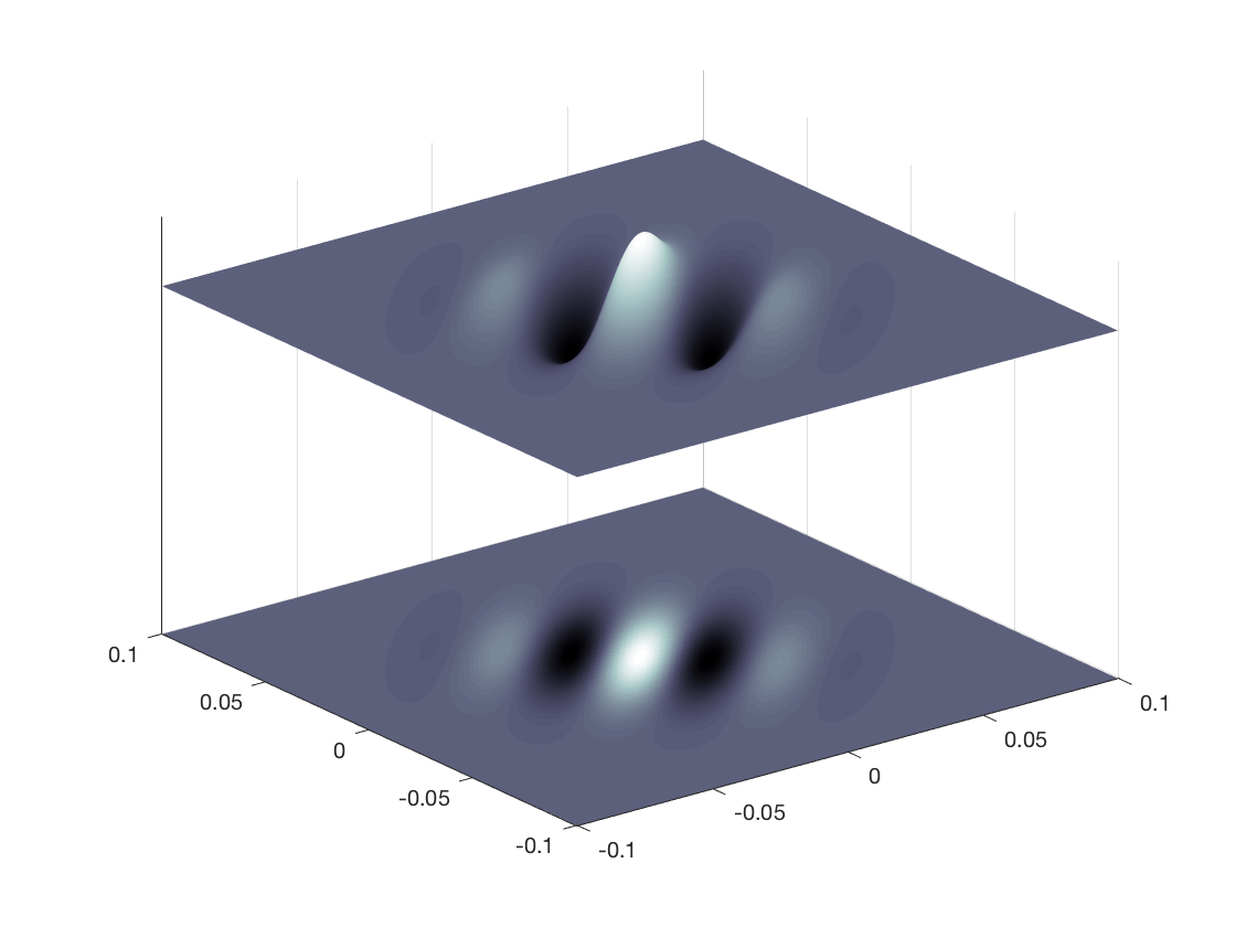
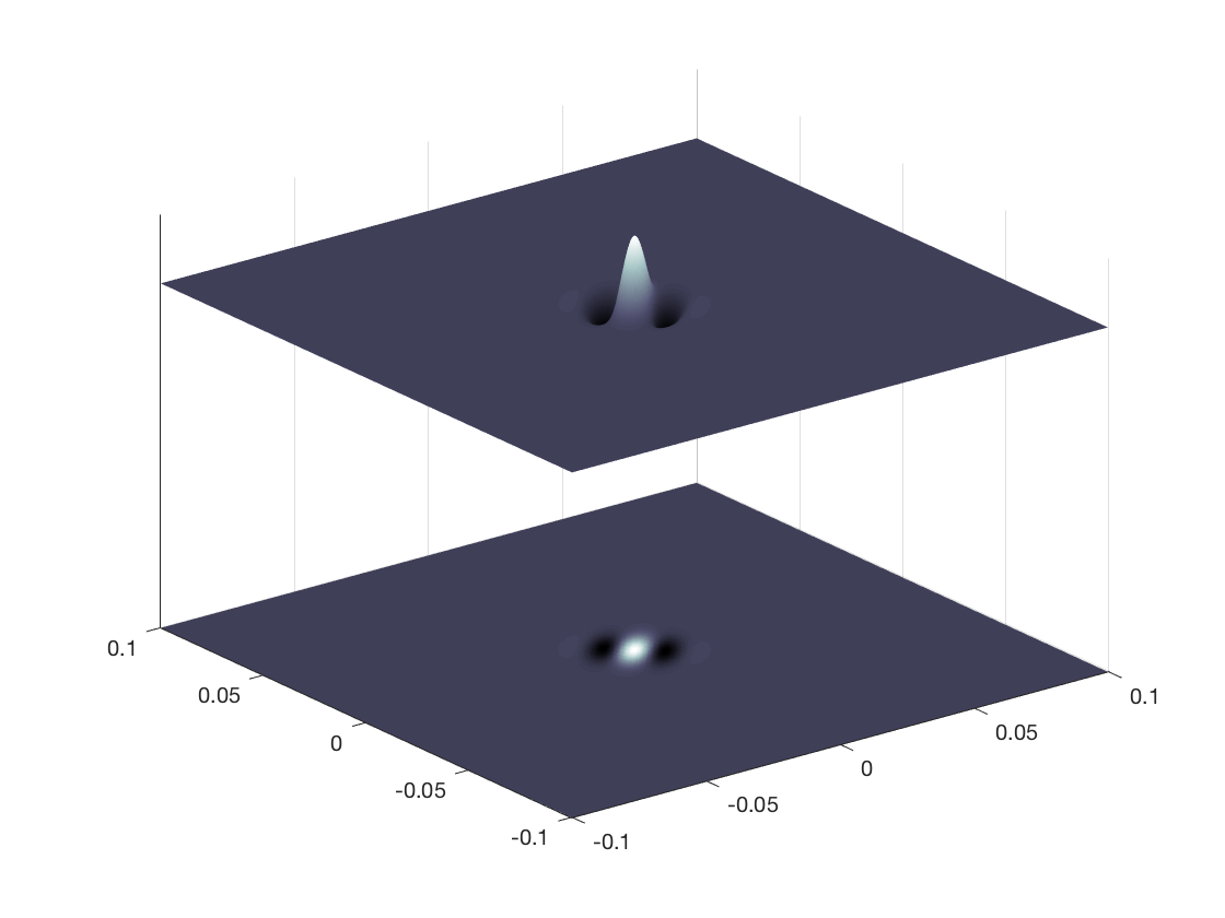
Figure 2.2. On the left, the space profile and contour plot of a frame element with $j=2$. On the right, the same plot with a Gaussian window contracted by a factor of $2\pi\ln(16)$, which is better adapted for certain numerical examples. See Appendix E.

Although we are mainly interested in high frequency expansions: $\sum_{\gamma\in\Gamma}f_{\gamma}\varphi_{\gamma}$, in order to expand an arbitrary function we need to provide wavepackets adapted to the zeroth-scale. To keep the notation concise, we let $\varphi_{0,0}:=\varphi$, augment the index set $\Gamma$ by

(2.6) $$\Gamma_{*}:=\Gamma\cup\{(0,0,\lambda):\lambda\in\Lambda\},$$

and define zeroth-scale wavepackets as: $\varphi_{0,0,\lambda}:=\varphi(x-\lambda)$. The complete set of wavepackets can be written as:

$$\mathcal{F}=\left\{\varphi_{\gamma}:\gamma\in\Gamma_{*}\right\}.$$

We now show that the system thus constructed is indeed rich enough to represent any function.

Theorem 2.1.

For an adequate lattice $\Lambda\subseteq{\mathbb{R}^{d}}$, the system $\mathcal{F}$ is a frame for the inhomogeneous Sobolev spaces $H^{s}({\mathbb{R}^{d}})$, with $-1\leq s\leq 1$. More precisely, the frame operator

(2.7) $${S_{\mathcal{F}}}f=\sum_{\gamma\in\Gamma_{*}}\left<f,\varphi_{\gamma}\right>\varphi_{\gamma}$$

is invertible on $H^{s}({\mathbb{R}^{d}})$ for $-1\leq s\leq 1$. In addition, we have the norm equivalence

(2.8) $$\lVert f\rVert_{H^{s}}^{2}\asymp\sum_{\gamma\in\Gamma_{*}}4^{2js}\left|\left<f,\varphi_{\gamma}\right>\right|^{2}.$$

We remark that in (2.7) and (2.8) the symbol $\left<f,\varphi_{\gamma}\right>$ denotes the standard $L^{2}$ inner product. The theorem is proved using a variant of Daubechies’s criterion for wavelets. Details are provided in Appendix D. The construction provides a concrete criterion to choose the lattice $\Lambda$ and $A\lVert f\rVert_{H^{s}}\leq\lVert{S_{\mathcal{F}}}f\rVert_{H^{s}}\leq B\lVert f\rVert_{H^{s}}$ can be satisfied with $B/A$ reasonably small (see Figure 4.7). Hence, the numerical inversion of ${S_{\mathcal{F}}}$ is well-conditioned.

From now on we fix a lattice $\Lambda$ such that the conclusion of Theorem 2.1 holds.

As a consequence of Theorem 2.1, every $f\in H^{s}({\mathbb{R}^{d}})$ can be represented by an $H^{s}$-convergent series

(2.9) $$f=\sum_{\gamma\in\Gamma_{*}}f_{\gamma}\varphi_{\gamma},\qquad\mbox{with }f_{\gamma}:=\left<f,{S_{\mathcal{F}}}^{-1}\varphi_{\gamma}\right>,$$

and

$$\lVert f\rVert^{2}_{H^{s}}\asymp\lVert{S_{\mathcal{F}}}^{-1}f\rVert^{2}_{H^{s}}\asymp\sum_{\gamma\in\Gamma_{*}}4^{2js}\left|f_{\gamma}\right|^{2}.$$

2.2. Operating on the frame expansion

We will be mostly interested in the higher scales $j\geq 1$. We can truncate the representation in (2.9),

(2.10) $$\tilde{f}=\sum_{\gamma\in\Gamma}f_{\gamma}\varphi_{\gamma},$$

and it is easy to see that the error can be bounded as

(2.11) $$\lVert f-\tilde{f}\rVert_{H^{1}}\lesssim\lVert f\rVert_{H^{-1}}.$$

Hence, in the highly oscillatory regime, we only need to consider expansions of the form (2.10).

More generally, we use pseudodifferential cut-offs to operate microlocally on a function $f$ and we wish to approximately implement those operations by acting directly on the expansion in (2.10). We recall that a symbol $\sigma:{\mathbb{R}^{d}}\times{\mathbb{R}^{d}}\to\mathbb{C}$ belongs to the Hörmander class $S^{0}_{1,0}({\mathbb{R}^{d}}\times{\mathbb{R}^{d}})$ if

$$\left|\partial_{x}^{\beta}\partial_{\xi}^{\alpha}\sigma(x,\xi)\right|\leq C_{\alpha,\beta}(1+\left|\xi\right|)^{-\left|\alpha\right|},$$

for all multi-indices $\alpha,\beta$. The next lemma will be an important technical tool, and is proved in more generality in Appendix C.

Theorem 2.2.

Let $\sigma\in S^{0}_{1,0}({\mathbb{R}^{d}}\times{\mathbb{R}^{d}})$. Then, for $s\in[1/2,1]$ and $f\in H^{s}({\mathbb{R}^{d}})$,

(2.12) $$\lVert\sigma(x,D)f-\sum_{\gamma\in\Gamma}\sigma(2^{-j}\lambda,\xi_{j,k})f_{\gamma}\varphi_{\gamma}\rVert_{H^{s}}\lesssim\lVert f\rVert_{H^{s-1/2}}.$$

(Here, $\sigma(x,D)$ is the Kohn-Nirenberg quantization of $\sigma$, and $f_{\gamma}:=\left<f,{S_{\mathcal{F}}}^{-1}\varphi_{\gamma}\right>$ are the high-scale frame coefficients of $f$.)

2.3. Gaussian Beams

We summarize the construction of Gaussian beams, following the treatment of Katchalov, Kurylev and Lassas [26]. Consider the wave equation,

(2.13) $$\begin{split}\partial_{t}^{2}u(t,x)-c^{2}(x)\Delta_{x}u(t,x)&{}=0\end{split}$$

with $c\in C^{\infty}(\mathbb{R}^{d})$ (strictly) positive with bounded derivatives of all orders. We seek formal asymptotic solutions (in a “moving” frame of reference) of the form

(2.14) $$\Phi(t,x)=A(t,x)e^{i\omega\theta(t,x)},$$

where the phase function $\theta$ and amplitude function $A$ are smooth complex-valued functions of $(t,x)$, and $\omega$ is the frequency parameter. Substituting this asymptotic trial solution into the wave equation, and extracting the leading order terms in $\omega$, one finds the eikonal and transport equations,

(2.15) $$(\partial_{t}\theta)^{2}-c|\nabla_{x}\theta|^{2} {}=0,$$

(2.16) $$2\partial_{t}A\,\partial_{t}\theta-2c^{2}\nabla_{x}A\cdot\nabla_{x}\theta+A\,(\partial_{t}^{2}\theta-c^{2}\operatorname{Tr}(\Delta_{x}\theta)) {}=0.$$

We factorize the eikonal equation into

(2.17) $$\partial_{t}\theta^{\pm}+H^{\pm}(x,\nabla_{x}\theta^{\pm})=0,$$

where $\theta^{\pm}$ corresponds to positive and negative frequencies respectively, and

(2.18) $$H^{\pm}(x,p)=\pm c(x)|p|,$$

are the signed Hamiltonians. The propagation of singularities of solutions to the wave equation is described by the bicharacteristics, $x^{\pm}(t)$, $p^{\pm}(t)$, satisfying the Hamilton system

(2.19) $$\dot{x}^{\pm}(t)=\phantom{-}\partial_{p}H^{\pm},\quad\dot{p}^{\pm}(t)=-\partial_{x}H^{\pm},$$

supplemented with initial conditions, $x^{\pm}(0)=x_{0}$, $p^{\pm}(0)=p_{0}$. For the sake of simplicity, we drop the superscript $\pm$ when we do not need to differentiate the two solutions. In particular, $H$ denotes either $H^{+}$ or $H^{-}$.

A Gaussian beam is a solution of the type (2.14), the phase function of which is assumed to satisfy the conditions,

(2.20) $$\Im\theta(t,x(t)) {}=0,$$

(2.21) $$\Im\theta(t,x) {}\geq F_{0}(t)\left|x-x(t)\right|^{2},$$

where $F_{0}(t)$ is a continuous positive function. To construct such a solution, one expands the phase function to second order,

(2.22) $$\theta(t,x)=\theta_{0}(t)+p(t)\cdot(x-x(t))+\tfrac{1}{2}(x-x(t))^{T}M(t)(x-x(t)),$$

and the amplitude function to zero order,

(2.23) $$A(t,x)=A(t,x(t))=A(t).$$

The phase function along the characteristic $\theta_{0}(t)=\theta(t,x(t))$ satisfies

$$\dot{\theta_{0}}(t)=(\partial_{t}\theta)(t,x(t))+p(t)\cdot(\partial_{p}H)(t,x(t)))=0$$

in view of the homogeneity of $H$; hence, $\theta_{0}(t)$ can be taken to be zero.

The matrix $M$ satisfies the Riccati equation,

(2.24) $$\dot{M}(t)+D(t)+B(t)M(t)+M(t)B(t)^{t}+M(t)X(t)M(t)=0,$$

where $B(t),X(t),D(t)$ are $d\times d$ matrices with elements given by the second-order derivatives of the Hamiltonian,

$$D_{ij}(t)=\partial_{x_{i}}\partial_{x_{j}}H,\quad B_{ij}(t)=\partial_{x_{i}}\partial_{p_{j}}H,\quad X_{ij}(t)=\partial_{p_{i}}\partial_{p_{j}}H,$$

evaluated along the bicharacteristic $(x,p)=(x(t),p(t))$. The Riccati equation is supplemented with the initial condition $M(0)=M_{0}$. The symplectic structure of the Hamilton system implies that $M(t)$ is symmetric and has a positive definite imaginary part provided that it initially does (see Lemma 2.8 and [26, Lemma 2.56]).

The amplitude function $A$ satisfies the transport equation

(2.25) $$\dot{A}(t)+\frac{A(t)}{2H}\left(\mbox{\rule{0.0pt}{12.80365pt}}\right.c^{2}\operatorname{Tr}(M(t))-\partial_{p}H\cdot\partial_{x}H-(\partial_{p}H)^{T}M(t)\,\partial_{p}H\left.\mbox{\rule{0.0pt}{12.80365pt}}\right)=0,$$

where $H$ and its derivatives are evaluated along the bicharacteristic $(x,p)=(x(t),p(t))$. This equation is supplemented with the initial condition $A(0)=A_{0}$. We find solutions, $M(t)=M^{\pm}(t)$ and $A(t)=A^{\pm}(t)$; the latter can written as

(2.26) $$A(t)=\frac{A_{0}}{|\det Y(t)|^{1/2}}\ \exp\left(\int_{0}^{t}\operatorname{Tr}[X(x(s),p(s)]\,ds\right)$$

with

$$\dot{Y}(t)-B^{t}Y(t)-XMY(t)=0\quad\text{and}\quad Y_{0}=I,$$

see [46, Lemma 6.3] for details.

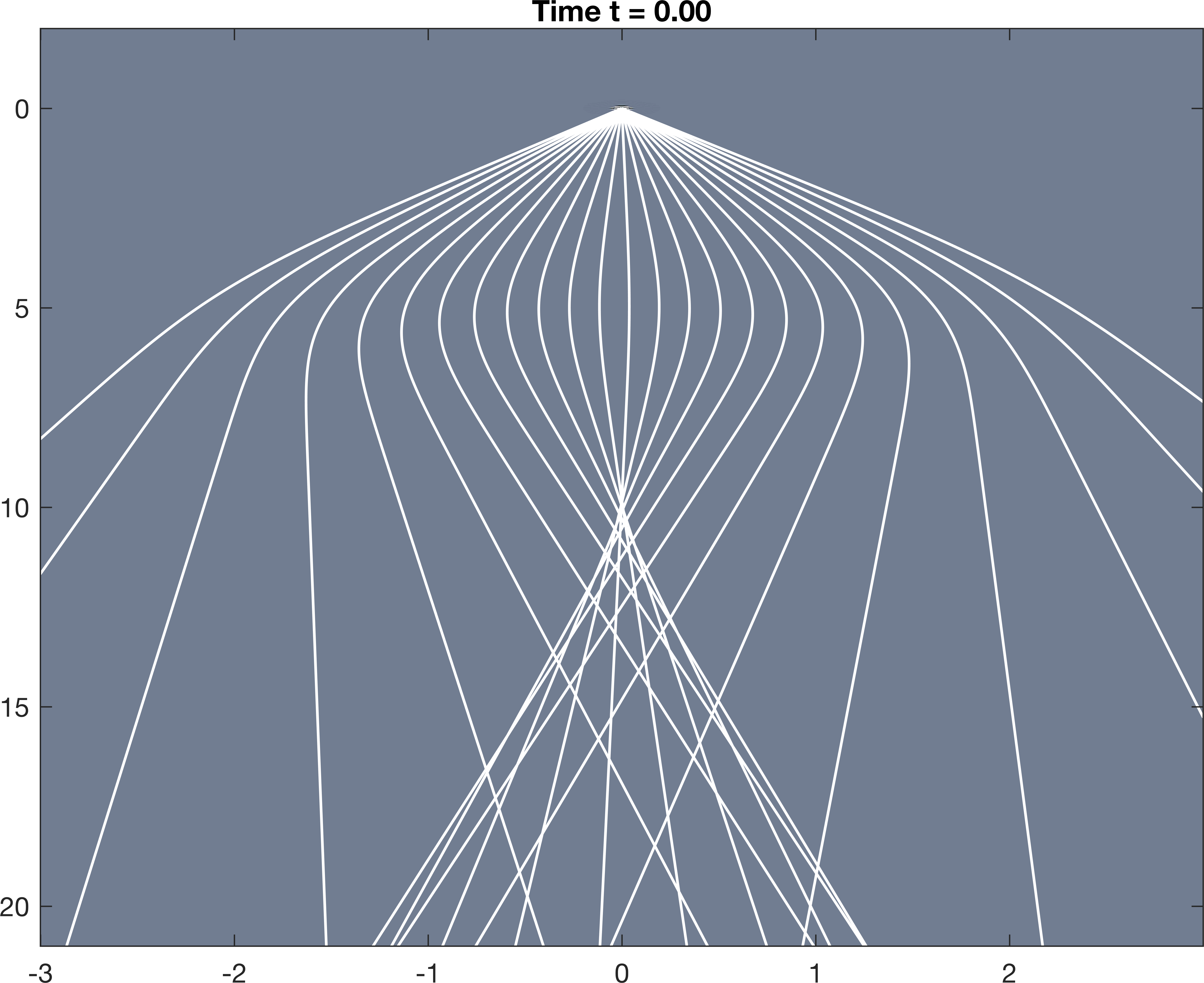
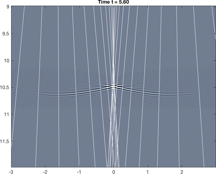
Figure 2.3. The projected characteristics corresponding to the velocity $c(x_{1},x_{2})=2-0.4*\exp{(-(x_{1}^{2}+(x_{2}-5)^{2})/3)}$, and a detail of the evolution of a front of Gaussian packets. Initially localized on the boundary, the front goes through a caustic at time $t\approx 5.60$. See Appendix E.

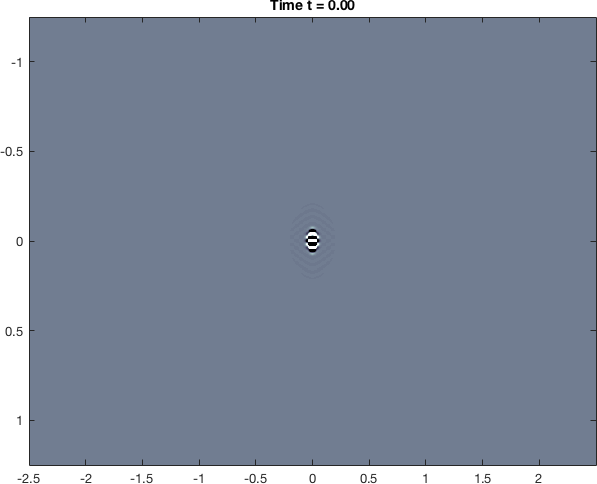
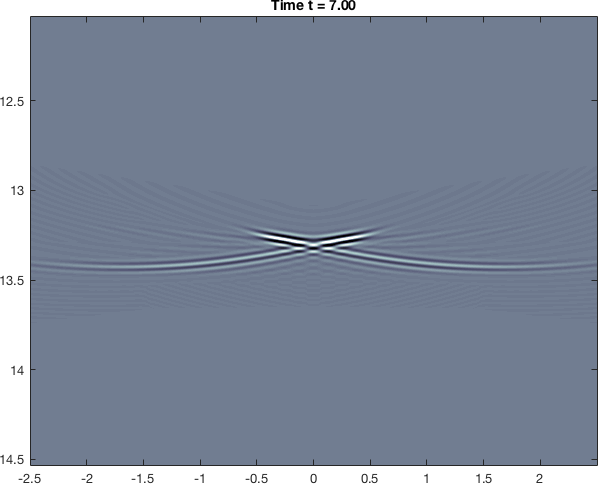
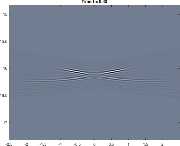
Figure 2.4. Detailed evolution of the wavefront corresponding to Figure 2.3.

In what follows, we discuss families of Gaussian beams, with the goal of describing superimpositions and time evolution. See Figures 2.3 and 2.4 for plots of a front of Gaussian beams going through a caustic, and Appendix E for details on the example.

2.4. Sets of initial conditions for Gaussian beams

We consider families of Gaussian beams associated with sets of parameters described as follows. We let $\Gamma_{0}$ be a subset of $\Gamma$ and $\mathcal{S}$ be a map

(2.27) $$\mathcal{S}_{\gamma}=(\omega_{\gamma},a_{\gamma},\xi_{\gamma},\mathcal{A}_{\gamma},\mathcal{M}_{\gamma})\in\mathbb{R}_{+}\times{\mathbb{R}^{d}}\times({\mathbb{R}^{d}}\setminus\left\{0\right\})\times(\mathbb{R}\setminus\{0\})\times\mathbb{C}^{d\times d},\qquad\gamma\in\Gamma_{0},$$

such that $\mathcal{M}_{\gamma}$ is symmetric and $\Im\mathcal{M}_{\gamma}>0$ for all $\gamma\in\Gamma_{0}$. We associate two functions $\Phi^{+}_{\gamma},\Phi^{-}_{\gamma}:\mathbb{R}\times{\mathbb{R}^{d}}\to\mathbb{C}$ that we now describe. To simplify the notation we drop the superscript $+$,$-$. Let $x_{\gamma}(t)$, $p_{\gamma}(t)$, $M_{\gamma}(t)$, $A_{\gamma}(t)$ be the solutions to the set of ODEs defined in (2.19), (2.24) and (2.25), supplemented with initial conditions:

(2.28) $$x|_{t=0}=a_{\gamma},$$

(2.29) $$p|_{t=0}=2\pi\frac{\xi_{\gamma}}{\omega_{\gamma}},$$

(2.30) $$M|_{t=0}=2\pi\mathcal{M}_{\gamma},$$

(2.31) $$A|_{t=0}=\mathcal{A}_{\gamma}{\omega_{\gamma}}^{\frac{d}{4}}.$$

We now define the beams by

(2.32) $$\Phi_{\gamma}(t,x)=A_{\gamma}(t)e^{i\omega_{\gamma}\theta_{\gamma}(t,x)},$$

with

(2.33) $$\theta_{\gamma}(t,x)=p_{\gamma}(t)\cdot(x-x_{\gamma}(t))+\tfrac{1}{2}(x-x_{\gamma}(t))\cdot M_{\gamma}(t)(x-x_{\gamma}(t)).$$

The ODEs in (2.19), (2.24) and (2.25) have globally defined unique solutions for the initial conditions given by (2.28)-(2.31). Indeed, the system of ODEs in (2.19) is the flow associated with the Hamiltonian $H$ and, due to the homogeneity of $H(x,p)$ in $p$, it is solvable as long as the initial condition $p|_{t=0}$ is non-zero. That is why we require that $\xi_{\gamma}\not=0$. Once the Hamiltonian flow $(x,p)$ is defined, (2.24) has a globally defined unique solution because the initial datum is symmetric and has a positive imaginary part [26, Lemma 2.56]. Finally, (2.25) has also a unique global solution, since it is a linear ODEs with continuous coefficients.

Remark 2.3.

When we need to emphasize the dependence on the choice of sign for $H$ we write: $\Phi^{\pm}_{\gamma}$, $x_{\gamma}^{\pm}(t),p_{\gamma}^{\pm}(t),M_{\gamma}^{\pm}(t),A_{\gamma}^{\pm}(t)$. We stress that these functions depend not only on the index $\gamma$, but also on the underlying map from (2.27), that describes how to associate with $\gamma$ initial conditions for the ODEs defining the beam. When we need to stress this dependence we use further superscripts.

Remark 2.4.

By abuse of language, we often refer to a set of GB parameters $\Upsilon=\left\{\mathcal{S}_{\gamma}:\gamma\in\Gamma_{0}\right\}$, although it is not the set $\Upsilon$, but the underlying map $\mathcal{S}$ that matters. Hence, $\Upsilon$ should be considered as an indexed set, that is formally equivalent to the map $\mathcal{S}$.

2.5. Standard initial conditions

We now describe the canonical set of GB parameters, defined so that the corresponding Gaussian beams at time $t=0$ coincide with the higher-scale part of the frame $\mathcal{F}$. We define the standard set of Gaussian beam parameters as the set $\Upsilon^{st}=\left\{\mathcal{S}^{st}_{\gamma}:\gamma\in\Gamma\right\}$ given by

(2.34) $$\mathcal{S}^{st}_{\gamma}=(4^{j},2^{-j}\lambda,\xi_{j,k},2^{\frac{d}{4}},iI_{d}),\qquad\gamma=(j,k,\lambda)\in\Gamma.$$

The corresponding beams are denoted $\{\Phi^{{\rm st},\pm}_{\gamma}:\gamma\in\Gamma\}$.

Observation 2.5.

For the standard set of parameters $\Upsilon^{st}$:

$$\Phi^{{\rm st},\pm}_{\gamma}(0,x)=\varphi_{j,k,\lambda}(x),\qquad\gamma=(j,k,\lambda)\in\Gamma.$$

This follows by substituting (2.34) into (2.28)-(2.31) and (2.32)-(2.33).

2.6. Properties of the defining ODEs

We now show that certain uniformity properties of a family of Gaussian beams parameters imply corresponding uniformity properties for the ODEs defining the beams.

Lemma 2.6.

Let $\{\mathcal{S}_{\gamma}:\gamma\in\Gamma_{0}\}$ be a set of GB parameters. Assume that there exist $0<C_{0}\leq C_{1}$ such that $C_{0}\left|\xi_{\gamma}\right|\leq\omega_{\gamma}\leq C_{1}\left|\xi_{\gamma}\right|$. Let $T>0$. Then the following estimates hold for $\gamma,\gamma^{\prime}\in\Gamma_{0}$ and $t\in[-T,T]$:

(2.35) $$|a_{\gamma}-a_{\gamma^{\prime}}|^{2}\leq|x_{\gamma}(t)-x_{\gamma^{\prime}}(t)|^{2}+C_{T},\>|x_{\gamma}(t)-x_{\gamma^{\prime}}(t)|^{2}\leq|a_{\gamma}-a_{\gamma^{\prime}}|^{2}+C_{T},$$

(2.36) $$|p_{\gamma}(t)|\asymp|p_{\gamma}(0)|\asymp 1,$$

(2.37) $$|\dot{x}_{\gamma}(t)|,|\dot{p}_{\gamma}(t)|\lesssim 1,$$

(2.38) $$d\Big{(}\big{(}x_{\gamma}(t),\omega_{\gamma}p_{\gamma}(t)\big{)},\big{(}x_{\gamma^{\prime}}(t),\omega_{\gamma^{\prime}}p_{\gamma^{\prime}}(t)\big{)}\Big{)}\asymp d\Big{(}\big{(}a_{\gamma},\xi_{\gamma}\big{)},\big{(}a_{\gamma^{\prime}},\xi_{\gamma^{\prime}}\big{)}\Big{)},$$

where the constant $C_{T}$ and the implied constants depend on $T$, $C_{0}$ and $C_{1}$ but not on the particular pair of parameters $\gamma,\gamma^{\prime}$.

Proof.

The bounds (2.35) and (2.36) follow from the assumptions on the velocity and Gronwall’s lemma; see the proofs of [6, Lemmas 3.1 and 3.3]. Using the equations for the Hamiltonian flow, the assumptions on $c$, and (2.35) we get

$$\left|\dot{x}_{\gamma}(t)\right|=\left|c(x(t))\right|\leq C,$$

$$\left|\dot{p}_{\gamma}(t)\right|=\left|\nabla{c}(x(t))\right|\left|p(t)\right|\lesssim C,$$

where $C$ is a constant that depends only on the velocity $c$. This gives (2.37). Finally, the estimate in (2.38) is proved in [6, Lemma 3.2]. ∎

Remark 2.7.

In Lemma 2.6, the conclusion $\left|p_{\gamma}(t)\right|\asymp 1$ holds because the initial condition associated with $\gamma$ in (2.29) ensures that $\left|p_{\gamma}(0)\right|\asymp 1$, with the assumption that $\left|\xi_{\gamma}\right|\asymp\omega_{\gamma}$. In general, if $(x,p)$ is the flow associated with $H^{+}$ or $H^{-}$ with arbitrary initial conditions, it follows from our assumptions in the velocity that $\left|p(t)\right|\asymp\left|p(0)\right|$ with constants that are uniform on any bounded interval of time.

For more particular initial conditions, the following further properties hold.

Lemma 2.8.

Let $\{\mathcal{S}_{\gamma}:\gamma\in\Gamma_{0}\}$ be a set of GB parameters. Assume that there exist constants $0<C_{0}\leq C_{1}$ such that for all $\gamma\in\Gamma_{0}$: $\lVert\mathcal{M}_{\gamma}\rVert\leq C_{1}$, $\Im{\mathcal{M}_{\gamma}}\geq C_{0}\cdot I_{d}$, and $C_{0}\left|\xi_{\gamma}\right|\leq\omega_{\gamma}\leq C_{1}\left|\xi_{\gamma}\right|$. Let $T\geq 0$. Then there exist constants $C_{0}^{\prime},C_{1}^{\prime}>0$ - that only depend on $T$, $C_{0}$ and $C_{1}$ - such that the following estimates hold for $t\in[-T,T]$:

(2.39) $$\lVert M_{\gamma}(t)\rVert\leq C_{1}^{\prime},$$

(2.40) $$\Im M_{\gamma}(t)\geq C_{0}^{\prime}\cdot I_{d},$$

(2.41) $$C_{0}^{\prime}\left|\mathcal{A}_{\gamma}\omega_{\gamma}^{\frac{d}{4}}\right|\leq\left|A_{\gamma}(t)\right|\leq C_{1}^{\prime}\left|\mathcal{A}_{\gamma}\omega_{\gamma}^{\frac{d}{4}}\right|.$$

Proof.

Consider the matrix-valued ODE in (2.24). The derivatives of the Hamiltonian $H(x,p)$ are bounded on any set where $\left|p\right|$ is bounded above and below. Since $\left|p_{\gamma}(t)\right|$ is bounded above and below on $[-T,T]$ by Lemma 2.6, it follows that the coefficients in (2.24) are bounded. In addition, the norm of the initial condition $M_{\gamma}(0)=\mathcal{M}_{\gamma}$ is bounded by assumption - cf. (2.30). Therefore, (2.39) follows by Gronwall’s lemma. The estimate in (2.41) now follows from [6, Lemma 3.1] (which requires $\lVert M(t)\rVert$ to be bounded). Finally, (2.40) is proved in [26, Lemma 2.56]. The statement there is non-quantitative, but the argument gives the desired conclusion. See also [6, Lemma 3.4]. ∎

3. Well-spread families of Gaussian Beam parameters

3.1. Definitions

We develop criteria under which a family of Gaussian beam parameters behaves qualitatively like the standard one, given by

$$\mathcal{S}^{st}_{\gamma}=(\omega^{st}_{\gamma},a^{st}_{\gamma},\xi^{st}_{\gamma},\mathcal{A}^{st}_{\gamma},\mathcal{M}^{st}_{\gamma})=(4^{j},2^{-j}\lambda,\xi_{j,k},2^{\frac{d}{4}},iI_{d}),\qquad\gamma=(j,k,\lambda).$$

Our main goal is to show that when an adequate family of parameters is used as initial values, then a linear combination of the corresponding Gaussian beams satisfies a suitable Bessel bound and provides an approximate solution to the wave equation.

Definition 3.1.

A well-spread set of Gaussian beam parameters is an indexed set

$$\Upsilon\equiv\left\{\mathcal{S}_{\gamma}:\gamma\in\Gamma_{0}\right\}\subseteq\mathbb{R}_{+}\times{\mathbb{R}^{d}}\times({\mathbb{R}^{d}}\setminus\left\{0\right\})\times(\mathbb{R}\setminus\{0\})\times\mathbb{C}^{d\times d},\qquad\gamma\in\Gamma_{0}$$

with $\Gamma_{0}\subseteq\Gamma$, such that

• $|a^{st}_{\gamma}-a^{st}_{\gamma^{\prime}}|\lesssim|a_{\gamma}-a_{\gamma^{\prime}}|+1,\qquad\gamma,\gamma^{\prime}\in\Gamma_{0}$.

• $d((a_{\gamma},\xi_{\gamma}),(a_{\gamma^{\prime}},\xi_{\gamma^{\prime}}))\gtrsim d((a^{st}_{\gamma},\xi^{st}_{\gamma}),(a^{st}_{\gamma^{\prime}},\xi^{st}_{\gamma^{\prime}})),\qquad\gamma,\gamma^{\prime}\in\Gamma_{0}$.

• $\mathcal{M}_{\gamma}\in\mathbb{C}^{d\times d}$ is symmetric, $\lVert\mathcal{M}_{\gamma}\rVert\lesssim 1$ and $\Im(\mathcal{M}_{\gamma})\gtrsim I_{d}$, $\qquad\gamma\in\Gamma_{0}$.

• $\omega_{\gamma}\asymp 4^{j}$ and $\left|\xi_{\gamma}\right|\asymp\omega_{\gamma}$, $\qquad\gamma\in\Gamma_{0}$.

• $|\mathcal{A}_{\gamma}|\asymp 1$, $\qquad\gamma\in\Gamma_{0}$.

In the last definition, the symbols $\lesssim$, $\gtrsim$ and $\asymp$ should be interpreted as asserting the existence of suitable constants that are uniform within the family $\Upsilon$.

Remark 3.2.

For short, we say that $\{\Phi^{+}_{\gamma}:\gamma\in\Gamma_{0}\}$ and $\{\Phi^{-}_{\gamma}:\gamma\in\Gamma_{0}\}$ are well-spread families of Gaussian beams, implying the existence of a corresponding well-spread family of Gaussian beam parameters $\Upsilon\equiv\left\{\mathcal{S}_{\gamma}:\gamma\in\Gamma_{0}\right\}$ that defines the beams.

Similarly, when a certain family of GB parameters $\Upsilon$ is discussed, we may denote the corresponding beams by just $\Phi^{\pm}_{\gamma}$, without remarking their dependence on the map $\mathcal{S}$.

Before proving the main estimates, we define an adequate notion of vanishing order along a family of Gaussian beams.

Definition 3.3.

Given a well-spread set of GB parameters $\Upsilon\equiv\left\{\mathcal{S}_{\gamma}:\gamma\in\Gamma_{0}\right\}$, an interval $I\subseteq\mathbb{R}$, and $m\in\mathbb{N}_{0}$, a family of functions $F\equiv\left\{F_{\gamma}:\gamma\in\Gamma_{0}\right\}$ is said to be $F={\mathbb{O}}^{m}(I,\Upsilon)$ if

• $F_{\gamma}(t,x)=\sum_{\left|\eta\right|={m}}G_{\gamma,\eta}(t,x)(x-x_{\gamma}(t))^{\eta}$, for some functions $G_{\gamma,\eta}(t,\cdot)\in C^{\infty}_{b}({\mathbb{R}^{d}})$, for all $t\in I$.

• $\sup_{\gamma\in\Gamma_{0},t\in I}\lVert\partial^{k}G_{\gamma,\eta}(t,\cdot)\rVert_{L^{\infty}({\mathbb{R}^{d}})}<+\infty$, for all multi-indices $k$ and $\eta$, with $\left|\eta\right|=m$.

Thus, $F={\mathbb{O}}^{m}(I,\Upsilon)$ means that each $F_{\gamma}(t,\cdot)=O(\left|x-x_{\gamma}(t)\right|^{m},{\mathbb{R}^{d}})$ and the corresponding bounds are uniform for $t\in I$ and $\gamma\in\Gamma_{0}$.

We note that the definition of ${\mathbb{O}}^{m}(I,\Upsilon)$ involves a vanishing condition at $x=x_{\gamma}(t)$ and also a growth condition for $\left|x-x_{\gamma}(t)\right|\gg 1$. As a consequence, $F={\mathbb{O}}^{m+1}(I,\Upsilon)$ does not imply $F={\mathbb{O}}^{m}(I,\Upsilon)$. As a remedy, we introduce the following notion.

Definition 3.4.

Given a well-spread set of GB parameters $\Upsilon\equiv\left\{\mathcal{S}_{\gamma}:\gamma\in\Gamma_{0}\right\}$ and an interval $I\subseteq\mathbb{R}$, a family of functions $F\equiv\left\{F_{\gamma}:\gamma\in\Gamma_{0}\right\}$ is said to be $F=\mathbb{O}_{\geq}^{m}(I,\Upsilon)$ if there exists a finite family $F^{1}={\mathbb{O}}^{m_{1}}(I,\Upsilon),\ldots,F^{n}={\mathbb{O}}^{m_{n}}(I,\Upsilon)$, with $m_{1},\ldots,m_{n}\geq m$, such that $F_{\gamma}(t,x)=F^{1}_{\gamma}(t,x)+\ldots+F^{n}_{\gamma}(t,x)$.

Note that $F=\mathbb{O}_{\geq}^{m+1}(I,\Upsilon)$ implies that $F=\mathbb{O}_{\geq}^{m}(I,\Upsilon)$.

3.2. Bessel bounds and vanishing orders

We prove a Bessel bound for the summation of Gaussian beams with factors vanishing at the spatial center of the beams. This extends the result obtained in [6, Sec. 3] from $L^{2}(\mathbb{R}^{d})$ to Sobolev spaces, and to more general sets of initial conditions.

Theorem 3.5.

Let $\Upsilon=\left\{\mathcal{S}_{\gamma}:\gamma\in\Gamma_{0}\right\}$ be a well-spread set of Gaussian beam parameters and let $F=\mathbb{O}_{\geq}^{m}(I,\Upsilon)$, with $I\subseteq\mathbb{R}$ a bounded interval and $s\in[0,1]$. Then

$$\sup_{t\in I}\Big{\|}\sum_{\gamma\in\Gamma_{0}}2^{jm}b_{\gamma}\Phi^{\pm}_{\gamma}(t,\cdot)F_{\gamma}(t,\cdot)\Big{\|}^{2}_{H^{s}}\lesssim C_{I}\sum_{\gamma\in\Gamma_{0}}4^{2sj}|b_{\gamma}|^{2},$$

with $b_{\gamma}\in\mathbb{C}$ such that the sum on the right-hand side is finite. (Here, the constant $C_{I}$ depends on the interval $I$ and the family $F$.)

Proof.

Without loss of generality we may assume that $F={\mathbb{O}}^{m}(I,\Upsilon)$. According to Definition 3.3,

$$F_{\gamma}(t,x)=\sum_{\left|\eta\right|={m}}G_{\gamma,\eta}(t,x)(x-x_{\gamma}(t))^{\eta}$$

for some adequate functions $G_{\gamma,\eta}(t,\cdot)\in C^{\infty}_{b}({\mathbb{R}^{d}})$.

The estimates relevant for the Bessel bounds are developed in greater generality in Appendix B. Indeed, Lemma B.1 implies that the beams $\{\Phi^{\pm}_{\gamma}(t,\cdot):\gamma\in\Gamma_{0}\}$ are sets of wave-molecules uniformly for $t\in I$ (see Appendix B for the definitions). Second, the multiplication operators have symbols $G_{\gamma,\eta}(t,\cdot)$ that belong to the Hörmander class $S^{0}_{1,0}$ uniformly for $t\in I$ and $\gamma\in\Gamma_{0}$. Hence, using Lemmas B.3 and B.4 we conclude that $\{2^{jm}F_{\gamma}(t,\cdot)\Phi^{\pm}_{\gamma}:\gamma\in\Gamma_{0}\}$ is a set of wave-molecules uniformly for $t\in I$, and, by Lemma B.5, it satisfies the desired Bessel bounds. ∎

Remark 3.6.

The choice $I=\left\{0\right\}$ is allowed in Theorem 3.5 and corresponds to time-independent functions $F_{\gamma}(x)=F_{\gamma}(0,x)$. Since, for the standard set of GB parameters, the beams at time $t=0$ coincide with the higher-scale frame elements - cf. Observation  2.5 - we conclude that, given $F_{\gamma}=\mathbb{O}_{\geq}^{m}(\{0\},\Upsilon^{\textrm{st}})$,

$$\Big{\|}\sum_{\gamma\in\Gamma}2^{jm}b_{\gamma}\varphi_{\gamma}F_{\gamma}\Big{\|}^{2}_{H^{s}}\lesssim\sum_{\gamma\in\Gamma}4^{2js}|b_{\gamma}|^{2},\qquad s\in[0,1].$$

3.3. Uniformity of errors for Taylor expansions

Most of our arguments rely on Taylor expansions for the functions $x,p,A,M$ used in the definition of Gaussian beams. The following lemma is used to justify that, in such arguments, the error terms can be bounded uniformly within a given well-spread family of Gaussian beams.

Lemma 3.7.

Let $\Upsilon=\left\{\mathcal{S}_{\gamma}:\gamma\in\Gamma_{0}\right\}$ be a well-spread set of Gaussian beam parameters, let $T\geq 0$ and $k\geq 0$ be an integer. Then the following quantities:

$$\sup_{\gamma\in\Gamma_{0}}\sup_{t\in[-T,T]}\left|\partial^{k+1}_{t}x_{\gamma}(t)\right|, \qquad\sup_{\gamma\in\Gamma_{0}}\sup_{t\in[-T,T]}\left|\partial^{k}_{t}p_{\gamma}(t)\right|,$$

$$\sup_{\gamma\in\Gamma_{0}}\sup_{t\in[-T,T]}\left|\partial^{k}_{t}M_{\gamma}(t)\right|,$$

are bounded by a constant that depends on $T$, $k$ and $\Upsilon$. In addition,

(3.1) $$\partial_{t}A_{\gamma}(t)=A_{\gamma}(t)G_{\gamma}(t),$$

with $\displaystyle\sup_{\gamma\in\Gamma_{0}}\sup_{t\in[-T,T]}\left|\partial^{k}_{t}G_{\gamma}\right|$ bounded by a constant that depends on $T$, $k$ and $\Upsilon$.

Proof.

Since the derivatives of the velocity $c$ are bounded, the derivatives of $H(x,p)$ are bounded on any set where $\left|p\right|$ is bounded above and below. By Lemma 2.6, $\left|p_{\gamma}(t)\right|\asymp 1$ and, therefore, we conclude that

(3.2) $$\sup_{t\in[-T,T]}\left|\partial^{n}_{x}\partial^{m}_{p}H(x_{\gamma}(t),p_{\gamma}(t))\right|\lesssim C_{n,m,T}<\infty,$$

for all multi-indices $n,m$. Inspecting the definition of the Hamiltonian field $(x_{\gamma},p_{\gamma})$ - cf. (2.19), the claim on $x$ and $p$ follows from (3.2).

For the matrix $M_{\gamma}$, we note that, due to (3.2), it satisfies a Riccati-type ODE where the coefficients are bounded and have all the derivatives bounded. Moreover, the corresponding initial condition is bounded, as part of Definition 3.1. Hence, the claim on $M_{\gamma}$ follows from a Gronwall-type argument for linear systems of ODEs - see for example [10] and [26, Lemma 2.56].

Finally, inspecting (2.25), we see that the claim for the amplitude follows from (3.2) and the previous bounds. ∎

3.4. Asymptotic solutions

We now clarify how a linear combination of Gaussian beams with well-spread parameters approximately solves the wave equation. These results have been proved in [6] for standard Gaussian beam parameters, and here are extended to more general initial conditions. We first analyze the action of the wave operator and time derivatives on a single beam. The following lemmas are essentially contained in [6, Lemmas 3.6 and 3.12].

Lemma 3.8.

Let $\Upsilon=\left\{\mathcal{S}_{\gamma}:\gamma\in\Gamma_{0}\right\}$ be a well-spread set of Gaussian beam parameters and $T\geq 0$. Then

$$\left(\partial_{t}^{2}-c^{2}(x)\Delta_{x}\right)\Phi^{\pm}_{\gamma}=\left(F_{\gamma}^{(0)}+4^{j}F_{\gamma}^{(1)}+4^{2j}F_{\gamma}^{(3)}\right)\Phi^{\pm}_{\gamma},\qquad\gamma=(j,k,\lambda)\in\Gamma_{0},$$

with $F^{(m)}=\mathbb{O}_{\geq}^{m}([-T,T],\Upsilon)$.

Proof.

See Section A.2. ∎

Lemma 3.9.

Let $\Upsilon=\left\{\mathcal{S}_{\gamma}:\gamma\in\Gamma_{0}\right\}$ be a well-spread set of Gaussian beam parameters and $T\geq 0$. Then, for $(j,k,\lambda)\in\Gamma_{0}$,

(3.3) $$\partial_{t}\Phi^{\pm}_{\gamma}(t,x)=\left(F_{\gamma}^{(0)}(t,x)+4^{j}F^{(1)}(t,x)-i\omega_{\gamma}H^{\pm}(x^{\pm}_{\gamma}(t),p^{\pm}_{\gamma}(t))\right)\Phi^{\pm}_{\gamma}(t,x),$$

with $F^{(m)}=\mathbb{O}_{\geq}^{m}([-T,T],\Upsilon)$.

Proof.

See Section A.2. ∎

Theorem 3.10.

Let $\Upsilon=\left\{\mathcal{S}_{\gamma}:\gamma\in\Gamma_{0}\right\}$ be a well-spread set of Gaussian beam parameters. Then

$$\sup_{t\in[0,T]}\Big{\|}{\left(\partial_{t}^{2}-c^{2}(x)\Delta_{x}\right)\sum_{\gamma\in\Gamma_{0}}b_{\gamma}\Phi^{\pm}_{\gamma}(t,\cdot)}\Big{\|}^{2}_{L^{2}({\mathbb{R}^{d}})}\leq C_{T}\sum_{\gamma\in\Gamma_{0}}4^{j}\left|b_{\gamma}\right|^{2},$$

with $b_{\gamma}\in\mathbb{C}$ such that the sum on the right-hand side is finite.

Proof.

We apply Lemma 3.8 and the weighted Bessel bounds from Theorem 3.5. ∎

3.5. Initial Value Problem

We review the main result of [6], that gives a parametrix for the initial value problem for the wave equation in the whole space. In our formulation, we use a frame of pure Gaussian wave packets that follows the wave-atom geometry. The estimate is similar to the one given in [14] using curvelets. We also refer to the related work of [54].

We consider the following initial value problem

(3.4) $$\left\{\begin{aligned} \partial_{t}^{2}u(t,x)-c^{2}(x)\Delta_{x}u(t,x)&{}=0,\qquad(t,x)\in[0,T]\times\mathbb{R}^{d},\\ u(0,x)&{}=f(x),\qquad x\in\mathbb{R}^{d},\\ \partial_{t}u(0,x)&{}=g(x),\qquad x\in\mathbb{R}^{d}.\end{aligned}\right.$$

3.5.1. Heuristic discussion on the parametrix

We summarize the construction of a parametrix using the half wave equations; see [4] for a complete treatment. For simplicity we set $f=0$. Let us define $\mathit{\Xi}=\sqrt{c^{2}(x)D_{x}^{2}}$ and consider a microlocal inverse $\mathit{\Xi}^{-1}$ (which operates on highly oscillatory data). Then

(3.5) $$u_{\pm}=\tfrac{1}{2}u\pm\tfrac{1}{2}i\mathit{\Xi}^{-1}\partial_{t}u,$$

approximately satisfy the two first-order half-wave equations

(3.6) $$P_{\pm}(x,D_{x},D_{t})u_{\pm}=0,$$

where

(3.7) $$P_{\pm}(x,D_{x},D_{t})=\partial_{t}\pm i\mathit{\Xi}(x,D_{x}),\quad P_{+}P_{-}=\partial_{t}^{2}+c^{2}(x)D_{x}^{2},$$

supplemented with the initial conditions

(3.8) $$u_{\pm}|_{t=0}=g_{\pm},\quad g_{\pm}=\pm\tfrac{1}{2}i\mathit{\Xi}^{-1}g.$$

We let the operators $S_{\pm}(t)$ solve the initial value problem (3.8): $u_{\pm}(t,x)=(S_{\pm}(t)g_{\pm})(x)$. Then, an approximate solution of (3.4) is given by

$$u(t,x)=([S_{+}(t)-S_{-}(t)]\tfrac{1}{2}i\mathit{\Xi}^{-1}g)(x).$$

In what follows, we construct parametrices representing $S_{\pm}(t)$ and quantify the approximation errors.

3.5.2. The Gaussian beam parametrix

We consider the Gaussian beams associated to the standard set of parameters. As noted in Observation 2.5, these match the (higher-scale) frame elements at time $t=0$: i.e., $\varphi_{\gamma}(x)=\Phi_{\gamma}^{st,\pm}(0,x)$, $\gamma\in\Gamma$. To ease the notation, we drop the superscript st.

We expand the initial conditions $f\in H^{1}(\mathbb{R}^{d}),g\in L^{2}(\mathbb{R}^{d})$ in the frame $\mathcal{F}$ as

(3.9) $$f=\sum_{\gamma\in\Gamma_{*}}f_{\gamma}\varphi_{\gamma},\qquad g=\sum_{\gamma\in\Gamma_{*}}g_{\gamma}\varphi_{\gamma}.$$

We first discard the lower scale, which only introduces a smooth error (cf. Section 2.2), and we approximate the solution (3.5) up to principal symbols:

$$\mathit{\Xi}^{\rm prin}(x,\xi)=H^{+}(x,\xi).$$

In analogy to Theorem 2.2, we approximate the action of $\mathit{\Xi}^{-1}$ on each beam by calculating the value of its symbol at the center of the packet. Let

(3.10) $$U(t,x)=\sum_{\gamma\in\Gamma}f_{\gamma}\tfrac{1}{2}\left(\Phi^{+}_{\gamma}(t,x)+\Phi^{-}_{\gamma}(t,x)\right)+\sum_{\gamma\in\Gamma}g_{\gamma}\tfrac{1}{2}\left(\Psi^{+}_{\gamma}(x,t)+\Psi^{-}_{\gamma}(x,t)\right),$$

where

$$\Psi^{\pm}_{\gamma}(t,x)=\pm i\cdot\Phi^{\pm}_{\gamma}(t,x)\cdot H^{+}(2^{-j}\lambda,2\pi\xi_{j,k})^{-1}=\pm i\cdot\Phi^{\pm}_{\gamma}(t,x)\cdot c(2^{-j}\lambda)^{-1}\left|2\pi\xi_{j,k}\right|^{-1}.$$

3.5.3. Bounds for the Gaussian beam parametrix

We now state the resulting error estimate.

Theorem 3.11.

Let $u=u(t,x)$ be the solution to the Cauchy initial value problem (3.4) with $f\in H^{1}(\mathbb{R}^{d})$ and $g\in L^{2}(\mathbb{R}^{d})$. Let $U=U(t,x)$ denote the approximate solution given in (3.10). Then $U\in C^{0}([0,T];H^{1}(\mathbb{R}^{d}))\cap C^{1}([0,T];L^{2}(\mathbb{R}^{d}))$. Moreover $U$ satisfies the error estimate,

(3.11) $$\|u-U\|_{C^{0}([0,T];H^{1}(\mathbb{R}^{d}))\cap C^{1}([0,T];L^{2}(\mathbb{R}^{d}))}\leq C_{T}\left\{\lVert f\rVert_{H^{1/2}}+\lVert g\rVert_{H^{-1/2}}\right\}.$$

In particular, in the highly oscillatory regime: $\hat{f}(\xi)=\hat{g}(\xi)=0$, for $\left|\xi\right|\leq\xi_{\rm min}$, we obtain

(3.12) $$\|u-U\|_{C^{0}([0,T];H^{1}(\mathbb{R}^{d}))\cap C^{1}([0,T];L^{2}(\mathbb{R}^{d}))}\leq C_{T}\cdot\xi_{\rm min}^{-1/2}\cdot\left\{\lVert f\rVert_{H^{1}}+\lVert g\rVert_{L^{2}}\right\}.$$

Before proving Theorem 3.11 we present some auxiliary estimates. The following lemma, which is a variant of [6, Lemma 3.10], is related to the so-called paraxial approximation.

Lemma 3.12.

Let $U(t,x)$ be the parametrix given in (3.10). Then following estimates hold.

1. $\sum_{\gamma}4^{j}\left\{|f_{\gamma}|^{2}+|g_{\gamma}\cdot H^{+}(2^{-j}\lambda,2\pi\xi_{j,k})^{-1}|^{2}\right\}\lesssim\lVert f\rVert^{2}_{H^{1/2}}+\lVert g\rVert^{2}_{H^{-1/2}}$.

2. $\lVert U(0,\cdot)-u(0,\cdot)\rVert_{H^{1}}\lesssim\lVert f\rVert_{H^{-1}}$.

3. $\|\partial_{t}U(0,.)-\partial_{t}u(0,.)\|_{L^{2}}\lesssim\lVert f\rVert_{H^{1/2}}+\lVert g\rVert_{H^{-1/2}}.$

Proof.

Part (i) follows from the norm equivalence in Theorem 2.1 and the fact that $H^{+}(2^{-j}\lambda,2\pi\xi_{j,k})\asymp\left|\xi_{j,k}\right|\asymp 4^{j}$, because the velocity $c$ is bounded above and below. For part (ii) we use Observation 2.5 and note that $U(0,\cdot)=\sum_{\gamma\in\Gamma}f_{\gamma}\varphi_{\gamma}$ is the high-scale part of the frame expansion of $f$, while $u(0,\cdot)=f$. Hence, the conclusion follows from (2.11). The proof of (iii) is similar, this time using Lemma 3.9. See [6, Lemma 3.10] for more details. ∎

We can now prove the announced approximation bounds.

Proof of Theorem 3.11.

The proof is as in [6, Theorem 3.2]. The error function $E(t,x)=U(t,x)-u(t,x)$ solves the problem

$$\left\{\begin{aligned} &[\partial_{t}^{2}-c^{2}(x)\Delta_{x}]E(t,x)=[\partial_{t}^{2}-c^{2}(x)\Delta_{x}]U(t,x),&\qquad(t,x)\in[0,T]\times\mathbb{R}^{d},\\ &E(0,x)=U(0,\cdot)-u(0,\cdot),&\qquad x\in\mathbb{R}^{d},\\ &\partial_{t}E(0,x)=\partial_{t}U(0,x)-\partial_{t}u(0,x),&\qquad x\in\mathbb{R}^{d}.\end{aligned}\right.$$

We use the energy estimate - cf. Theorem A.3,

$$\|E\|_{C^{0}([0,T];H^{1}(\mathbb{R}^{d}))\cap C^{1}([0,T];L^{2}(\mathbb{R}^{d}))}\leq C_{T}\big{(}\lVert U(0,\cdot)-u(0,\cdot)\rVert_{H^{1}}+$$

$$\qquad\|\partial_{t}U(0,.)-\partial_{t}u(0,.)\|_{L^{2}}+\|[\partial_{t}^{2}-c^{2}\Delta_{x}]U\|_{L^{\infty}([0,T];L^{2}(\mathbb{R}^{d}))}\big{)}.$$

The first two terms are suitably bounded by Lemma 3.12. The term involving $[\partial_{t}^{2}-c^{2}\Delta_{x}]U$ is bounded, due to Theorem  3.10, in terms of the weighted coefficient norm in part (i) of Lemma 3.12, which is in turn bounded by the desired quantity. ∎

4. The Dirichlet problem on the half space

4.1. Setting and assumptions

We are interested in the following problem. Suppose that $u:[0,T]\times\mathbb{R}^{d}_{+}\to\mathbb{C}$ is a (weak) solution to:

(4.1) $$\left\{\begin{aligned} &\partial^{2}_{t}u(t,x)-c(x)^{2}\Delta_{x}u(t,x)=0,&\qquad t\in[0,T],x\in\mathbb{R}^{d}_{+},\\ &u(0,x)=u_{t}(0,x)=0,&\qquad x\in\mathbb{R}^{d}_{+},\\ &u(t,0,y)=h(t,y),&\qquad t\in[0,T],y\in\mathbb{R}^{d-1},\end{aligned}\right.$$

where $h\in H^{1}([0,T]\times\mathbb{R}^{d-1})$ is called boundary value. We assume that we are able to measure the boundary value $h$ and the goal is to approximate the corresponding solution $u$. We now introduce several assumptions.

4.1.1. Assumptions on the boundary value

In order for the Dirichlet problem to be well-posed we need to assume that $h$ satisfies the standard compatibility condition $h(0,\cdot)\equiv 0$. In addition, the parametrix that we propose is ultimately based on oscillatory integrals and the theory of elliptic boundary value problems, and these techniques require that the bicharacteristic directions be nowhere tangent to the boundary [41]. That is why we exclude grazing rays from the wavefront set of $h$. Following [42], we formulate quantitative versions of these assumptions by replacing the function $h$ with a new function $h_{\textit{cut}}$ that is the result of applying an adequate pseudodifferential cut-off to $h$. Recall that $h$ is a function of $(t,x_{*})\in\mathbb{R}\times\mathbb{R}^{d-1}$. We denote the conjugate (Fourier) variables by $(\tau,\xi_{*})$, and let $h_{\textit{cut}}:=\eta(t,x_{*},D_{t},D_{x_{*}})h$, where the symbol $\eta(t,x_{*},\tau,\xi_{*}):=a(t,x_{*})b(t,x_{*},\tau,\xi_{*})$ satisfies the following.

• $a$ is smooth with compact support and there exist $C_{h,\mathrm{inf}},C_{h,\mathrm{sup}}\in(0,T)$ such that $\mathop{\mathrm{supp}}(a)\subseteq[C_{h,\mathrm{inf}},C_{h,\mathrm{sup}}]\times\mathbb{R}^{d-1}$.

• $b$ is a smooth symbol of order $0$, and there is a constant $C>0$ such that $b$ vanishes on the set of all points $(t,x_{*},\tau,\xi_{*})\in\mathbb{R}\times\mathbb{R}^{d-1}\times\mathbb{R}\times\mathbb{R}^{d-1}$ such that $\left|(\tau,\xi_{*})\right|\geq 1$ and

  (4.2) $$\frac{|\tau|}{c(0,x_{*})}-|\xi_{*}|\leq C\left|(\tau,\xi_{*})\right|.$$

  (This is possible because the condition in (4.2) is homogeneous of degree zero on $(\tau,\xi_{*})$.) If such rays are not present in the wavefront set of the boundary value, the action of the cut-off is not needed.

We note that, as a result of the cut-off operation, $h_{\textit{cut}}\in H^{1}([0,T]\times\mathbb{R}^{d-1})$, $\mathop{\mathrm{supp}}(h_{\textit{cut}})\subseteq[C_{h,\mathrm{inf}},C_{h,\mathrm{sup}}]\times K$, for some compact set $K\subset\mathbb{R}^{d-1}$, and $[C_{h,\mathrm{inf}},C_{h,\mathrm{sup}}]\subseteq(0,T)$.

Remark 4.1.

The assumptions on the boundary value are quantitative versions of the compatibility and no-grazing ray conditions. Indeed, we assume that the observation window $[0,T]$ properly contains the time support of $h$, and that there is an absolute lower bound on the grazing angles.

4.1.2. Assumptions on the velocity

We recall that the velocity $c$ is assumed to be smooth, positive, bounded from below and with bounded derivatives of all orders. This ensures that suitable energy estimates are available for the Dirichlet problem.

4.1.3. The cone condition

We assume that for every $\varepsilon\in(0,1]$, there exist $\delta>0$ such that if $(x(t),p(t))$ is a solution to the Hamiltonian flow with initial conditions at $t_{0}\in[C_{h,\mathrm{inf}},C_{h,\mathrm{sup}}]$ satisfying $x_{1}(t_{0})=0$ and $|p_{1}(t_{0})|\geq\varepsilon{\left|p(t_{0})\right|}$ then:

(4.3) $$|x_{1}(t)|\geq\delta|t-t_{0}|,\qquad t\in[-T,T].$$

Remark 4.2.

The cone condition implies that for all take-off angles at the boundary the corresponding rays do not return to the boundary in the time interval in question, and indeed it is a quantitative version of that statement. See Figure 4.5.

Remark 4.3.

Since

$$\left|\dot{x}_{1}(t)\right|=c(x(t))\frac{\left|p_{1}(t)\right|}{\left|p(t)\right|}\asymp\frac{\left|p_{1}(t)\right|}{\left|p(t)\right|},$$

the cone condition holds automatically for $t$ near $t_{0}$. The content of (4.3) is the validity of the bound on the whole interval $[-T,T]$. Moreover, since the Hamiltonian is time independent, this condition can be stated at $t_{0}=0$ and it is only about the size of the interval on which the cone condition holds. Figure 2.3 shows an example of a velocity satisfying the hypothesis.

Figure 4.5. The cone condition.

4.2. Frame expansion of the boundary value

The recovery method that we introduce in the next sections operates on the frame expansion of the boundary value

(4.4) $$h(t,x_{*})=\sum_{\gamma\in\Gamma_{*}}h_{\gamma}\varphi_{\gamma}(t,x_{*}).$$

Therefore, we need to show that the assumptions above are reflected by this expansion. Recall that $h_{\textit{cut}}=\eta(t,x_{*},D_{t},D_{x_{*}})h$, where $\eta$ is a zero-order pseudodifferential symbol. As shown in Section 2.2, this operator can be approximately implemented as a cut-off on the frame coefficients. More precisely, we first discard to zeroth-scale coefficients, leading to an error bound as in (2.11). Second, we let $\tilde{h}_{\gamma}:=\eta(2^{-j}\lambda,\xi_{j,k})h_{\gamma}$, $\Gamma_{h}:=\{\gamma\in\Gamma:\tilde{h}_{\gamma}\not=0\}$, and set

(4.5) $$\tilde{h}=\sum_{\gamma\in\Gamma_{h}}\tilde{h}_{\gamma}\varphi_{\gamma}.$$

By Theorem 2.2, we have the following approximation estimate:

(4.6) $$\|h_{\textit{cut}}-\tilde{h}\|_{H^{1}}\lesssim\|h\|_{H^{1/2}}.$$

We now note some properties of the truncated frame parameters.

Proposition 4.4.

The set $\Gamma_{h}$ satisfies the following.

• (Time concentration and approximate compatibility). There exist $C_{h,\mathrm{inf}},C_{h,\mathrm{sup}}>0$ such that for every $\gamma=(j,k,\lambda)\in\Gamma_{h}$,

  (4.7) $$0<C_{h,\mathrm{inf}}\leq 2^{-j}\lambda_{1}\leq C_{h,\mathrm{sup}}.$$

• (Quantitative grazing ray condition). There exists $C_{\mathrm{graz}}\in(0,1)$ such that for every $\gamma=(j,k,\lambda)\in\Gamma_{h}$:

  (4.8) $$\frac{|(\tilde{\xi}_{j,k})_{1}|}{c(0,2^{-j}\lambda_{*})}-|(\tilde{\xi}_{j,k})_{*}|\geq C_{\mathrm{graz}},$$

  where the point $\tilde{\xi}_{j,k}$ is defined by (2.2).

Proof.

This follows directly from the properties of the symbol $\eta$. The constants $C_{h,\mathrm{inf}},C_{h,\mathrm{sup}}>0$ are the same as in Section 4.1.1. The constant $C_{\mathrm{graz}}$ is related to the constant $C$ from (4.2). These two numbers are not exactly the same because the points $\tilde{\xi}_{j,k}$ are not exactly normalized - recall that, however, $\tilde{\xi}_{j,k}$ is a multiple of $\xi_{j,k}$ and $\left|\tilde{\xi}_{j,k}\right|\asymp 1$, so a suitable $C_{\mathrm{graz}}$ can be found. ∎

Remark 4.5.

The constants $C_{h,\mathrm{inf}},C_{h,\mathrm{sup}},C_{\mathrm{graz}}$ are given individual notation for future reference. We remark that the estimates in the rest of the article depend on them, as well as on the constants in the cone condition.

4.2.1. Non-tangential propagation

Since the velocity $c$ is assumed to be bounded from below, the grazing ray condition (4.8) implies the following non-tangential propagation estimate:

(4.9) $$\left|(\tilde{\xi}_{j,k})_{1}\right|\geq C,\qquad\gamma=(j,k,\lambda)\in\Gamma_{h},$$

where $C=C_{\mathrm{graz}}C_{\mathrm{vel}}>0$, and $C_{\mathrm{vel}}$ - cf. (1.9) - is the minimum value of the velocity $c$. In particular $(\tilde{\xi}_{j,k})_{1}\not=0$. In what follows, the sign of $(\tilde{\xi}_{j,k})_{1}$ plays an important role, and it is convenient to define:

(4.10) $$\Gamma_{h}^{+}:=\left\{\gamma\in\Gamma_{h}:(\tilde{\xi}_{j,k})_{1}<0\right\},\qquad\Gamma_{h}^{-}:=\left\{\gamma\in\Gamma_{h}:(\tilde{\xi}_{j,k})_{1}>0\right\}.$$

(The motivation for this notation will be clear later.)

5. Spatio-temporal analysis of the beams near the boundary

We consider a well-spread family of Gaussian beams $\{\Phi^{+}_{\gamma}:\gamma\in\Gamma_{0}\}$ or $\{\Phi^{-}_{\gamma}:\gamma\in\Gamma_{0}\}$, and times $t=t_{\gamma}$, $\gamma\in\Gamma_{0}$, at which the centers of the corresponding beams intersect the boundary $x_{1}=0$, i.e. $x_{\gamma,1}(t_{\gamma})=0$ - for short, we say that the beams intersect the boundary at those times. We focus on the case in which $t_{\gamma}$ belongs to the interval $[C_{h,\mathrm{inf}},C_{h,\mathrm{sup}}]$, where the boundary value is active. We assume that every beam in the family does intersect the boundary at a suitable time; for a more general family of beams, the analysis of this section applies by considering a subset of $\Gamma_{0}$.

We analyze the restriction of the beams to $x_{1}=0$, treating the remaining variables $(t,x_{*})$ as a joint spatial variable. We aim to approximately describe the restricted beam $\Phi^{\pm}_{\gamma}(t,0,x_{*})$ as a Gaussian beam with a fixed evolution time. We first identify the spatial center of $\Phi^{\pm}_{\gamma}(t,0,x_{*})$ and then describe the resulting functions in two different regimes: near the center and away from it. The assumption that the family of beams under study is well-spread allows us to obtain a uniform control on the approximation errors. This is essential for the applications in the following sections.

To ease the notation we focus on one of the two modes ($+/-$) and remove this choice from the notation. Hence, most of the symbols below should be supplemented with a $+/-$ superscript. (In particular, $H$ stands for either $H^{+}$ of $H^{-}$.)

5.1. Local analysis of a beam when it intersects the boundary

Before stating the estimates, we introduce some auxiliary functions defined in terms of the functions in (2.19), (2.24) and (2.25).

Let $\gamma\in\Gamma_{0}$ and consider the matrix $\widetilde{M}_{\gamma}\in\mathbb{C}^{d\times d}$ defined by

(5.1) $$\left\{\begin{array}[]{ll}\displaystyle\widetilde{M}_{\gamma,11}&{}=\displaystyle\dot{x}_{\gamma}(t_{\gamma})\cdot M_{\gamma}(t_{\gamma})\dot{x}_{\gamma}(t_{\gamma})-\dot{p}_{\gamma}(t_{\gamma})\cdot\dot{x}_{\gamma}(t_{\gamma}),\\ \widetilde{M}_{\gamma,1k}&{}=\displaystyle\dot{p}_{\gamma,k}(t_{\gamma})-\sum_{n=1}^{d}\left(M_{\gamma}(t_{\gamma})\right)_{kn}\dot{x}_{\gamma,n}(t_{\gamma}),\qquad k=2,\dots,d,\\ \displaystyle\widetilde{M}_{\gamma,kl}&{}=\left(M_{\gamma}(t_{\gamma})\right)_{kl},\qquad k,l=2,\ldots,d.\end{array}\right.$$

In more compact notation,

(5.2) $$\widetilde{M}_{\gamma}=\begin{bmatrix}\widetilde{M}_{\gamma,11}&\widetilde{M}_{\gamma,1*}^{t}\\ \widetilde{M}_{\gamma,1*}&\left(M_{\gamma}(t_{\gamma})\right)_{**}\end{bmatrix},$$

where

(5.3) $$\widetilde{M}_{\gamma,1*}=\left(\dot{p}_{\gamma}(t_{\gamma})-M_{\gamma}(t_{\gamma})\dot{x}_{\gamma}(t_{\gamma})\right)_{*}\in\mathbb{C}^{(d-1)\times 1},$$

and $\left(M(t_{\gamma})\right)_{**}\in\mathbb{C}^{(d-1)\times(d-1)}$ is the matrix obtained from $M(t_{\gamma})$ by eliminating the first row and column. Let us also consider the following constants and functions:

(5.4) $$\tau_{\gamma}=-H(x_{\gamma}(t_{\gamma}),p_{\gamma}(t_{\gamma}))=-p_{\gamma}(t_{\gamma})\cdot\dot{x}_{\gamma}(t_{\gamma}),$$

(5.5) $$\begin{split}L_{\gamma}(t,x_{*})=\big{(}\tau_{\gamma},p_{\gamma,\ast}(t_{\gamma})\big{)}\cdot((t,x_{*})-(t_{\gamma},x_{\gamma,\ast}(t_{\gamma}))),\end{split}$$

(5.6) $$\begin{split}Q_{\gamma}(t,x_{*})&{}=\tfrac{1}{2}\left((t,x_{*})-(t_{\gamma},x_{\gamma,\ast})\right)\cdot\widetilde{M}(t_{\gamma})\left((t,x_{*})-(t_{\gamma},x_{\gamma,\ast})\right).\end{split}$$

We can now describe a Gaussian beam intersecting the boundary.

Lemma 5.1.

Let $\Upsilon\equiv\left\{\mathcal{S}_{\gamma}:\gamma\in\Gamma_{0}\right\}$ be a well-spread set of GB parameters. For $\gamma\in\Gamma_{0}$, let $t_{\gamma}\in[C_{h,\mathrm{inf}},C_{h,\mathrm{sup}}]$ be such that $x_{\gamma,1}(t_{\gamma})=0$ (i.e. the center of the corresponding beam $\Phi_{\gamma}=\Phi^{\pm}_{\gamma}$ intersects the boundary $x_{1}=0$ at a time $t=t_{\gamma}$ when the boundary value is active). Let us write $x_{\gamma}(t_{\gamma})=(0,x_{\gamma,*}(t_{\gamma}))$. Then the restriction of $\Phi_{\gamma}$ to $x_{1}=0$ admits the following asymptotic expansion around $(t_{\gamma},x_{\gamma,*}(t_{\gamma}))$:

(5.7) $$\Phi_{\gamma}(t,0,x_{*})=A_{\gamma}(t_{\gamma})\left(1+R_{\gamma}(t)\right)e^{i\omega_{\gamma}\{L_{\gamma}(t,x_{*})+Q_{\gamma}(t,x_{*})+\Theta_{\gamma}(t,x_{*})\}},\>(t,x_{*})\in\mathbb{R}^{d}_{T},$$

with

$$R_{\gamma}(t)=r_{\gamma}(t)(t-t_{\gamma}),\quad\Theta_{\gamma}(t,x_{*})=\sum_{|\mu|=3}g_{\gamma,\mu}(t)\left((t,x_{*})-(t_{\gamma},x_{\gamma,*}(t_{\gamma}))\right)^{\mu}$$

and $r_{\gamma},g_{\gamma,\mu}\in C^{\infty}_{b}([-T,T])$, uniformly on $\gamma$. More precisely, for every $k\geq 0$, the error factors satisfy:

(5.8) $$\sup_{\gamma\in\Gamma_{0}}\sup_{t\in[-T,T]}\left|\partial^{k}_{t}g_{\gamma,\mu}(t)\right|,\quad\sup_{\gamma\in\Gamma_{0}}\sup_{t\in[-T,T]}\left|\partial^{k}_{t}r_{\gamma}(t)\right|<+\infty.$$

Proof.

We analyze the Gaussian beam

$$\Phi_{\gamma}(t,x)=A_{\gamma}(t)e^{i\omega_{\gamma}\theta_{\gamma}(t,x)},$$

by Taylor expanding the amplitude and phase.

Step 1. The amplitude. Using the bounds in Lemma 3.7 - specifically (3.1) - and Lemma 2.8 - which is applicable uniformly for $\gamma\in\Gamma_{0}$ - we see that the function $B_{\gamma}(t):=A_{\gamma}(t)/A_{\gamma}(t_{\gamma})$ is bounded and has bounded derivatives on $[-T,T]$, uniformly for $\gamma\in\Gamma_{0}$. Since $B_{\gamma}(t_{\gamma})=1$, we can write: $B_{\gamma}(t)=1+r_{\gamma}(t)(t-t_{\gamma})$, with $r_{\gamma}$ as in (5.8). Therefore,

(5.9) $$A_{\gamma}(t)=A_{\gamma}(t_{\gamma})(1+r_{\gamma}(t))(t-t_{\gamma}).$$

In order to establish (5.7), it remains to inspect the exponential factor.

Step 2. Expansion of the characteristic flow. We first expand the characteristics as

(5.10) $$x_{\gamma}(t) {}=x_{\gamma}(t_{\gamma})+\dot{x}_{\gamma}(t_{\gamma})(t-t_{\gamma})+\tfrac{1}{2}\ddot{x}_{\gamma}(t_{\gamma})(t-t_{\gamma})^{2}+R_{x,\gamma}(t)(t-t_{\gamma})^{3},$$

(5.11) $$p_{\gamma}(t) {}=p_{\gamma}(t_{\gamma})+\dot{p}_{\gamma}(t_{\gamma})(t-t_{\gamma})+R_{p,\gamma}(t)(t-t_{\gamma})^{2},$$

where $R_{x,\gamma},R_{p,\gamma}\in C^{\infty}_{b}([-T,T])$, and the corresponding bounds are uniform for $\gamma\in\Gamma_{0}$, as shown in Lemma 3.7.

We now focus on the phase function

(5.12) $$\theta_{\gamma}(x,t)=p_{\gamma}(t)\cdot(x-x_{\gamma}(t))+\tfrac{1}{2}(x-x_{\gamma}(t))\cdot M_{\gamma}(t)(x-x_{\gamma}(t)).$$

Step 3. The linear part of the phase. The linear part of $\theta_{\gamma}$ is

(5.13) $$p_{\gamma}(t)\cdot\left(x-x_{\gamma}(t)\right) {}=p_{\gamma}(t_{\gamma})\cdot\left(x-x_{\gamma}(t_{\gamma})-\dot{x}_{\gamma}(t_{\gamma})(t-t_{\gamma})-\tfrac{1}{2}\ddot{x}_{\gamma}(t_{\gamma})(t-t_{\gamma})^{2}\right)$$

$${}\quad+\dot{p}_{\gamma}(t_{\gamma})(t-t_{\gamma})\cdot\left(x-x_{\gamma}(t_{\gamma})-\dot{x}_{\gamma}(t-t_{\gamma})\right)+\Theta_{\gamma}$$

$${}=p_{\gamma}(t_{\gamma})\cdot\left(x-x_{\gamma}(t_{\gamma})\right)-p_{\gamma}(t_{\gamma})\dot{x}_{\gamma}(t_{\gamma})(t-t_{\gamma})$$

(5.14) $${}\quad-\tfrac{1}{2}(t-t_{\gamma})^{2}\left(p_{\gamma}(t_{\gamma})\cdot\ddot{x}_{\gamma}(t_{\gamma})+\dot{p}_{\gamma}(t_{\gamma})\cdot\dot{x}_{\gamma}(t_{\gamma})\right)$$

$${}\quad-\tfrac{1}{2}(t-t_{\gamma})^{2}\left(\dot{p}_{\gamma}(t_{\gamma})\cdot\dot{x}_{\gamma}(t_{\gamma})\right)$$

$${}\quad+(t-t_{\gamma})\dot{p}_{\gamma}(t_{\gamma})\cdot\left(x-x_{\gamma}(t_{\gamma})\right)+\Theta_{\gamma},$$

where $\Theta_{\gamma}$ denotes a function of the form:

$$\Theta_{\gamma}=\sum_{|\mu|=3}R_{(x,p),\gamma,\mu}(t)\left((t,x)-(t_{\gamma},x_{\gamma}(t_{\gamma}))\right)^{\mu},\qquad R_{(x,p),\gamma,\mu}\in C^{\infty}_{b}(\left[-T,T\right]).$$

Indeed, note that the error factors $R_{(x,p),\gamma,\mu}(t)$ involve the error factors $R_{x,\gamma},R_{p,\gamma}$ from (5.10) and (5.11) multiplied by $\dot{x}_{\gamma}(t_{\gamma})$, $p_{\gamma}(t_{\gamma})$ and similar quantities involving higher order derivatives, which are uniformly bounded by Lemma 3.7.

Since

$$H(x_{\gamma}(t),p_{\gamma}(t))=p_{\gamma}(t)\cdot\dot{x}_{\gamma}(t)$$

is constant on $t$, it follows that

$$\left(p_{\gamma}(t_{\gamma})\cdot\ddot{x}_{\gamma}(t_{\gamma})+\dot{p}_{\gamma}(t_{\gamma})\cdot\dot{x}_{\gamma}(t_{\gamma})\right)=\partial_{t}{H}(x_{\gamma}(t),p_{\gamma}(t))_{|t=t_{\gamma}}=0,$$

and the term in  (5.14) vanishes. Thus, (5.13) reads

$$p_{\gamma}(t)\cdot\left(x-x_{\gamma}(t)\right) {}=p_{\gamma}(t_{\gamma})\cdot\left(x-x_{\gamma}(t_{\gamma})\right)-p_{\gamma}(t_{\gamma})\cdot\dot{x}_{\gamma}(t_{\gamma})(t-t_{\gamma})$$

$${}\quad-\tfrac{1}{2}(t-t_{\gamma})^{2}\left(\dot{p}_{\gamma}(t_{\gamma})\cdot\dot{x}_{\gamma}(t_{\gamma})\right)+(t-t_{\gamma})\dot{p}_{\gamma}(t_{\gamma})\cdot\left(x-x_{\gamma}(t_{\gamma})\right)+\Theta_{\gamma}.$$

Specializing on the boundary we obtain that for $x_{1}=x_{\gamma,1}(t_{\gamma})=0$,

(5.15) $$\begin{split}&p_{\gamma}(t)\cdot\left(x-x_{\gamma}(t)\right)=L_{\gamma}(t,x_{*})-\tfrac{1}{2}\left(\dot{p}_{\gamma}(t_{\gamma})\cdot\dot{x}_{\gamma}(t_{\gamma})\right)(t-t_{\gamma})^{2}\\ &{}\quad+(t-t_{\gamma})\dot{p}_{\gamma,*}(t_{\gamma})\cdot\left(x_{*}-x_{\gamma,*}(t_{\gamma})\right)+\Theta_{\gamma}|_{x_{1}=0},\end{split}$$

where $L(t,x_{*})$ is defined by (5.5).

Step 4. The quadratic part of the phase. We linearize the Riccati matrix $M_{\gamma}$ as

$$M_{\gamma}(t)=M_{\gamma}(t_{\gamma})+N_{\gamma}(t)(t-t_{\gamma}),$$

with $N_{\gamma}\in C^{\infty}_{b}(\left[-T,T\right])$ uniformly on $\gamma$, due to Lemma 3.7.

Using (5.10), we can expand the quadratic part of $\theta_{\gamma}$ as

$$\left(x-x_{\gamma}(t)\right)\cdot M_{\gamma}(t)\left(x-x_{\gamma}(t)\right)\hfill$$

$$=\left(x-x_{\gamma}(t)\right)\cdot M_{\gamma}(t_{\gamma})\left(x-x_{\gamma}(t)\right)+{\Theta}_{\gamma}$$

$$=\left(x-x_{\gamma}(t_{\gamma})-\dot{x}_{\gamma}(t_{\gamma})(t-t_{\gamma})\right)\cdot M_{\gamma}(t_{\gamma})\left(x-x_{\gamma}(t_{\gamma})-\dot{x}_{\gamma}(t_{\gamma})(t-t_{\gamma})\right)+{\Theta}_{\gamma},$$

where, in each line, $\Theta_{\gamma}$ denotes a function of the form:

$$\Theta_{\gamma}=\sum_{|\mu|=3}R_{(x,M),\gamma,\mu}(t)\left((t,x)-(t_{\gamma},x_{\gamma}(t_{\gamma}))\right)^{\mu},\qquad\mbox{with }R_{(x,M),\gamma,\mu}\in C^{\infty}_{b}(\left[-T,T\right]),$$

uniformly on $\gamma$.

Specializing on the boundary we obtain that for $x_{1}=x_{\gamma,1}(t_{\gamma})=0$,

(5.16) $$\begin{split}&\left(x-x_{\gamma}(t)\right)\cdot M_{\gamma}(t)\left(x-x_{\gamma}(t)\right)=\dot{x}_{\gamma}(t_{\gamma})\cdot M_{\gamma}(t_{\gamma})\dot{x}_{\gamma}(t_{\gamma})(t-t_{\gamma})^{2}\\ &\qquad+\left(x_{*}-x_{\gamma,*}(t_{\gamma})\right)\cdot M_{\gamma}(t_{\gamma})_{**}\left(x_{*}-x_{\gamma,*}(t_{\gamma})\right)\\ &\qquad-2\left(\dot{x}_{\gamma}(t_{\gamma})\cdot M_{\gamma}(t_{\gamma})\right)_{*}\left(x_{*}-x_{\gamma,*}(t_{\gamma})\right)(t-t_{\gamma})+{\Theta}_{\gamma}|_{x_{1}=0}.\end{split}$$

Step 5. Collecting terms. Finally, we combine (5.15) and (5.16), noting that the quadratic terms add up precisely to $Q_{\gamma}(t,x_{*})$, as defined by (5.6). ∎

5.2. Global analysis of a beam when it intersects the boundary

We now describe the global profile of the restriction of the beam to the boundary $\{x_{1}=0\}$. We aim to show that the restricted beams $\Phi_{\gamma}(t,0,x_{*})$ display a Gaussian profile in the $(t,x_{*})$ variables. To this end, we consider an additional assumption on the way in which the original beams intersect the boundary. We say that a family of beams $\{\Phi_{\gamma}:\gamma\in\Gamma_{0}\}$ intersects the boundary in a uniformly transversal fashion at times $\{t_{\gamma}:\gamma\in\Gamma_{0}\}$ if: (i) $x_{\gamma,1}(t_{\gamma})=0$, for all $\gamma\in\Gamma_{0}$, and (ii) there exists a constant $C_{1}\in(0,1)$ such that

(5.17) $$\left|p_{\gamma,1}(t_{\gamma})\right|\geq C_{1}\left|p_{\gamma}(t_{\gamma})\right|,\qquad\gamma\in\Gamma_{0}.$$

The following lemma provides the desired description.

Lemma 5.2.

Let $\Upsilon\equiv\left\{\mathcal{S}_{\gamma}:\gamma\in\Gamma_{0}\right\}$ be a well-spread set of GB parameters. For $\gamma\in\Gamma_{0}$, let $t_{\gamma}\in[C_{h,\mathrm{inf}},C_{h,\mathrm{sup}}]$ be such that $x_{\gamma,1}(t_{\gamma})=0$ (i.e. the center of the corresponding beam $\Phi_{\gamma}=\Phi^{\pm}_{\gamma}$ intersects the boundary $x_{1}=0$ at a time $t=t_{\gamma}$ when the boundary value is active). Assume also that the beams intersect the boundary in a uniformly transversal fashion; i.e., there exist a constant $C_{1}\in(0,1)$ such that (5.17) holds.

Let us write $x_{\gamma}(t_{\gamma})=(0,x_{\gamma,*}(t_{\gamma}))$. Then the restriction of $\Phi_{\gamma}$ to $x_{1}=0$ admits the following description: for $\gamma=(j,k,\lambda)\in\Gamma_{0}$,

$$\Phi_{\gamma}(t,0,x_{*})=A_{\gamma}(t_{\gamma})\exp\left(i4^{j}\left[L_{\gamma}(t,x_{*})+i\ell\left((t-t_{\gamma})^{2}+\left|x_{*}-x_{\gamma,*}(t_{\gamma})\right|^{2}\right)\right]\right)\cdot R_{\gamma}(t,x_{*}),$$

where $L_{\gamma}$ is given by (5.5), $\ell>0$ is a constant - that depends only on the family $\Upsilon$ and the constant $C_{1}$ - and $R_{\gamma}\in C^{\infty}_{b}([-T,T]\times\{x_{*}:\left|x_{*}-x_{\gamma,*}\right|\geq 1\})$, uniformly on $\gamma$. More precisely, for all multi-indices $k,\alpha$, the error factor satisfies:

$$\sup_{\gamma\in\Gamma_{0}}\sup_{t\in[-T,T]}\sup_{\left|x_{*}-x_{\gamma,*}\right|\geq 1}\left|\partial_{t}^{k}\partial^{\alpha}_{x_{*}}R_{\gamma}(t,x_{*})\right|<+\infty.$$

Proof.

As before, all estimates in this proof are to be understood as being uniform for $\gamma=(j,k,\lambda)\in\Gamma_{0}$, and to be dependent on $T$.

Step 1. Linearization of the centers. Using Lemma 3.7 we write

$$x_{\gamma}(t)=x_{\gamma}(t_{\gamma})+(t-t_{\gamma})y_{\gamma}(t),$$

where $y_{\gamma,i}\in C^{\infty}_{b}([-T,T])$. Since $x_{\gamma,i}(t_{\gamma})=0$, the transversality assumption and the cone condition in (4.3), imply that

(5.18) $$\left|y_{\gamma,1}(t)\right|\geq\delta,\qquad t\in[-T,T],$$

for some constant $\delta>0$.

Step 2. The linear part of the phase. We show that

(5.19) $${p_{\gamma}(t)}\cdot\left((0,x_{*})-x_{\gamma}(t)\right)=L_{\gamma}(t,x_{*})+E_{\gamma}^{1}(t,x_{*})$$

where $E_{\gamma}^{1}$ satisfies the following: given multi-indices $k,\alpha$:

(5.20) $$\sup_{t\in[-T,T]}\left|\partial^{k}_{t}\partial^{\alpha}_{x_{*}}E^{1}(t,x_{*})\right|\leq C_{k,m}\left(1+\left|x_{*}-x_{\gamma,*}(t_{\gamma})\right|\right).$$

(Recall that this estimate is understood to be also uniform on $\gamma$, but dependent on $T$.)

We expand the left-hand side of (5.19). We use $E$ to denote a function satisfying a bound similar to (5.20). The meaning of $E$ changes from line to line, and the assertions are verified using Step 1 and Lemmas 2.6, 2.8 and 3.7. With this understanding:

$${p_{\gamma}(t)}\cdot\left((0,x_{*})-x_{\gamma}(t)\right)={p_{\gamma}(t)}\cdot\left((0,x_{*})-x_{\gamma}(t_{\gamma})\right)+E(t,x_{*})$$

$$\qquad={p_{\gamma}(t_{\gamma})}\cdot\left((0,x_{*})-x_{\gamma}(t_{\gamma})\right)+E(t,x_{*})$$

$$\qquad={p_{\gamma,*}(t_{\gamma})}\cdot\left(x_{*}-x_{\gamma,*}(t_{\gamma})\right)+E(t,x_{*})$$

$$\qquad=L_{\gamma}(t,x_{*})-\tau_{\gamma}(t-t_{\gamma})+E(t,x_{*})$$

$$\qquad=L_{\gamma}(t,x_{*})+E(t,x_{*}),$$

as desired.

Step 3. The quadratic part of the phase. Consider the quadratic term:

(5.21) $${\mathcal{Q}}(t,x_{*})=\tfrac{1}{2}\left[((0,x_{*})-x_{\gamma}(t))\cdot M_{\gamma}(t)((0,x_{*})-x_{\gamma}(t))\right].$$

Let us show that ${\mathcal{Q}}(t,x_{*})={\mathcal{Q}}^{1}(t,x_{*})+{\mathcal{Q}}^{2}(t,x_{*})+{\mathcal{Q}}^{3}(t,x_{*})$, with

(5.22) $${\mathcal{Q}}^{1}(t,x_{*}) =\ell\left((t-t_{\gamma})^{2}+\left|x_{*}-x_{\gamma,*}(t_{\gamma})\right|^{2}\right),$$

(5.23) $${\mathcal{Q}}^{2}(t,x_{*}) =\left(t-t_{\gamma},x_{*}-x_{\gamma,*}(t_{\gamma})\right)\cdot N^{2}_{\gamma}(t)\left(t-t_{\gamma},x_{*}-x_{\gamma,*}(t_{\gamma})\right),$$

(5.24) $${\mathcal{Q}}^{3}(t,x_{*}) =\left((0,x_{*})-x_{\gamma}(t)\right)\cdot N^{3}_{\gamma}(t)\left((0,x_{*})-x_{\gamma}(t)\right),$$

where $\ell>0$, $N_{\gamma}^{2}(t),N_{\gamma}^{3}(t)\in\mathbb{C}^{d\times d}$ are symmetric, $\Im N_{\gamma}^{2}(t),\Im N_{\gamma}^{3}(t)\geq\ell^{\prime}I_{d}$, $\ell^{\prime}>0$, and for each $k\geq 0$, there is a constant $C_{k}$ such that

(5.25) $$\sup_{t\in[-T,T]}\left|\partial^{k}_{t}N_{\gamma}^{2}(t)\right|,\sup_{t\in[-T,T]}\left|\partial^{k}_{t}N_{\gamma}^{3}(t)\right|\leq C_{k}<+\infty.$$

By definition of well-spread set of GB parameters and Lemma 3.7, there exists a constant $\varepsilon>0$ (independent of $\gamma$ and $t$) such that $\Im(M_{\gamma}(t))\geq 2\varepsilon I_{d}$. We let $N^{3}_{\gamma}(t)=\tfrac{1}{2}M_{\gamma}(t)-\tfrac{\varepsilon}{2}iI_{d}$. This defines ${\mathcal{Q}}^{3}$. Note that $\Im(N^{3}_{\gamma}(t))\geq\ell^{\prime}I_{d}$, with $\ell^{\prime}=\tfrac{\varepsilon}{2}$ and that ${\mathcal{Q}}(t,x_{*})-{\mathcal{Q}}^{3}(t,x_{*})=\tfrac{\varepsilon}{2}i\left|(0,x_{*})-x_{\gamma}(t)\right|^{2}$. Expanding that expression and using $x_{\gamma,1}(t_{\gamma})=0$, we see that

$$\tfrac{2}{\varepsilon i}({\mathcal{Q}}(t,x_{*})-{\mathcal{Q}}^{3}(t,x_{*}))=\left|(0,x_{*})-x_{\gamma}(t_{\gamma})-(t-t_{\gamma})y_{\gamma}(t)\right|^{2}$$

$$\qquad=\left|y_{\gamma}(t)\right|^{2}(t-t_{\gamma})^{2}-2(t-t_{\gamma})y_{\gamma,*}(t)\cdot(x_{*}-x_{\gamma,*}(t_{\gamma}))+\left|x_{*}-x_{\gamma,*}(t_{\gamma})\right|^{2}$$

$$\qquad=(t-t_{\gamma},x_{*}-x_{\gamma,*}(t_{\gamma}))\cdot\widetilde{N}_{\gamma}(t)(t-t_{\gamma},x_{*}-x_{\gamma,*}(t_{\gamma})),$$

where:

$$\begin{bmatrix}\widetilde{N}_{\gamma,11}(t)&\widetilde{N}_{\gamma,1*}(t)^{t}\\ \widetilde{N}_{\gamma,1*}(t)&\widetilde{N}_{\gamma,**}(t)\end{bmatrix}=\begin{bmatrix}\ \left|y_{\gamma}(t)\right|^{2}&-y_{\gamma,*}(t)^{t}\\ -y_{\gamma,*}(t)&I_{d-1}\end{bmatrix}.$$

We now invoke Lemma A.1 (in the appendix) to see that $\widetilde{N_{\gamma}}(t)\gtrsim I_{d}$, for $t\in[-T,T]$. The quantity to estimate is: $\left|y_{\gamma}(t)\right|^{2}-\left|y_{\gamma,*}(t)\right|^{2}=\left|y_{\gamma,1}(t)\right|^{2}$, which is bounded below, by (5.18).

Hence, we can let $N^{2}(t)=\frac{\varepsilon}{2}i\widetilde{N_{\gamma}}(t)-\ell iI_{d}$ with $\ell>0$ such that $\Im N^{2}(t)\geq\ell I_{d}$. We now let ${\mathcal{Q}}^{1}(t,x_{*})$ and ${\mathcal{Q}}^{2}(t,x_{*})$ be defined by (5.22) and (5.23), respectively. Hence, ${\mathcal{Q}}(t,x_{*})={\mathcal{Q}}^{1}(t,x_{*})+{\mathcal{Q}}^{2}(t,x_{*})+{\mathcal{Q}}^{3}(t,x_{*})$ as desired. Finally the bounds in (5.25) follow from Lemma 3.7.

Step 4. Bounds for the error factor. We write the error factor as $R(t,x_{*})=R^{1}(t,x_{*})\cdot R^{2}(t,x_{*})$, with

$$R^{1}(t,x_{*}) =\frac{A(t)}{A(t_{\gamma})},$$

$$R^{2}(t,x_{*}) =\exp(i4^{j}(E^{1}(t,x_{*})+{\mathcal{Q}}^{2}(t,x_{*})+{\mathcal{Q}}^{3}(t,x_{*})))$$

By Lemmas 2.8, and 3.7, it follows that $R^{1}\in C^{\infty}_{b}(\mathbb{R}^{d}_{T})$ - cf. Step 1 in the proof of Lemma 5.1. We focus now on $R^{2}$. Let $k,m$ be multi-indices. Using the bounds in Steps 2 and 3 (and the fact that $E_{\gamma}^{1}$ is real) we conclude that there exists a number $n=n(k,m)$ and a constant $C_{n}=C_{k,m}$ such that for $(t,x_{*})\in{\mathbb{R}^{d}}_{T}$:

(5.26) $$\begin{split}\left|\partial^{k}_{t}\partial^{m}_{x_{*}}R^{2}(t,x_{*})\right|&\leq C_{n}4^{jn}\left(1+\left|x_{*}-x_{\gamma,*}(t_{\gamma})\right|^{2}\right)^{n}\cdot\\ &\qquad\exp(-4^{j}\left[\Im(\mathcal{Q}^{2}(t,x_{*}))+\Im(\mathcal{Q}^{3}(t,x_{*}))\right]).\end{split}$$

Using (5.20) and the fact that $\Im N_{\gamma}^{2},\Im N_{\gamma}^{3}\geq\ell^{\prime}I_{d}$ we obtain:

$$\Im({\mathcal{Q}}^{2}(t,x_{*}))+\Im({\mathcal{Q}}^{3}(t,x_{*})) \geq\ell^{\prime}\left(\left|(t-t_{\gamma})\right|^{2}+\left|x_{*}-x_{\gamma,*}(t_{\gamma})\right|^{2}+\left|(0,x_{*})-x_{\gamma}(t)\right|^{2}\right)$$

$$\geq\ell^{\prime}\left|x_{*}-x_{\gamma,*}(t_{\gamma})\right|^{2}.$$

Combining this with (5.26) we obtain:

$$\left|\partial^{k}_{t}\partial^{m}_{x_{*}}R^{2}(t,x_{*})\right|\lesssim 4^{jn}\left(1+\left|x_{*}-x_{\gamma,*}(t_{\gamma})\right|^{2}\right)^{n}\exp(-4^{j}\ell^{\prime}\left|x_{*}-x_{\gamma,*}(t_{\gamma})\right|^{2}),$$

where the implied constant depends on $k$ and $m$. Finally, for $\left|x_{*}-x_{\gamma,*}(t_{\gamma})\right|\geq 1$ we can estimate:

$$\left|\partial^{k}_{t}\partial^{m}_{x_{*}}R^{2}(t,x_{*})\right| \lesssim 4^{jn}\left|x_{*}-x_{\gamma,*}(t_{\gamma})\right|^{2n}\exp(-4^{j}\ell^{\prime}\left|x_{*}-x_{\gamma,*}(t_{\gamma})\right|^{2})$$

$$\lesssim\left(4^{j}\ell^{\prime}\left|x_{*}-x_{\gamma,*}(t_{\gamma})\right|^{2}\right)^{n}\exp(-4^{j}\ell^{\prime}\left|x_{*}-x_{\gamma,*}(t_{\gamma})\right|^{2})\leq n!$$

This completes the proof. ∎

6. Packet-beam matching

The goal of this section is to select, for each index $\gamma=(j,k,\lambda)\in\Gamma_{h}$, a corresponding tuple of initial conditions ${\mathcal{S}^{h}_{\gamma}}\in\mathbb{R}_{+}\times{\mathbb{R}^{d}}\times({\mathbb{R}^{d}}\setminus\left\{0\right\})\times(\mathbb{R}\setminus\{0\})\times\mathbb{C}^{d\times d}$ and an adequate mode, $+$ or $-$, giving initial conditions for a Gaussian beam, in such a way that

(6.1) $$\Phi^{h}_{\gamma}(t,0,x_{*})\approx\varphi_{\gamma}(t,x_{*}).$$

We use the analysis of Section 5 as a guide. We first judiciously select a time instant $t_{\gamma}$ and construct the beam $\Phi^{h}_{\gamma}$ in such a way that it intersects the boundary $\{x_{1}=0\}$ at that time. To this end, we design the beam $\Phi^{h}_{\gamma}$ by matching the approximate description of $\Phi^{h}_{\gamma}(t,0,x_{*})$, provided by Lemma 5.1, to the target frame element $\varphi_{\gamma}(t,x_{*})$. This approximate description is useful for $t$ near the boundary meeting time $t_{\gamma}$. Hence, the construction involves back-propagating the profile of the beam under construction by means of the ODEs in (2.19), (2.24), (2.25), from time $t=t_{\gamma}$ to time $t=0$. The matching procedure is depicted in Figure 6.6.

Afterwards, we analyze the family of parameters that results from this procedure, and prove that they are well-spread in the sense of Section 3, and that they intersect the boundary at the prescribed times in a uniformly transversal fashion - cf. Section 5. With this information, the approximate description of Section 5, that was initially used as a guide, is rigorously justified and can be used to quantify (6.1).

Figure 6.6. A beam intersects the boundary $x_{1}=0$ at $t=t_{\gamma}$ moving along the projected bicharacteristic $x_{\gamma}(t)$. The frame element - represented by a circle - is matched to a beam - represented by a filled ellipse - which has an approximate Gaussian profile in $(t,x_{*})$.

6.1. Back-propagating beams

Given a frame element $\varphi_{\gamma}$, with $\gamma\in\Gamma_{h}$, we look for a mode, $+$ or $-$, and a tuple of Gaussian beam parameters

$${\mathcal{S}^{h}_{\gamma}}=(\omega_{\gamma}^{h},a_{\gamma}^{h},\xi_{\gamma}^{h},\mathcal{A}_{\gamma}^{h},\mathcal{M}_{\gamma}^{h}),$$

such that (6.1) holds. We write explicitly

$$\varphi_{\gamma}(t,x_{*})=2^{\left(j+1/2\right)d/2}\cdot\exp\Big{[}i4^{j} \big{(}\tilde{\xi}_{j,k}\left(t-2^{-j}\lambda_{1},x_{*}-2^{-j}\lambda_{*}\right)$$

$$\quad+i\pi\left((t-2^{-j}\lambda_{1})^{2}+\left|x_{*}-2^{-j}\lambda_{*}\right|^{2}\right)\big{)}\Big{]}$$

and compare this expression to (5.7). We want to construct a beam such that:

(6.2) $$A_{\gamma}(t_{\gamma})=2^{\left(j+1/2\right)d/2},$$

(6.3) $$\omega_{\gamma}L_{\gamma}(t,x_{*})=4^{j}\tilde{\xi}_{j,k}\left(t-2^{-j}\lambda_{1},x_{*}-2^{-j}\lambda_{*}\right),$$

(6.4) $$\omega_{\gamma}Q_{\gamma}(t,x_{*})=i\pi 4^{j}\left((t-2^{-j}\lambda_{1})^{2}+\left|x_{*}-2^{-j}\lambda_{*}\right|^{2}\right).$$

Step 1. Choice of mode and scale. Recall that by the non-tangential propagation estimate - cf. (4.9) - $(\xi_{j,k})_{1}\not=0$. Let $\varsigma:=\textrm{sign}((\xi_{j,k})_{1})\in\{-1,1\}$. Note that in the asymptotic expansion in (5.7), the first component of the linear part of the phase is given by (5.4), which is negative for a $+$ beam and positive for a $-$ one. Motivated by this fact, if $\varsigma=-1$ we construct a $+$ mode, while if $\varsigma=1$ we construct a $-$ mode. Second, we choose the scale parameter as $\omega_{\gamma}^{\pm,h}=4^{j}$. Having made these choices, we ease the notation dropping the superscripts $h,\pm$.

Step 2. Definition of the boundary intersection time. We first define the time instant

(6.5) $$t_{\gamma}=2^{-j}\lambda_{1}.$$

The center of the Gaussian beam under construction is to intersect the boundary $\{x_{1}=0\}$ at time $t_{\gamma}$. Note that, due to (4.7),

(6.6) $$t_{\gamma}\in[C_{h,\mathrm{inf}},C_{h,\mathrm{sup}}],$$

and the constants $C_{h,\mathrm{inf}},C_{h,\mathrm{sup}}$ depend only on the boundary value $h$, but not on $\gamma$.

In the following steps, we define functions $(x(t),p(t),M(t),A(t))$ as solutions of the ODEs in (2.19), (2.24) and (2.25) by specifying adequate initial conditions at time $t=t_{\gamma}$. Later we define ${\mathcal{S}^{h}_{\gamma}}$ by inspecting $(x(t),p(t),M(t),A(t))$ at time $t=0$. To this end, we use the description of a beam given in Lemma 5.1. We first aim to match the function $L_{\gamma}(t,x_{*})$ in (5.5) to the linear part of the phase in (2.33).

Step 3. Definition of $(x(t),p(t))$. Let $(x,p):\mathbb{R}\to\mathbb{R}^{2d}$ be the solution of the Hamiltonian flow, cf. (2.19), with initial condition at $t=t_{\gamma}$ described as follows. For $x$ we simply set:

(6.7) $$x|_{t=t_{\gamma}}=(0,2^{-j}\lambda_{*}).$$

This agrees with our intention that the Gaussian beam under construction $\Phi_{\gamma}$ intersect the boundary at time $t_{\gamma}$.

With these choices,

(6.8) $$(t_{\gamma},x_{*}(t_{\gamma}))=2^{-j}\lambda.$$

For $p$ we need to specify:

$$p|_{t=t_{\gamma}}=((p|_{t=t_{\gamma}})_{1},(p|_{t=t_{\gamma}})_{*}).$$

We first define $(p|_{t=t_{\gamma}})_{*}$ by

(6.9) $$(p|_{t=t_{\gamma}})_{*}=(\tilde{\xi}_{j,k})_{*},$$

where $\tilde{\xi}_{j,k}$ is given by (2.2). Second, we define $(p|_{t=t_{\gamma}})_{1}$ as

(6.10) $$(p|_{t=t_{\gamma}})_{1}=(-\varsigma)\cdot\sqrt{\frac{(\tilde{\xi}_{j,k})_{1}^{2}}{c(x|_{t=t_{\gamma}})^{2}}-\left|(\tilde{\xi}_{j,k})_{*}\right|^{2}}.$$

Note that $(p|_{t=t_{\gamma}})_{1}$ is well-defined because of the grazing ray condition. Indeed, by (4.8),

(6.11) $$\frac{\left|(\tilde{\xi}_{j,k})_{1}\right|^{2}}{c(x(t_{\gamma}))^{2}}\geq\left(C_{\mathrm{graz}}+\left|(\tilde{\xi}_{j,k})_{*}\right|\right)^{2}\geq C_{\mathrm{graz}}^{2}+\left|(\tilde{\xi}_{j,k})_{*}\right|^{2}.$$

In addition,

(6.12) $$\left|p|_{t=t_{\gamma}}\right|^{2}=\left|(p|_{t=t_{\gamma}})_{1}\right|^{2}+\left|(p|_{t=t_{\gamma}})_{*}\right|^{2}=\frac{(\tilde{\xi}_{j,k})_{1}^{2}}{c(x|_{t=t_{\gamma}})^{2}}.$$

With these choices, since $\varsigma$ has a sign opposite to the mode of the beam under construction,

(6.13) $$\tau_{\gamma}=-H(x|_{t=t_{\gamma}},p|_{t=t_{\gamma}})=\varsigma\cdot c(x(t_{\gamma}))\left|p|_{t=t_{\gamma}}\right|=\varsigma\cdot\left|(\tilde{\xi}_{j,k})_{1}\right|=(\tilde{\xi}_{j,k})_{1}.$$

Consequently

(6.14) $$(\tau_{\gamma},(p|_{t=t_{\gamma}})_{*})=\tilde{\xi}_{j,k},$$

and therefore the linear part of the phase of the boundary restriction of the beam under construction - as a function of $(t,x_{*})$ and according to the approximate description in Lemma 5.1 - coincides with the linear part of the phase of $\varphi_{\gamma}(t,x_{*})$. Moreover, we note the following.

Claim 6.1.

The flow $(x(t),p(t))=(x_{\gamma}(t),p_{\gamma}(t))$ defined in Step 3 satisfies:

(6.15) $$\dot{x}_{\gamma,1}(t_{\gamma})>0,\mbox{ and }\dot{x}_{\gamma,1}(t_{\gamma})\gtrsim 1,$$

(6.16) $$\left|p_{\gamma,1}(t_{\gamma})\right|\gtrsim\left|p_{\gamma}(t_{\gamma})\right|,$$

where the implied constants are uniform for $\gamma\in\Gamma_{h}$.

Proof.

From (6.12) we see that $\left|p_{\gamma}(t_{\gamma})\right|\lesssim 1$. In addition, (6.10) and (6.11) imply that $\left|p_{\gamma,1}(t_{\gamma})\right|\gtrsim 1$, so the claim in (6.16) follows. For (6.15), we use one of Hamilton’s equations

$$\dot{x}_{\gamma,1}(t_{\gamma})=\partial_{p_{1}}{H}(t_{\gamma})=(-\varsigma)\cdot c\left(x_{\gamma}(t_{\gamma})\right)\frac{p_{\gamma,1}(t_{\gamma})}{|p_{\gamma}(t_{\gamma})|}.$$

Inspecting the sign of (6.10) we see that $\dot{x}_{\gamma,1}(t_{\gamma})>0$. In addition, by the assumptions on the velocity (1.9) and (6.16),

$$\left|\dot{x}_{\gamma,1}(t_{\gamma})\right| \geq C_{\mathrm{vel}}\frac{\left|p_{\gamma,1}(t_{\gamma})\right|}{|p_{\gamma}(t_{\gamma})|}\gtrsim 1.$$

∎

Step 4. Definition of $M(t_{\gamma})$. Let

(6.17) $$\widetilde{M}_{\gamma}=2\pi iI_{d},$$

and let $M(t_{\gamma})\in\mathbb{C}^{d\times d}$ be the unique symmetric matrix that solves the following system of equations:

(6.18) $$\left\{\begin{array}[]{ll}\begin{array}[]{ll}\displaystyle\widetilde{M}_{\gamma,11}&{}=\displaystyle\dot{x}_{\gamma}(t_{\gamma})\cdot M(t_{\gamma})\dot{x}_{\gamma}(t_{\gamma})-\dot{p}_{\gamma}(t_{\gamma})\cdot\dot{x}_{\gamma}(t_{\gamma}),\vspace{2mm}\\ \widetilde{M}_{\gamma,1k}&{}=\dot{p}_{\gamma,k}(t_{\gamma})-\sum_{n=1}^{d}\left(M(t_{\gamma})\right)_{kn}\dot{x}_{\gamma,n}(t_{\gamma}),\qquad k=2,\dots d,\vspace{2mm}\\ \displaystyle\widetilde{M}_{\gamma,kl}&{}=\left(M(t_{\gamma})\right)_{kl},\qquad k,l=2,\ldots d.\end{array}\end{array}\right.$$

We now check that $M(t_{\gamma})$ is indeed well-defined.

Claim 6.2.

The system (6.18) has a unique symmetric solution $M(t_{\gamma})$. Moreover, there exist constants $C_{1},C_{2}>0$ - independent of $\gamma$ - such that $\lVert M(t_{\gamma})\rVert\leq C_{1}$ and $\Im M(t_{\gamma})\geq C_{2}\cdot I_{d}$.

We postpone the proof of the claim to Section 8.1, so as not to interrupt the flow of the construction.

Step 5. Definition of $M(t)$. We let $M(t)$ be the solution of (2.24) with initial condition at time $t=t_{\gamma}$ given by the matrix $M(t_{\gamma})$ from Step 4. Due to Claim 6.2, this is a valid initial condition - cf. Section 2.4.

Step 6. Definition of $A(t)$. Let $A(t)$ be the solution to (2.25) with initial condition:

(6.19) $$A(t_{\gamma})=2^{(j+1/2)\frac{d}{2}}.$$

Step 7. Definition of ${\mathcal{S}^{h,+}_{\gamma}}$ and ${\mathcal{S}^{h,-}_{\gamma}}$. We recall the decomposition $\Gamma_{h}=\Gamma_{h}^{+}\cup\Gamma_{h}^{-}$ in (4.10) and define two sets of GB parameters

$$\left\{{\mathcal{S}^{h,+}_{\gamma}}:\gamma\in\Gamma_{h}^{+}\right\},\qquad\left\{{\mathcal{S}^{h,-}_{\gamma}}:\gamma\in\Gamma_{h}^{-}\right\},$$

with ${\mathcal{S}^{h,\pm}_{\gamma}}=(\omega_{\gamma}^{\pm,h},a_{\gamma}^{\pm,h},\xi_{\gamma}^{\pm,h},\mathcal{A}_{\gamma}^{\pm,h},\mathcal{M}_{\gamma}^{\pm,h})$ in the following way:

(6.20) $$\left\{\begin{aligned} &\omega_{\gamma}^{\pm,h}=4^{j},\\ &a_{\gamma}^{\pm,h}=x^{\pm}(0),\\ &\xi_{\gamma}^{\pm,h}=\frac{1}{2\pi}4^{j}p^{\pm}(0),\\ &\mathcal{A}_{\gamma}^{\pm,h}=4^{-j\frac{d}{4}}A^{\pm}(0),\\ &\mathcal{M}_{\gamma}^{\pm,h}=\frac{1}{2\pi}M^{\pm}(0).\end{aligned}\right.$$

The values for ${\mathcal{S}^{h,\pm}_{\gamma}}$ are chosen so that if we define the functions $(x^{\pm}(t),p^{\pm}(t),M^{\pm}(t),A^{\pm}(t))$ by imposing initial conditions at time $t=0$ as described in Section 2.4, they will satisfy (6.7), (6.8), (6.14) and (6.19) at time $t=t_{\gamma}$. As a result of the construction, (6.2), (6.3), (6.4) are satisfied.

Remark 6.3.

The function ${\mathcal{S}^{h,+}_{\gamma}}$ is defined only on $\Gamma_{h}^{+}$. According to the conventions in Section 2.4, it would be possible to associate with such map both a family of $+$ beams and a family of $-$ beams. However, we are only interested in the corresponding family of $+$ beams, because, as we show below, these satisfy the approximation property in (6.1). A similar remark applies to ${\mathcal{S}^{h,-}_{\gamma}}$.

Remark 6.4.

The choice of sign in (6.10) is instrumental to construct a parametrix for the Dirichlet problem on the right-half space (see Theorem 6.7 below). For the left-half space, the opposite sign should be used in (6.10), leading to a different sign in Claim 6.1.

6.2. Analysis of the back-propagated parameters

We now analyze the properties of the previous construction. We first state the following fundamental property.

Theorem 6.5 (Well-spreadness).

Each of the two families of back-propagated parameters constructed in Section 6.1, $\Upsilon^{h,+}=\left\{{\mathcal{S}^{h,+}_{\gamma}}:\gamma\in\Gamma_{h}^{+}\right\}$, $\Upsilon^{h,-}=\left\{{\mathcal{S}^{h,-}_{\gamma}}:\gamma\in\Gamma_{h}^{-}\right\}$ is a well-spread set of Gaussian beam parameters.

The proof of Theorem 6.5 is quite technical and we postpone it to Section 8. We now analyze the fine properties of the matching procedure.

Theorem 6.6 (Transversal boundary intersection).

Each family of beams $\{\Phi^{h,\pm}_{\gamma}:\gamma\in\Gamma_{h}^{\pm}\}$ intersects the boundary $\{x_{1}=0\}$ at times $\{t_{\gamma}:\gamma\in\Gamma_{h}^{\pm}\}$ - given by (6.5) - in a uniformly transversal fashion.

Proof.

By (6.7), $x^{h}_{\gamma,1}(t_{\gamma})=0$. The uniform transversality at the boundary intersection is proved in Claim 6.1 - see (6.16). ∎

Theorem 6.7 (Rightwards propagation).

The spatial centers of the beams $\{\Phi^{h,\pm}_{\gamma}:\gamma\in\Gamma_{h}^{\pm}\}$ are uniformly away from the right-half plane $\mathbb{R}^{d}_{+}$ at time $t=0$. More precisely, there exists a constant $\epsilon>0$ such that, for all $\gamma\in\Gamma^{\pm}_{h}$,

(6.21) $$x^{h,\pm}_{\gamma,1}(0)\leq-\epsilon.$$

Proof.

By Theorem 6.6, $x_{\gamma,1}(t_{\gamma})=0$ and $\left|p_{\gamma,1}(t_{\gamma})\right|\gtrsim\left|p_{\gamma}(t_{\gamma})\right|$. In addition, $t_{\gamma}=2^{-j}\lambda_{1}\in{[C_{h,\mathrm{inf}},C_{h,\mathrm{sup}}]}\subseteq[0,T]$ by the approximate compatibility condition (4.7). Let us write

$$x^{h,\pm}_{\gamma}(t)=x^{h,\pm}_{\gamma}(t_{\gamma})+(t-t_{\gamma})b(t),$$

with $b$ smooth. The cone condition (4.3) implies that $\left|b_{1}(t)\right|\gtrsim 1$, for $t\in[0,T]$. In addition, $b_{1}(t_{\gamma})=\dot{x}^{h,\pm}_{\gamma,1}(t_{\gamma})>0$ by Claim 6.1. Hence, $b_{1}>0$ on $[0,T]$ and, moreover, $b_{1}(t)\gtrsim 1$ for all $t\in[0,T]$. Second, the approximate compatibility condition (4.7) implies that $t_{\gamma}=2^{-j}\lambda_{1}\gtrsim 1$. Therefore,

$$-{x}^{h,\pm}_{\gamma,1}(0)=t_{\gamma}\cdot b_{1}(t)\gtrsim 1,$$

as claimed. ∎

Theorem 6.8 (Beams match frame elements on the boundary).

When restricted to the boundary $\{x_{1}=0\}$, the beams $\{\Phi^{h,\pm}_{\gamma}:\gamma\in\Gamma_{h}^{\pm}\}$ match the frame elements in the following sense. Let $\eta^{1}\in C^{\infty}(\mathbb{R})$ be compactly supported. Let $\eta^{2}\in C^{\infty}(\mathbb{R}^{d-1})$ be a smooth function supported on $B_{2}(0)$ that is $\equiv 1$ on $B_{1}(0)$, and let $\eta^{2}_{\gamma}(x_{*})=\eta(x_{*}-x_{\gamma,*}(t_{\gamma}))$.

$\bullet$ Local description:

(6.22) $$\left(\Phi^{h,\pm}_{\gamma}(t,0,x_{*})-\varphi_{\gamma}(t,x_{*})\right)\cdot\eta^{1}(t)\cdot\eta^{2}_{\gamma}(x_{*})=\left(4^{j}\cdot R^{1}_{\gamma}(t,x_{*})+R^{2}_{\gamma}(t,x_{*})\right)\cdot\varphi_{\gamma}(t,x_{*}),$$

with $\gamma=(j,k,\lambda)\in\Gamma_{h}^{\pm}$, $R^{1}=\mathbb{O}_{\geq}^{3}(\left\{0\right\},\Upsilon^{h,\pm})$ and $R^{2}=\mathbb{O}_{\geq}^{1}(\left\{0\right\},\Upsilon^{h,\pm})$.

$\bullet$ Global description:

(6.23) $$\left(\Phi^{h,\pm}_{\gamma}(t,0,x_{*})-\varphi_{\gamma}(t,x_{*})\right)\cdot\eta^{1}(t)\cdot(1-\eta^{2}_{\gamma}(x_{*}))={\tilde{\Phi}}^{\pm}_{\gamma}(t,0,x_{*})\cdot R^{3}_{\gamma}(t,x_{*}),$$

with ${\tilde{\Upsilon}}^{\pm}\equiv\{{\tilde{\mathcal{S}}_{\gamma}}:\gamma\in\Gamma^{\pm}_{h}\}$ well-spread sets of GB parameters, ${\tilde{\Phi}}^{\pm}_{\gamma}$ the corresponding beams and $R^{3}=\mathbb{O}_{\geq}^{1}(\left\{0\right\},{\tilde{\Upsilon}}^{\pm})$.

Remark 6.9.

We stress that here the time variable $t$ is not considered as an evolution variable; rather $(t,x_{*})$ functions as a spatial variable. In accordance, $\left\{0\right\}$ is the time-evolution set in the $\mathbb{O}_{\geq}$ notation.

Proof of Theorem 6.8.

We invoke Lemmas  5.1 and 5.2. The corresponding hypothesis are satisfied, thanks to Theorems 6.5 and 6.6. We use the notation ${\mathcal{S}^{h,\pm}_{\gamma}}=(\omega_{\gamma}^{\pm,h},a_{\gamma}^{\pm,h},\xi_{\gamma}^{\pm,h},\mathcal{A}_{\gamma}^{\pm,h},\mathcal{M}_{\gamma}^{\pm,h})$.

For the local description, due to Theorem 6.5, we can invoke Lemma 5.1. We substitute the values of the beam parameters defined in Section 6.1 into (5.7) - cf. (6.2), (6.3), (6.4) and obtain:

$$\Phi^{h,\pm}_{\gamma}(t,0,x_{*})=\varphi_{\gamma}(t,x_{*})\left(1+R_{\gamma}(t)\right)e^{i\cdot 4^{j}\cdot\Theta_{\gamma}(t,x_{*})},\qquad(t,x_{*})\in\mathbb{R}^{d}_{T},$$

with $R_{\gamma}$ and $\Theta_{\gamma}$ as in Lemma 5.1. Second, we note that

$$e^{i\cdot 4^{j}\cdot\Theta_{\gamma}(t,x_{*})}\cdot\eta^{1}(t)\cdot\eta^{2}_{\gamma}(x_{*})=1+4^{j}\cdot R^{\prime}_{\gamma}(t,x_{*}),$$

with $R^{\prime}=\mathbb{O}_{\geq}^{3}(\left\{0\right\},\Upsilon^{h,\pm})$, and the conclusion follows.

For the global description, with the notation of Lemma 5.2,

$$\Phi^{h,\pm}_{\gamma}(t,0,x_{*})=A_{\gamma}(t_{\gamma})\exp\left[i4^{j}(L_{\gamma}(t,x_{*})+i\ell\left((t-t_{\gamma})^{2}+\left|x_{*}-x_{\gamma,*}(t_{\gamma})\right|^{2}\right))\right]\cdot R_{\gamma}(t,x_{*}).$$

Substituting the values of the parameters defined in Section 6 - cf. (6.8) and (6.14) - we obtain

$$\Phi^{h,\pm}_{\gamma}(t,0,x_{*})=2^{(j+1/2)\frac{d}{2}}e^{2\pi i\left((t,x_{*})-2^{-j}\lambda\right)\xi_{j,k}-\ell 4^{j}\left|(t,x_{*})-2^{-j}\lambda\right|^{2}}\cdot R_{\gamma}(t,x_{*}).$$

We let $R^{3}_{\gamma}(t,x_{*}):=\eta^{1}(t)(1-\eta^{2}_{\gamma}(x_{*}))R_{\gamma}(t,x_{*})$ and

$${\tilde{\mathcal{S}}_{\gamma}}^{\pm}=(4^{j},2^{-j}\lambda,\xi_{j,k},2^{\frac{d}{4}},i\tfrac{\ell}{\pi}I_{d}),\qquad\gamma=(j,k,\lambda)\in\Gamma_{h}^{\pm}.$$

It is straightforward to verify that this defines a well-spread set of GB parameters. Indeed, for $\gamma\in\Gamma_{h}^{\pm}$, the tuple ${\tilde{\mathcal{S}}_{\gamma}}^{\pm}$ is very similar to the standard one $\mathcal{S}^{st}_{\gamma}$, defined in (2.34): the only difference is that, in the new set, the standard matrix element $\mathcal{M}_{\gamma}=iI_{d}$ is replaced by $i\tfrac{\ell}{\pi}I_{d}$, with $\ell>0$ a constant. ∎

7. Parametrix estimates for the Dirichlet problem

Finally, we derive the parametrix for the boundary Dirichlet problem and give suitable estimates.

Theorem 7.1.

With the assumptions and notation from Section 4, let $u:[0,T]\times\mathbb{R}^{d}_{+}\to\mathbb{C}$ be the (weak) solution to the problem:

(7.1) $$\left\{\begin{aligned} &\partial^{2}_{t}u(t,x)-c(x)^{2}\Delta_{x}u(t,x)=0,&\qquad t\in[0,T],x\in\mathbb{R}^{d}_{+},\\ &u(0,x)=u_{t}(0,x)=0,&\qquad x\in\mathbb{R}^{d}_{+},\\ &u(t,0,y)=h_{\textit{cut}}(t,y),&\qquad t\in[0,T],y\in\mathbb{R}^{d-1}.\end{aligned}\right.$$

Let $\tilde{h}=\sum_{\gamma\in\Gamma_{h}}\tilde{h}_{\gamma}\varphi_{\gamma}$ be the truncated frame expansion of $h$ defined in Section 4.5 and consider the GB parameters ${\mathcal{S}^{h,\pm}_{\gamma}}$ constructed in Section 6. Let $\tilde{u}$ be defined as

(7.2) $$\tilde{u}=\sum_{\gamma\in\Gamma_{h}^{+}}\tilde{h}_{\gamma}\Phi^{h,+}_{\gamma}+\sum_{\gamma\in\Gamma_{h}^{-}}\tilde{h}_{\gamma}\Phi^{h,-}_{\gamma}.$$

Then

$$\lVert\tilde{u}-u\rVert_{C^{0}([0,T],H^{1}(\mathbb{R}^{d}_{+}))\cap C^{1}([0,T],L^{2}(\mathbb{R}^{d}_{+}))}\leq C_{T}\lVert h\rVert_{H^{1/2}({\mathbb{R}^{d}})}.$$

In particular, in the highly oscillatory regime: $\hat{h}(\xi)=0$ for $\left|\xi\right|\leq\xi_{\rm min}$, we obtain

$$\lVert\tilde{u}-u\rVert_{C^{0}([0,T],H^{1}(\mathbb{R}^{d}_{+}))\cap C^{1}([0,T],L^{2}(\mathbb{R}^{d}_{+}))}\leq C_{T}\cdot\xi_{\rm min}^{-1/2}\cdot\lVert h\rVert_{H^{1}({\mathbb{R}^{d}})}.$$

Remark 7.2.

The problem in (7.1) is well-posed because $h_{\textit{cut}}$ satisfies the compatibility condition $h_{\textit{cut}}(0,\cdot)\equiv 0$, cf. Section 4.

The strategy to prove Theorem 7.1 is similar to the one for Theorem 3.11. We show that the proposed GB solution approximately solves the boundary-value problem and then conclude, by means of energy estimates, that it must suitably approximate the true solution. The results from Section 3, together with the analysis of the back-propagated parameters in Section 6, imply that the wave operator approximately annihilates the GB solution. In the next section, we show that the other conditions of the boundary-value problem are also approximately satisfied.

7.1. Preliminary steps

As a first step towards the proof of Theorem 7.1, we show that the approximate solution in (7.2) satisfies zero boundary conditions, up to the error of the parametrix. More precisely, we have the following lemma.

Lemma 7.3 (Asymptotic vanishing of the initial conditions).

Under the hypothesis of Theorem 7.1, consider the approximate solution defined in (7.2). Then

$$\lVert\tilde{u}|_{t=0}\rVert_{H^{1}(\mathbb{R}^{d}_{+})},\lVert\partial_{t}\tilde{u}|_{t=0}\rVert_{L^{2}(\mathbb{R}^{d}_{+})}\lesssim C_{T}\|h\|_{H^{1/2}({\mathbb{R}^{d}})}.$$

Proof.

We use the short notation $u=\sum_{\gamma\in\Gamma_{h}}\tilde{h}_{\gamma}\Phi^{h}_{\gamma}$, with the understanding that $\Phi^{h}_{\gamma}$ is a $+$ mode for $\gamma\in\Gamma_{h}^{+}$ and a $-$ mode for $\gamma\in\Gamma_{h}^{-}$. We drop the $\pm$ superscripts on solutions to the defining ODEs, with a similar convention. At time $t=0$ we have

(7.3) $$\tilde{u}|_{t=0} =\sum_{\gamma\in\Gamma_{h}}\tilde{h}_{\gamma}\Phi^{h}_{\gamma}(0,\cdot),$$

(7.4) $$\partial_{t}\tilde{u}|_{t=0} =\sum_{\gamma\in\Gamma_{h}}\tilde{h}_{\gamma}\partial_{t}\Phi^{h}_{\gamma}(0,\cdot).$$

By Theorem 6.7, the centers of beams $\Phi^{h,\pm}_{\gamma}$ are away from the boundary $\{x_{1}=0\}$ at initial time; we let $\epsilon>0$ be such that (6.21) holds.

Step 1. Localization. Intuitively, (6.21) means that, at time $t=0$, the right-half space is away from the wave-front set of the solution, and the parametrix is micro-locally of lower order. To formalize this reasoning, let us consider a smooth cut-off function $\eta:{\mathbb{R}^{d}}\to[0,1]$, such that

$$\eta(x)=\begin{cases}0,\qquad x_{1}\leq-\epsilon,\\ 1,\qquad x_{1}\geq-\epsilon/2.\\ \end{cases}$$

We also define $\eta_{\gamma}:=\eta$ for all $\gamma\in\Gamma_{h}$. By (6.21), $\eta$ vanishes near $x^{h}_{\gamma}(0)$ and, therefore,

(7.5) $$\{\eta_{\gamma}:\gamma\in\Gamma_{h}^{\pm}\}=\mathbb{O}_{\geq}^{k}\left(\Upsilon^{h,\pm},\{0\}\right),\qquad\mbox{for all }k\geq 0.$$

Step 2. The $H^{1}$ norm of (7.3). We use the fact that the back-propagated parameters are well-spread - Theorem 6.5, the Bessel bounds - Theorem 3.5, and (7.5) with $k=1$ to estimate

$$\Big{\|}\sum_{\gamma\in\Gamma_{h}}\tilde{h}_{\gamma}\Phi^{h}_{\gamma}(0,\cdot)\Big{\|}^{2}_{H^{1}(\mathbb{R}^{d}_{+})} \leq\Big{\|}\sum_{\gamma\in\Gamma_{h}}\tilde{h}_{\gamma}\Phi^{h}_{\gamma}(0,\cdot)\eta\Big{\|}^{2}_{H^{1}({\mathbb{R}^{d}})}$$

$$\leq C_{T}\sum_{\gamma\in\Gamma_{h}}4^{j(2-1)}|\tilde{h}_{\gamma}|^{2}\leq C_{T}\lVert h\rVert^{2}_{H^{1/2}}.$$

Step 3. The $L^{2}$ norm of (7.4). Using Lemma 3.9 we see that

$$\partial_{t}\Phi^{h}_{\gamma}(0,x)=\left(F^{1}_{\gamma}(x)+4^{j}F^{2}_{\gamma}(x)\right)\Phi^{h,\pm}_{\gamma},$$

with $F^{1},F^{2}=\mathbb{O}_{\geq}^{0}(\Upsilon^{h,\pm},\{0\})$. Combining this with (7.5), we can proceed as in Step 2 to deduce that

$$\bigl{\lVert}\sum_{\gamma\in\Gamma_{h}}\tilde{h}_{\gamma}\partial_{t}\Phi^{h}_{\gamma}(0,\cdot)\bigr{\rVert}_{L^{2}(\mathbb{R}^{d}_{+})}\leq\bigl{\lVert}\sum_{\gamma\in\Gamma_{h}}\tilde{h}_{\gamma}\partial_{t}\Phi^{h}_{\gamma}(0,\cdot)\eta\bigr{\rVert}_{L^{2}({\mathbb{R}^{d}})}\leq C_{T}\lVert h\rVert_{H^{1/2}}.$$

This completes the proof. ∎

Theorem 7.4 (Boundary conditions are asymptotically satisfied).

Under the hypothesis of Theorem 7.1, the Gaussian beam solution $\tilde{u}$ satisfies:

$$\lVert\tilde{u}(\cdot,0,\cdot)-h_{\textit{cut}}\rVert_{H^{1}([0,T]\times\mathbb{R}^{d-1})}\leq C_{T}\lVert h\rVert_{H^{1/2}({\mathbb{R}^{d}})}.$$

Proof.

We use the same short-hand notation as in the proof of Lemma 7.3. According to the definitions,

$$\tilde{h}(t,x_{*})=\sum_{\gamma\in\Gamma_{h}}\tilde{h}_{\gamma}\varphi_{\gamma}(t,x_{*}),$$

$$\tilde{u}(t,0,x_{*})=\sum_{\gamma\in\Gamma_{h}}\tilde{h}_{\gamma}\Phi^{h}_{\gamma}(t,0,x_{*}),\qquad t\in\mathbb{R},x_{*}\in\mathbb{R}^{d-1}.$$

Therefore,

$$\lVert\tilde{u}(\cdot,0,\cdot)-h_{\textit{cut}}\rVert_{H^{1}([0,T]\times\mathbb{R}^{d-1})}$$

$$\qquad\leq\lVert h_{\textit{cut}}-\tilde{h}\rVert_{H^{1}([0,T]\times\mathbb{R}^{d-1})}+\Big{\|}{\sum_{\gamma\in\Gamma_{h}}\tilde{h}_{\gamma}\big{(}\varphi_{\gamma}-\Phi^{h}_{\gamma}(\cdot,0,\cdot)\big{)}}\Big{\|}_{H^{1}([0,T]\times\mathbb{R}^{d-1})}.$$

By (4.6), the first term in the last equation is suitably bounded. Let us focus on the second term.

We invoke Theorem 6.8. Let $\eta^{1}\in C^{\infty}(\mathbb{R})$ be a smooth compactly-supported cut-off window such that $\eta^{1}\equiv 1$ on $[0,T]$ and $\eta^{2}\in C^{\infty}(\mathbb{R}^{d-1})$ a smooth function supported on $B_{2}(0)$ that is $\equiv 1$ on $B_{1}(0)$. We write $\eta^{2}_{\gamma}(x_{*})=\eta^{2}(x_{*}-x_{\gamma,*}(t_{\gamma}))$. With the notation of Theorem 6.8,

$$\Big{\|}\sum_{\gamma\in\Gamma_{h}}\tilde{h}_{\gamma}\big{(}\varphi_{\gamma}-\Phi^{h}_{\gamma}(\cdot,0,\cdot)\big{)}\Big{\|}_{H^{1}([0,T]\times\mathbb{R}^{d-1})}\leq\Big{\|}\sum_{\gamma\in\Gamma_{h}}\tilde{h}_{\gamma}\big{(}\varphi_{\gamma}-\Phi^{h}_{\gamma}(\cdot,0,\cdot)\big{)}\eta^{1}\Big{\|}_{H^{1}(\mathbb{R}^{d})}$$

$$\qquad\leq\Big{\|}\sum_{\gamma\in\Gamma_{h}}\tilde{h}_{\gamma}\big{(}\varphi_{\gamma}-\Phi^{h}_{\gamma}(\cdot,0,\cdot)\big{)}\eta^{1}\left(1-\eta^{2}_{\gamma}\right)\Big{\|}_{H^{1}(\mathbb{R}^{d})}$$

$$\qquad\qquad+\Big{\|}\sum_{\gamma\in\Gamma_{h}}\tilde{h}_{\gamma}\big{(}\varphi_{\gamma}-\Phi^{h}_{\gamma}(\cdot,0,\cdot)\big{)}\eta^{1}\eta^{2}_{\gamma}\Big{\|}_{H^{1}(\mathbb{R}^{d})}$$

$$\qquad\leq\Big{\|}\sum_{\gamma\in\Gamma_{h}}\tilde{h}_{\gamma}\varphi_{\gamma}\left(4^{j}R^{1}_{\gamma}+R^{2}_{\gamma}\right)\Big{\|}_{H^{1}(\mathbb{R}^{d})}+\Big{\|}\sum_{\gamma\in\Gamma_{h}}\tilde{h}_{\gamma}{\tilde{\Phi}}_{\gamma}(\cdot,0,\cdot)R^{3}_{\gamma}\Big{\|}_{H^{1}(\mathbb{R}^{d})}.$$

We use the information on the vanishing orders of $R^{k}$, $k=1,2,3$, the fact that the beams $\{{\tilde{\Phi}}_{\gamma}\}$ are well-spread, and the Bessel bounds from Theorem 3.5 - with $(t,x_{*})$ as integration variable instead of $x$ - to conclude see that the remaining terms are dominated by $\|h\|_{H^{1/2}(\mathbb{R}^{d})}$. This completes the proof. ∎

7.2. Proof of the main result

Proof of Theorem 7.1.

The function $v:=\tilde{u}-u$ solves the problem:

(7.6) $$\left\{\begin{aligned} &\partial^{2}_{t}v(t,x)-c(x)^{2}\Delta_{x}v(t,x)=f(t,x),&\qquad t\in[0,T],x\in\mathbb{R}^{d}_{+},\\ &v(0,x)=\tilde{u}(0,x),&\qquad x\in\mathbb{R}^{d}_{+},\\ &v_{t}(0,x)=\tilde{u}_{t}(0,x),&\qquad x\in\mathbb{R}^{d}_{+},\\ &v(t,0,x_{*})=\tilde{u}(t,0,x_{*})-h_{\textit{cut}}(t,x_{*}),&\qquad t\in[0,T],x_{*}\in\mathbb{R}^{d-1},\end{aligned}\right.$$

where $f(t,x)=\partial^{2}_{t}\tilde{u}(t,x)-c(x)^{2}\Delta_{x}\tilde{u}(t,x)$. By the energy estimates for the wave equation (see Theorem A.4) we have

$$\sup_{t\in[0,T]}\lVert v(t,\cdot)\rVert_{H^{1}(\mathbb{R}^{d}_{+})}+\sup_{t\in[0,T]}\lVert\partial_{t}v(t,\cdot)\rVert_{L^{2}(\mathbb{R}^{d}_{+})}$$

$$\qquad\leq C_{T}\Big{(}\lVert\tilde{u}(0,\cdot)\rVert_{H^{1}(\mathbb{R}^{d}_{+})}+\lVert\tilde{u}_{t}(0,\cdot)\rVert_{L^{2}(\mathbb{R}^{d}_{+})}+\sup_{t\in[0,T]}\lVert f(t,\cdot)\rVert_{L^{2}(\mathbb{R}^{d}_{+})}$$

$$\qquad\qquad+\lVert\tilde{u}(\cdot,0,\cdot)-h_{\textit{cut}}\rVert_{H^{1}([0,T]\times\mathbb{R}^{d-1})}\Big{)}.$$

The term involving $f$ can be estimated by Theorems 3.10 and 6.5 as

$$\sup_{t\in[0,T]}\lVert f(t,\cdot)\rVert_{L^{2}}^{2}\leq C_{T}\sum_{\gamma\in\Gamma_{h}}4^{j}|\tilde{h}_{\gamma}|^{2}\leq C_{T}\lVert h\rVert^{2}_{H^{1/2}({\mathbb{R}^{d}})},$$

while the other three terms are similarly bounded, by Lemma 7.3 and Theorem 7.4. This completes the proof. ∎

8. Proofs related to the back-propagated parameters

This section is devoted to pending proofs related to Section 6.

8.1. Proof of Claim 6.2

Proof.

We use the notation of Section 6.1.

Step 1. Existence and uniqueness. In compact notation, we look for a symmetric matrix $M(t_{\gamma})\in\mathbb{C}^{d\times d}$ such that

(8.1) $$\begin{bmatrix}\widetilde{M}_{\gamma,11}&\widetilde{M}_{\gamma,1*}^{t}\\ \widetilde{M}_{\gamma,1*}&\left(M_{\gamma}(t_{\gamma})\right)_{**}\end{bmatrix}=\begin{bmatrix}2\pi i&0\\ 0&2\pi iI_{d-1}\end{bmatrix}$$

where

(8.2) $$\widetilde{M}_{\gamma,11}=\dot{x}_{\gamma}(t_{\gamma})\cdot M(t_{\gamma})\dot{x}_{\gamma}(t_{\gamma})-\dot{p}_{\gamma}(t_{\gamma})\cdot\dot{x}_{\gamma}(t_{\gamma}),$$

(8.3) $$\widetilde{M}_{\gamma,1*}=\left(\dot{p}_{\gamma}(t_{\gamma})-M(t_{\gamma})\dot{x}_{\gamma}(t_{\gamma})\right)_{*}.$$

We first assume that we have such a matrix $M(t_{\gamma})$ and deduce the values of its entries. From (8.1) we see that

(8.4) $$(M(t_{\gamma}))_{**}=2\pi iI_{d-1}.$$

Using this together with (8.3) and (8.1) we see that

$$\left(M(t_{\gamma})\right)_{k1}\dot{x}_{\gamma,1}(t_{\gamma})=\dot{p}_{\gamma,k}(t_{\gamma})-2\pi\mathrm{i}\dot{x}_{\gamma,k}(t_{\gamma}),\qquad k=2,\dots d.$$

Since, by (6.15), $\dot{x}_{\gamma,1}(t_{\gamma})\not=0$ and $M(t_{\gamma})$ is symmetric, we can solve

(8.5) $$\left(M(t_{\gamma})\right)_{1*}=\left(\dot{x}_{\gamma,1}(t_{\gamma})\right)^{-1}\left(\dot{p}_{\gamma,*}(t_{\gamma})-2\pi\mathrm{i}\dot{x}_{\gamma,*}(t_{\gamma})\right).$$

We now compare the $(1,1)$ entries in (8.1) and use (8.4) and (8.5) together with (8.2) to obtain

$$2\pi i =\dot{x}_{\gamma}(t_{\gamma})\cdot M(t_{\gamma})\dot{x}_{\gamma}(t_{\gamma})-\dot{p}_{\gamma}(t_{\gamma})\cdot\dot{x}_{\gamma}(t_{\gamma})\vspace{3mm}$$

$$=\left|\dot{x}_{\gamma,1}(t_{\gamma})\right|^{2}\left(M(t_{\gamma})\right)_{11}+2\dot{x}_{\gamma,1}(t_{\gamma})\cdot\left(M(t_{\gamma})\right)_{1*}\dot{x}_{\gamma,*}(t_{\gamma})\vspace{3mm}$$

$$\qquad+\dot{x}_{\gamma,*}(t_{\gamma})\cdot\left(M(t_{\gamma})\right)_{**}\dot{x}_{\gamma,*}(t_{\gamma})-\dot{p}_{\gamma}(t_{\gamma})\cdot\dot{x}_{\gamma}(t_{\gamma})\vspace{3mm}$$

$$=\left|\dot{x}_{\gamma,1}(t_{\gamma})\right|^{2}\left(M(t_{\gamma})\right)_{11}+2\left(\dot{p}_{\gamma,*}(t_{\gamma})-2\pi i\dot{x}_{\gamma,*}(t_{\gamma})\right)\cdot\dot{x}_{\gamma,*}(t_{\gamma})\vspace{2mm}$$

$$\qquad+2\pi i\left|\dot{x}_{\gamma,*}(t_{\gamma})\right|^{2}-\dot{p}_{\gamma}(t_{\gamma})\cdot\dot{x}_{\gamma}(t_{\gamma})\vspace{3mm}$$

$$=\left|\dot{x}_{\gamma,1}(t_{\gamma})\right|^{2}\left(M(t_{\gamma})\right)_{11}+2\dot{p}_{\gamma,*}(t_{\gamma})\cdot\dot{x}_{\gamma,*}(t_{\gamma})\vspace{3mm}$$

$$\qquad-2\pi i\left|\dot{x}_{\gamma,*}(t_{\gamma})\right|^{2}-\dot{p}_{\gamma}(t_{\gamma})\cdot\dot{x}_{\gamma}(t_{\gamma}).$$

Using again that, by (6.15), $\dot{x}_{\gamma,*}(t_{\gamma})\not=0$ and we conclude that

(8.6) $$\left(M(t_{\gamma})\right)_{11}=\left|\dot{x}_{\gamma,1}(t_{\gamma})\right|^{-2}\left(2\pi i\left(1\!+\!\left|\dot{x}_{\gamma,*}(t_{\gamma})\right|^{2}\right)\!-\!2\dot{p}_{\gamma,*}(t_{\gamma})\cdot\dot{x}_{\gamma,*}(t_{\gamma})+\dot{p}_{\gamma}(t_{\gamma})\cdot\dot{x}_{\gamma}(t_{\gamma})\right).$$

Hence, the matrix $M(t_{\gamma})$ is completely determined by the desired conditions. Let us define $M(t_{\gamma})$ by (8.4), (8.5) and (8.6) and the requirement of symmetry. We see that such matrix solves (6.18).

Step 2. Positivity and bounds. Inspecting (8.4), (8.5) and (8.6) and using Claim 6.1 we see that $\lVert M(t_{\gamma})\rVert$ is bounded uniformly for $\gamma\in\Gamma_{h}$. According to the definitions, the imaginary part of $M(t_{\gamma})$ is of the form

$$\tfrac{1}{2\pi}\Im{M(t_{\gamma})}=\begin{bmatrix}a_{11}&a_{12}&a_{13}&\ldots&a_{1d}\\ a_{12}&1&0&\ldots&0\\ a_{13}&0&1&\ldots&0\\ \ldots&\ldots&\ldots&\ldots&0\\ a_{1d}&0&0&\ldots&1\end{bmatrix},$$

where

(8.7) $$a_{11} =|\dot{x}_{\gamma,1}(t_{\gamma})|^{-2}(1+\left|x_{*}(t_{\gamma})\right|^{2}),$$

(8.8) $$a_{1k} =-\dot{x}_{\gamma,1}(t_{\gamma}))^{-1}\dot{x}_{\gamma,k}(t_{\gamma}),\qquad k=2,\dots d.$$

Note that

$$a_{11}-a_{12}^{2}-\ldots-a_{1d}^{2}=|\dot{x}_{\gamma,1}(t_{\gamma})|^{-2}\gtrsim 1,$$

by (6.15). Hence, by Lemma A.1 in the Appendix, we conclude that $\Im(M(t_{\gamma}))$ is a positive matrix and $\Im(M(t_{\gamma}))\gtrsim I_{d}$, as desired. ∎

8.2. Proof of Theorem 6.5

The goal of this section is to show that both families of back-propagated GB parameters constructed in Section 6 are well-spread. This involves comparing the constructed maps

$${\mathcal{S}^{h,\pm}_{\gamma}}=(\omega_{\gamma}^{\pm,h},a_{\gamma}^{\pm,h},\xi_{\gamma}^{\pm,h},\mathcal{A}_{\gamma}^{\pm,h},\mathcal{M}_{\gamma}^{\pm,h}),\qquad\gamma\in\Gamma_{h}^{\pm},$$

to the standard one

(8.9) $$\mathcal{S}^{st}_{\gamma}=(4^{j},2^{-j}\lambda,\xi_{j,k},2^{\frac{d}{4}},iI_{d}),\qquad\gamma=(j,k,\lambda)\in\Gamma.$$

We follow the notation of Section 6: when convenient, we drop the superscripts for the functions $x^{h,\pm}_{\gamma}(t)$, $p^{h,\pm}_{\gamma}(t),\ldots$, writing instead $x_{\gamma}(t)$, $p_{\gamma}(t),\ldots$ We keep however the superscripts in the tuple of parameters ${\mathcal{S}^{h,\pm}_{\gamma}}$ to avoid confusion with the standard one.

Recall from Section 6 that for $\gamma\in\Gamma_{h}$, $t_{\gamma}=2^{-j}\lambda_{1}$ and that $x_{\gamma}(t_{\gamma})=(0,2^{j}\lambda_{*})$.

As a preparation for the proof of Theorem 6.5, we show the following.

Lemma 8.1.

For $\gamma=(j,k,\lambda),\gamma^{\prime}=(j^{\prime},k^{\prime},\lambda^{\prime})\in\Gamma_{h}^{+}$:

(8.10) $$\left|\xi_{j,k}-\xi_{j^{\prime},k^{\prime}}\right|^{2}\lesssim\left|4^{j}p^{h,+}_{\gamma}(t_{\gamma})-4^{j^{\prime}}p^{h,+}_{\gamma^{\prime}}(t_{\gamma^{\prime}})\right|^{2}+4^{j+j^{\prime}}|2^{-j}\lambda_{*}-2^{-j^{\prime}}\lambda_{*}^{\prime}|^{2}.$$

An analogous statement holds for $\Gamma_{h}^{-}$.

Proof.

We treat the family $\Gamma_{h}^{+}$. To further simplify the notation, throughout this proof we write $p_{\gamma}=p_{\gamma}(t_{\gamma})$, $p_{\gamma,1}=p_{\gamma,1}(t_{\gamma}),p_{\gamma,\ast}=p_{\gamma,*}(t_{\gamma})$, and $c_{\gamma}=c(0,2^{-j}\lambda_{*})$. Recall also that $\tau_{\gamma}=(\tilde{\xi}_{j,k})_{1}<0$ - cf. (6.13) and (6.14). Hence, by (6.9) and (6.10),

(8.11) $$p_{\gamma,1}=\sqrt{\tfrac{\tau_{\gamma}^{2}}{c_{\gamma}^{2}}-p_{\gamma,\ast}^{2}}=\tfrac{|\tau_{\gamma}|}{c_{\gamma}}\sqrt{1-\tfrac{c_{\gamma}^{2}}{\tau_{\gamma}^{2}}p_{\gamma,\ast}^{2}},$$

and, by (2.2), $(\xi_{j,k})_{1}=\tfrac{4^{j}}{2\pi}\tau_{\gamma}$, $(\xi_{j,k})_{*}=\tfrac{4^{j}}{2\pi}p_{\gamma,\ast}$. With this notation, the estimate we want to prove is:

$$\left|4^{j}\tau_{\gamma}-4^{j^{\prime}}\tau_{\gamma^{\prime}}\right|^{2}+|4^{j}p_{\gamma,\ast}-4^{j^{\prime}}p_{\gamma^{\prime},\ast}|^{2}\lesssim|4^{j}p_{\gamma}-4^{j^{\prime}}p_{\gamma^{\prime}}|^{2}+4^{j+j^{\prime}}|2^{-j}\lambda_{*}-2^{-j^{\prime}}\lambda^{\prime}_{*}|^{2}.$$

Clearly, it suffices to show that

(8.12) $$\left|4^{j}\tau_{\gamma}-4^{j^{\prime}}\tau_{\gamma^{\prime}}\right|^{2}\lesssim|4^{j}p_{\gamma}-4^{j^{\prime}}p_{\gamma^{\prime}}|^{2}+4^{j+j^{\prime}}|2^{-j}\lambda_{*}-2^{-j^{\prime}}\lambda^{\prime}_{*}|^{2}.$$

Step 1. We show that

(8.13) $$\left|4^{j}\tau_{\gamma}-4^{j^{\prime}}\tau_{\gamma^{\prime}}\right|^{2}\lesssim\left|4^{j}\frac{\tau_{\gamma}}{c_{\gamma}}-4^{j^{\prime}}\frac{\tau_{\gamma^{\prime}}}{c_{\gamma^{\prime}}}\right|^{2}+4^{j+j^{\prime}}|2^{-j}\lambda_{*}-2^{-j^{\prime}}\lambda^{\prime}_{*}|^{2}.$$

Using that $\left|\tau_{\gamma}\right|\leq C_{1}$ for some constant $C_{1}$ - independent of $\gamma$ - cf. (1.9) and (2.2), we estimate

$$\left|4^{j}\frac{\tau_{\gamma}}{c_{\gamma}}-4^{j^{\prime}}\frac{\tau_{\gamma^{\prime}}}{c_{\gamma^{\prime}}}\right| =\left|4^{j}\frac{\tau_{\gamma}}{c_{\gamma}}-4^{j^{\prime}}\frac{\tau_{\gamma^{\prime}}}{c_{\gamma}}+4^{j^{\prime}}\frac{\tau_{\gamma^{\prime}}}{c_{\gamma}}-4^{j^{\prime}}\frac{\tau_{\gamma^{\prime}}}{c_{\gamma^{\prime}}}\right|$$

$$\geq\left|4^{j}\frac{\tau_{\gamma}}{c_{\gamma}}-4^{j^{\prime}}\frac{\tau_{\gamma^{\prime}}}{c_{\gamma}}\right|-\left|4^{j^{\prime}}\frac{\tau_{\gamma^{\prime}}}{c_{\gamma}}-4^{j^{\prime}}\frac{\tau_{\gamma^{\prime}}}{c_{\gamma^{\prime}}}\right|$$

$$\geq C_{\mathrm{vel}}^{-1}\left|4^{j}\tau_{\gamma}-4^{j^{\prime}}\tau_{\gamma^{\prime}}\right|-4^{j^{\prime}}C_{1}\left|\frac{1}{c_{\gamma}}-\frac{1}{c_{\gamma^{\prime}}}\right|$$

$$=C_{\mathrm{vel}}^{-1}\left|4^{j}\tau_{\gamma}-4^{j^{\prime}}\tau_{\gamma^{\prime}}\right|-4^{j^{\prime}}C_{1}\left|\frac{1}{c(0,2^{-j}\lambda_{*})}-\frac{1}{c(0,2^{-j^{\prime}}\lambda^{\prime}_{*})}\right|.$$

Since the velocity $c$ has (uniformly) bounded derivatives and is bounded below - cf. (1.9) - we conclude that $\left|\frac{1}{c(0,2^{-j}\lambda_{*})}-\frac{1}{c(0,2^{-j^{\prime}}\lambda^{\prime}_{*})}\right|\lesssim\left|2^{-j}\lambda_{*}-2^{-j^{\prime}}\lambda^{\prime}_{*}\right|$. Consequently,

$$\left|4^{j}\tau_{\gamma}-4^{j^{\prime}}\tau_{\gamma^{\prime}}\right|^{2} \lesssim\left|4^{j}\frac{\tau_{\gamma}}{c_{\gamma}}-4^{j^{\prime}}\frac{\tau_{\gamma^{\prime}}}{c_{\gamma^{\prime}}}\right|^{2}+4^{2j^{\prime}}\left|2^{-j}\lambda_{*}-2^{-j^{\prime}}\lambda^{\prime}_{*}\right|^{2}.$$

Similarly, $\left|4^{j}\tau_{\gamma}-4^{j^{\prime}}\tau_{\gamma^{\prime}}\right|^{2}\lesssim\left|4^{j}\frac{\tau_{\gamma}}{c_{\gamma}}-4^{j^{\prime}}\frac{\tau_{\gamma^{\prime}}}{c_{\gamma^{\prime}}}\right|^{2}+4^{2j}\left|2^{-j}\lambda_{*}-2^{-j^{\prime}}\lambda^{\prime}_{*}\right|^{2}$, and therefore

$$\left|4^{j}\tau_{\gamma}-4^{j^{\prime}}\tau_{\gamma^{\prime}}\right|^{2} \lesssim\left|4^{j}\frac{\tau_{\gamma}}{c_{\gamma}}-4^{j^{\prime}}\frac{\tau_{\gamma^{\prime}}}{c_{\gamma^{\prime}}}\right|^{2}+\min\{4^{2j},4^{2j^{\prime}}\}\left|2^{-j}\lambda_{*}-2^{-j^{\prime}}\lambda^{\prime}_{*}\right|^{2},$$

$$\lesssim\left|4^{j}\frac{\tau_{\gamma}}{c_{\gamma}}-4^{j^{\prime}}\frac{\tau_{\gamma^{\prime}}}{c_{\gamma^{\prime}}}\right|^{2}+4^{j+j^{\prime}}\left|2^{-j}\lambda_{*}-2^{-j^{\prime}}\lambda^{\prime}_{*}\right|^{2},$$

showing that (8.13) indeed holds.

Step 2. We show that

(8.14) $$\left|4^{j}\frac{\tau_{\gamma}}{c_{\gamma}}-4^{j^{\prime}}\frac{\tau_{\gamma^{\prime}}}{c_{\gamma^{\prime}}}\right|^{2}\lesssim|4^{j}p_{\gamma}-4^{j^{\prime}}p_{\gamma^{\prime}}|^{2}.$$

We denote $\epsilon_{\gamma}=\tfrac{c_{\gamma}\left|p_{\gamma,*}\right|}{\left|\tau_{\gamma}\right|}$. Hence, by (8.11), $p_{\gamma,1}=\tfrac{|\tau_{\gamma}|}{c_{\gamma}}\sqrt{1-\epsilon_{\gamma}^{2}}$. By the grazing ray condition (4.8), $0\leq\epsilon_{\gamma}<1$. We note that for $\gamma,\gamma^{\prime}\in\Gamma_{h}^{+}$, $\tau_{\gamma}<0$ and $\tau_{\gamma^{\prime}}<0$, while $p_{\gamma,1}>0$ and $p_{\gamma^{\prime},1}>0$. Keeping these facts in mind and using inequality: $0\leq\left(1-x^{2}\right)^{\tfrac{1}{2}}\left(1-y^{2}\right)^{\tfrac{1}{2}}+xy\leq 1$, for $x,y\in[0,1]\times[0,1]$, we estimate

$$\left|4^{j}\frac{\tau_{\gamma}}{c_{\gamma}}-4^{j^{\prime}}\frac{\tau_{\gamma^{\prime}}}{c_{\gamma^{\prime}}}\right|^{2}=4^{2j}\frac{\tau_{\gamma}^{2}}{c^{2}_{\gamma}}+4^{2j^{\prime}}\frac{\tau_{\gamma^{\prime}}^{2}}{c^{2}_{\gamma^{\prime}}}-2\cdot 4^{j+j^{\prime}}\frac{\left|\tau_{\gamma}\right|\left|\tau_{\gamma^{\prime}}\right|}{c_{\gamma}c_{\gamma^{\prime}}}$$

$$\quad\leq 4^{2j}\frac{\tau_{\gamma}^{2}}{c^{2}_{\gamma}}+4^{2j^{\prime}}\frac{\tau_{\gamma^{\prime}}^{2}}{c^{2}_{\gamma^{\prime}}}-2\cdot 4^{j+j^{\prime}}\frac{\left|\tau_{\gamma}\right|\left|\tau_{\gamma^{\prime}}\right|}{c_{\gamma}c_{\gamma^{\prime}}}\left[\left(1-\epsilon^{2}_{\gamma}\right)^{\tfrac{1}{2}}\left(1-\epsilon^{2}_{\gamma^{\prime}}\right)^{\tfrac{1}{2}}+\epsilon_{\gamma}\epsilon_{\gamma^{\prime}}\right]$$

$$\quad=4^{2j}\frac{\tau_{\gamma}^{2}}{c^{2}_{\gamma}}+4^{2j^{\prime}}\frac{\tau_{\gamma^{\prime}}^{2}}{c^{2}_{\gamma^{\prime}}}-2\cdot 4^{j+j^{\prime}}\frac{\left|\tau_{\gamma}\right|\left|\tau_{\gamma^{\prime}}\right|}{c_{\gamma}c_{\gamma^{\prime}}}\left(1-\epsilon^{2}_{\gamma}\right)^{\tfrac{1}{2}}\left(1-\epsilon^{2}_{\gamma^{\prime}}\right)^{\tfrac{1}{2}}-2\cdot 4^{j+j^{\prime}}\left|p_{\gamma,\ast}\right|\left|p_{\gamma^{\prime},\ast}\right|$$

$$\quad=4^{2j}\frac{\tau_{\gamma}^{2}}{c^{2}_{\gamma}}+4^{2j^{\prime}}\frac{\tau_{\gamma^{\prime}}^{2}}{c^{2}_{\gamma^{\prime}}}-2\cdot 4^{j+j^{\prime}}\big{(}\tfrac{\tau_{\gamma}^{2}}{c_{\gamma}^{2}}-\left|p_{\gamma,\ast}\right|^{2}\big{)}^{\tfrac{1}{2}}\big{(}\tfrac{\tau_{\gamma^{\prime}}^{2}}{c_{\gamma^{\prime}}^{2}}-\left|p_{\gamma^{\prime},\ast}\right|^{2}\big{)}^{\tfrac{1}{2}}-2\cdot 4^{j+j^{\prime}}\left|p_{\gamma,\ast}\right|\left|p_{\gamma^{\prime},\ast}\right|.$$

Using the arithmetic-geometric means inequality: $4^{2j}\left|p_{\gamma,\ast}\right|^{2}+4^{2j^{\prime}}\left|p_{\gamma^{\prime},\ast}\right|^{2}\leq 2\cdot 4^{j+j^{\prime}}\left|p_{\gamma,\ast}\right|\left|p_{\gamma^{\prime},\ast}\right|$ we conclude that

$$\left|4^{j}\frac{\tau_{\gamma}}{c_{\gamma}}-4^{j^{\prime}}\frac{\tau_{\gamma^{\prime}}}{c_{\gamma^{\prime}}}\right|^{2} \leq 4^{2j}\big{(}\tfrac{\tau_{\gamma}^{2}}{c^{2}_{\gamma}}-\left|p_{\gamma,\ast}\right|^{2}\big{)}+4^{2j^{\prime}}\big{(}\tfrac{\tau_{\gamma^{\prime}}^{2}}{c^{2}_{\gamma^{\prime}}}-\left|p_{\gamma^{\prime},\ast}\right|^{2}\big{)}-2\cdot 4^{j+j^{\prime}}\big{(}\tfrac{\tau_{\gamma}^{2}}{c_{\gamma}^{2}}-\left|p_{\gamma,\ast}\right|^{2}\big{)}^{\tfrac{1}{2}}\big{(}\tfrac{\tau_{\gamma^{\prime}}^{2}}{c_{\gamma^{\prime}}^{2}}-\left|p_{\gamma^{\prime},\ast}\right|^{2}\big{)}^{\tfrac{1}{2}}$$

$$=4^{2j}p_{\gamma,1}^{2}+4^{2j^{\prime}}p_{\gamma^{\prime},1}^{2}-2\cdot 4^{j+j^{\prime}}\cdot p_{\gamma,1}\cdot p_{\gamma^{\prime},1}=\left(4^{j}p_{\gamma,1}-4^{j^{\prime}}p_{\gamma^{\prime},1}\right)^{2}$$

$$\leq|4^{j}p_{\gamma}-4^{j^{\prime}}p_{\gamma^{\prime}}|^{2},$$

as claimed.

Step 3. Finally, we combine (8.13) and (8.14) to deduce (8.12). The proof for $\Gamma_{h}^{-}$ is similar, with the difference that a minus signs is present in (8.11). ∎

We may now prove the announced result.

Proof of Theorem 6.5.

We consider one of the families, $\Upsilon^{h,+}$ or $\Upsilon^{h,-}$, and drop the superscript $+$. We verify the conditions in Definition 3.1.

Step 1. Estimates for $\omega^{h}_{\gamma}$ and $\xi^{h}_{\gamma}$.
By definition, $\omega^{h}_{\gamma}=4^{j}$ - cf. (6.20). Moreover, using (6.12), the fact that $c$ is bounded below, and the non-tangential propagation estimate in (4.9) we conclude that $\left|p_{\gamma}(t_{\gamma})\right|\asymp 1$. Using the fact that the Hamiltonian is constant on its flow, we can propagate this estimate to $t=0$:

$$1\asymp\left|p_{\gamma}(t_{\gamma})\right|\asymp\left|c(x(t_{\gamma})\right|\left|p_{\gamma}(t_{\gamma})\right|=\left|H(x(t_{\gamma}),p(t_{\gamma}))\right|=\left|H(x(0),p(0))\right|\asymp\left|p_{\gamma}(0)\right|.$$

Hence $\left|\xi^{h}_{\gamma}\right|=\frac{4^{j}}{2\pi}\left|p_{\gamma}(0)\right|\asymp 4^{j}=\omega^{h}_{\gamma}$. This establishes one of the properties that we need in order to check the well-spreadness of $\Gamma_{h}^{\pm}$, and, additionally, it allows us to invoke Lemma 2.6 for this family of parameters.

Since $\omega^{h}_{\gamma}=\omega^{st}_{\gamma}=4^{j}$, in what follows we write unambiguously $\omega_{\gamma}$.

Step 2. Some constants. Recall the assumption in (4.7). Let us Taylor expand:

(8.15) $$x_{\gamma}(t)=x_{\gamma}(t_{\gamma})+(t-t_{\gamma})y_{\gamma}(t),$$

where $y_{\gamma,i}\in C([-T,T])$ uniformly on $\gamma$ by Lemma 2.6. Since $x_{\gamma,1}(t_{\gamma})=0$, Claim 6.1 allows us to invoke the cone condition in (4.3) and deduce that

$$\left|y_{\gamma,1}(t)\right|\geq\delta>0,\qquad t\in[-T,T],$$

for some constant $\delta>0$. In addition, by Lemma 2.6,

(8.16) $$C_{1}:=\sup_{\gamma\in\Gamma_{h}}\sup_{t\in[0,T]}\max\left\{\left|y_{\gamma}(t)\right|,\left|\dot{p}_{\gamma}(t)\right|\right\}$$

is finite. We let $\varepsilon:=\tfrac{1}{2}\min\{\tfrac{1}{2}\tfrac{\delta}{C_{1}},\delta\}$ and note that

(8.17) $$\left|y_{\gamma,1}(t)\right|\geq\varepsilon\left(\left|y_{\gamma,*}(t)\right|+1\right),\qquad t\in[-T,T].$$

Step 3. We show that $|a^{st}_{\gamma}-a^{st}_{\gamma^{\prime}}|\lesssim|a^{h}_{\gamma}-a^{h}_{\gamma^{\prime}}|+1$.

According to the definitions,

$$|a^{h}_{\gamma}-a^{h}_{\gamma^{\prime}}|=|x_{\gamma}(0)-x_{\gamma^{\prime}}(0)|,$$

$$|a^{st}_{\gamma}-a^{st}_{\gamma^{\prime}}|=|2^{-j}\lambda-2^{-j^{\prime}}\lambda^{\prime}|.$$

By Lemma 2.6

$$|x_{\gamma}(t_{\gamma})-x_{\gamma^{\prime}}(t_{\gamma})|^{2}\lesssim|x_{\gamma}(0)-x_{\gamma^{\prime}}(0)|^{2}+1.$$

Hence, it suffices to show that

(8.18) $$|2^{-j}\lambda-2^{-j^{\prime}}\lambda^{\prime}|^{2}\lesssim|x_{\gamma}(t_{\gamma})-x_{\gamma^{\prime}}(t_{\gamma})|^{2}.$$

To this end, we use the linearization in (8.15),

$$x_{\gamma^{\prime}}(t_{\gamma})=x_{\gamma^{\prime}}(t_{\gamma^{\prime}})+(t_{\gamma}-t_{\gamma^{\prime}})y_{\gamma^{\prime}}(t),$$

and write

(8.19) $$|x_{\gamma}(t_{\gamma})-x_{\gamma^{\prime}}(t_{\gamma})|=|x_{\gamma}(t_{\gamma})-x_{\gamma^{\prime}}(t_{\gamma^{\prime}})-(t_{\gamma}-t_{\gamma^{\prime}})y_{\gamma^{\prime}}(t_{\gamma})|.$$

Recall that $t_{\gamma}=2^{-j}\lambda_{1}$ and $x_{\gamma}(t_{\gamma})=(0,2^{-j}\lambda_{*})$. We use (8.17) to estimate

$$|x_{\gamma}(t_{\gamma})-x_{\gamma^{\prime}}(t_{\gamma})|=\left|(-(t_{\gamma}-t_{\gamma^{\prime}})y_{\gamma^{\prime},1}(t_{\gamma}),x_{\gamma,*}(t_{\gamma})-x_{\gamma^{\prime},*}(t_{\gamma^{\prime}})-(t_{\gamma}-t_{\gamma^{\prime}})y_{\gamma^{\prime},*}(t_{\gamma})\right|$$

$$\qquad\asymp\left|y_{\gamma^{\prime},1}(t_{\gamma})\right|\left|2^{-j}\lambda_{1}-2^{-j^{\prime}}\lambda_{1}^{\prime}\right|+\left|2^{-j}\lambda_{*}-2^{-j^{\prime}}\lambda_{*}^{\prime}+(2^{-j}\lambda_{1}-2^{-j^{\prime}}\lambda_{1}^{\prime})y_{\gamma^{\prime},*}(t_{\gamma})\right|$$

$$\qquad\asymp\left|y_{\gamma^{\prime},1}(t_{\gamma})\right|\left|2^{-j}\lambda_{1}-2^{-j^{\prime}}\lambda_{1}^{\prime}\right|+\varepsilon\left|2^{-j}\lambda_{*}-2^{-j^{\prime}}\lambda_{*}^{\prime}+y_{\gamma^{\prime},*}(t_{\gamma})(2^{-j}\lambda_{1}-2^{-j^{\prime}}\lambda_{1}^{\prime})\right|$$

$$\qquad\geq\varepsilon|2^{-j}\lambda_{*}-2^{-j^{\prime}}\lambda_{*}^{\prime}|+\big{(}\left|y_{\gamma^{\prime},1}(t_{\gamma})\right|-\varepsilon\left|y_{\gamma^{\prime},*}(t_{\gamma})\right|\big{)}|2^{-j}\lambda_{1}-2^{-j^{\prime}}\lambda_{1}^{\prime}|$$

$$\qquad\geq\varepsilon|2^{-j}\lambda_{*}-2^{-j^{\prime}}\lambda_{*}^{\prime}|+\varepsilon|2^{-j}\lambda_{1}-2^{-j^{\prime}}\lambda_{1}^{\prime}|\asymp|2^{-j}\lambda-2^{-j^{\prime}}\lambda^{\prime}|.$$

Hence, (8.18) follows.

Step 4. Estimates for $\mathcal{M}^{h}_{\gamma}$.
By Claim 6.2, we know that $M_{\gamma}(t_{\gamma})$ is symmetric, $\lVert M_{\gamma}(t_{\gamma})\rVert\lesssim 1$ and $\Im(M_{\gamma}(t_{\gamma}))\gtrsim I_{d}$. Those conclusions extend to $M_{\gamma}(0)$, since propagation preserves these conditions with different time dependent constants. This is stated in Lemma 2.8 for forward propagation $0\mapsto t$, but the same conclusion is valid with an arbitrary initial time. (The general reference for this fact is [26, Lemma 2.56].) Since $\mathcal{M}^{h}_{\gamma}=(2\pi)^{-1}M_{\gamma}(0)$, the conclusion follows.

Step 5. Estimates for $\mathcal{A}^{h}_{\gamma}$.
By definition, $A_{\gamma}(t_{\gamma})=2^{\frac{d}{4}}4^{j\frac{d}{4}}$ - cf. (6.19). Since, by Step 4, $\lVert M_{\gamma}(0)\rVert\lesssim 1$ and $\left|t_{\gamma}\right|\leq C_{h,\mathrm{sup}}$, by Lemma 2.8 we conclude that $\left|A_{\gamma}(0)\right|\asymp\left|A_{\gamma}(t_{\gamma})\right|\asymp 4^{j\frac{d}{4}}$. Hence, the choice made in (6.20) yields

$$\left|\mathcal{A}^{h}_{\gamma}\right|=4^{-j\frac{d}{4}}A_{\gamma}(0)\asymp 1$$

as desired.

Step 6. We show that

(8.20) $$\left|\omega_{\gamma}p_{\gamma}(t_{\gamma})-\omega_{\gamma^{\prime}}p_{\gamma^{\prime}}(t_{\gamma^{\prime}})\right|^{2}\lesssim\left|\omega_{\gamma}p_{\gamma}(t_{\gamma})-\omega_{\gamma^{\prime}}p_{\gamma^{\prime}}(t_{\gamma})\right|^{2}+\omega_{\gamma}\omega_{\gamma^{\prime}}|2^{-j}\lambda_{1}-2^{-j^{\prime}}\lambda_{1}^{\prime}|^{2}.$$

To see this, we assume without loss of generality that $\omega_{\gamma}\geq\omega_{\gamma^{\prime}}$ and use the mean value theorem to find points $\overline{t}_{\gamma^{\prime},i}\in[0,C_{h,\mathrm{sup}}]$ such that

$$\left|\omega_{\gamma}p_{\gamma}(t_{\gamma})-\omega_{\gamma^{\prime}}p_{\gamma^{\prime}}(t_{\gamma})\right|$$

$$\qquad\geq\left|\omega_{\gamma}p_{\gamma}(t_{\gamma})-\omega_{\gamma^{\prime}}p_{\gamma^{\prime}}(t_{\gamma^{\prime}})\right|-\omega_{\gamma^{\prime}}\left(\sum_{i=1}^{d}\left|\dot{p}_{\gamma^{\prime},i}(\overline{t}_{\gamma^{\prime},i})\right|\right)\left|2^{-j}\lambda_{1}-2^{-j^{\prime}}\lambda_{1}^{\prime}\right|$$

$$\qquad{}\geq\left|\omega_{\gamma}p_{\gamma}(t_{\gamma})-\omega_{\gamma^{\prime}}p_{\gamma^{\prime}}(t_{\gamma^{\prime}})\right|-C_{1}\cdot\sqrt{\omega_{\gamma}}\sqrt{\omega_{\gamma^{\prime}}}|2^{-j}\lambda_{1}-2^{-j^{\prime}}\lambda_{1}^{\prime}|,$$

where $C_{1}$ is given by (8.16). Therefore, (8.20) follows.

Step 7. We show that

(8.21) $$\left|\xi_{j,k}-\xi_{j^{\prime},k^{\prime}}\right|^{2}\lesssim\left|\omega_{\gamma}p_{\gamma}(t_{\gamma})-\omega_{\gamma^{\prime}}p_{\gamma^{\prime}}(t_{\gamma^{\prime}})\right|^{2}+\omega_{\gamma}\omega_{\gamma^{\prime}}|2^{-j}\lambda_{*}-2^{-j^{\prime}}\lambda_{*}^{\prime}|^{2}.$$

Since $\omega_{\gamma}=4^{j}$ - cf. (6.20), this is just the content of Lemma 8.1.

Step 8. We show that $d((a^{h}_{\gamma},\xi^{h}_{\gamma}),(a^{h}_{\gamma^{\prime}},\xi^{h}_{\gamma^{\prime}}))\gtrsim d((a^{st}_{\gamma},\xi^{st}_{\gamma}),(a^{st}_{\gamma^{\prime}},\xi^{st}_{\gamma^{\prime}})),\>\gamma,\gamma^{\prime}\in\Gamma_{h}^{\pm}$.

We combine the previous steps and Lemma 2.6 to obtain:

$$d((a^{st}_{\gamma},\xi^{st}_{\gamma}),(a^{st}_{\gamma^{\prime}},\xi^{st}_{\gamma^{\prime}}))\asymp\omega_{\gamma}\omega_{\gamma^{\prime}}|2^{-j}\lambda-2^{-j^{\prime}}\lambda^{\prime}|^{2}+\left|\xi_{j,k}-\xi_{j^{\prime},k^{\prime}}\right|^{2}$$

$$\qquad\lesssim\left|\omega_{\gamma}p_{\gamma}(t_{\gamma})-\omega_{\gamma^{\prime}}p_{\gamma^{\prime}}(t_{\gamma^{\prime}})\right|^{2}+\omega_{\gamma}\omega_{\gamma^{\prime}}|2^{-j}\lambda-2^{-j^{\prime}}\lambda^{\prime}|^{2}$$ by Step 7

$$\qquad\lesssim\left|\omega_{\gamma}p_{\gamma}(t_{\gamma})-\omega_{\gamma^{\prime}}p_{\gamma^{\prime}}(t_{\gamma})\right|^{2}+\omega_{\gamma}\omega_{\gamma^{\prime}}|2^{-j}\lambda-2^{-j^{\prime}}\lambda^{\prime}|^{2}$$ by Step 6

$$\qquad\lesssim\left|\omega_{\gamma}p_{\gamma}(t_{\gamma})-\omega_{\gamma^{\prime}}p_{\gamma^{\prime}}(t_{\gamma})\right|^{2}+\omega_{\gamma}\omega_{\gamma^{\prime}}|x_{\gamma}(t_{\gamma})-x_{\gamma^{\prime}}(t_{\gamma})|^{2}$$ by (8.18)

$$\qquad\asymp d\big{(}\big{(}x_{\gamma}(t_{\gamma}),\omega_{\gamma}p_{\gamma}(t_{\gamma})\big{)},\big{(}x_{\gamma^{\prime}}(t_{\gamma}),\omega_{\gamma^{\prime}}p_{\gamma^{\prime}}(t_{\gamma})\big{)}\big{)} \mbox{ by }\eqref{eq:hypFLW_3c}$$

$$\qquad\asymp d((a^{h}_{\gamma},\xi^{h}_{\gamma}),(a^{h}_{\gamma^{\prime}},\xi^{h}_{\gamma^{\prime}})). \mbox{by }\eqref{eq:hypFLW_2}$$

This concludes the proof. ∎

Appendix A Auxiliary Results

A.1. A linear algebra lemma

Lemma A.1.

Let $A\in\mathbb{R}^{d\times d}$ be a matrix of the form:

$$A=\begin{bmatrix}a_{11}&a_{12}&a_{13}&\ldots&a_{1d}\\ a_{12}&1&0&\ldots&0\\ a_{13}&0&1&\ldots&0\\ \ldots&\ldots&\ldots&\ldots&0\\ a_{1d}&0&0&\ldots&1\end{bmatrix}.$$

Suppose that $C_{0},C_{1}>0$ are constants, such that $\left|a_{i,j}\right|\leq C_{1}$ and $a_{11}-a_{12}^{2}-\ldots-a_{1d}^{2}\geq C_{0}$. Then there exist constants $C_{0}^{\prime},C_{1}^{\prime}>0$, that only depend on $C_{0}$ and $C_{1}$, such that $C_{0}^{\prime}I_{d}\leq A\leq C_{1}^{\prime}I_{d}$. (In particular, $A$ is positive definite.)

Proof.

We premultiply $A$ by an adequate upper triangular matrix with ones in the diagonal

(A.1) $$\begin{bmatrix}1&-a_{12}&-a_{13}&\ldots&-a_{1d}\\ 0&1&0&\ldots&0\\ 0&0&1&\ldots&0\\ \ldots&\ldots&\ldots&\ldots&0\\ 0&0&0&\ldots&1\end{bmatrix}\cdot\begin{bmatrix}a_{11}&a_{12}&a_{13}&\ldots&a_{1d}\\ a_{12}&1&0&\ldots&0\\ a_{13}&0&1&\ldots&0\\ \ldots&\ldots&\ldots&\ldots&0\\ a_{1d}&0&0&\ldots&1\end{bmatrix},$$

to obtain

$$\begin{bmatrix}a_{11}-a_{12}^{2}-\ldots-a_{1d}^{2}&0&0&\ldots&0\\ a_{12}&1&0&\ldots&0\\ a_{13}&0&1&\ldots&0\\ \ldots&\ldots&\ldots&\ldots&0\\ a_{1d}&0&0&\ldots&1\end{bmatrix}.$$

Hence, the entries of $A$ are bounded and its determinant is bounded below by a positive constant. The same argument applies to each principal minor of $A$. Hence, the conclusion follows. ∎

A.2. Approximation errors

Here, we give error bounds related to the approximate eikonal and transport equation. These are proved in [6] in a slightly different form, and we only sketch the modifications relevant to our setting.

Lemma A.2.

Let $\Upsilon=\left\{\mathcal{S}_{\gamma}:\gamma\in\Gamma_{0}\right\}$ be a well-spread set of Gaussian beam parameters and $T\geq 0$. Then the following estimates hold

(A.2) $$\partial_{x_{j}}\theta_{\gamma}(t,x)=\mathbb{O}_{\geq}^{0}([-T,T],\Upsilon),\qquad j=1,\ldots,d,$$

(A.3) $$\left(\partial_{t}\theta_{\gamma}(t,x)\right)^{2}-c(x)^{2}\left|\nabla_{x}\theta_{\gamma}(t,x)\right|^{2}=\mathbb{O}_{\geq}^{3}([-T,T],\Upsilon),$$

(A.4) $$2\partial_{t}\theta_{\gamma}(t,x)\frac{\partial_{t}A_{\gamma}(t)}{A_{\gamma}(t)}+\partial^{2}_{t}\theta_{\gamma}(t,x)-c(x)^{2}\operatorname{Tr}\left(\partial^{2}_{x}\theta_{\gamma}(t,x)\right)=\mathbb{O}_{\geq}^{1}([-T,T],\Upsilon).$$

Proof.

We first compute: $\partial_{x_{j}}\theta_{\gamma}(t,x)=p_{\gamma,j}(t)+2M_{\gamma,j,*}(t)\cdot(x-x_{\gamma}(t))$, and use Lemma 3.7 to show (A.2). Second, as shown in [6, Lemma 3.5]:

$$\partial_{t}\theta^{\pm}_{\gamma}(t,x)\pm c(x)\left|\nabla_{x}\theta^{\pm}_{\gamma}(t,x)\right|=\mathbb{O}_{\geq}^{3}([-T,T],\Upsilon).$$

This estimate, combined with (A.2), gives (A.3). Finally, (A.4) is proved in  [6, Lemma 3.12]. (The cited references treat the case of the standard set of GB parameters, but the same proof applies to a general well-spread set; the relevant estimates are in Lemma 3.7.) ∎

Proof of Lemma 3.8.

Recall that - cf. (2.32), (2.33) -

$$\Phi_{\gamma}(t,x)=A_{\gamma}(t)e^{i\omega_{\gamma}\theta_{\gamma}(t,x)},\quad\gamma\in\Gamma_{0},$$

with

$$\theta_{\gamma}(x,t)=p_{\gamma}(t)\cdot(x-x_{\gamma}(t))+\tfrac{1}{2}(x-x_{\gamma}(t))\cdot M_{\gamma}(t)(x-x_{\gamma}(t)).$$

A direct computation shows that:

$$\left(\partial_{t}^{2}-c(x)^{2}\Delta_{x}\right)\Phi_{\gamma}(t,x)=\Phi_{\gamma}(t,x)\sum_{j=0}^{2}(i\omega_{\gamma})^{2-j}\nu_{\gamma,j}(t,x),$$

where

(A.5) $$\nu_{\gamma,0}(t,x) {}=\left(\partial_{t}\theta_{\gamma}(t,x)\right)^{2}-c(x)^{2}\left|\nabla_{x}\theta_{\gamma}(t,x)\right|^{2},$$

(A.6) $$\nu_{\gamma,1}(t,x) {}=2\partial_{t}\theta_{\gamma}(t,x)\frac{\partial_{t}A_{\gamma}(t)}{A_{\gamma}(t)}+\partial^{2}_{t}\theta_{\gamma}(t,x)-c(x)^{2}\operatorname{Tr}\left(\partial^{2}_{x}\theta_{\gamma}(t,x)\right),$$

(A.7) $$\nu_{\gamma,2}(t,x) {}=\frac{\partial_{t}^{2}A_{\gamma}(t)}{A_{\gamma}(t)}.$$

As a reference, similar results are obtained in [26, 2.117-2.119]. By Lemma A.2, $\nu_{\gamma,0}(t,x)=\mathbb{O}_{\geq}^{3}([-T,T],\Upsilon)$ and $\nu_{\gamma,1}(t,x)=\mathbb{O}_{\geq}^{1}([-T,T],\Upsilon)$, while $\nu_{\gamma,2}(t,x)=\mathbb{O}_{\geq}^{0}([-T,T],\Upsilon)$ by Lemma 3.7. ∎

Proof of Lemma 3.9.

We drop the $\pm$ superscripts and calculate:

$$\partial_{t}\Phi_{\gamma}(t,x) ={\partial_{t}}\left[A_{\gamma}(t)\exp(i\omega_{\gamma}\theta_{\gamma}(t,x))\right]$$

$$=\left[D_{\gamma}(t)+i\omega_{\gamma}\partial_{t}\theta_{\gamma}(t,x)\right]\Phi_{\gamma}(t,x),$$

with $D_{\gamma}(t)=\frac{\partial_{t}A_{\gamma}(t)}{A_{\gamma}(t)}$. We inspect

$$\partial_{t}\theta_{\gamma}(t,x) {}=\partial_{t}p_{\gamma}(t)^{T}(x-x_{\gamma}(t))-p_{\gamma}(t)\cdot\partial_{t}x_{\gamma}(t)$$

$$\qquad{}+\tfrac{1}{2}(x-x_{\gamma}(t))\cdot\partial_{t}M_{\gamma}(t)(x-x_{\gamma}(t))-\partial_{t}x_{\gamma}(t)M_{\gamma}(t)(x-x_{\gamma}(t)),$$

note that $H^{\pm}(x_{\gamma}(t),p_{\gamma}(t))=p_{\gamma}(t)\cdot\dot{x}_{\gamma}(t)$, and use Lemma 3.7 to reach the desired conclusion. ∎

A.3. Energy estimates

We recall classical energy estimates for the wave equation. The fundamental work [32, 31] treats explicitly only the case of bounded domains, but under our assumptions on the velocity the same proofs apply to the whole space and the half-space. (Alternatively, an argument based on finite speed of propagation permits the extension to these domains; see also [50].)

Theorem A.3.

Let $T\in(0,\infty)$, $f\in L^{2}([0,T]\times{\mathbb{R}^{d}})$, $g_{1}\in H^{1}({\mathbb{R}^{d}})$ and $g_{2}\in L^{2}({\mathbb{R}^{d}})$. Then there exists a unique $v\in C^{1}\left([0,T],H^{1}(\mathbb{R}^{d}_{+})\right)\cap C^{0}\left([0,T],L^{2}(\mathbb{R}^{d}_{+})\right)$ weak solution to the problem

$$\left\{\begin{aligned} &\partial^{2}_{t}v(t,x)-c(x)^{2}\Delta_{x}v(t,x)=f(t,x),&\qquad t>0,x\in\mathbb{R}^{d},\\ &v(0,x)_{\phantom{t}}=g_{1}(x),&\qquad x\in{\mathbb{R}^{d}},\\ &v_{t}(0,x)=g_{2}(x),&\qquad x\in{\mathbb{R}^{d}}.\end{aligned}\right.$$

In addition, $v$ satisfies

$$\sup_{t\in[0,T]}\lVert v(t,\cdot)\rVert_{H^{1}(\mathbb{R}^{d})}+\sup_{t\in[0,T]}\lVert\partial_{t}v(t,\cdot)\rVert_{L^{2}(\mathbb{R}^{d})}$$

$$\qquad\leq C_{T}\left(\lVert g_{1}\rVert_{H^{1}(\mathbb{R}^{d})}+\lVert g_{2}\rVert_{L^{2}(\mathbb{R}^{d})}+\sup_{t\in[0,T]}\lVert f(t,\cdot)\rVert_{L^{2}(\mathbb{R}^{d})}\right).$$

Theorem A.4.

Let $T\in(0,\infty)$, $f\in L^{2}([0,T]\times\mathbb{R}^{d}_{+})$, $g_{1}\in H^{1}(\mathbb{R}^{d}_{+})$, $g_{2}\in L^{2}(\mathbb{R}^{d}_{+})$ and $h\in H^{1}([0,T]\times\mathbb{R}^{d-1})$. Assume that

$$h(0,y)=g_{1}(0,y),\qquad y\in\mathbb{R}^{d-1}\qquad\textrm{(Compatibility).}$$

Then there exists a unique $v\in C^{1}\left([0,T],H^{1}(\mathbb{R}^{d}_{+})\right)\cap C^{0}\left([0,T],L^{2}(\mathbb{R}^{d}_{+})\right)$ that is a weak solution to the problem

$$\left\{\begin{aligned} &\partial^{2}_{t}v(t,x)-c(x)^{2}\Delta_{x}v(t,x)=f(t,x),&\qquad t\in[0,T],x\in\mathbb{R}^{d}_{+},\\ &v(0,x)=g_{1}(x),&\qquad x\in\mathbb{R}^{d}_{+},\\ &v_{t}(0,x)=g_{2}(x),&\qquad x\in\mathbb{R}^{d}_{+},\\ &v(t,0,y)=h(t,y),&\qquad t\in[0,T],y\in\mathbb{R}^{d-1}.\end{aligned}\right.$$

In addition, $v$ satisfies

$$\sup_{t\in[0,T]}\lVert v(t,\cdot)\rVert_{H^{1}(\mathbb{R}^{d}_{+})}+\sup_{t\in[0,T]}\lVert\partial_{t}v(t,\cdot)\rVert_{L^{2}(\mathbb{R}^{d}_{+})}$$

$$\qquad\leq C_{T}\left(\lVert g_{1}\rVert_{H^{1}(\mathbb{R}^{d}_{+})}+\lVert g_{2}\rVert_{L^{2}(\mathbb{R}^{d}_{+})}+\sup_{t\in[0,T]}\lVert f(t,\cdot)\rVert_{L^{2}(\mathbb{R}^{d}_{+})}+\lVert h\rVert_{H^{1}([0,T]\times\mathbb{R}^{d-1})}\right).$$

Appendix B Wave molecules

Here, we introduce the notion of wave molecule, which is a technical variant of the notion of wave-atom in [17, 18, 19]. We also present several basic properties that parallel those derived for curvelet molecules in [14, Appendix A].

For simplicity we use the notation of Section 2.1. While throughout the main part of the article $\Lambda$ denotes a fixed lattice that provides the frame expansion granted by Theorem 2.1, for the results in the Appendices B and C any lattice $\Lambda$ is adequate and a different choice would yield equivalent notions and results.

A family of functions $\left\{\phi_{\gamma}:\gamma\in\Gamma_{0}\right\}$ together with a set $\left\{(a_{\gamma},\xi_{\gamma}):\gamma\in\Gamma_{0}\right\}$, $\Gamma_{0}\subseteq\Gamma$, is called a set of wave molecules (WM) if the following conditions hold:

• $|a^{st}_{\gamma}-a^{st}_{\gamma^{\prime}}|\lesssim|a_{\gamma}-a_{\gamma^{\prime}}|+1,\qquad\gamma,\gamma^{\prime}\in\Gamma_{0}$.

• $d((a_{\gamma},\xi_{\gamma}),(a_{\gamma^{\prime}},\xi_{\gamma^{\prime}}))\gtrsim d((a^{st}_{\gamma},\xi^{st}_{\gamma}),(a^{st}_{\gamma^{\prime}},\xi^{st}_{\gamma^{\prime}})),\qquad\gamma,\gamma^{\prime}\in\Gamma_{0}$.

• $\left|\xi_{\gamma}\right|\asymp 4^{j},\qquad\gamma=(j,k,\lambda)\in\Gamma_{0}$.

• For all multi-indices $\alpha$, and $N>0$, there exists a constant $C_{\alpha,N}$ such that for all $\gamma\in\Gamma_{0}$,

  (B.1) $$\left|\partial_{\xi}^{\alpha}\left[\widehat{\phi}_{\gamma}(\xi)e^{-2\pi ia_{\gamma}\xi}\right]\right|\leq C_{\alpha,N}\cdot 2^{-jd/2}\cdot 2^{-j\left|\alpha\right|}\cdot\left(1+2^{-j}\left|\xi-\xi_{\gamma}\right|\right)^{-N},\qquad\xi\in{\mathbb{R}^{d}},$$

where, $a^{st}_{\gamma}=2^{-j}\lambda$, $\xi^{st}_{\gamma}=\xi_{j,k}$, as defined in Section 2.5.

The set $\left\{(a_{\gamma},\xi_{\gamma}):\gamma\in\Gamma_{0}\right\}$ is called the set of time-frequency nodes associated with the molecules. Sometimes we refer simply to a set of WM $\left\{\phi_{\gamma}:\gamma\in\Gamma_{0}\right\}$, understanding implicitly the existence of an adequate set of time-frequency nodes. We stress that the role of the TF nodes is non-trivial: a set of WM may cease to satisfy the definitions if the set of TF nodes is replaced by the standard one.

A collection of sets of wave molecules is said to be uniform, if the constants implied in the definitions above can be chosen uniformly. All the estimates in the following sections hold uniformly for uniform families of wave molecules.

The high-scale part of the frame $\{\varphi_{\gamma}:\gamma\in\Gamma_{0}\}$ is a set of wave molecules with the standard choice of nodes $\left\{\left(a^{st}_{\gamma},\xi^{st}_{\gamma}\right):\gamma\in\Gamma_{0}\right\}$. More generally, we have the following lemma.

Lemma B.1.

Let $\Upsilon=\left\{\mathcal{S}_{\gamma}:\gamma\in\Gamma_{0}\right\}$ be a well-spread set of GB parameters. Then the corresponding families of beams $\left\{\Phi_{\gamma}(t,\cdot):\gamma\in\Gamma_{0}\right\}$, are families of wave molecules uniformly for $t\in[-T,T]$, with TF nodes given by $(a_{\gamma}(t),\xi_{\gamma}(t))=(x_{\gamma}(t),(2\pi)^{-1}\omega_{\gamma}p_{\gamma}(t))$.

Proof.

From (2.32) and (2.33) we see that

$$\Phi_{\gamma}(t,x)=2^{jd/2}e^{2\pi i\xi(t)\left(x-a_{\gamma}(t)\right)}u_{\gamma}\left(t,2^{j}\left(x-a_{\gamma}(t)\right)\right),$$

where

$$u_{\gamma}(t,x)=2^{-jd/2}A_{\gamma}(t)\cdot\exp\left[-\frac{1}{2}\frac{\omega_{\gamma}}{4^{j}}\left(\Im M_{\gamma}(t)x\cdot x\right)\right]\cdot\exp\left[\frac{i}{2}\frac{\omega_{\gamma}}{4^{j}}(\Re M_{\gamma}(t)x\cdot x)\right].$$

Combining Lemmas  2.6 and 3.7 and Definition 3.3, we see that parts (i), (ii) and (iii) of the definition of WM are satisfied. To verify part (iv), it suffices to show that for all multi-indices $\alpha$, and $N>0$, there exists a constant $C_{\alpha,N}$ such that for all $\gamma\in\Gamma_{0}$,

(B.2) $$\left|\partial_{x}^{\alpha}u_{\gamma}(t,x)\right|\leq C_{\alpha,N}\cdot\left(1+\left|x\right|\right)^{-N},\qquad x\in{\mathbb{R}^{d}},$$

since this would imply a similar estimate in the Fourier domain. These conditions follow again from Lemmas 2.6 and 3.7 and Definition 3.3. Specifically, we use the facts that $2^{-jd/2}\left|A_{\gamma}(t)\right|\asymp{\frac{4^{j}}{\omega_{\gamma}}}\asymp 1$ and $\lVert M(t)\rVert\lesssim 1$, with bounds uniform on $[-T,T]$. ∎

Remark B.2.

As a consequence of Lemma B.1, the estimates in the following sections apply to well-spread Gaussian beams uniformly for evolution parameters within a given bounded time interval.

B.1. Operations on wave molecules

Lemma B.3.

Let $\left\{\phi_{\gamma}:\gamma\in\Gamma_{0}\right\}$ be a set of wave molecules. Then for multi-indices $\alpha,\beta$ with $\left|\alpha\right|=\left|\beta\right|=1$, each of the families

$$\left\{2^{j}(x-a_{\gamma})^{\beta}\phi_{\gamma}:\gamma\in\Gamma_{0}\right\},\left\{2^{-j}(D-\xi_{\gamma})^{\alpha}\phi_{\gamma}:\gamma\in\Gamma_{0}\right\},\mbox{ and }\left\{4^{-j}\partial^{\beta}_{x}\phi_{\gamma}:\gamma\in\Gamma_{0}\right\},$$

are sets of wave molecules.

Proof.

The first two assertions follow easily from the definitions. For the third one we note that

$$\partial_{x}^{\alpha}\phi_{\gamma}=(2\pi i)\cdot\left[(D-\xi_{\gamma})^{\alpha}\phi_{\gamma}+(\xi_{\gamma})^{\alpha}\phi_{\gamma}\right].$$

Since $\left|\xi_{\gamma}\right|\asymp 4^{j}$, the conclusion follows. ∎

B.2. The action of pseudodifferential operators

A symbol $\sigma:{\mathbb{R}^{d}}\times{\mathbb{R}^{d}}\to\mathbb{C}$ belongs to the class $S^{m}_{1,0}$, $m\in\mathbb{R}$, if

(B.3) $$\left|\partial_{x}^{\beta}\partial_{\xi}^{\alpha}\sigma(x,\xi)\right|\leq C_{\alpha,\beta}(1+\left|\xi\right|)^{-\left|\alpha\right|+m},$$

for all multi-indices $\alpha,\beta$.

We say that a family of symbols $\left\{\sigma_{\gamma}:\gamma\in\Gamma_{0}\right\}$ belongs to $S^{m}_{1,0}$ uniformly on $\gamma$ if each $\sigma_{\gamma}$ satisfies (B.3), with constants independent of $\gamma$.

Lemma B.4.

Let $\left\{\phi_{\gamma}:\gamma\in\Gamma_{0}\right\}$ be a set of wave molecules, $m\in\mathbb{R}$, and let $\left\{\sigma_{\gamma}:\gamma\in\Gamma_{0}\right\}$ belong to $S^{m}_{1,0}$ uniformly on $\gamma$. Then

$$\left\{4^{-mj}\sigma_{\gamma}(x,D)\phi_{\gamma}:\gamma\in\Gamma_{0}\right\}$$

is a set of wave molecules, with the same set of time-frequency nodes.

Proof.

Let us write

$$\psi_{\gamma} =\sigma_{\gamma}(x,D)\phi_{\gamma},$$

$$\widehat{\phi}_{\gamma}(\xi) =2^{-jd/2}\widehat{u}_{\gamma}(2^{-j}(\xi-\xi_{\gamma}))e^{2\pi ia_{\gamma}\xi},$$

$$\widehat{\psi}_{\gamma}(\xi) =2^{-jd/2}\widehat{v}_{\gamma}(2^{-j}(\xi-\xi_{\gamma}))e^{2\pi ia_{\gamma}\xi}.$$

With this notation, we know that

(B.4) $$\left|\partial_{\xi}^{\alpha}\widehat{u}_{\gamma}(\xi)\right|\leq C_{\alpha,N}\cdot(1+\left|\xi\right|)^{-N},\qquad\mbox{ for all }\alpha,N,$$

and we want to show that

(B.5) $$\left|\partial_{\xi}^{\alpha}\widehat{v}_{\gamma}(\xi)\right|\leq C_{\alpha,N}\cdot 4^{jm}\cdot(1+\left|\xi\right|)^{-N},\qquad\mbox{ for all }\alpha,N.$$

To this end, let

$$\tilde{\sigma}_{\gamma}(x,\xi)=\sigma(2^{-j}x+a_{\gamma},2^{j}\xi+\xi_{\gamma}).$$

A simple calculation shows that $\tilde{\sigma}_{\gamma}(x,D)u_{\gamma}=v_{\gamma}$. Since $\sigma_{\gamma}\in S^{m}_{1,0}$ uniformly on $\gamma$,

$$\left|\partial_{\xi}^{\alpha}\partial_{x}^{\beta}\tilde{\sigma}_{\gamma}(x,\xi)\right|\leq C_{\alpha,\beta}\cdot 2^{-j\left|\beta\right|}\cdot 2^{j\left|\alpha\right|}\cdot\left(1+\left|2^{j}\xi+\xi_{\gamma}\right|\right)^{m-\left|\alpha\right|}.$$

Let us analyze the expression $L=2^{j\left|\alpha\right|}\left(1+\left|2^{j}\xi+\xi_{\gamma}\right|\right)^{m-\left|\alpha\right|}$. Let $A,B>0$ be constants such that $A4^{j}\leq\left|\xi_{\gamma}\right|\leq B4^{j}$.

Case I. If $\left|\xi\right|\leq\tfrac{A}{2}2^{j}$, then $\left|2^{j}\xi+\xi_{\gamma}\right|\asymp 4^{j}$ and $L\lesssim 2^{j\left|\alpha\right|}4^{j(m-\left|\alpha\right|)}\lesssim 4^{jm}$.

Case II. If $\left|\xi\right|\geq 2^{j+1}B$, then $\left|2^{j}\xi+\xi_{\gamma}\right|\asymp 2^{j}\left|\xi\right|$ and $L\lesssim 2^{j\left|\alpha\right|}2^{j(m-\left|\alpha\right|)}\left|\xi\right|^{m-\left|\alpha\right|}=2^{jm}\left|\xi\right|^{m}\left|\xi\right|^{-\alpha}\lesssim 2^{jm}\left|\xi\right|^{m}$. Distinguishing the cases $m\geq 0$ and $m<0$, we see that $L\lesssim 4^{jm}(1+\left|\xi\right|)^{\left|m\right|}$.

Case III. If $\tfrac{A}{2}2^{j}\leq\left|\xi\right|\leq 2^{j+1}B$, then $L\lesssim 2^{j\left|\alpha\right|}\left(1+\left|2^{j}\xi+\xi_{\gamma}\right|\right)^{m}\asymp(1+\left|\xi\right|)^{\left|\alpha\right|}\left(1+\left|2^{j}\xi+\xi_{\gamma}\right|\right)^{m}$. If $m<0$ we obtain $L\lesssim(1+\left|\xi\right|)^{\left|\alpha\right|}\asymp 4^{jm}(1+\left|\xi\right|)^{\left|\alpha\right|-2m}$. If $m>0$, we estimate $\left|2^{j}\xi+\xi_{\gamma}\right|\lesssim 4^{j}$, giving $L\lesssim 4^{jm}(1+\left|\xi\right|)^{\left|\alpha\right|}$. In both cases, $L\lesssim 4^{jm}(1+\left|\xi\right|)^{\left|\alpha\right|+2\left|m\right|}$.

Considering the three cases, it follows that

(B.6) $$\left|\partial_{\xi}^{\alpha}\partial_{x}^{\beta}4^{-jm}\tilde{\sigma}_{\gamma}(x,\xi)\right|\leq C_{\alpha,\beta}(1+\left|\xi\right|)^{\left|\alpha\right|+2\left|m\right|}.$$

A standard argument shows that the operator associated with the symbol $4^{-jm}\tilde{\sigma}_{\gamma}$ preserves the “bump function” conditions in (B.4), see e.g. [21, Chapter 2]. Hence, (B.5) follows. ∎

B.3. Bessel bounds

Lemma B.5.

Let $\left\{\phi_{\gamma}:\gamma\in\Gamma_{0}\right\}$ be a set of wave molecules. Then, for $s\in\mathbb{R}$,

(B.7) $$\lVert\sum_{\gamma}c_{\gamma}\phi_{\gamma}\rVert^{2}_{H^{s}}\lesssim\sum_{\gamma}\left|c_{\gamma}\right|^{2}4^{2js},$$

(B.8) $$\sum_{\gamma}4^{2js}\left|\left<f,\phi_{\gamma}\right>\right|^{2}\lesssim\lVert f\rVert_{H^{s}}^{2},\qquad f\in H^{s}({\mathbb{R}^{d}}).$$

Proof.

We only prove (B.7); then (B.8) follows by duality. A standard computation shows that the family $\{\phi_{\gamma}:\gamma\in\Gamma_{0}\}$ satisfies the following almost orthogonality estimate:

$$\begin{split}\left|\left<\phi_{\gamma},\phi_{\gamma^{\prime}}\right>\right|&\leq C_{N}\cdot 2^{(j+j^{\prime})d/2}\cdot\left(1+2^{{\min\{j,j^{\prime}\}}}\left|a_{\gamma}-a_{\gamma^{\prime}}\right|\right)^{-N}\\ &{}\qquad\cdot 2^{-{\max\{j,j^{\prime}\}}d}\cdot\left(1+2^{-{\max\{j,j^{\prime}\}}}\left|\xi_{\gamma}-\xi_{\gamma^{\prime}}\right|\right)^{-N},\end{split}$$

for all $N>0$. We now show that a similar bound holds with the standard set of time-frequency nodes. Let $L:=\left(1+2^{{\min\{j,j^{\prime}\}}}\left|a_{\gamma}-a_{\gamma^{\prime}}\right|\right)^{-N}\left(1+2^{-{\max\{j,j^{\prime}\}}}\left|\xi_{\gamma}-\xi_{\gamma^{\prime}}\right|\right)^{-N}$. First, using condition (i) in the definition of set of WM, we see that

(B.9) $$L\leq\left(1+2^{{\min\{j,j^{\prime}\}}}\left|a_{\gamma}-a_{\gamma^{\prime}}\right|\right)^{-N}\lesssim\left(1+2^{{\min\{j,j^{\prime}\}}}\left|a^{st}_{\gamma}-a^{st}_{\gamma^{\prime}}\right|\right)^{-N}.$$

Second, using condition (ii) and the triangle inequality, we estimate

$$L \leq\left(1+2^{{\min\{j,j^{\prime}\}}}\left|a_{\gamma}-a_{\gamma^{\prime}}\right|+2^{-{\max\{j,j^{\prime}\}}}\left|\xi_{\gamma}-\xi_{\gamma^{\prime}}\right|\right)^{-N}$$

$$\asymp\left(1+2^{-{\max\{j,j^{\prime}\}}}\cdot\left[d\left((a_{\gamma},\xi_{\gamma}),(a_{\gamma^{\prime}},\xi_{\gamma^{\prime}})\right)\right]^{1/2}\right)^{-N}$$

$$\asymp\left(1+2^{-{\max\{j,j^{\prime}\}}}\cdot\left[d\left((a^{st}_{\gamma},\xi^{st}_{\gamma}),(a^{st}_{\gamma^{\prime}},\xi^{st}_{\gamma^{\prime}})\right)\right]^{1/2}\right)^{-N}$$

$$\lesssim\left(1+2^{-{\max\{j,j^{\prime}\}}}\left|\xi^{st}_{\gamma}-\xi^{st}_{\gamma^{\prime}}\right|\right)^{-N}.$$

Taking the geometric average of this bound and (B.9), we conclude that

$$\begin{split}\left|\left<\phi_{\gamma},\phi_{\gamma^{\prime}}\right>\right|&\leq C_{N}\cdot 2^{(j+j^{\prime})d/2}\cdot\left(1+2^{{\min\{j,j^{\prime}\}}}\left|a^{st}_{\gamma}-a^{st}_{\gamma^{\prime}}\right|\right)^{-N/2}\\ &{}\qquad\cdot 2^{-{\max\{j,j^{\prime}\}}d}\cdot\left(1+2^{-{\max\{j,j^{\prime}\}}}\left|\xi^{st}_{\gamma}-\xi^{st}_{\gamma^{\prime}}\right|\right)^{-N/2},\end{split}$$

for all $N>0$. This implies the Schur bound:

$$\sup_{\gamma}\sum_{\gamma^{\prime}}\left|\left<\phi_{\gamma},\phi_{\gamma^{\prime}}\right>\right|,\,\sup_{\gamma^{\prime}}\sum_{\gamma}\left|\left<\phi_{\gamma},\phi_{\gamma^{\prime}}\right>\right|<+\infty,$$

which gives the Bessel bounds for $s=0$.

For $s\in\mathbb{Z}$, by Lemma B.4, $\{4^{-js}(1-\Delta)^{s/2}\phi_{\gamma}:\gamma\in\Gamma_{0}\}$ is a set of wave molecules, so the conclusion follows from the “$s=0$” case. For non-integer $s$, the conclusion follows by interpolation. ∎

Appendix C Almost diagonalization of pseudodifferential operators

C.1. Main result

In this appendix we prove:

Theorem C.1.

Let $\left\{\phi_{\gamma}:\gamma\in\Gamma_{0}\right\}$ be a set of wave molecules and let $\sigma_{\gamma}\in S^{0}_{1,0}$, uniformly for $\gamma\in\Gamma_{0}$. Then

(C.1) $$\sigma_{\gamma}(x,D)\phi_{\gamma}=\sigma_{\gamma}(a_{\gamma},\xi_{\gamma})\phi_{\gamma}+2^{-j}\phi^{*}_{\gamma},\qquad\gamma=(j,k,\lambda)\in\Gamma_{0},$$

for some set of wave molecules $\left\{\phi^{*}_{\gamma}:\gamma\in\Gamma_{0}\right\}$, with the same set of TF nodes as $\left\{\phi_{\gamma}:\gamma\in\Gamma_{0}\right\}$.

Later in Section C.4, we show how to use Theorem C.1 to deduce Theorem 2.2.

The proof of Theorem C.1 is inspired by [15, Lemma 3.1]. Our result, however, does not require homogeneity of the symbols, and involves a more refined analysis. We first introduce a preparatory lemma, that is analogous to [14, Lemma 17], this time in the wave-atom context.

C.2. Frequency cut-offs

Let $\left\{\phi_{\gamma}:\gamma\in\Gamma_{0}\right\}$ be a set of wave molecules with TF nodes $\left\{(a_{\gamma},\xi_{\gamma}):\gamma\in\Gamma_{0}\right\}$, recall that $\left|\xi_{\gamma}\right|\asymp 4^{j}$ and fix $\varepsilon>0$ such that

(C.2) $$B_{\varepsilon 4^{j}}(\xi_{\gamma})\cap B_{\varepsilon 4^{j}}(0)=\emptyset,\qquad\mbox{for all }j\geq 1.$$

Note that this is possible because, if $B_{\varepsilon 4^{j}}(\xi_{\gamma})\cap B_{\varepsilon 4^{j}}(0)\not=\emptyset$, then $\left|\xi_{\gamma}\right|\leq 2\varepsilon 4^{j}$. Since $\left|\xi_{\gamma}\right|\asymp 4^{j}$, $\varepsilon$ can be suitably chosen.

Let $\eta\in C^{\infty}({\mathbb{R}^{d}})$ be supported on $B_{1}(0)$ and $\eta\equiv 1$ on $B_{1/2}(0)$. Let

(C.3) $$\eta_{\gamma}(\xi)=\eta(\varepsilon^{-1}4^{-j}(\xi-\xi_{\gamma})),\qquad\xi\in{\mathbb{R}^{d}}.$$

Lemma C.2.

Let $\left\{\phi_{\gamma}:\gamma\in\Gamma_{0}\right\}$ be a set of wave molecules, and let $\widetilde{\phi}_{\gamma}=\eta_{\gamma}(D)\phi_{\gamma}$, where $\eta_{\gamma}$ is given by (C.3). Then, for all $m>0$, $\left\{2^{jm}(\phi_{\gamma}-\widetilde{\phi}_{\gamma}):\gamma\in\Gamma_{0}\right\}$ is a set of wave molecules.

Proof.

Let $\alpha,\alpha^{\prime}$ be multi-indices. Taking into account the support of $\eta_{\gamma}$, we estimate for $N,m>0$

$$\left|\partial^{\alpha^{\prime}}_{\xi}\left[1-\eta_{\gamma}(\xi)\right]\cdot\partial^{\alpha}_{\xi}\left[\widehat{\phi}_{\gamma}(\xi)e^{2\pi ia_{\gamma}\xi}\right]\right|$$

$$\qquad\lesssim 2^{-jd/2}\cdot 2^{-j\left|\alpha\right|}\cdot\left(1+2^{-j}\left|\xi-\xi_{\gamma}\right|\right)^{-(N+m)}\cdot\varepsilon^{-\left|\alpha^{\prime}\right|}\cdot 4^{-j\left|\alpha^{\prime}\right|}\cdot 1_{\left|\xi-\xi_{\gamma}\right|\geq\varepsilon 4^{j}}$$

$$\qquad\lesssim 2^{-jd/2}\cdot 2^{-j(\left|\alpha\right|+\left|\alpha^{\prime}\right|)}\cdot\left(1+2^{-j}\left|\xi-\xi_{\gamma}\right|\right)^{-N}\cdot\left[\left(1+2^{-j}\left|\xi-\xi_{\gamma}\right|\right)^{-m}\cdot 1_{\left|\xi-\xi_{\gamma}\right|\geq\varepsilon 4^{j}}\right]$$

$$\qquad\lesssim 2^{-jd/2}\cdot 2^{-j(\left|\alpha\right|+\left|\alpha^{\prime}\right|)}\cdot 2^{-jm}\cdot\left(1+2^{-j}\left|\xi-\xi_{\gamma}\right|\right)^{-N}.$$

Since $\widehat{\phi_{\gamma}(\xi)}-\widehat{\widetilde{\phi}_{\gamma}(\xi)}=\left[1-\eta_{\gamma}(\xi)\right]\widehat{\phi_{\gamma}(\xi)}$, the conclusion follows from Leibniz’s rule. ∎

C.3. Proof of Theorem C.1

Proof.

For two families of functions $\left\{f_{\gamma}:\gamma\in\Gamma_{0}\right\}$, $\left\{g_{\gamma}:\gamma\in\Gamma_{0}\right\}$, we write

$$f_{\gamma}\sim g_{\gamma}$$

if $\left\{2^{j}(f_{\gamma}-g_{\gamma}):\gamma\in\Gamma_{0}\right\}$ is a set of wave molecules. We want to show that $\sigma(x,D)\phi_{\gamma}\sim\sigma(a_{\gamma},\xi_{\gamma})\phi_{\gamma}$.

For two families of operators $\left\{T^{1}_{\gamma}:\gamma\in\Gamma_{0}\right\}$, $\left\{T^{2}_{\gamma}:\gamma\in\Gamma_{0}\right\}$, we write

$$T^{1}_{\gamma}\sim_{m}T^{2}_{\gamma}$$

if $T^{1}_{\gamma}-T^{2}_{\gamma}=\tilde{\sigma}_{\gamma}(x,D)$, for some family of symbols $\{\tilde{\sigma}_{\gamma}:\gamma\in\Gamma_{0}\}$ that belongs to $S^{m}_{1,0}$ uniformly on $\gamma$.

Step 1. Frequency localization. Let $\widetilde{\phi}_{\gamma}$ be the functions from Lemma C.2. Then $\phi_{\gamma}\sim\widetilde{\phi}_{\gamma}$. Let also $\sigma_{\gamma}(x,\xi)=\sigma(x,\xi)\eta_{\gamma}(\xi)$, where $\eta_{\gamma}$ is given by (C.3). Then, by Lemma B.4,

(C.4) $$\sigma(x,D)\phi_{\gamma}\sim\sigma(x,D)\widetilde{\phi}_{\gamma}=\sigma_{\gamma}(x,D)\phi_{\gamma},$$

(C.5) $$\sigma(a_{\gamma},\xi_{\gamma})\phi_{\gamma}\sim\sigma(a_{\gamma},\xi_{\gamma})\widetilde{\phi}_{\gamma}=\sigma(a_{\gamma},\xi_{\gamma})\eta(D)\phi_{\gamma}.$$

Step 2. Linearization. We linearize the symbol $\sigma$ near $(a_{\gamma},\xi_{\gamma})$ and multiply that expansion by $\eta_{\gamma}$ to obtain:

(C.6) $$\sigma_{\gamma}(x,\xi)=\sigma(a_{\gamma},\xi_{\gamma})\eta_{\gamma}(\xi)+\sum_{\left|\beta\right|=1}\tilde{\sigma}_{\gamma}^{1,\beta}(x,\xi)(x-a_{\gamma})^{\beta}+\sum_{\left|\alpha\right|=1}\tilde{\sigma}_{\gamma}^{2,\alpha}(x,\xi)(\xi-\xi_{\gamma})^{\alpha},$$

where

(C.7) $$\tilde{\sigma}_{\gamma}^{1,\beta}(x,\xi) =\eta_{\gamma}(\xi)\cdot\int_{0}^{1}\partial^{\beta}_{x}\sigma(tx+(1-t)a_{\gamma},t\xi+(1-t)\xi_{\gamma})\,dt,$$

(C.8) $$\tilde{\sigma}_{\gamma}^{2,\alpha}(x,\xi) =\eta_{\gamma}(\xi)\cdot\int_{0}^{1}\partial^{\alpha}_{\xi}\sigma(tx+(1-t)a_{\gamma},t\xi+(1-t)\xi_{\gamma})\,dt.$$

By (C.4) and (C.5), it suffices to show that the quantization of the linear terms in (C.6) map $\{\phi_{\gamma}:\gamma\in\gamma\}$ into $2^{-j}$ multiples of a family of wave molecules. More precisely, we want to show that

(C.9) $$[\tilde{\sigma}_{\gamma}^{1,\beta}\cdot(x-a_{\gamma})^{\beta}](x,D)\phi_{\gamma}\sim 0,\qquad\mbox{ for }\left|\beta\right|=1,$$

(C.10) $$[\tilde{\sigma}_{\gamma}^{2,\alpha}\cdot(\xi-\xi_{\gamma})^{\alpha}](x,D)\phi_{\gamma}\sim 0,\qquad\mbox{ for }\left|\alpha\right|=1.$$

Step 3. Analysis of the linear terms. In the following claim, the choice of the cut-off functions in (C.3) plays a crucial role.

Claim: $\tilde{\sigma}_{\gamma}^{1,\beta}\in S^{0}_{1,0}$ and $\tilde{\sigma}_{\gamma}^{2,\alpha}\in S^{-1}_{1,0}$, uniformly on $\gamma$.

Proof of the claim.

Let $\alpha^{\prime},\beta^{\prime}$ be multi-indices and let $\xi\in\mathop{\mathrm{supp}}(\eta_{\gamma})$. Then $\xi\in B_{\varepsilon 4^{j}}(\xi_{\gamma})$ and, by (C.2) and the fact that $\left|\xi_{\gamma}\right|\asymp 4^{j}$, we conclude that $\left|\xi\right|\asymp 4^{j}$. Therefore,

(C.11) $$\left|\partial_{\xi}^{\alpha^{\prime}}\eta_{\gamma}(\xi)\right|\leq 4^{-j\left|\alpha^{\prime}\right|}\lVert\partial_{\xi}^{\alpha^{\prime}}\eta\rVert_{\infty}\lesssim(1+\left|\xi\right|)^{-\left|\alpha^{\prime}\right|}.$$

Second, for $t\in[0,1]$, since $\xi,\xi_{\gamma}\in B_{\varepsilon 4^{j}}(\xi_{\gamma})$, $\xi_{t}=t\xi+(1-t)\xi_{\gamma}\in B_{\varepsilon 4^{j}}(\xi_{\gamma})$ and by (C.2), $\left|\xi_{t}\right|\asymp 4^{j}\asymp\left|\xi\right|$. Therefore,

(C.12) $$\left|\partial_{\xi}^{\alpha^{\prime}}\partial_{x}^{\beta^{\prime}}\sigma(tx+(1-t)a_{\gamma},\xi_{t})\right|\lesssim(1+\left|\xi_{t}\right|)^{-\left|\alpha^{\prime}\right|}\asymp(1+\left|\xi\right|)^{-\left|\alpha^{\prime}\right|}.$$

We now inspect the expressions in (C.7) and (C.8) and use (C.11) and (C.12), together with Leibniz’s rule to conclude that $\tilde{\sigma}_{\gamma}^{1,\beta}\in S^{0}_{1,0}$ and $\tilde{\sigma}_{\gamma}^{2,\alpha}\in S^{-1}_{1,0}$, uniformly on $\gamma$. ∎

Step 4. Final estimates. Since $\tilde{\sigma}_{\gamma}^{1,\beta}\in S^{0}_{1,0}$ uniformly on $\gamma$, for $\left|\beta\right|=1$, by Lemma B.4, $\{\tilde{\sigma}_{\gamma}^{1,\beta}\phi_{\gamma}:\gamma\in\Gamma_{0}\}$ is a set of WM. Hence, by Lemma B.3

$$[\tilde{\sigma}_{\gamma}^{1,\beta}\cdot(x-a_{\gamma})^{\beta}](x,D)\phi_{\gamma}=(x-a_{\gamma})^{\beta}\tilde{\sigma}_{\gamma}^{1,\beta}(x,D)\phi_{\gamma}\sim 0.$$

This gives (C.9). In addition, for $\left|\alpha\right|=1$,

$$[\tilde{\sigma}_{\gamma}^{2,\alpha}\cdot(\xi-\xi_{\gamma})^{\alpha}](x,D)\phi_{\gamma}=\tilde{\sigma}_{\gamma}^{2,\alpha}(x,D)[(D-\xi_{\gamma})^{\alpha}]\phi_{\gamma}.$$

By Lemma B.3, $\{2^{-j}(D-\xi_{\gamma})^{\alpha}\phi_{\gamma}:\gamma\in\Gamma_{0}\}$ is a set of wave molecules, while $\tilde{\sigma}_{\gamma}^{2,\alpha}\in S^{-1}_{1,0}$ uniformly on $\gamma$. Therefore, (C.10) follows from Lemma B.4. This completes the proof. ∎

C.4. Proof of Theorem 2.2

Theorem 2.2 follows immediately from Theorem C.1, in combination with the bound for the truncation of the coarse scale in (2.11), and the Bessel bounds in Lemma B.5.

Appendix D Sketch of the construction of the frame

This appendix summarizes a proof of Proposition 2.1. Since the construction is a variant of Daubechies’ criterion for wavelets [12], we shall only sketch the main components. See for example [1, 28, 13] for variants of Daubechies’ criterion in other anisotropic contexts.

We consider the auxiliary (more concentrated, slimmer) Gaussian function $\varphi^{sl}(x)=2^{d/2}\varphi(2x)$, where $\varphi$ is given by (2.3). We use the notation

(D.1) $$\widehat{\varphi}_{j,k}(\xi)=2^{-j\frac{d}{2}}\widehat{\varphi}\left(2^{-j}\left(\xi-\xi_{j,k}\right)\right),$$

and define $\varphi^{sl}_{j,k}$ similarly. We also let $\varphi_{0,0}:=\varphi$ and $n_{0}:=1$. It is easy to verify that for $s\in\mathbb{R}$, $j\geq 1$, and $0\leq k\leq n_{j}$:

(D.2) $$(1+|\xi|)^{s}\left|\widehat{\varphi}_{j,k}(\xi)\right| \lesssim(1+|\xi_{j,k}|)^{s}\left|\widehat{\varphi^{sl}_{j,k}}(\xi)\right|,\qquad\xi\in{\mathbb{R}^{d}},$$

where the implied constants depend on $s$ but not on $j$ or $k$.

D.1. Frequency covering

The next elementary lemma (whose proof we omit) says that the Gaussian windows adapted to the frequency cover from Section 2.1 have bounded overlaps.

Lemma D.1.

The scale-overlaps control function

$$\mathrm{P}(\xi)=\sum_{j\geq 0}\sum_{k=1}^{n_{j}}2^{jd}\left|\widehat{\varphi}_{j,k}(\xi)\right|^{2}$$

satisfies $\mathrm{P}(\xi)\asymp 1$, $\xi\in{\mathbb{R}^{d}}$. A similar claim holds for the scale-overlaps control function associated with $\varphi^{sl}$.

Remark D.2.

As the proof of Theorem 2.1 below shows, the ratio between $B:=\sup_{\xi}\mathrm{P}(\xi)$ and $A:=\inf_{\xi}\mathrm{P}(\xi)$ determines the numerical stability of the inversion of the frame operator. In practice good ratios are possible; see Figure 4.7 for a numerical simulation and [1, 28, 13, 40] for more on overlap estimates for frequency covers.

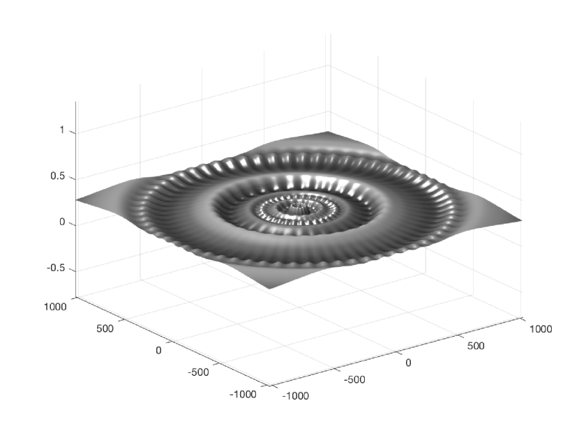
Figure 4.7. A plot of the scale-overlaps control function with $B/A\approx 1.54$, and the inner balls in the discretization of the corresponding frequency cover.

D.2. Representation of the frame operator

In the following, we denote by $\mathcal{L}$ the dual lattice of $\Lambda$; if $\Lambda=n^{-1}\mathbb{Z}^{d}$, with $n\in\mathbb{N}$, then $\mathcal{L}=n\mathbb{Z}^{d}$. We also use the notation: $\widehat{T}:=\mathcal{F}T\mathcal{F}^{-1}$, for the conjugation of an operator $T$ with the Fourier transform.

Lemma D.3 (Daubechies-like formula).

For $f\in H^{s}$:

(D.3) $${S_{\mathcal{F}}}f(\xi)=|\Lambda|^{-1}\sum_{\rho\in\mathcal{L}}S_{\rho}f(\xi),$$

where

(D.4) $$\widehat{S}_{\rho}\widehat{f}(\xi)=\sum_{j\geq 0}\sum_{k=1}^{n_{j}}2^{jd}\widehat{f}(\xi-2^{j}\rho)\overline{\widehat{\varphi}_{j,k}(\xi-2^{j}\rho)}\widehat{\varphi}_{j,k}(\xi).$$

Proof.

The representation follows from Poisson’s summation formula. See [13, Lemma 3.1] for related computations. ∎

Motivated by Lemma D.3, we introduced the following quantity. Let

(D.5) $$\Theta\left(\zeta\right)=\mathop{\mathrm{ess}\sup}_{\xi\in{\mathbb{R}^{d}}}\sum_{j\geq 0}\sum_{k=1}^{n_{j}}2^{jd}\left|\widehat{\varphi}_{j,k}^{sl}\left(\xi-2^{j}\zeta\right)\right|\left|\widehat{\varphi}_{j,k}^{sl}\left(\xi\right)\right|,\qquad\zeta\in{\mathbb{R}^{d}}.$$

Lemma D.4.

Let $s\in[0,1]$ and $S_{\rho}$, $\rho\in\mathcal{L}$ be given by (D.4), then

(D.6) $$\lVert S_{\rho}f\rVert_{H^{s}} \lesssim\max\left\{\Theta\left(\rho\right),\Theta\left(-\rho\right)\right\}\lVert f\rVert_{H^{s}}.$$

Proof.

Using (D.2) we estimate

$$(1+|\xi|)^{\alpha}\left|\widehat{S}_{\rho}\widehat{f}\left(\xi\right)\right| \leq\sum_{j,k}2^{jd}(1+|\xi-2^{j}\rho|)^{\alpha}\left|\widehat{f}\left(\xi-2^{j}\rho\right)\right|$$

$$\qquad(1+|\xi|)^{\alpha}\left|\widehat{\varphi}_{j,k}\left(\xi\right)\right|(1+|\xi-2^{j}\rho|)^{-\alpha}\left|\widehat{\varphi}_{j,k}\left(\xi-2^{j}\rho\right)\right|$$

(D.7) $$\lesssim\sum_{j,k}2^{jd}(1+|\xi-2^{j}\rho|)^{\alpha}\left|\widehat{f}\left(\xi-2^{j}\rho\right)\right|$$

$$\qquad(1+|\xi_{j,k}|)^{\alpha}\left|\widehat{\varphi^{sl}_{j,k}}\left(\xi\right)\right|(1+|\xi_{j,k}|)^{-\alpha}\left|\widehat{\varphi^{sl}_{j,k}}\left(\xi-2^{j}\rho\right)\right|$$

(D.8) $$=\sum_{j,k}2^{jd}(1+|\xi-2^{j}\rho|)^{\alpha}\left|\widehat{f}\left(\xi-2^{j}\rho\right)\right|\left|\widehat{\varphi^{sl}_{j,k}}\left(\xi\right)\right|\left|\widehat{\varphi^{sl}_{j,k}}\left(\xi-2^{j}\rho\right)\right|.$$

The conclusion now follows from Schur’s Lemma. ∎

Lemma D.5.

For a lattice $\Lambda$ with dual lattice $\mathcal{L}$ let

$$\Delta(\Lambda)=\sum_{\rho\in\mathcal{L}\backslash\left\{0\right\}}\max\left\{\Theta\left(\rho\right),\Theta\left(-\rho\right)\right\}.$$

Then there is constant $c>0$ such that, for $\Lambda=n^{-1}\mathbb{Z}^{d}$, $\Delta(\Lambda)\lesssim e^{-c\left|n\right|^{2}}$.

Proof.

Using Lemma D.1, we see that $\left|\Theta\left(\rho\right)\right|\lesssim e^{-c\left|\rho\right|^{2}}$, for some constant $c>0$, and the conclusion follows. See [13, Lemma 3.5] for a related argument. ∎

D.3. Proof of Theorem 2.1

We use the representation in Lemma D.3.

Step 1. Invertibility of the frame operator. Since ${S_{\mathcal{F}}}$ is self-adjoint on $L^{2}({\mathbb{R}^{d}})$, we only need to consider $s\in[0,1]$. Since

$$\widehat{S}_{0}\hat{f}(\xi)=\sum_{j\geq 0}\sum_{k=1}^{n_{j}}2^{jd}\left|\widehat{\varphi}_{j,k}(\xi)\right|^{2}\hat{f}(\xi),$$

it follows from Lemma D.1 that $S_{0}$ is invertible on $H^{s}$. We let $\Lambda=n^{-1}\mathbb{Z}^{d}$ with $n\in\mathbb{N}$. By Lemma D.3,

$$\lVert{S_{\mathcal{F}}}-S_{0}\rVert_{H^{s}\rightarrow H^{s}}\lesssim|\Lambda|^{-1}\Delta(\Lambda)\lesssim n^{d}e^{-cn^{2}}.$$

Therefore, we can choose $n$ such that ${S_{\mathcal{F}}}$ is invertible on $H^{s}$.

Step 2. Norm equivalence. For $s\in[-1,1]$, we use the Bessel bounds in Lemma B.5. These are stated only for the higher scales, but the extension the the zeroth-scale is straightforward. We conclude that

$$\lVert f\rVert_{H^{s}}^{2}\lesssim\lVert{S_{\mathcal{F}}}f\rVert_{H^{s}}^{2}\lesssim\sum_{\gamma\in\Gamma_{*}}4^{2sj}\left|\left<f,\varphi_{\gamma}\right>\right|^{2}\lesssim\lVert f\rVert_{H^{s}}^{2},$$

as claimed.

Appendix E Details on Figures 2.3 and 2.4

We considered the velocity $c(x_{1},x_{2})=2-0.4*\exp{(-(x_{1}^{2}+(x_{2}-5)^{2})/3)}$, $(x_{1},x_{2})\in\mathbb{R}^{2}$, and created a point source by summing $50$ frame elements with scale $j=4$, centered at the origin, and with frequency directions varying withing a 40-degree cone around the normal $(0,1)$. For convenience, the frame elements were constructed using as basic waveform the dilated Gaussian: $\exp(-2\pi\ln(16)(x_{1}^{2}+x_{2}^{2}))$ - cf. Figure 2.2. The GB evolution of the wavefront was computed from $t=0$ to $t=8.40$, following the construction described in Section 2.4. The ODEs have been solved with Matlab’s ODE45 routine. The wavefront goes through a caustic at time $t\approx 5.60$. A related example can be found in [3].

For longer times, the numerical solution to the Riccati equation becomes unstable. In the simulation, a tolerance of $\Im(M(t))>0.005$ was set, suppressing the beam if the condition was not satisfied. In order to improve the precision of the solution, one can reinitialize the algorithm by re-expanding the solution into wavepackets [52, 39, 46]. We expect that these techniques will lead to a full numerical implementation of the parametrix.

Appendix F Table of notation

Symbol	Description	Ref.
$\mathbb{R}^{d}_{+}$	$\mathbb{R}^{d}_{+}=(0,+\infty)\times\mathbb{R}^{d-1}$.	Sec. 1.5
$\mathbb{R}^{d}_{T}$	$\mathbb{R}^{d}_{T}=[-T,T]\times\mathbb{R}^{d-1}$.	Sec. 1.5
$x_{*}$	$x=(x_{1},x_{*})\in{\mathbb{R}^{d}}$, with $x_{1}\in\mathbb{R}$ and $x_{*}\in\mathbb{R}^{d-1}$	Sec. 1.5
$c=c(x)$	Velocity function.
$h=h(t,x_{*})$	Boundary data for the Dirichlet problem.	Sec. 4.1.1
$[C_{h,\mathrm{inf}},C_{h,\mathrm{sup}}]$	Temporal support of the boundary data.	Sec. 4.1.1
$C_{\mathrm{graz}}$	Constant related to the no-grazing ray assumption.	Sec. 4.1.1
$H^{\pm}=H^{\pm}(x,p)$	Signed Hamiltonian functions.	(2.18)
$H=H(x,p)$	Denotes generically either $H^{+}$ or $H^{-}$.
$\sigma(x,D)$	Kohn-Nirenberg quantization of a symbol $\sigma$	Sec. 1.5
$\xi_{j,k}$	Center for the frequency cover.	Sec. 2.1
$\tilde{\xi}_{j,k}$	Approximately normalized version of $\xi_{j,k}$.	(2.2)
$\Lambda$	A lattice within ${\mathbb{R}^{d}}$. Throughout most of the text, the choice of $\Lambda$ is fixed by Theorem 2.1
$\Gamma$	Basic scale-angle-position index set.	(2.4)
$\Gamma_{*}$	Superset of $\Gamma$ augmented with zero-scale.	(2.6)
$\Gamma_{0}$	A generic subset of $\Gamma$.
$\Gamma_{h}$	A subset of $\Gamma$ related to the frame expansion of $h$.	Sec. 4.2
$\Gamma_{h}^{\pm}$	Two subsets $\Gamma_{h}^{+}$ and $\Gamma_{h}^{-}$ that partition $\Gamma_{h}$.	(4.10)
$\gamma$	Generic element of (a subset of) $\Gamma_{*}$. We refer implicitly to the notation $\gamma=(j,k,\lambda)$.	Sec. 2.1
$\mathcal{S}=\mathcal{S}_{\gamma}$	A function that maps an index $\gamma$ into a tuple of initial conditions for a GB.	Sec. 2.4
$\mathcal{S}^{st}=\mathcal{S}^{st}_{\gamma}$	The standard choice for such a map.	Sec. 2.5
$\mathcal{S}^{h,\pm}=\mathcal{S}^{h,\pm}_{\gamma}$	Two particular maps defined on $\Gamma_{h}^{\pm}$ respectively, constructed in terms of the boundary value $h$.	Sec. 6
$\Phi^{\pm}_{\gamma}$	GB associated with $\gamma$ by means of an implicit map $\mathcal{S}_{\gamma}$.	Sec. 2.4
$\Phi_{\gamma}$	Denotes generically either $\Phi^{+}_{\gamma}$ or $\Phi^{+}_{\gamma}$.
$\Phi^{st,\pm}_{\gamma}$	The beams associated with $\mathcal{S}^{st}_{\gamma}$.	Sec. 2.5
$\Phi^{h,\pm}_{\gamma}$	The beam associated with $\mathcal{S}^{h,\pm}_{\gamma}$. Here the mode is determined by whether $\gamma\in\Gamma_{h}^{+}$ or $\Gamma_{h}^{-}$.	Sec. 6.1
$\varphi$	Normalized Gaussian function.	(2.3)
$\varphi_{\gamma}$	Frame element associated with $\gamma\in\Gamma_{*}$.	Sec. 2.1
$\phi_{\gamma}$	Generic wave molecule.	App. B
$\Upsilon$	Generic set of GB parameters, indexed by a corresponding function $\mathcal{S}$.	Rem. 2.4
$\Upsilon^{st}$	The standard choice for such a set.	Sec. 2.5
$\Upsilon^{h,\pm}$	Two particular such sets associated with $h$.	Sec. 6.1
$F={\mathbb{O}}^{m}(I,\Upsilon)$	A family of functions $F_{\gamma}$ that vanishes to oder $m$ on the centers of the beams defined by $\Upsilon$, uniformly on the time interval $I$.	Def. 3.3
$F=\mathbb{O}_{\geq}^{m}(I,\Upsilon)$	Functions with vanishing order at least $m$.	Def. 3.4

References

- [1] A. Aldroubi, C. Cabrelli, and U. M. Molter. Wavelets on irregular grids with arbitrary dilation matrices and frame atoms for . Appl. Comput. Harmon. Anal., 17(2):119–140, 2004.
- [2] F. Andersson, M. Carlsson, and L. Tenorio. On the representation of functions with Gaussian wave packets. J. Fourier Anal. Appl., 18(1):146–181, 2012.
- [3] F. Andersson, M. V. de Hoop, and H. Wendt. Multiscale discrete approximation of Fourier integral operators. Multiscale Model. Simul., 10(1):111–145, 2012.
- [4] F. Andersson, M. V. de Hoop, and H. Wendt. Multiscale reverse-time-migration-type imaging using the dyadic parabolic decomposition of phase space. SIAM J. on Imaging Sciences, 8(4):2383–2411, 2015.
- [5] V. M. Babich and V. S. Buldyrev. Asimptoticheskie metody v zadachakh difraktsii korotkikh voln. Tom l. Izdat. “Nauka”, Moscow, 1972. Metod ètalonnykh zadach. [The method of canonical problems], With the collaboration of M. M. Popov and I. A. Molotkov.
- [6] G. Bao, J. Qian, L. Ying, and H. Zhang. A convergent multiscale Gaussian-beam parametrix for the wave equation. Comm. Partial Differential Equations, 38(1):92–134, 2013.
- [7] N. Bleistein and S. H. Gray. Amplitude calculations for 3D Gaussian beam migration using complex-valued traveltimes. Inverse Problems, 26(8):085017, 28, 2010.
- [8] E. J. Candès and L. Demanet. The curvelet representation of wave propagators is optimally sparse. Comm. Pure Appl. Math., 58(11):1472–1528, 2005.
- [9] V. Červenỳ, M. M. Popov, and I. Pšenčík. Computation of wave fields in inhomogeneous media—gaussian beam approach. Geophysical Journal International, 70(1):109–128, 1982.
- [10] J. Chandra and P. W. Davis. Linear generalizations of Gronwall’s inequality. Proc. Amer. Math. Soc., 60:157–160 (1977), 1976.
- [11] A. Córdoba and C. Fefferman. Wave packets and Fourier integral operators. Comm. Partial Differential Equations, 3(11):979–1005, 1978.
- [12] I. Daubechies. The wavelet transform, time-frequency localization and signal analysis. IEEE Trans. Inform. Theory, 36(5):961–1005, 1990.
- [13] M. V. de Hoop, K. Gröchenig, and J. L. Romero. Exact and approximate expansions with pure Gaussian wave packets. SIAM J. Math. Anal., 46(3):2229–2253, 2014.
- [14] M. V. de Hoop, S. F. Holman, H. F. Smith, and G. Uhlmann. Regularity and multi-scale discretization of the solution construction of hyperbolic evolution equations with limited smoothness. Appl. Comput. Harmon. Anal., 33(3):330–353, 2012.
- [15] M. V. de Hoop, H. Smith, G. Uhlmann, and R. D. van der Hilst. Seismic imaging with the generalized Radon transform: a curvelet transform perspective. Inverse Problems, 25(2):025005, 21, 2009.
- [16] M. V. de Hoop, G. Uhlmann, A. Vasy, and H. Wendt. Multiscale discrete approximations of Fourier integral operators associated with canonical transformations and caustics. Multiscale Model. Simul., 11(2):566–585, 2013.
- [17] L. Demanet. Curvelets, wave atoms, and wave equations. PhD thesis, California Institute of Technology, 2006.
- [18] L. Demanet and L. Ying. Wave atoms and sparsity of oscillatory patterns. Appl. Comput. Harmon. Anal., 23(3):368–387, 2007.
- [19] L. Demanet and L. Ying. Wave atoms and time upscaling of wave equations. Numer. Math., 113(1):1–71, 2009.
- [20] G. A. Deschamps. Gaussian beam as a bundle of complex rays. Electronics Letters, 7(23):684–685, November 1971.
- [21] G. B. Folland. Harmonic analysis in phase space, volume 122 of Annals of Mathematics Studies. Princeton University Press, Princeton, NJ, 1989.
- [22] D.-A. Geba and D. Tataru. A phase space transform adapted to the wave equation. Comm. Partial Differential Equations, 32(7-9):1065–1101, 2007.
- [23] N. R. Hill. Gaussian beam migration. Geophysics, 55(11):1416–1428, 1990.
- [24] L. Hörmander. On the existence and the regularity of solutions of linear pseudo-differential equations. Secrétariat de l’Enseignement Mathématique, Université de Genève, Geneva, 1971. Série des Conférences de l’Union Mathématique Internationale, No. 1, Monographie No. 18 de l’Enseignement Mathématique.
- [25] A. Kachalov and M. Popov. Application of the method of summation of gaussian beams for calculation of high-frequency wave fields. In Soviet Physics Doklady, volume 26, page 604, 1981.
- [26] A. Katchalov, Y. Kurylev, and M. Lassas. Inverse boundary spectral problems, volume 123 of Chapman & Hall/CRC Monographs and Surveys in Pure and Applied Mathematics. Chapman & Hall/CRC, Boca Raton, FL, 2001.
- [27] J. B. Keller and W. Streifer. Complex rays with an application to gaussian beams. J. Opt. Soc. Am., 61(1):40–43, Jan 1971.
- [28] P. Kittipoom, G. Kutyniok, and W.-Q. Lim. Construction of compactly supported shearlet frames. Constr. Approx., 35(1):21–72, 2012.
- [29] H. Koch and D. Tataru. Dispersive estimates for principally normal pseudodifferential operators. Comm. Pure Appl. Math., 58(2):217–284, 2005.
- [30] A. Laptev and I. M. Sigal. Global Fourier integral operators and semiclassical asymptotics. Rev. Math. Phys., 12(5):749–766, 2000.
- [31] I. Lasiecka, J.-L. Lions, and R. Triggiani. Nonhomogeneous boundary value problems for second order hyperbolic operators. J. Math. Pures Appl. (9), 65(2):149–192, 1986.
- [32] J.-L. Lions and E. Magenes. Non-homogeneous boundary value problems and applications. Vol. I. Springer-Verlag, New York-Heidelberg, 1972. Translated from the French by P. Kenneth, Die Grundlehren der mathematischen Wissenschaften, Band 181.
- [33] H. Liu, O. Runborg, and N. M. Tanushev. Error estimates for Gaussian beam superpositions. Math. Comp., 82(282):919–952, 2013.
- [34] J. Lu and X. Yang. Frozen Gaussian approximation for high frequency wave propagation. Commun. Math. Sci., 9(3):663–683, 2011.
- [35] J. Lu and X. Yang. Convergence of frozen Gaussian approximation for high-frequency wave propagation. Comm. Pure Appl. Math., 65(6):759–789, 2012.
- [36] R. B. Melrose. Local Fourier-Airy integral operators. Duke Math. J., 42(4):583–604, 1975.
- [37] R. B. Melrose. Microlocal parametrices for diffractive boundary value problems. Duke Math. J., 42(4):605–635, 1975.
- [38] R. B. Melrose and M. Taylor. Boundary problems for wave equations with grazing and gliding rays. Manuscript, retrieved from: www.unc.edu/math/faculty/met/glide.pdf on 02/20/2017.
- [39] M. Motamed and O. Runborg. Taylor expansion and discretization errors in Gaussian beam superposition. Wave Motion, 47(7):421–439, 2010.
- [40] M. Nielsen. Frames for decomposition spaces generated by a single function. Collect. Math., 65(2):183–201, 2014.
- [41] L. Nirenberg. Lectures on linear partial differential equations. Uspehi Mat. Nauk, 30(4(184)):147–204, 1975. Translated from the English by Ju. V. Egorov (Amer. Math. Soc., Providence, R.I., 1973).
- [42] T. J. P. M. Op ’t Root, C. C. Stolk, and M. V. de Hoop. Linearized inverse scattering based on seismic reverse time migration. J. Math. Pures Appl. (9), 98(2):211–238, 2012.
- [43] M. M. Popov. A new method for calculating wave fields in high-frequency approximation. Zap. Nauchn. Sem. Leningrad. Otdel. Mat. Inst. Steklov. (LOMI), 104:195–216, 239–240, 1981. Mathematical questions in the theory of wave propagation, 11.
- [44] M. M. Popov. A new method of computation of wave fields using Gaussian beams. Wave Motion, 4(1):85–97, 1982.
- [45] J. Qian and L. Ying. Fast Gaussian wavepacket transforms and Gaussian beams for the Schrödinger equation. J. Comput. Phys., 229(20):7848–7873, 2010.
- [46] J. Qian and L. Ying. Fast multiscale Gaussian wavepacket transforms and multiscale Gaussian beams for the wave equation. Multiscale Model. Simul., 8(5):1803–1837, 2010.
- [47] J. Ralston. Gaussian beams and the propagation of singularities. In Studies in partial differential equations, volume 23 of MAA Stud. Math., pages 206–248. Math. Assoc. America, Washington, DC, 1982.
- [48] H. F. Smith. A Hardy space for Fourier integral operators. J. Geom. Anal., 8(4):629–653, 1998.
- [49] H. F. Smith. A parametrix construction for wave equations with coefficients. Ann. Inst. Fourier (Grenoble), 48(3):797–835, 1998.
- [50] C. C. Stolk. On the modeling and inversion of seismic data. Ph. D. thesis, Utrecht University, 2000.
- [51] C. C. Stolk. A pseudodifferential equation with damping for one-way wave propagation in inhomogeneous acoustic media. Wave Motion, 40(2):111 – 121, 2004.
- [52] N. M. Tanushev, B. Engquist, and R. Tsai. Gaussian beam decomposition of high frequency wave fields. J. Comput. Phys., 228(23):8856–8871, 2009.
- [53] D. Tataru. Phase space transforms and microlocal analysis. In Phase space analysis of partial differential equations. Vol. II, Pubbl. Cent. Ric. Mat. Ennio Giorgi, pages 505–524. Scuola Norm. Sup., Pisa, 2004.
- [54] A. Waters. A parametrix construction for the wave equation with low regularity coefficients using a frame of Gaussians. Commun. Math. Sci., 9(1):225–254, 2011.
- [55] V. H. Weston. Wave splitting and the reflection operator for the wave equation. In Inverse methods in action (Montpellier, 1989), Inverse Probl. Theoret. Imaging, pages 227–238. Springer, Berlin, 1990.