Scaling Active Search using Linear Similarity Functions
Abstract
Active Search has become an increasingly useful tool in information retrieval problems where the goal is to discover as many target elements as possible using only limited label queries. With the advent of big data, there is a growing emphasis on the scalability of such techniques to handle very large and very complex datasets.
In this paper, we consider the problem of Active Search where we are given a similarity function between data points. We look at an algorithm introduced by Wang et al. Wang et al. (2013) known as Active Search on Graphs and propose crucial modifications which allow it to scale significantly. Their approach selects points by minimizing an energy function over the graph induced by the similarity function on the data. Our modifications require the similarity function to be a dot-product between feature vectors of data points, equivalent to having a linear kernel for the adjacency matrix. With this, we are able to scale tremendously: for data points, the original algorithm runs in time per iteration while ours runs in only given -dimensional features.
We also describe a simple alternate approach using a weighted-neighbor predictor which also scales well. In our experiments, we show that our method is competitive with existing semi-supervised approaches. We also briefly discuss conditions under which our algorithm performs well.
1 Introduction
With rapid growth of the digital world, we are often faced with the task of quickly discovering and retrieving objects of interest from a large pool of data available to us. The task of finding specific pieces of information might require more sophisticated solutions than just key-word searches. Interactive approaches like Relevance Feedback can often be more effective, where an algorithm requests a user’s feedback on its results in order to improve. Active Search is an example of such an approach: it discovers targets by asking the user for information it considers useful. With user feedback, Active Search algorithms iteratively build a model of what constitutes relevant information. This carries two potential benefits in information retrieval problems: (1) these approaches need less labeled data and (2) they can focus on building a model of only the target class. The second point is useful for problems in which we are searching for the proverbial needle in a haystack. If there are relatively few targets, it is important to focus on modeling and identifying only those points. These approaches could be effective in real-world domains like product-recommendation and drug-discovery.
In this paper, we look at the problem of Active Search given a similarity function between data points. This function induces a graph over our data, with edge-weights as the similarities between points. We consider an existing approach of Active Search on Graphs by Wang et al. Wang et al. (2013) and make key modifications which allow us to scale substantially. While the original approach looks at purely graphical data, we consider data lying in a multi-dimensional feature space. The similarity function is taken to be some kernel over features vectors. The only requirement is it is finite dimensional with an explicit kernel space representation. In other words, the similarity function can explicitly be computed as the dot-product in this space.
The original algorithm requires pre-computation time, time per iteration and memory for data points. Ours only requires pre-computation time, time per iteration and memory for -dimensional feature vectors. While the original approach is not viable for datasets larger than around 20,000 points, our algorithm comfortably handles millions.
We also describe a simple approach using weighted neighbors which also scales to large datasets. This approach uses a Nadaraya-Watson-esque estimator to propagate labels, and runs in time for initialization and each iteration.
The contribution of this paper is the following: We present non-trivial modifications to an existing Active Search approach, scaling it multiple orders of magnitude. We describe a simple alternate which also scales well. We also touch upon when our algorithm will perform well.
This paper is structured as follows. We describe the existing literature in Section 2. We formally state the problem of Active Search in Section 3. In Section 4, we describe the existing approach followed by our modifications. In Section 5, we discuss conditions for good performance. We describe our experiments and discuss results in Section 6. We conclude in Section 7, and mention related challenges and next steps.
2 Related Work
Over the past few years, there has been significant research done in semi-supervised active learning. Most of this research is driven towards learning good classifiers given a limited labeled data, as opposed to recovering target points.
Guillory et al. Guillory and Bilmes (2009) propose methods for selecting labeled vertex sets on a graph in order to predict the labels of other points. Cesa-Bianchi et al. Cesa-Bianchi et al. (2013) explore an active version of this where they consider the optimal placement of queries on a graph to make minimal mistakes on the unlabeled points.
Zhu et al. Zhu et al. (2003a) propose a method to perform semi-supervised learning on graphs. They formulate their problem in terms of a Gaussian random field on the graph, and efficiently compute the mean of the field which is characterized by a harmonic function. They extend this in Zhu et al. (2003b) to make it active: given the above graphical construction, they query points using a greedy selection scheme to minimize expected classification error. Zhu et al. Zhu and Lafferty (2005) describe a scalable method to perform inductive learning using harmonic mixtures, while preserving the benefits of graph-based semi-supervised learning.
There has also been some work on optimization-based approaches for semi-supervised classification. Melacci et al. Melacci and Belkin (2011) propose a method they call LapSVM, which builds an SVM classifier using the graphical structure of the data. Zhang et al. Zhang et al. (2009) describe the Prototype Vector Machine which solves a similar objective as above, by approximating it using “prototype” vectors which are representative points in the data. Liu et al. Liu et al. (2010) introduce an approach which also considers representative samples from the data called Anchors. They construct an “Anchor Graph”, and make predictions in the main graph based on weighted combinations of predictions on Anchors.
Ma et al. Ma et al. (2015) describe new algorithms which are related to the multi-armed bandit problem to perform Active Search on graphs. Their algorithms are based on the -optimality selection criterion, which queries the point that minimizes the sum of the elements in the predictive covariance as described in Ma et al. (2013). Kushnir Kushnir (2014) also incorporate exploration vs. exploitation in their work on active transductive learning on graphs. They do this by considering random walks on a modified graph which combines the data distribution with their label hypothesis, allowing them to naturally switch from exploring to refinement.
There have also been Active Search approaches which focus on recall instead of classification. Garnett et al. Garnett et al. (2012) perform Active Search and Active Surveying using Bayesian Decision theory. Active Surveying seeks to query points to predict the prevalence of a given class.
Closely related to our work is that of Wang et al. Wang et al. (2013) where they perform Active Search on graphs. They select points by minimizing an energy function over the graph. They also emulate one-step look-ahead by a score reflecting the impact of labeling a point. Our work extends this with crucial modifications allowing us to scale to much larger data sets.
3 Problem Statement
We are given a finite set of points , and their unknown labels where . We are also given a similarity function between points. We consider the case where this function is linear over some explicit feature transformation : . This is analogous to the explicit kernel-space representation of some finite-dimensional kernel. This induces a graph over the data: the edge weight between and is given by .
Initially, we are given a small set of labeled points , while the remaining points are in the unlabeled set, . Every iteration, we query one point in for its label and move it to the labeled set . The goal is to find as many positive points as possible after iterations, where is a fixed budget for labeling points.
4 Approach
4.1 Background: Active Search on Graphs [ASG]
We briefly describe the algorithm introduced by Wang et al. Wang et al. (2013). They interpret the data as a graph where the edge-weights between points is given by the similarity . Their method then uses a harmonic function to estimate the label of data points, inspired by the work done by Zhu et al. Zhu et al. (2003a). This is done by minimizing the energy:
| (1) |
The function serves as the primary measure for querying a point to label. If is positive and semi-definite, the optimal solution can be interpreted intuitively through random walks on the graph: is the probability that a random walk starting at the point reaches a positively labeled point before a negatively labeled point. The following is a brief explanation: Here, for simplicity, we take to be the vector where . Setting the gradient of the energy to 0, we get at optimum where and are the adjacency and diagonal degree matrices respectively. The rows of are exactly the transition probabilities from each node on the graph, and thus, the entire matrix can be interpreted as the transition matrix of the random walk. The interpretation of directly follows from this.
Wang et al. then describe a problem they call hub-blocking, where a negatively labeled point is the center of a hub structure connected to multiple positive but unlabeled points. Discovering another positive elsewhere in the graph will not help discover the positive unlabeled nodes in the hub, as they are blocked off by the negatively labeled hub center. To overcome this, they propose a soft-label model: every labeled point is now connected to a pseudo-node which holds the label instead. A random walk now terminates only when reaching the pseudo-node of a labeled point. A similar augmentation incorporates prior probabilities: a pseudo-node is attached to every unlabeled point and holds the prior probability of being positive. The transition probability from a point to its psuedo-node is constant across labeled or unlabeled points.
The following is the resulting energy function over :
| (2) |
where , , and the regularizing constants and depend on transition probabilities into pseudo-nodes. Explicitly, if and are transition probabilities into labeled and unlabeled pseudo-nodes respectively, then and . The minimizer of the energy function can be solved by setting the gradient to 0. We assume, without loss of generality, that the labeled and unlabeled indices are grouped together. The minimizer is111Derived in the Appendix.:
| (3) |
This solution can also be obtained by performing label propagation in the augmented graph. For simplicity of notation, will simply be denoted by moving forward.
To pick points for label queries, ASG uses a heuristic called the Impact Factor which looks at the change of values if a given unlabeled point was labeled as positive.
The final selection criterion is . With this, ASG iteratively queries labels and updates and . ASG has an time initialization and time per-iteration.
4.2 Linearized Active Search [LAS]
Here, we describe our algorithm. We now require feature vectors for our points. The similarity function is then assumed to be be linear in these features (or some explicit transformation of them). This requirement is often not too restrictive; in fact, some popular kernels can be approximated using a linear embedding into some feature space. For example, the RBF kernel can be approximated by Random Fourier Features Rahimi and Recht (2007). For simplicity, let itself represent the feature vector. The similarity between two points is then .
Here is the algorithm at a glance. At a high level, LAS is the same as ASG:
-
•
Initialization: Initialize with starting label set . Pre-compute relevant quantities which can be updated.
-
•
In each iteration: Request the next label with a selection criterion based on and . Update all relevant quantities given this label.
Note: As mentioned before, ASG requires purely graphical data as input, i.e. the graph adjacency matrix. LAS works with a different class of data, which lives in some multi-dimensional feature space. A graph is induced over the data by the similarity function. If the input to ASG and LAS is the same, the results will be identical. By “the same”, we mean the adjacency matrix for ASG is the same as the one of the induced graph for LAS. In this case, and the point queried will be identical at every iteration.
The pseudo-code is given in Algorithm 1. We now discuss how a linear similarity function helps us update efficiently.
4.2.1 Initialization
The adjacency matrix is where , with points and features. Then, . This gives us:
Using the matrix inversion lemma, we get222Derived in the Appendix.:
| (4) |
| (5) |
This converts an time matrix inverse in ASG into the time inverse of . For large datasets, we can expect . Below, we show that we only need to invert once; its inverse can be efficiently updated every iteration.
The initialization runs in time for computing and for computing . Next, we describe our efficient updates to and given a new label.
4.2.2 Updates to on receiving a new label
We have at the previous iteration. Only one element in changes each iteration. Take superscript + to mean the updated value of a variable. We have:
where and is the standard basis vector. Using the matrix inversion lemma:
| (6) |
Only one element in changes: . Thus, the update to can be calculated as333Updates derived in the Appendix.:
This takes time per-iteration as it just involves cascading matrix-vector multiplications.
4.2.3 Impact Factor
LAS also includes appropriate modifications for the initialization and updates of the Impact Factor which adhere to the improved running time. We do not describe these here as they are much more involved than those above, while not being fundamentally complicated.444Derived in the Appendix. We also slightly changed the Impact Factor from ASG: we scaled so that it has the same mean as the vector. This allows us to tune without worrying about the magnitude of values in , which varies based on the dataset.
4.3 Weighted Neighbor Active Search [WNAS]
Here, we briefly describe a simple and intuitive alternate approach for query selection which also scales well with large amounts of data. This approach is similar to the Nadaraya-Watson kernel regressor:
The updates for for this approach are simple. We keep track of the numerator and denominator individually for each unlabeled point. Each time we get a new labeled point , we can compute its similarity to all other unlabeled points efficiently as the following vector:
We can then update the numerator and denominator of all unlabeled points directly from this vector. The numerators would be updated by adding and the denominators would be updated by adding . These computations require time for initialization and iteration.
5 Analysis of Active Search
5.1 Good Similarity Functions for Active Search
How do we know if our similarity function is “good” for our problem, i.e., under what conditions will it give us a high recall rate for a given dataset? Not all similarity functions are suited to a given problem, even if they provide non-trivial information. For example, consider a similarity function which, given two animals, outputs 1 if they share the same number of legs and 0 otherwise. This similarity function will be useful to distinguish human beings from cats but not cats from dogs. But the similarity function itself is not useless.
Assume that the similarity function only takes non-negative values. This allows us to interpret them as unnormalized probabilities. can be written as555Derived in the Appendix.:
Let: . Given , we get:
M has the same sparsity structure as A, as all its off-diagonal elements are the negative of those in A. Since is a diagonally dominant symmetric matrix with non-positive off-diagonal entries, it is a Stieltjes matrix. This means that its inverse is symmetric and non-negative. Grouping indices by their class without loss of generality, we have as
This gives us:
| (7) |
where and are indicator vectors of whether the points are labeled or not, for the positive and negative points respectively. We only need to look at labeled points since for any unlabeled point , . Here, can be interpreted as a parameter instead of the constant prior, measuring “importance” of labels: if is low, then we consider each received positive label as very informative and vice-versa.
Equation 7 says that if the elements in are small, then will better reflect the labels of points. But when are these off-diagonal elements small? We can show that if the cross-class similarities, or off-diagonal blocks of A, are low in a matrix-norm sense, then the same is true in :
Lemma 5.1
Let where is the block diagonal component of the similarity matrix and is the pure cross-similarity component.
If , then where and is the minimum degree in the graph.666Proved in the Appendix.
Intuitively, a bound on bounds the between-class similarity. Lemma 5.1 then tells us that if our similarity respects the underlying label distribution, then the computed will do the same. This only gives us information within a given iteration of Active Search; it does not directly give bounds on errors when querying the highest node in every iteration. But it is a step towards understanding the relationship between the similarity function and the performance.
5.2 Comparison of ASG/LAS and WNAS
ASG (or equivalently LAS) and WNAS often have similar performance on recalling positive points. This is because, locally around the labeled points, both approaches propagate labels in a similar manner. The label confidences assigned by WNAS can also be interpreted as one step of a random-walk as follows. For each unlabeled point, consider the graph containing it, along with all labeled points. Its score is equivalent to the probability that a random walk starting from that point transitions into a positive in one step.
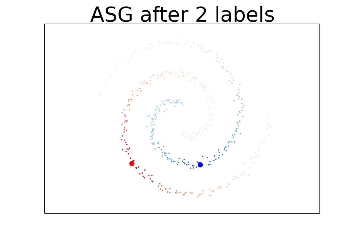
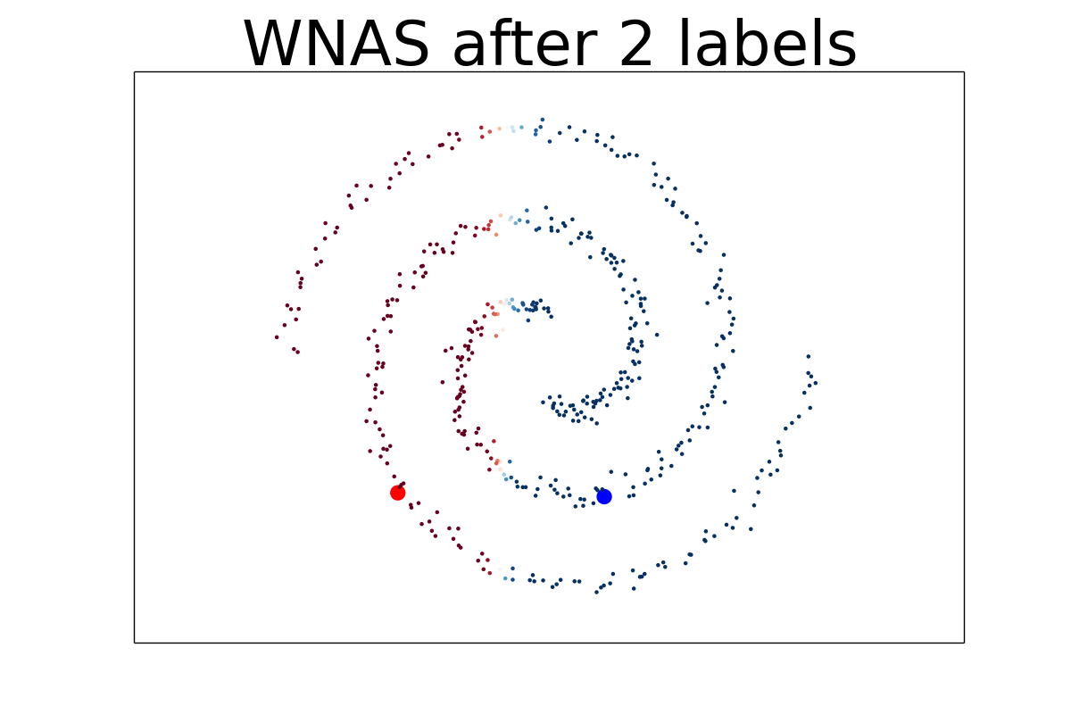
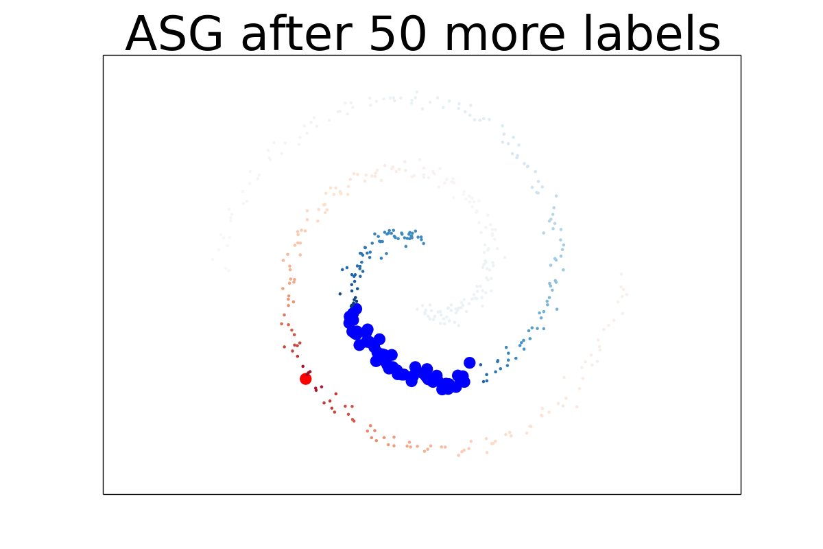
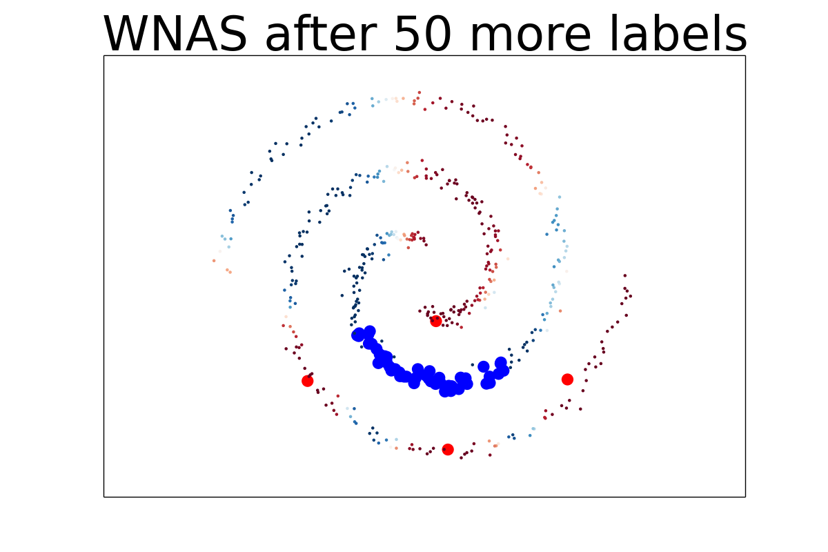
However, while WNAS makes use of local structure of the graph around the labeled points, it does not effectively use the global connectivity structure of the graph. The relevance of this can be seen in the swiss-roll dataset in Figure 1; where the inner blue roll is positive and the outer red roll is negative. The predictions of WNAS and ASG are similar around the labeled points, but very different away from them. The usefulness of WNAS’ score diminishes rapidly moving away from the label set, unlike for ASG.
Another note is that computing an equivalent Impact Factor for WNAS requires computation, since we need to compute the similarity between every pair of unlabeled points. This makes the Impact Factor computation infeasible for large datasets, unlike LAS as discussed before.
| CoverType | MNIST | Adult | ||||
|---|---|---|---|---|---|---|
| 250 | 500 | 200 | 400 | 100 | 200 | |
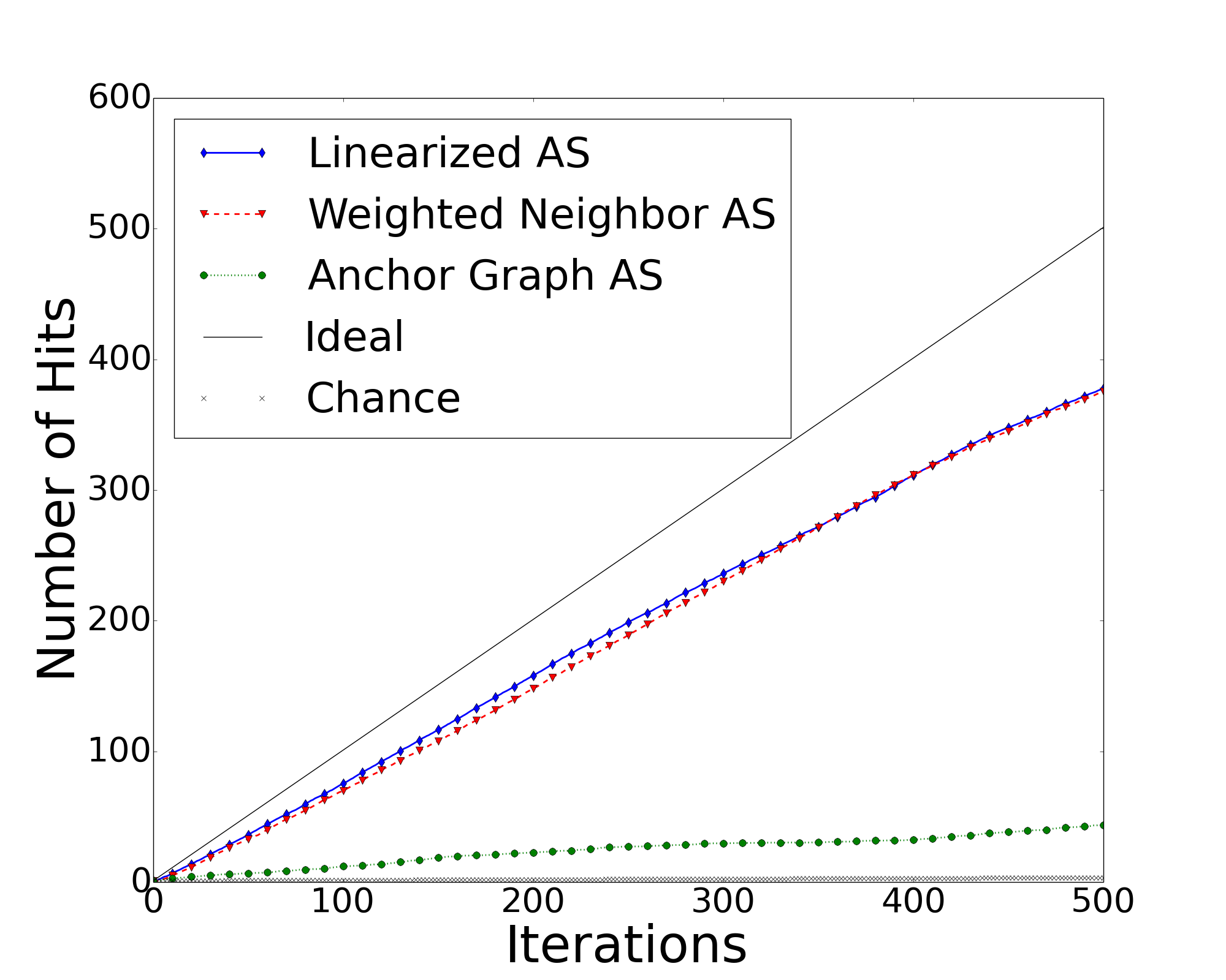
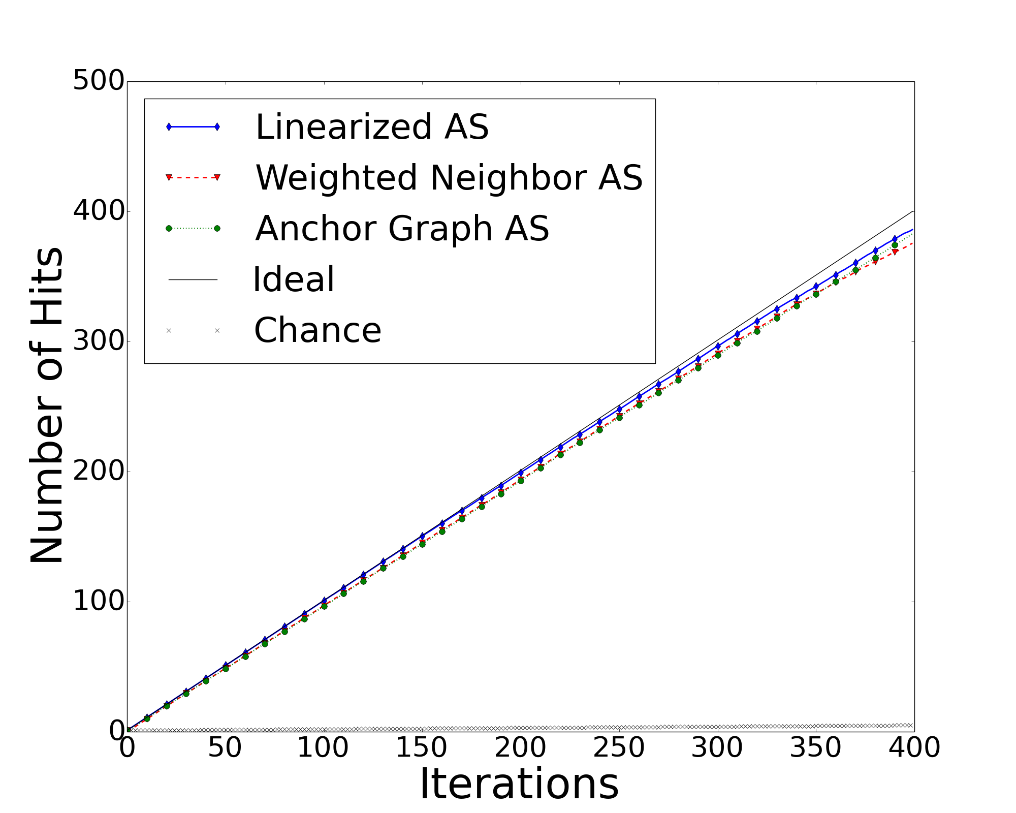
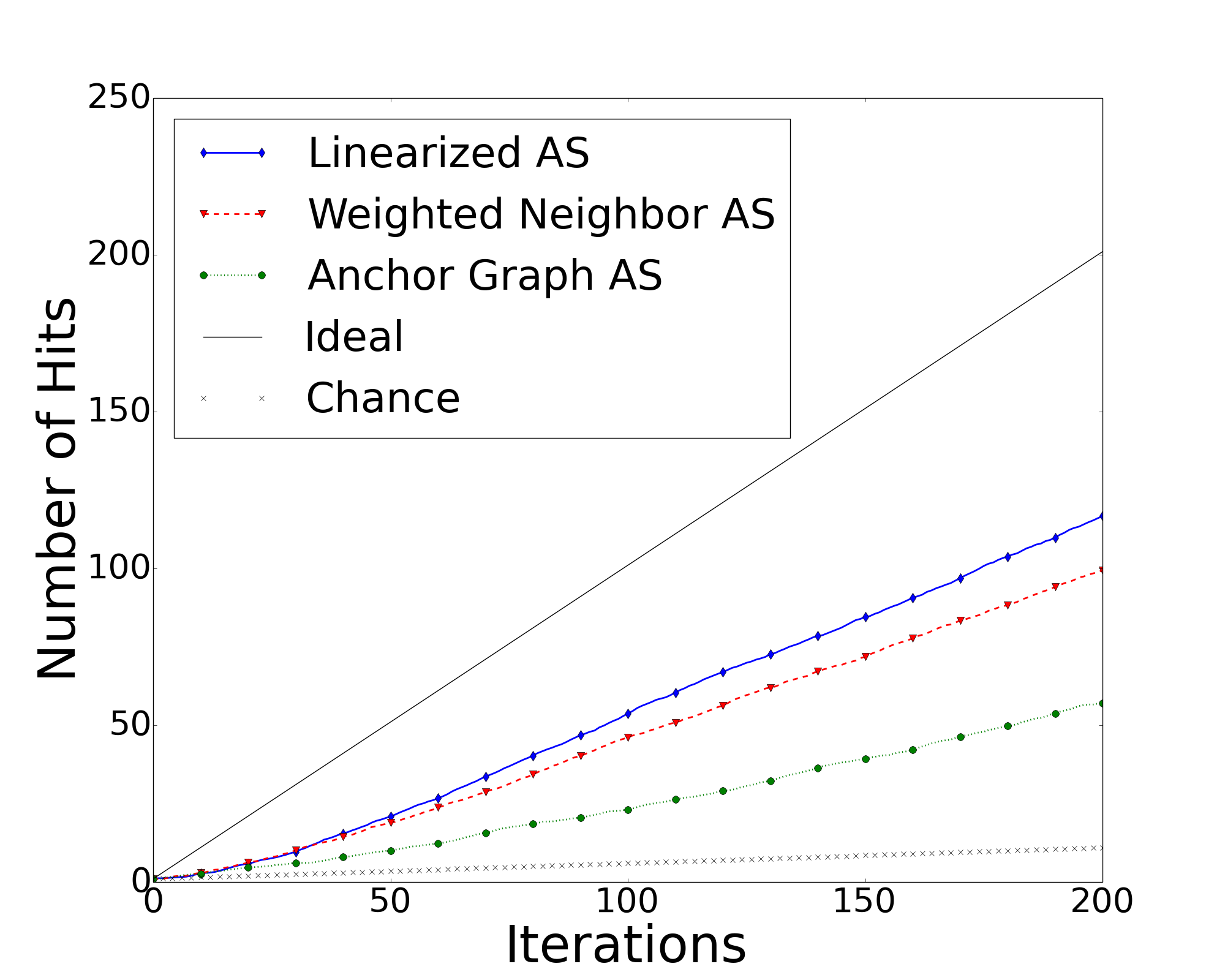
| LAS | 198.7 32.0 | 377.8 55.7 | 199.5 1.0 | 386.4 4.9 | 53.7 11.7 | 116.7 13.3 |
| WNAS | 188.8 21.5 | 375.7 37.9 | 193.7 3.0 | 379.8 7.2 | 46.1 16.3 | 99.4 26.4 |
| AGR | 27.2 11.2 | 43.5 11.8 | 192.8 3.1 | 380.1 4.0 | 23.1 18.5 | 57.1 39.2 |
6 Experiments
We performed experiments on the following datasets: the CoverType and Adult datasets from the UCI Machine Learning Repository and MNIST.
The Covertype dataset contains multi-class data for different forest cover types. There are around 581,000 points with 54-dimensional features. We take the class with the lowest prevalence of as positive. The data is unit normalized across features and a bias feature is appended to give 55 in total. Then, we project these onto a 550-dimensional space using Random Fourier Features Rahimi and Recht (2007) to approximate an RBF Kernel.
The Adult dataset consists of census data with the task of predicting whether a person makes over $50k a year or not. It contains 14 features which are categorical or continuous. The continuous features are made categorical by discretization. Each feature is converted into a one-hot representation with binary features for categories. The features are then unit normalized. The positives are those making more than $50k a year. We modified the dataset size to make the target prevalence 5%. The final dataset has a 39,000 points.
For the MNIST dataset, we combine the training, validation and testing sets into one. The 28x28 pixel images give us 784 features which are then unit normalized. We take the positive class to be the digit 1, and modified its prevalence to be 1%. The final dataset has around 63,500 points.
We compare LAS and WNAS to Anchor Graph Regularization with Local Anchor Embedding [AGR] as described in Liu et al. (2010)777This was re-implemented in Python for our experiments.. Their approach creates a proxy graph called the Anchor Graph which approximates the larger dataset; the labels given to points are then a weighted combination of the labels of the anchor points. Since this is a semi-supervised classification approach, we retrain it every iteration with all the data and known labels. We then use the confidence values for each unlabeled point to be positive as the value. This algorithm requires anchors to be computed beforehand. For this, we generated k-means over the transformed data points, with for each dataset.
Our main experiment measured recall (number of positives found) over a fixed number of iterations for each dataset. For each dataset, 10 runs were performed starting with one randomly chosen positive as initialization. For LAS, we took (the coefficient for the Impact Factor) to be the best from empirical evaluations. This was for CoverType and Adult, and 0 for MNIST. was taken as the true positives prevalence.
We also carried out smaller experiments over each dataset where we studied the predictive performance of LAS vs. WNAS immediately after initialization. Here, we randomly sampled 100 pairs of one positive and one negative point to initialize. Then, we reported the number of positives in the top 100 unlabeled points according to their -values. These 100 pairs did not include “bad” initializations, where neither approach found any positives.
Note: We did not compare our approach vs. purely graph based methods as in the Wang et al. (2013) Since our results are identical to ASG given the “same” data as described before, we only considered data with feature vectors.
6.1 Results
Figure 2 shows plots of the recall per iteration of LAS, WNAS and AGR for the different datasets. Table 1 shows mean recall and standard deviation of these experiments in the mid and final iteration. LAS and WNAS both have good performance in all three experiments. The CoverType dataset has high variance in estimates, likely because the data has many scattered positives which are not very informative during initialization. The algorithms would then take longer to discover the remaining positives. The MNIST data-set showed particularly good performance across the different approaches; all three approaches have near ideal recall. This is likely because the targets are tightly clustered together in the feature-space. The performance of AGR in the CoverType, though much better than random choice, is poorer than the other approaches. This is because AGR incurs significant overhead in the initialization of the algorithm. Computing k-means, followed by the weights and the reduced Laplacian of the Anchor Graph takes a few hours for CoverType. Furthermore, any change in the feature function used between the data points requires recomputation of the Anchor Graph. Due to this, we only used 500 Anchors even though it is a larger data-set. This poorer approximation of the data likely led to worse performance.
Table 2 shows the comparison between LAS and WNAS given a single positive and negative point for initialization. As expected from our discussion in Section 5.2, LAS generalizes better with the unlabeled data.
Note: We also conducted similar experiments on much larger datasets from the UCI Repository: the HIGGS dataset (5.5 million points) and the SUSY dataset (2.5 million points). We have not reported these results. These experiments were not any more informative than those above; they just served as a demonstration of scale.
| Dataset (pos%) | LAS | WNAS |
|---|---|---|
| Covertype (0.47%) | 4.19 | 1.66 |
| MNIST (1.00%) | 94.25 | 60.68 |
| Adult (5.00%) | 27.25 | 17.29 |
7 Conclusion and Future Work
In this paper, we proposed an algorithm to perform Active Search given a linear similarity function between data points. Through experiments, we demonstrate the scalability of our algorithm as compared to the original approach by Wang et al. (2013), as well as good recall on different datasets.
We also described an alternate, simple approach using a weighted neighbor estimator of labels. This approach also scales well to large datasets, but is not as generalizable given very little labeled information. It does perform comparably with our main approach in the recall problem.
7.1 Future Work
We require a “good” similarity function, or equivalently a good featurization, for our approach to perform well. A next step would be to learn a featurization simultaneously while performing Active Search. The challenge here is effective regularization with very little labeled data at the beginning.
We have also not dealt with natural graphs in this paper, because of the restriction on our similarity function. But we know that every iteration of Active Search just uses label propagation to compute . There exist methods, such as Fujiwara and Irie (2014), to perform efficient label propagation on large sparse graphs. Incorporating this into our approach along with appropriate Impact Factor computation would allow us to scale on natural graph datasets.
Acknowledgments
Work partially supported by DARPA (FA8750-12-2-0324, FA8750-14-2-0244) and NSF (1320347).
References
- Cesa-Bianchi et al. [2013] Nicolo Cesa-Bianchi, Claudio Gentile, Fabio Vitale, and Giovanni Zappella. Active learning on trees and graphs. arXiv preprint arXiv:1301.5112, 2013.
- Fujiwara and Irie [2014] Yasuhiro Fujiwara and Go Irie. Efficient label propagation. In Proceedings of the 31st international conference on machine learning (ICML-14), pages 784–792, 2014.
- Garnett et al. [2012] Roman Garnett, Yamuna Krishnamurthy, Xuehan Xiong, Jeff Schneider, and Richard Mann. Bayesian optimal active search and surveying. arXiv preprint arXiv:1206.6406, 2012.
- Guillory and Bilmes [2009] Andrew Guillory and Jeff A Bilmes. Label selection on graphs. In Advances in Neural Information Processing Systems, 2009.
- Kushnir [2014] Dan Kushnir. Active-transductive learning with label-adapted kernels. In Proceedings of the 20th ACM SIGKDD international conference on Knowledge discovery and data mining, pages 462–471. ACM, 2014.
- Liu et al. [2010] Wei Liu, Junfeng He, and Shih-Fu Chang. Large graph construction for scalable semi-supervised learning. In Proceedings of the 27th international conference on machine learning (ICML-10), pages 679–686, 2010.
- Ma et al. [2013] Yifei Ma, Roman Garnett, and Jeff Schneider. -optimality for active learning on gaussian random fields. In Advances in Neural Information Processing Systems, 2013.
- Ma et al. [2015] Yifei Ma, Tzu-Kuo Huang, and Jeff Schneider. Active search and bandits on graphs using sigma-optimality. 2015.
- Melacci and Belkin [2011] Stefano Melacci and Mikhail Belkin. Laplacian Support Vector Machines Trained in the Primal. Journal of Machine Learning Research, 12:1149–1184, March 2011.
- Rahimi and Recht [2007] Ali Rahimi and Benjamin Recht. Random features for large-scale kernel machines. In Advances in neural information processing systems, pages 1177–1184, 2007.
- Wang et al. [2013] Xuezhi Wang, Roman Garnett, and Jeff Schneider. Active search on graphs. In Proceedings of the 19th ACM SIGKDD International Conference on Knowledge Discovery and Data Mining, KDD ’13, 2013.
- Zhang et al. [2009] Kai Zhang, James T Kwok, and Bahram Parvin. Prototype vector machine for large scale semi-supervised learning. In Proceedings of the 26th Annual International Conference on Machine Learning, pages 1233–1240. ACM, 2009.
- Zhu and Lafferty [2005] Xiaojin Zhu and John Lafferty. Harmonic mixtures: combining mixture models and graph-based methods for inductive and scalable semi-supervised learning. In Proceedings of the 22nd international conference on Machine learning. ACM, 2005.
- Zhu et al. [2003a] Xiaojin Zhu, Zoubin Ghahramani, John Lafferty, et al. Semi-supervised learning using gaussian fields and harmonic functions. In ICML, 2003.
- Zhu et al. [2003b] Xiaojin Zhu, John Lafferty, and Zoubin Ghahramani. Combining active learning and semi-supervised learning using gaussian fields and harmonic functions. In ICML 2003 workshop on the continuum from labeled to unlabeled data in machine learning and data mining, 2003.
Appendix A Algorithm Derivations
A.1 Derivation of minimizer of E()
We can rewrite the energy function using matrices as given below. The subscripts and represents portions of various quantities as belonging to the set of labeled and unlabeled points respectively. Here, without loss of generality, we have rearranged the -vector to group the labeled and unlabeled points. This re-arrangement will hold throughout this appendix.
where
Let . Then, .
Notice that the energy function is convex in , since the Hessian is diagonally dominant and symmetric. The gradient of the above expression w.r.t. is:
where . Setting this to 0, we get the global minimizer:
The last line can be readily verified given
A.2 Derivation of Initialization step
We have that . The Kailath variant of the matrix inverse lemma gives:
Using this, we have:
A.3 Derivation of Updates
We have from last iteration. Further, only one element in changes:
, where . Expanding , we get:
Here, we use Woodbury’s Matrix inversion formula:
From this, we have:
Given that only one element in changes each iteration: , our updated becomes
Each step in this process only involves operations. Thus, this is the overall run-time per iteration.
A.4 Representation of
Here, we show how we can write as:
where
,
and is, as before, the vector with true labels for labeled points and otherwise.
From the derivation for the initialization, we can rearrange the terms and move some constants around as follows:
A.5 Derivation of Impact factor
The impact factor is defined to be the following:
where is the new score for after is labeled by the user. It is the change in over all unlabeled points, conditioned on the labeling as positive. Here is a brief description of this computation, followed by the detailed derivation.
In order to compute this, we look at the change in given a positive label.
We write as shown in A.4. We can now reason about the change vector of given that unlabeled point is a positive:
The following quantities can be computed directly from these change vectors.
The element of the above vectors is computed assuming that has a positive label. But, we still take to be in for the computation of because it simplifies computation, and can be corrected for. Further, only unlabeled entries matter in the computation, since the Impact Factor only depends on .
The Impact Factor can be written as follows, where denotes the element-wise product:
| (8) |
We subtract to correct for including in in previous computations.
We can shown that each term, and hence the whole Impact Factor, can be computed in time per iteration.
The detailed steps follow below.
From A.4, we have that . With this, we can write two equations:
where . If we label point as positive, subtracting the second equation from the first, we get:
with the standard basis vector . The last equality is true for the following reasons. Since we labeled point , we have and and for all , . Secondly, is 0 for every entry other than the diagonal entry, since only that element changes in . This tells us that when we label point , we have:
Substituting for the Impact Factor and using the notation , we get:
| (9) |
Using this, we can compute the two quantities of interest we defined before:
Let where the label of is taken as 1.
As mentioned before, is still included in .
Computing : In equation 9, we first solve for and subtract out . This gives us the element of as:
| (10) |
Computing : Notice that where is the indicator vector where if is unlabeled and 0 otherwise. Using since is symmetric, equation 9 gives us:
| (11) |
Now, note that , since this denotes after is labeled. And, since is unlabeled at the start of this iteration. and do not depend on the label itself, just on whether is labeled or not. With this, we can define new vectors which are the stacked versions of and :
These vectors only are relevant in the indices of the unlabeled points. Now, stacking equation 11 for all , we get:
| (12) |
If we are able to compute , and efficiently, then can be computed efficiently as it is just a constant number of point-wise operations. Further, the Impact is also readily computed as:
| (13) |
As noted before, we need to account for considering not removing from while computing each component of . Thus, we have to subtract before computing the final Impact Factor.
In the following sections, we will discuss how to compute , and efficiently.
A.5.1 Rewriting
The last step comes from the fact that . For our problem, . Using the same steps as in Section A.2:
| (14) |
where and . The individual matrices in the above expression are already being computed in updates for .
A.5.2 Computing given
We have
Given , we can compute in time as it consists of only element-wise sums and multiplications. Further, can be computed as follows.
-
•
changes only one element each iteration. It can be initialized once and can be updated.
-
•
can then be computed in time by cascading the matrix-vector multiplication in.
These operations take time per iteration.
A.5.3 Computing via updates
We have
where each element is given by equation 10. This can be written as:
| (15) |
where . We compute as follows:
Thus,
| (16) |
From this, we see that we just need to store and update every iteration. Here’s how we can do this:
-
•
We initialize and at the start. This computation takes time once we have .
-
•
Then, as we update , we also update . Here, is the index of the point to be labeled and is the index of being modified.
Therefore,
where is already computed in the updates to . Since is also computed while updating , updating each element only takes time because it consists of only a dot product and a constant number of scalar operations.
Thus, updating the entire vector only takes per iteration. Once we have , we can compute in time through element-wise operations.
Finally, after computing , we can compute in time every iteration, again using only element-wise sums and products.
A.5.4 Putting it all together
We showed that in computing both and , we need only initialization time and time per iteration of the algorithm. Then, putting them together to get the Impact Factor takes only time. This is the same as what is needed to compute the initialization and updates for .
In this way, the Impact Factor computation also scales with the other computations performed in the algorithm.
Appendix B Proofs
B.1 Proof of Lemma 4.1
The adjacency matrix is assumed to only have positive values.
Lemma 4.1
Let where is the block diagonal component of the similarity matrix and is the pure cross-similarity component.
If , then
where and is the minimum degree in the graph.
Proof: We want to show that if is “close” to block diagonal, then is close to block diagonal. We have that:
where is block diagonal. Using Woodbury’s Matrix Inversion lemma, we have:
Thus, where we have that is block diagonal. Taking the 1-norm of this, we have from sub-multiplicity of induced matrix norms:
Here, we use a result by Varah varah which is as follows:
For a diagonal dominant matrix ,
where , is the diagonal dominance defined by
For , we have as the contribution of to is 0. The minimum value of is then lower bounded by . Further, since only introduces off diagonal elements to , we have that for all . Thus, the minimum value for is also lower bounded by . This means that:
Since and are symmetric, we have that
as the 1-norm is the maximum absolute row-sum and the -norm is the maximum absolute column sum.
This finally gives us:
If we write where is the block diagonal component of and is the off block diagonal component, we have that:
Further, we have that since we are just introducing numbers where is 0. This can only increase the absolute row-sums. With this, we have that
Since is the block diagonal component of , it is exactly the following as defined in Section 5.1:
This gives us that
References
- [1] Varah, James M A lower bound for the smallest singular value of a matrix 1975.