Transformations between nonlocal and local integrable equations
Abstract
Recently, a number of nonlocal integrable equations, such as the -symmetric nonlinear Schrödinger (NLS) equation and -symmetric Davey-Stewartson equations, were proposed and studied. Here we show that many of such nonlocal integrable equations can be converted to local integrable equations through simple variable transformations. Examples include these nonlocal NLS and Davey-Stewartson equations, a nonlocal derivative NLS equation, the reverse space-time complex modified Korteweg-de Vries (CMKdV) equation, and many others. These transformations not only establish immediately the integrability of these nonlocal equations, but also allow us to construct their analytical solutions from solutions of the local equations. These transformations can also be used to derive new nonlocal integrable equations. As applications of these transformations, we use them to derive rogue wave solutions for the partially -symmetric Davey-Stewartson equations and the nonlocal derivative NLS equation. In addition, we use them to derive multi-soliton and quasi-periodic solutions in the reverse space-time CMKdV equation. Furthermore, we use them to construct many new nonlocal integrable equations such as nonlocal short pulse equations, nonlocal nonlinear diffusion equations, and nonlocal Sasa-Satsuma equations.
I Introduction
The study of integrable nonlinear wave equations has a long history Ablowitz1981 ; Zakharov1984 ; Faddeev1987 ; Ablowitz1991 ; Yang2010 . Most of those integrable equations are local equations, i.e., the solution’s evolution depends only on the local solution value and its local space and time derivatives. The Korteweg-de Vries equation and the nonlinear Schrödinger (NLS) equation are such examples.
Recently, a number of new nonlocal integrable equations were proposed and studied AblowitzMussPRL2013 ; AblowitzMussPRE2014 ; Yan ; Khara2015 ; AblowitzMussNonli2016 ; Zhu1 ; Fokas2016 ; Lou ; Lou2 ; AblowitzMussSAPM ; Chow ; ZhoudNLS ; ZhouDS ; HePTDS ; HePPTDS ; Zhu2 ; Zhu3 ; Gerdjikov2017 ; Ablowitz_arxiv . The first such nonlocal equation was the -symmetric NLS equation AblowitzMussPRL2013
| (I.1) |
where is the sign of nonlinearity (with the plus sign being the focusing case and minus sign the defocusing case), and the asterisk * represents complex conjugation. Notice that here, the solution’s evolution at location depends on not only the local solution at , but also the nonlocal solution at the distant position . That is, solution states at distant locations and are directly coupled, reminiscent of quantum entanglement between pairs of particles. Eq. (I.1) was called -symmetric because the nonlinearity-induced potential satisfies the symmetry condition . In addition, this equation is invariant under the action of the operator, i.e., the joint transformations , and complex conjugation [hence if is a solution, so is )]. It is noted that symmetric systems, which behave like conservative systems despite gain and loss, attracted a lot of attention in optics and other physical fields in recent years Kivsharreview ; Yangreview . The application of this -symmetric NLS equation for an unconventional system of magnetics was reported in PTNLSmagnetics .
Following this nonlocal -symmetric NLS equation, other new nonlocal integrable equations were quickly reported. Examples include the fully -symmetric and partially -symmetric Davey-Stewartson (DS) equations Fokas2016 ; AblowitzMussSAPM , the nonlocal derivative NLS equation ZhoudNLS , the reverse space-time complex modified Korteweg-de Vries (CMKdV) equation AblowitzMussNonli2016 ; Zhu3 , the reverse time NLS equation AblowitzMussSAPM , the reverse space-time NLS equation Lou ; AblowitzMussSAPM , and many others. These nonlocal equations are distinctly different from local equations for their novel space and/or time coupling, which could induce new physical effects and thus inspire novel physical applications. Indeed, solution properties in some of these nonlocal equations have been analyzed by the inverse scattering transform method, Darboux transformation or the Hirota bilinear method, and interesting behaviors such as finite-time solution blowup AblowitzMussPRL2013 and the simultaneous existence of soliton and kink solutions Zhu2 have been revealed.
In this article, we report that many of these nonlocal integrable equations can be converted to their local integrable counterparts through simple variable transformations. Such nonlocal equations include the -symmetric NLS and DS equations, the nonlocal derivative NLS equation, the reverse space-time CMKdV equation, and many others. This conversion puts these nonlocal equations in a totally different light and opens up a totally new way to study their solution behaviors. First of all, this conversion immediately establishes the integrability of these nonlocal equations. Secondly, it allows us to construct analytical solutions of these nonlocal equations from solutions of their local counterparts. Thirdly, it can be used to derive new nonlocal integrable equations. As applications of these transformations, we use them to derive rogue wave solutions for the partially -symmetric DS equations and the nonlocal derivative NLS equation. In addition, we use them to derive multi-soliton and quasi-periodic solutions in the reverse space-time CMKdV equation. Furthermore, we use them to construct many new nonlocal integrable equations such as nonlocal short pulse equations, nonlocal nonlinear diffusion equations, nonlocal Sasa-Satsuma equations and nonlocal Chen-Lee-Liu equations.
II Transformations between nonlocal and local integrable equations
In this section, we present transformations which convert many nonlocal integrable equations to their local counterparts.
Our first example is the -symmetric NLS equation (I.1). Under the variable transformations
| (II.1) |
this nonlocal equation becomes
| (II.2) |
which is the local NLS equation but with the opposite sign of nonlinearity. In other words, the -symmetric focusing NLS equation is converted to the local defocusing NLS equation, and the -symmetric defocusing NLS equation is converted to the local focusing NLS equation. The key reason for this nonlocal to local conversion is that, in the nonlocal equation (I.1), is treated real when taking the complex conjugate . But under the transformation with real , becomes imaginary. In this case, when taking the complex conjugate of , the sign of flips, turning the nonlocal term in (I.1) to the local term in (II.2).
Following similar ideas, we can transform many more nonlocal integrable equations to their local counterparts. Some examples are listed below.
-
1.
Consider the -symmetric DS equations Fokas2016 ; AblowitzMussSAPM
(II.3) where is the equation-type parameter (with being DSI and DSII), and is the sign of nonlinearity. Under the variable transformations
(II.4) and dropping the bars, i.e., with
(II.5) these -symmetric DS equations are converted to the following local (classical) DS equations
(II.6) Similar to the -symmetric NLS equation above, the sign of nonlinearity has switched after the nonlocal-to-local conversion, but the sign of remains the same. Thus, the -symmetric focusing DSI equations are converted to local defocusing DSI equations, and so on.
-
2.
Consider the partially -symmetric DS equations Fokas2016 ; AblowitzMussSAPM
(II.7) where and . Under the variable transformations
(II.8) these nonlocal DS equations reduce to the local DS equations
(II.9) Here, after the nonlocal-to-local conversion, not only the sign of nonlinearity , but also the equation-type parameter , switches. Thus, the partially -symmetric focusing DSI equations are converted to local defocusing DSII equations, and so on.
The equations (2) are partially -symmetric in . Similar equations partially -symmetric in can also be converted to their local counterparts through the sole transformation . Under this conversion, the sign of switches, but not the sign of .
-
3.
Consider the nonlocal derivative NLS equation ZhoudNLS
(II.10) where . Under the variable transformations
(II.11) this nonlocal equation becomes the local derivative NLS equation KaupNewell
(II.12) -
4.
Consider the reverse space-time CMKdV equation AblowitzMussNonli2016 ; Zhu3
(II.13) where . Under the variable transformations
(II.14) this equation become the following local (classical) CMKdV equation
(II.15) Note that the sign of nonlinearity has flipped under this conversion.
-
5.
Consider the multidimensional reverse space-time nonlocal three wave interaction equations AblowitzMussSAPM
where , , , is a multidimensional spacial variable, and , , are constant vectors. Under the variable transformations
the above nonlocal three wave interaction equations reduce to the local counterparts Ablowitz1981
In addition to the above nonlocal integrable equations, many others, such as the vector or matrix extensions of the -symmetric NLS equations Yan ; Zhu1 ; AblowitzMussSAPM , can also be converted to local integrable equations through similar transformations.
These transformations between nonlocal and local integrable equations offer a totally different way of studying these nonlocal equations, and they can be used for many purposes. First of all, these transformations immediately establish the integrability of the underlying nonlocal equations in view of the integrability of their local counterparts. Secondly, these transformations allow us to obtain the infinite number of conservation laws for the nonlocal equations from those of local equations. For example, from the first two conserved quantities of the NLS equation (II.2),
we immediately obtain through variable transformations (II.1) the first two conserved quantities of the -symmetric NLS equation (I.1) AblowitzMussPRL2013 ; AblowitzMussNonli2016
Thirdly, these transformations allow us to construct analytical solutions of nonlocal equations from those of local ones. Examples of this will be presented in the next three sections. Fourthly, these transformations can be used to derive new nonlocal integrable equations from their local counterparts. This will be demonstrated in Sec. VI.
It is noted that the solution construction of nonlocal equations through these transformations may not be as trivial as it seems. The reason is that well-behaved solutions of the local equations may become ill-behaved under these transformations. For instance, the soliton solution of the local focusing NLS equation (II.2) (with ),
| (II.16) |
under transformations (II.1), becomes a singular solution
| (II.17) |
of the nonlocal defocusing NLS equation (I.1). Thus, in order to derive nonsingular solutions of nonlocal integrable equations through these transformations, one needs to choose solutions of local equations carefully.
III Rogue waves in partially -symmetric DS equations
In this section, we derive rogue wave solutions in partially -symmetric DS equations (2) using the transformation method. These rogue wave solutions have not been reported before to our best knowledge.
III.1 Partially -symmetric DSI equations
Rogue waves are rational solutions. According to the transformations (II.8), rational solutions in partially -symmetric DSI equations (2) (with ) can be obtained from rational solutions in local DSII equations (2). These latter solutions have been reported in Satsuma_Ablowitz ; YangDSII . Utilizing those solutions and the reverse variable transformations of (II.8), i.e., , and , and accounting for the sign switching of the nonlinearity parameter , rational solutions in the partially -symmetric DSI equations (2) can be obtained. By imposing parameter conditions on these rational solutions, rogue wave solutions in these nonlocal DSI equations can then be derived.
First, we consider fundamental rational solutions in the partially -symmetric DSI equations (2). These solutions are deduced from the fundamental rational solutions (11)-(12) of the local DSII equations in Ref. YangDSII under the reverse variable transformations as
| (III.1) |
| (III.2) |
where
| (III.3) |
| (III.4) |
| (III.5) |
, are free complex parameters, and are the real and imaginary parts of complex numbers . Performing solution analysis analogous to that in YangDSII , we find that this rational solution is a rogue wave when is purely imaginary. In this case, the solutions go to a constant background, , , as . Since is imaginary, and are imaginary, and is real. Thus , and the function in (III.3) becomes
| (III.6) |
This function is nonzero as long as is nonzero. Thus, the above rogue wave is nonsingular as long as . But when , i.e., at a critical time , the function becomes zero at spatial positions where
| (III.7) |
In the generic case where and , i.e., , this equation defines a hyperbola on the plane. Thus, this rogue wave, which arises from a constant background, develops finite time singularity on the entire hyperbola (III.7) at the critical time . In addition, this rogue wave exists for both signs of nonlinearity . In the non-generic case where and , , hence the above rogue wave is -independent. Without dependence, the partially -symmetric DSI equations (2) degenerate to the local NLS equation with the spatial variable , and the above rogue wave degenerates to the Peregrine rogue wave of the NLS equation Peregrine . Note that the case of and is inadmissible since is infinite here.
To illustrate this fundamental rogue wave, we choose , and . The corresponding rogue wave is plotted in Fig. 1. In this case, the finite-time singularity occurs at , thus we only plotted solutions up to time , shortly before the blowup.
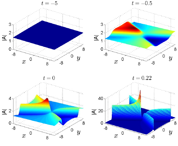
It is interesting to compare this fundamental rogue wave of the nonlocal DSI equation with that of the local DSII equation YangDSII . First of all, the parameter conditions are very different. In the local DSII equation, rogue waves require ; if , the rational solution would be a two-dimensional lump moving on a constant background. In the nonlocal DSI equation (2), rogue waves require to be purely imaginary. In this case, generically, and thus the transformations (II.8) convert moving-lump solutions of the local DSII equation into rogue waves of the nonlocal DSI equation. Secondly, in the local DSII equation, rogue waves exist only when ; but in the nonlocal DSI equation (2), rogue waves exist for both signs of nonlinearity . Thirdly, in the local DSII equation, fundamental rogue waves are line rogue waves; but in the nonlocal DSI equation, fundamental rogue waves have richer structures. Fourthly, in the local DSII equation, fundamental rogue waves never blow up in finite time; but in the nonlocal DSI equation, fundamental rogue waves generically blow up in finite time. Although some non-generic multi-rogue waves and higher-order rogue waves of the local DSII equation can also blow up in finite time, they only do so at a single spatial point, unlike the fundamental rogue waves of the nonlocal DSI equation where the blowup occurs on an entire hyperbola of the spatial plane.
Multi-rogue waves of the nonlocal DSI equations (2) can be similarly derived from those of the local DSII equations in Satsuma_Ablowitz ; YangDSII under the reverse variable transformations , , and the parameter conditions of being purely imaginary. These multi-rogue waves describe the nonlinear interaction of several individual fundamental rogue waves. Details are omitted.
III.2 Partially -symmetric DSII equations
Rogue waves in partially -symmetric DSII equations (2), with , can be obtained from the rational solutions in the local DSI equations (2) under the reverse of transformations (II.8). These rational solutions in the local DSI equations have been reported in Satsuma_Ablowitz ; YangDSI . Imposing suitable parameter restrictions, rogue waves in the nonlocal DSII equations (2) will be obtained.
Fundamental rational solutions in the nonlocal DSII equations (2) can be obtained from analogous solutions in Ref. YangDSI for the local DSI equations under the reverse variable transformations , , , and accounting for the sign switching of the nonlinearity parameter . These fundamental rational solutions of the nonlocal DSII equations are given by the same formulae (III.1)-(III.5), except that the expressions for parameters and are different:
| (III.8) |
As before, and are free complex constants. Analysis of these rational solutions shows that they become rogue waves when and , in which case are imaginary and real. These rogue waves approach a constant background as , but develop finite-time singularity at time and on the hyperbola
| (III.9) |
Graphs of these rogue waves are qualitatively similar to those in Fig. 1.
Multi-rogue waves in the nonlocal DSII equations (2) can be derived from those of the local DSI equations in Satsuma_Ablowitz ; YangDSI under variable transformations and parameter conditions of , . Details are omitted.
IV Rogue waves in the nonlocal derivative NLS equation
Now, we consider rogue waves in the nonlocal derivative NLS equation (II.10), i.e.,
| (IV.1) |
where . These rogue waves can be obtained from rational solutions of the local derivative NLS equation (II.12) through the variable transformation (II.11). This local equation is invariant when , thus we fix without loss of generality. For this value, the fundamental rational solution in the local derivative NLS equation is given by Eq. (47) in Ref. GuoDNLS , and it is a moving soliton on a constant background. Then under the reverse of the transformation (II.11), i.e., , , this moving soliton of the local equation is converted to the following fundamental rational solution of the nonlocal equation,
| (IV.2) |
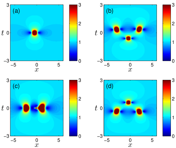
The graph of this solution is displayed in Fig. 2(a). It is seen that this is a rogue wave, rising from a constant background and then retreating back to the same background, analogous to the Peregrine solution of the NLS equation. However, the present rogue wave blows up to infinity at and finite time , unlike the Peregrine solution.
Higher-order rogue waves in the nonlocal equation (IV.1) can be obtained from higher-order rational solutions of the local derivative NLS equation. For instance, the second-order rational solution of the local equation is given by Eq. (48) in Ref. GuoDNLS . Then under the transformations , , we get the second-order rational solution of the nonlocal equation (IV.1) as
| (IV.3) |
where
and is a free real constant. Graphs of these rational solutions are plotted in Fig. 2(b,c,d) for and respectively. It is seen that these rational solutions are second-order rogue waves which arise from and retreat back to the same constant background. But they blow up to infinity at three points of the plane.
V Multi-solitons and quasi-periodic solutions in the reverse space-time CMKdV equation
In this section, we derive analytical solutions for the reverse space-time CMKdV equation (II.13), i.e.,
| (V.1) |
where . The case of will be called the focusing case, and that of the defocusing case. As we have shown, this nonlocal equation, under transformations (II.14), becomes the local CMKdV equation (II.15) with the opposite sign of nonlinearity. Thus, we will derive analytical solutions for the defocusing/focusing nonlocal CMKdV equation from those of the local focusing/defocusing CMKdV equation.
V.1 Multi-solitons in the nonlocal focusing equation
Eq. (V.1) in the focusing case has . Solitons and multi-solitons in this nonlocal focusing equation can be constructed from singular solutions in the local defocusing equation (II.15). The local defocusing equation admits the following singular solutions
| (V.2) |
where , and are real constants. Then under the reverse of transformations (II.14), i.e., , , this singular solution becomes
| (V.3) |
which is the fundamental soliton in the nonlocal focusing CMKdV equation (V.1). Its peak amplitude, which occurs at , is . Thus, for a given , this peak amplitude can vary from to infinity depending on the choice of the values.
Second-order singular solutions in the local defocusing equation (II.15) can be obtained from Ref. CMKdV2soliton under certain parameter constraints [specifically, by requiring negative in Eq. (3.18) of that paper]. Then, under the above variable transformations, we get two-soliton solutions in the nonlocal focusing CMKdV equation (V.1) as
| (V.4) |
with
For parameter choices
| (V.5) |
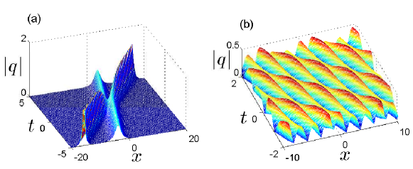
this two-soliton solution is displayed in Fig. 3(a).
Higher-order solitons in the nonlocal focusing CMKdV equation (V.1) can be obtained similarly.
V.2 Quasi-periodic solutions in the nonlocal defocusing equation
Eq. (V.1) in the defocusing case has . In this case, the local focusing CMKdV equation (II.13) has a soliton solution
| (V.6) |
where and are real constants. Then under the transformations, we obtain the following solution for the nonlocal defocusing equation (V.1),
| (V.7) |
This solution is a traveling wave and is periodic in both space and time .
Second-order extensions of this periodic solution can be obtained from two-soliton solutions of the local focusing CMKdV equation. The latter can be found in Eq. (3.18) of Ref. CMKdV2soliton . Then, under variable transformations , , we get the following solution for the defocusing nonlocal CMKdV equation (V.1) as
| (V.8) |
where
This solution contains two frequencies and is generically quasi-periodic in both space and time. Under the parameter choices
| (V.9) |
this double-frequency quasi-periodic solution is displayed in Fig. 3(b).
Higher-order quasi-periodic solutions in the nonlocal defocusing CMKdV equation (V.1) can be obtained from higher-order solitons of the local focusing CMKdV equation in a similar way.
VI New nonlocal integrable equations
In this last section, we show how these variable transformations can be used to derive new integrable nonlocal equations from their local counterparts.
VI.1 Nonlocal complex short pulse equations
As the first example, we consider the integrable local complex short pulse (CSP) equation Feng_shortpulse ; Feng3 ,
| (VI.1) |
where is a complex function. Under variable transformations , we get an integrable reverse space nonlocal CSP equation,
| (VI.2) |
Under a different variable transformation , we get an integrable reverse time nonlocal CSP equation,
| (VI.3) |
Under the combined transformations , we get an integrable reverse space-time nonlocal CSP equation,
| (VI.4) |
Notice that this last nonlocal equation admits a reduction of being real-valued. Under this reduction, we get an integrable reverse space-time real short-pulse equation
| (VI.5) |
where is a real function.
Infinite numbers of conservation laws for these new nonlocal short-pulse equations can be inferred directly from those of local short-pulse equations through the corresponding variable transformations. For instance, the first two conserved quantities of the local CSP equation (VI.1) are
| (VI.6) | |||||
| (VI.7) |
The former quantity has been reported in Feng_shortpulse ; Feng3 , and we found the latter quantity by inspiration of conserved quantities for the Wadati-Konno-Ichikawa hierarchy (which contains the real short pulse equation) Franca2012 . Then, using these conserved quantities and the transformation , we obtain the first two conserved quantities of the reverse space nonlocal CSP equation (VI.2) as
| (VI.8) | |||||
| (VI.9) |
Under the transformation , we obtain the first two conserved quantities of the reverse time nonlocal CSP equation (VI.3) as
| (VI.10) | |||||
| (VI.11) |
Under the combined transformations , we obtain the first two conserved quantities of the reverse space-time nonlocal CSP equation (VI.4) as
| (VI.12) | |||||
| (VI.13) |
The first two conserved quantities of the reverse space-time real short-pulse equation (VI.5) are simply these in (VI.12)-(VI.13) with the complex conjugate removed.
Higher conserved quantities of these new nonlocal CSP equations can be similarly obtained.
VI.2 Nonlocal nonlinear diffusion equations
As a second example, we consider the local integrable NLS equation
| (VI.14) |
Under the variable transformation , we get an integrable reverse time nonlinear diffusion equation
| (VI.15) |
Under the variable transformations , we get an integrable reverse space-time nonlinear diffusion equation
| (VI.16) |
Notice that both of these nonlocal equations admit the reduction of being real. Under this reduction, we also obtain integrable reverse-time and reverse-space-time real nonlinear diffusion equations
| (VI.17) |
and
| (VI.18) |
Infinite numbers of conservation laws for these new nonlocal diffusion equations can be readily derived from those of the local NLS equation (VI.14) through variable transformations. For instance, using the first four conserved quantities of the local NLS equation Yang2010 , we immediately obtain the first four conserved quantities of the reverse time nonlinear diffusion equation (VI.15) as
Likewise, the first four conserved quantities of the reverse space-time nonlinear diffusion equation (VI.16) are found to be
Conserved quantities for the reverse-time and reverse-space-time real nonlinear diffusion equations (VI.17)-(VI.18) are simply those of the complex equations above with the conjugation removed.
Analytical solutions to these nonlocal diffusion equations can also be derived from solutions of the local NLS equation through transformations. For example, from the soliton solution of the local focusing NLS equation (VI.14),
| (VI.19) |
with being real constants, we obtain the solution to the reverse time nonlocal diffusion equation (VI.15) with as
| (VI.20) |
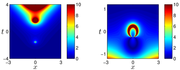
This solution exponentially grows or decays depending on the sign of . In addition, it periodically collapses at location . For , this solution is illustrated in Fig. 4 (left panel).
As another example, from the Peregrine rogue wave solution of the local focusing NLS equation (VI.14),
| (VI.21) |
and utilizing the transformations , we obtain the following solution to the reverse space-time nonlocal diffusion equation (VI.16) with as
| (VI.22) |
This solution is illustrated in Fig. 4 (right panel). It decays exponentially with time, but blows up to infinity on the ellipse of the plane.
VI.3 Other new nonlocal integrable equations
In addition to the above new nonlocal integrable equations, we can also obtain many other such equations using transformations. For instance, from the local Sasa-Satsuma equation SS
| (VI.23) |
and employing the variable transformations , we get an integrable reverse space-time Sasa-Satsuma equation,
| (VI.24) |
From the local Chen-Lee-Liu equation ChenLeeLiu
| (VI.25) |
and employing the variable transformation , we obtain an integrable reverse-space Chen-Lee-Liu equation
| (VI.26) |
A different transformation yields a different integrable reverse-space-time nonlinear diffusion equation
| (VI.27) |
From the local modified NLS equation WadatiMNLS
| (VI.28) |
with real constants , and under transformations , we get an integrable reverse-space modified NLS equation
| (VI.29) |
From an integrable (2+1)-dimensional NLS equation 2DNLS_lump_rogue
| (VI.30) |
and taking the transformations , we obtain an integrable reverse-space (2+1)-dimensional NLS equation
| (VI.31) |
Thus, this transformation technique is a powerful tool to generate a large class of new nonlocal integrable equations. Solution dynamics in these new nonlocal equations can also be studied through this transformation, as we have demonstrated earlier in this article.
VII Summary
In summary, we have reported that many recently proposed nonlocal integrable equations can be converted to local integrable equations through simple variable transformations. Examples include -symmetric NLS and Davey-Stewartson equations, a nonlocal derivative NLS equation, the reverse space-time complex modified Korteweg-de Vries equation, reverse space-time three wave interaction equations, and many others. These transformations not only establish the integrability of these nonlocal equations, but also allow us to construct their analytical solutions from solutions of the local equations. These transformations can also be used to derive new nonlocal integrable equations. As applications of these transformations, we have used them to derive rogue wave solutions for the partially -symmetric Davey-Stewartson equations and the nonlocal derivative NLS equation. In addition, we have used them to derive multi-soliton and quasi-periodic solutions in the reverse space-time complex modified KdV equation. Furthermore, we have used them to construct many new nonlocal integrable equations such as nonlocal short pulse equations, nonlocal nonlinear diffusion equations, nonlocal Sasa-Satsuma equations and nonlocal Chen-Lee-Liu equations.
These transformations reveal an intimate and deep connection between many nonlocal and local integrable equations. They are expected to provide a new and powerful tool in the study of these nonlocal equations.
Acknowledgment
This material is based upon work supported by the Air Force Office of Scientific Research under award number FA9550-12-1-0244, and the National Science Foundation under award number DMS-1616122. The work of B.Y. is supported by a visiting-student scholarship from the Chinese Scholarship Council.
References
References
- (1) M.J. Ablowitz and H. Segur, Solitons and Inverse Scattering Transform (SIAM, Philadelphia, 1981).
- (2) S.P. Novikov, S.V. Manakov, L.P. Pitaevskii and V.E. Zakharov, Theory of Solitons (Plenum, New York, 1984)
- (3) L. Takhtadjan and L. Faddeev, The Hamiltonian Approach to Soliton Theory (Springer Verlag, Berlin, 1987).
- (4) M.J. Ablowitz and P.A. Clarkson, Solitons, Nonlinear Evolution Equations and Inverse Scattering (Cambridge University Press, 1991).
- (5) J. Yang, Nonlinear Waves in Integrable and Non integrable Systems (SIAM, Philadelphia, 2010).
- (6) M.J. Ablowitz and Z.H. Musslimani, “Integrable nonlocal nonlinear Schrödinger equation”, Phys. Rev. Lett. 110, 064105 (2013).
- (7) M.J. Ablowitz and Z.H. Musslimani, “Integrable discrete symmetric model”, Phys. Rev. E 90, 032912 (2014).
- (8) Z. Yan, “Integrable -symmetric local and nonlocal vector nonlinear Schrödinger equations: A unified two-parameter model,” Appl. Math. Lett. 47, 61–68 (2015).
- (9) A. Khara and A. Saxena, “Periodic and hyperbolic soliton solutions of a number of nonlocal nonlinear equations”, J. Math. Phys. 56, 032104 (2015).
- (10) M.J. Ablowitz and Z.H. Musslimani, “Inverse scattering transform for the integrable nonlocal nonlinear Schrödinger equation,” Nonlinearity 29, 915–946 (2016).
- (11) C.Q. Song, D.M. Xiao and Z.N. Zhu, “Solitons and dynamics for a general integrable nonlocal coupled nonlinear Schrödinger equation”, Commun. Nonlinear Sci. Numer. Simul. 45, 13–28 (2017).
- (12) A.S. Fokas, “Integrable multidimensional versions of the nonlocal nonlinear Schrödinger equation”, Nonlinearity 29, 319–324 (2016).
- (13) S.Y. Lou, “Alice-Bob systems, -- principles and multi-soliton solutions”, https://arxiv.org/abs/1603.03975 (2016).
- (14) S.Y. Lou and F. Huang, “Alice-Bob physics: coherent solutions of nonlocal KdV systems”, Scientific Reports 7, 869 (2017).
- (15) M.J. Ablowitz and Z.H. Musslimani, “Integrable nonlocal nonlinear equations”, Stud. Appl. Math. DOI: 10.1111/sapm.12153 (2016).
- (16) Z.X. Xu, and K.W. Chow, “Breathers and rogue waves for a third order nonlocal partial differential equation by a bilinear transformation”, Appl. Math. Lett. 56, 72–77 (2016).
- (17) Z.X. Zhou, “Darboux transformations and global solutions for a nonlocal derivative nonlinear Schrödinger equation”, arXiv:1612.04892 [nlin.SI] (2016).
- (18) Z.X. Zhou, “Darboux transformations and global explicit solutions for nonlocal Davey-Stewartson I equation”, arXiv:1612.05689 [nlin.SI] (2016).
- (19) J.G. Rao, Y.S. Zhang, A.S. Fokas, and J.S. He, “Rogue waves of the nonlocal Davey-Stewartson I equation” (preprint 2016).
- (20) J.G. Rao, Y. Cheng and J.S. He, “Rational and semi-rational solutions of the nonlocal Davey-Stewartson equations”, to appear in Stud. Appl. Math. (2017).
- (21) J.L. Ji and Z.N. Zhu, “On a nonlocal modified Korteweg-de Vries equation: integrability, Darboux transformation and soliton solutions”, Commun. Nonlinear Sci. Numer. Simul. 42 699–708 (2017).
- (22) L.Y. Ma, S.F. Shen and Z.N. Zhu, “Integrable nonlocal complex mKdV equation: soliton solution and gauge equivalence”, arXiv:1612.06723 [nlin.SI] (2016).
- (23) V. S. Gerdjikov and A. Saxena, “Complete integrability of nonlocal nonlinear Schrödinger equation”, J. Math. Phys. 58, 013502 (2017).
- (24) M.J. Ablowitz, X. Luo, and Z.H. Musslimani, “Inverse scattering transform for the nonlocal nonlinear Schrödinger equation with nonzero boundary conditions”, arXiv:1612.02726 [nlin.SI] (2016).
- (25) S.V. Suchkov, A.A. Sukhorukov, J. Huang, S.V. Dmitriev, C. Lee and Y.S. Kivshar, “Nonlinear switching and solitons in -symmetric photonic systems”, Laser Photonics Rev. 10, 177 (2016).
- (26) V.V. Konotop, J. Yang and D.A. Zezyulin, “Nonlinear waves in -symmetric systems,” Rev. Mod. Phys. 88, 035002 (2016).
- (27) T.A. Gadzhimuradov and A.M. Agalarov, “Towards a gauge-equivalent magnetic structure of the nonlocal nonlinear Schrödinger equation”, Phys. Rev. A 93, 062124 (2016).
- (28) D.J. Kaup and A.C. Newell, “An exact solution for a derivative nonlinear Schrödinger equation”, J. Math. Phys. 19, 798 (1978).
- (29) J. Satsuma and M.J. Ablowitz, “Two-dimensional lumps in nonlinear dispersive systems”, J. Math. Phys. 20, 1496–503 (1979).
- (30) Y. Ohta and J. Yang, “Dynamics of rogue waves in the Davey-Stewartson II equation”, J. Phys. A 46, 105202 (2013).
- (31) D.H. Peregrine, “Water waves, nonlinear Schrödinger equations and their solutions”, J. Aust. Math. Soc. B 25, 16–43 (1983).
- (32) Y. Ohta and J. Yang, “Rogue waves in the Davey-Stewartson-I equation”, Phys. Rev. E 86, 036604 (2012).
- (33) B. Guo, L. Ling, and Q.P. Liu, “High-order solutions and generalized Darboux transformations of derivative nonlinear Schrödinger equations”, Stud. Appl. Math. 130, 317–344 (2013).
- (34) S. C. Anco, N. T. Ngatat and M. Willoughby, “Interaction properties of complex modified Korteweg de Vries (mKdV) solitons”, Physica D, 240, 1378–1394 (2011).
- (35) B.F. Feng, “Complex short pulse and coupled complex short pulse equations,” Physica D 297, 62–75 (2015).
- (36) B.F. Feng, K. Maruno and Y. Ohta, “Geometric formulation and multi-dark soliton solution to the defocusing complex short pulse equation”, Stud. Appl. Math. 138, 343–367 (2017).
- (37) G.S. Franca, J.F. Gomes and A.H. Zimerman, “The higher grading structure of the WKI hierarchy and the two-component short pulse equation”, J. High Energ. Phys. 2012:120, doi:10.1007/JHEP08(2012)120 (2012).
- (38) N. Sasa and J. Satsuma, “New type of soliton solutions for a higher-order nonlinear Schrodinger equation”, J. Phys. Soc. Jpn. 60, 409 (1991).
- (39) H.H. Chen, Y.C. Lee and C.S. Liu, “Integrability of nonlinear Hamiltonian system by inverse scattering method”, Phys. Scr. 20, 490–492 (1979).
- (40) M. Wadati, K. Konno, and Y.H. Ichikawa, “A generalization of inverse scattering method”, J. Phys. Soc. Jpn. 46, 1965 (1979).
- (41) A. Kundu, A. Mukherjee and T. Naskar, “Modelling rogue waves through exact dynamical lump soliton controlled by ocean currents”, Proc. R. Soc. A 470, 20130576 (2014).