Indoor Frame Recovery from Refined Line Segments

Abstract

An important yet challenging problem in understanding indoor scene is recovering indoor frame structure from a monocular image. It is more difficult when occlusions and illumination vary, and object boundaries are weak. To overcome these difficulties, a new approach based on line segment refinement with two constraints is proposed. First, the line segments are refined by four consecutive operations, i.e., reclassifying, connecting, fitting, and voting. Specifically, misclassified line segments are revised by the reclassifying operation; some short line segments are joined by the connecting operation; the undetected key line segments are recovered by the fitting operation with the help of the vanishing points; the line segments converging on the frame are selected by the voting operation. Second, we construct four frame models according to four classes of possible shooting angles of the monocular image, the natures of all frame models are introduced via enforcing the cross ratio and depth constraints. The indoor frame is then constructed by fitting those refined line segments with related frame model under the two constraints, which jointly advance the accuracy of the frame. Experimental results on a collection of over 300 indoor images indicate that our algorithm has the capability of recovering the frame from complex indoor scenes.

1 Introduction

Understanding indoor scene has been a popular research subject over the past decade. An important aspect of understanding indoor scene is the recovery of an indoor frame from a monocular image. Yet, indoor frame recovery remains a challenging task because some extreme difficulties, such as variations in occlusions and illumination and weak object boundaries. As a result, the extraction of line segements can be affected. For example, a mess of line segments are detected, with many noisy line segments. On the other hand, some key line segments may be undetected (Fig. 1a). Therefore, recovering correct indoor frame from those messy line segments is a complicated task.

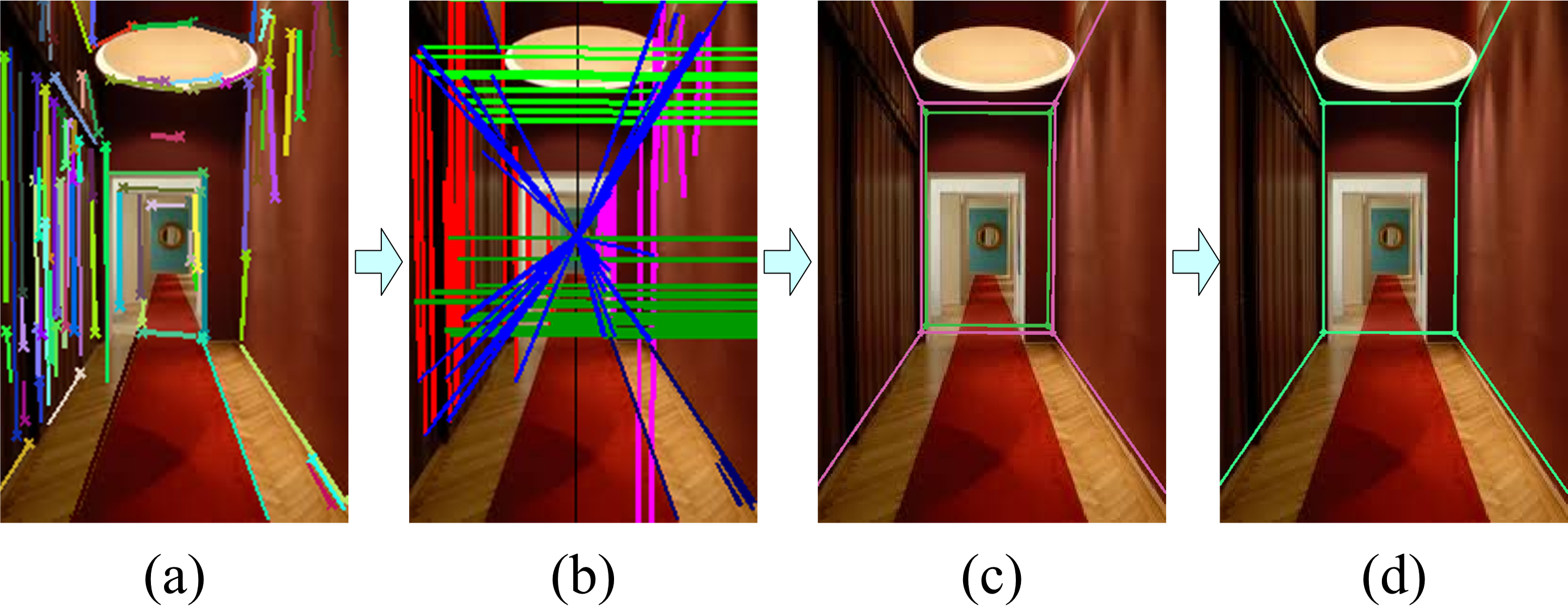
Figure 1: Overview of our work. (a) The initial line segments, which extracted by a pervasive algorithm proposed by P. Kovesi [13]. (b) The refined line segments after reclassifying, connecting, fitting, and voting. (c) The candidate frames by enforcing a cross ratio constraint. (d) The final frame by adding a depth constraint.

Circumscribed by the Manhattan assumption, the goal of our work is to recover the frames from line segments, which are affected by various degrees of occlusion and by illumination in indoor scenes.

In this paper, we tackle the task from a new sight. We transfer the problem of recognizing the indoor frame from these line segments into analyzing the relationships between these lines and points. Two new concepts (Sec. 3.2), box line and supporting point, are introduced for this transfermation. We then describe four properties of the box line and supporting point (Sec. 3.2). Successively, we derive strategies such as reclassifying, connecting, fitting, and voting, and constraints such as cross ratio and depth from the properties of the box line and supporting point. Besides the two new concepts, we construct four frame models according to four classes of possible shooting angles of the monocular image (Sec. 3.1). The two natures of four frame models are presented as the cross ratio and depth constraints. Finally, we refine the initial line segments and construct the indoor frame through these strategies and constraints with related frame model.

The main contribution of this paper can be summarized into two parts. First, through the refining process, we improve the initial line segments greatly. Especially, our method can estimate undetected key line segments on weak object boundaries and occluded regions (Fig. 9b & Fig. 10b), which could not be estimated via using other approaches of indoor frame recovery [15, 10]. Second, the cross ratio and depth constraints (i.e., the two natures of frames) enable us to recover the frame more accurately than [15] and [10], especially when the object boundaries are weak, the illumination varies, and occlusions exist in the indoor scene. Besides, because the solution space is first decreased in voting process of line segment refinement, then further limited by the cross ratio and depth constraints, we can recover the frame more rapidly, as shown in Table 2.

A preliminary version of this work appeared in [3]. This article extends the conference version of [3], with four kinds of frame models instead of the crab-like model, and a depth constraint as a complement, and discussions of applications and limitations.

2 Related Work

As the need of some indoor applications (i.e., robot navigation, object recognition, 3D reconstruction, and event detection [12, 8, 2, 24, 21, 18, 7, 9, 11, 26, 14, 20, 23]), understanding indoor scenes comes into eyes of researchers. Consequently, many algorithms of indoor frame recovery have been proposed. From the perspective of feature utilization, recent work can be classified into two main groups: texture-based and line segment-based.

Texture-based approaches often over-segment the image into patches first and then label each patch according to two descriptors: the color histogram and the texture histogram. For example, Liu et al. [16] over-segmented an image by using the graph cut and then introduced texture to label the frame. However, the texture descriptors of indoor scenes are sensitive to illumination variations. Moreover, the texture descriptors of ceilings, floors, and walls are often similar to one another in indoor scenes, such that the discrimination level of these descriptors is low. Therefore, methods based on texture descriptors usually cannot work well when applied to indoor images. Silberman et al. [24] and Ren et al. [21] introduced depth to determine the category of each pixel based on an RGB-D image. These methods often segment the planes of indoor images according to the depth of each plane. Unlike the texture descriptors, the depth descriptor is insensitive to illumination variations. Admittedly, depth is useful in indoor frame recovery, yet, it is hard to obtain accurate depth information pragmatically.

Given that texture-based approaches are sensitive to illumination variations and there is low discrimination on indoor images, numerous line segment-based approaches have been proposed [19, 27]. Compared with texture-based algorithms, line segment-based approaches have three advantages: (1) excellent information on the building structure, (2) minimal impact of the distance between the camera and scene on line segments, and (3) robust to illumination variations. Lee et al. [15] proposed a corner model of twelve statuses to fit the frame through line segments. After them, Hedau et al. [10] generated candidate frames by shooting rays from vanishing points and then selected the best candidate via ranking support vector machines (SVMs). Further more, Flint et al. [6] employed a visual simultaneous localization and mapping system to refine the frame locally. However, these line segment-based algorithms often do not work well when abundant, or missing, or incorrect extraction, appears in the detected line segments.

To address that, some approaches of refining line segments have been put forward. Pero et al. [19] used the location of corners to delete useless line segments. However, in practice, the corners are usually occluded by furniture. Therefore, cues based methods appear. Hedau et al. [10] labeled the furniture as cues to filter line segments. But no matter how to select from those messy line segments, which still have not been refined radically.

To improve the quality of these messy line segments, some effective measures (i.e., reclassifying, connecting, fitting, and voting) have been proposed in this paper (Sec. 4). The first two are relatively simple, the last two are derived from two properties ($\mathbf{R_{1}}$ and $\mathbf{R_{2}}$) of the new concepts of box line and supporting point (Sec. 3.2). After obtaining refined line segments, constructing the frame becomes much easier. We construct four frame models according to four classes of possible shooting angles of the monocular image. With the help of one of the four frame models, and reinforced by two natures of frames (i.e., cross ratio constraint and depth constraint), we fit the refined line segments to generate the frame.

3 Definitions and Notations

3.1 Frame & Frame model

The frame of an indoor scene is a structure, which consists of intersections of ceiling, floor, and walls.The structural integrity of the indoor scene varies with the shooting angle. In practice, only 4 (2 or 1) corners of the frame can be seen from the input images of indoor scenes (Fig. 2). Therefore, we propose four frame models ”4c”, ”2vc”, ”1c”, and ”2hc” to represent four levels of integrity of the frame structures of these indoor scenes (Fig. 2). The front number stands for the number of the corners appearing on the input images. The letter ”c” represents the corner. The letter ”v” of ”2vc” means the line across the two corners is in the vertical orientation. Similarly, the letter ”h” of ”2hc” means the horizontal orientation. The frame models of ”4c”, ”2vc”, ”1c”, and ”2hc” consist of eight lines, five lines, three lines, and five lines, respectively. The notations used to parametrize the frame models are described as follows:

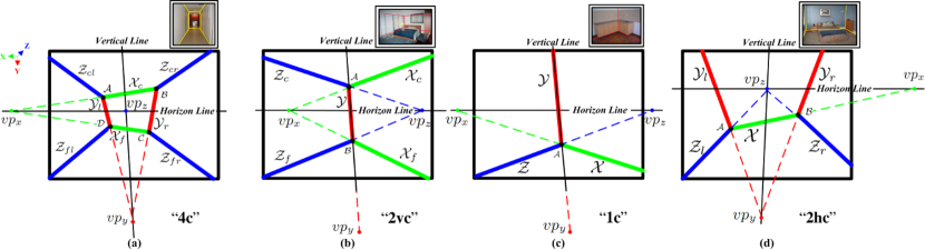
Figure 2: Four frame models, named ”4c”, ”2vc”, ”1c”, and ”2hc”. The front number stands for the number of the corners appearing on the input images. The letter ”c” represents the corner. The letter ”v” of ”2vc” means the line across the two corners is in the vertical orientation. Similarly, the letter ”h” of ”2hc” means the horizontal orientation. The frame models of ”4c”, ”2vc”, ”1c”, and ”2hc” consist of eight lines, five lines, three lines, and five lines, respectively.

1. We denote three vanishing points of the mutually orthogonal $x$, $y$, and $z$ orientations as $vp_{x}$, $vp_{y}$, and $vp_{z}$, respectively. The line passing through $vp_{y}$ and $vp_{z}$ is denoted as the vertical line $l_{yz}$, and that through $vp_{x}$ and $vp_{z}$ is denoted as the horizontal line $l_{xz}$. We also denote the line passing through $vp_{x}$ and $vp_{y}$ as $l_{xy}$ (Fig. 2).

2. For all frame models, the detected line segments are partitioned into three sets, $\mathcal{X}$, $\mathcal{Y}$, and $\mathcal{Z}$, according to three vanishing points. Further, $\mathcal{X}$, $\mathcal{Y}$, and $\mathcal{Z}$ are assigned into eight subsets, $\mathcal{X}_{c}$, $\mathcal{X}_{f}$, $\mathcal{Y}_{l}$, $\mathcal{Y}_{r}$, $\mathcal{Z}_{cl}$, $\mathcal{Z}_{cr}$, $\mathcal{Z}_{fr}$, and $\mathcal{Z}_{fl}$, in ”4c”, by the coordinate axis of $l_{yz}$ and $l_{xz}$; those are assigned into five subsets, $\mathcal{X}_{c}$, $\mathcal{X}_{f}$, $\mathcal{Y}$, $\mathcal{Z}_{c}$, and $\mathcal{Z}_{f}$, in ”2vc”, by the axis of $l_{xz}$; those are also assigned into five subsets, $\mathcal{X}$, $\mathcal{Y}_{l}$, $\mathcal{Y}_{r}$, $\mathcal{Z}_{l}$, and $\mathcal{Z}_{r}$, in ”2hc”, by the axis of $l_{yz}$; those still maintain $\mathcal{X}$, $\mathcal{Y}$, and $\mathcal{Z}$ in ”1c”. In those subsets, right subscripts $"c"$, $"f"$, $"l"$, $"r"$, $"cl"$, $"cr"$, $"fr"$, and $"fl"$ stand for meanings of ceiling, floor, left, right, ceiling_left, ceiling_right, floor_right, and floor_left, respectively. $\mathcal{A}$, $\mathcal{B}$, $\mathcal{C}$, and $\mathcal{D}$ denote the corners, there are 4, 2, 2, 1 corners in ”4c”, ”2hc”, ”2vc”, and ”1c”, respectively (Fig. 2).

3.2 Box Line & Supporting Point

Most people utilize the information obtained from a line segment itself (i.e., length, location, etc.), but often ignore the relationship between the line segment and others. Relationships between a line segment and its vanishing point have been studied a lot [22, 1, 25]. However, other relationships between related lines and points have not been studied yet (except the simple geometric relationship). In order to address these relationships, new concepts of box line and supporting point are proposed.

A box line is a line segment on the frame, such that if it intersects with another line segment, the interseting point is the end point of that line segment. A supporting point is an endpoint of a line segment on the box line. It seems as if the box line is supported by the line segment, one of whose endpoints is on the box line. Therefore, the endpoint of that line segment is named supporting point. Box line is obviously important because frame is derived from them. Supporting point can be matched with the box line, because the relationships among the box lines and supporting points are significant, yet rarely noted by people, which can be summarized as the following four items.

$\mathbf{R_{1}}$: a supporting point exists because a box line blocks the extension of some line segment. (Sec. 4.3, Fig. 5)

$\mathbf{R_{2}}$: any line segment cannot penetrate the boundary of the planes (the box lines). (Sec. 4.4, Fig. 6)

$\mathbf{R_{3}}$: there is a cross ratio invariance among the box lines (the frame). (Sec. 5.1)

$\mathbf{R_{4}}$: the distance between the intersection of the box lines (corner of the frame) and the camera is the longest among the distances between the camera and other points nearby. (Sec. 5.2, Fig. 8)

One supporting point corresponds to one box line, yet one box line corresponds to more than one supporting point. Before we obtain the group of box lines. we only have the groups of candidate box lines, where there are lots of noisy line segments, and the related groups of candidate supporting points. Therefore, we refine and reduce the groups of candidate box lines with above four natures, until the box lines are winkled out.

4 Line Segment Refinement

In our method, line segments are initialized by the detector proposed in [13]. By using the vanishing point estimation algorithm proposed in [25], we obtain the three vanishing points $vp_{x}$, $vp_{y}$, and $vp_{z}$ and then divide the initial line segments into three sets: $\mathcal{X}$, $\mathcal{Y}$, and $\mathcal{Z}$. However, the frame can hardly be recovered directly from the three sets of line segments because these sets often have the following problems:

First, by using the algorithm proposed by J. Tardif [25], the line segments nearly paralleling to $l_{xz}$ and $l_{yz}$ are often misclassified. Second, given the illumination variations and the existing of occlusions, long line segments are often not detected, instead, divided into many parts. Third, edges on weak object boundaries often cannot be detected as line segments, therefore, some important line segments are often lost. Fourth, traversing the entire set of line segments, which include many non-essential redundancies, increases the computational complexity.

For the first two difficulties, we propose two operations, reclassifying and connecting, on the sets of $\mathcal{X}$, $\mathcal{Y}$, and $\mathcal{Z}$. According to manually given cue of the category of used frame model, ”4c”, or ”2vc”, or ”2hc”, or ”1c”, we then further assign sets of $\mathcal{X}$, $\mathcal{Y}$, and $\mathcal{Z}$ into subsets. For category of ”4c”, or ”2vc”, or ”2hc”, the detected line segments are further partitioned into 8, 5, 5 subsets, respectively. While for category of ”1c”, we maintain the three sets, $\mathcal{X}$, $\mathcal{Y}$, and $\mathcal{Z}$. To overcome the last two difficulties, for each category, we implement measures of fitting and voting on subsets (sets, when ”1c”), with first two natures of box lines and supporting points.

4.1 Reclassifying

To address the first problem, we use neighbor assignment to reclassify a line segment $l$. Especially, for each line segment $l$ in $\mathcal{X}$ and $\mathcal{Z}$, we calculate the angle $\theta$ between $l$ and $l_{xz}$. If $\theta<\tau_{\theta}=20^{\circ}$, we use nearest neighbor assignment to reclassify the line segment $l$, as described in Fig. 3. For more details, assuming that the $\theta$ between $x_{1}$ ($x_{1}$ is a line segment in $\mathcal{X}$) and $l_{xz}$ is less than $\tau_{\theta}$, then we construct a round neighborhood of $x_{1}$, taking the midpoint of $x_{1}$ as the center and half-length of $x_{1}$ as the radius. We then search $\mathcal{Z}$ to find whether there are $n>2$ line segments of $\mathcal{Z}$ intersecting with the round neighborhood, if so, we reclassify $x_{1}$ to $\mathcal{Z}$. Otherwise, we maintain its own status. The treatments of line segments in $\mathcal{Y}$ and $\mathcal{Z}$ are similar with that. After reclassifying, $\mathcal{X}$, $\mathcal{Y}$, and $\mathcal{Z}$ are refreshed.

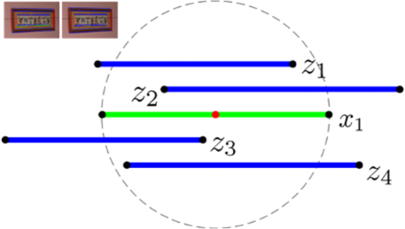
Figure 3: A sketch to illustrate the neighbor assignment of reclassification. There are four line segments of $\mathcal{Z}$ intersect with the neighborhood of $x_{1}$, therefore, $x_{1}$ should be reclassified to $\mathcal{Z}$. the miniature image of upper-left is an actual example.

4.2 Connecting

Collinearity is used to address the second problem, that is checking whether two line segments are collinear. For any two line segments $l_{i}$ and $l_{j}$ from $\mathcal{X}$ ($\mathcal{Y}$ or $\mathcal{Z}$), the sum of their length is calculated as $length=\textrm{len}(l_{i})+\textrm{len}(l_{j})$, where $\textrm{len}(\cdot)$ is the length function at pixel level. Then we calculate the longest distance (lDis) and shortest distance (sDis) between the pixels of $l_{i}$ and those of $l_{j}$. Finally, we calculate the collinearity error as,

$$e=|lDis-sDis-length|,$$ (1)

If $e<\tau_{e}=0.3$, we connect the two line segments $l_{i}$ and $l_{j}$ as a new line segment. Otherwise, let them remain themselves. Consequently, $\mathcal{X}$, $\mathcal{Y}$, and $\mathcal{Z}$ are refreshed again.

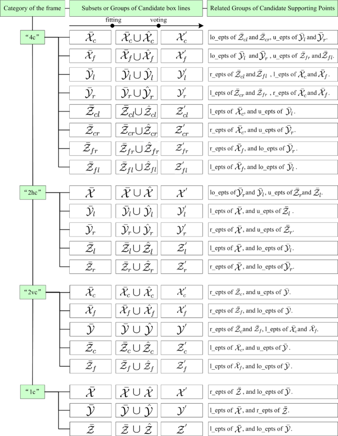
Figure 4: The figure shows the correspondences between the groups of candidate box lines and the related groups of candidate supporting points, for each category of the frame models. In the figure, l_epts, r_epts, u_epts, and lo_epts are compact forms of left endpoints, right endpoints, upper endpoints, and lower endpoints. Taking ”4c” as an example, after reclassifying and connecting and before fitting, there are eight subsets or groups of candidate box lines, such as $\bar{\mathcal{X}}_{c}$. While after the fitting operation, $\bar{\mathcal{X}}_{c}$ turns to $\bar{\mathcal{X}}_{c}\cup\hat{\mathcal{X}}_{c}$, where $\hat{\mathcal{X}}_{c}$ is the set of added line segments. Further, after the voting operation, $\bar{\mathcal{X}}_{c}\cup\hat{\mathcal{X}}_{c}$ decreases to $\mathcal{X}_{c}^{{}^{\prime}}$, for iteratively voting selection. On the other hand, the related groups of candidate supporting points remain the same, until the end of the voting process. For example, for $\bar{\mathcal{X}}_{c}$ or $\bar{\mathcal{X}}_{c}\cup\hat{\mathcal{X}}_{c}$, the related groups of supporting points are lo_epts of $\bar{\mathcal{Z}}_{cl}$ and $\bar{\mathcal{Z}}_{cr}$, and u_epts of $\bar{\mathcal{Y}}_{l}$ and $\bar{\mathcal{Y}}_{r}$.

4.3 Fitting

Figure 5: The fitting mechanism. The left shows the line segments extracted from an indoor image of ”4c”, the box lines on the ceiling are undetected for some reason, but $vp_{z}$ is calculated from line segments on $z$ direction. The right shows the candidate box lines of $z$ direction (the blue ones) created by connecting $vp_{z}$ and the supporting points (the red endpoints), according to $\mathbf{R_{1}}$. Further, we can see the box lines (the sky-blue ones) hide among the created line segments.

In this subsection, we start use the given cue of the category of used frame model and the natures of it or say the natures of box lines and supporting points. First, new sets of $\mathcal{X}$, $\mathcal{Y}$, and $\mathcal{Z}$ are further divided into subsets by axis or axises (sets, when ”1c”), with the given cue of the category of used frame, such as ”4c”. Before the measure of fitting, for each category, correspondences of the groups of candidate box lines and the related groups of candidate supporting points are shown in Fig. 4. In the figure, l_epts, r_epts, u_epts, and lo_epts are compact forms of left endpoints, right endpoints, upper endpoints, and lower endpoints. Taking ”4c” as an example, after reclassifying and connecting and before fitting, there are eight subsets or groups of candidate box lines, such as $\bar{\mathcal{X}}_{c}$. While after the fitting operation, $\mathcal{X}_{c}$ turns to $\bar{\mathcal{X}}_{c}\cup\hat{\mathcal{X}}_{c}$, where $\hat{\mathcal{X}}_{c}$ is the set of added line segments. Further, after the voting operation, $\bar{\mathcal{X}}_{c}\cup\hat{\mathcal{X}}_{c}$ decreases to $\mathcal{X}_{c}^{{}^{\prime}}$, for iteratively voting selection. On the other hand, the related groups of candidate supporting points remain the same, until the end of the voting process. For example, for $\bar{\mathcal{X}}_{c}$ or $\bar{\mathcal{X}}_{c}\cup\hat{\mathcal{X}}_{c}$, the related groups of supporting points are lo_epts of $\bar{\mathcal{Z}}_{cl}$ and $\bar{\mathcal{Z}}_{cr}$, and u_epts of $\bar{\mathcal{Y}}_{l}$ and $\bar{\mathcal{Y}}_{r}$.

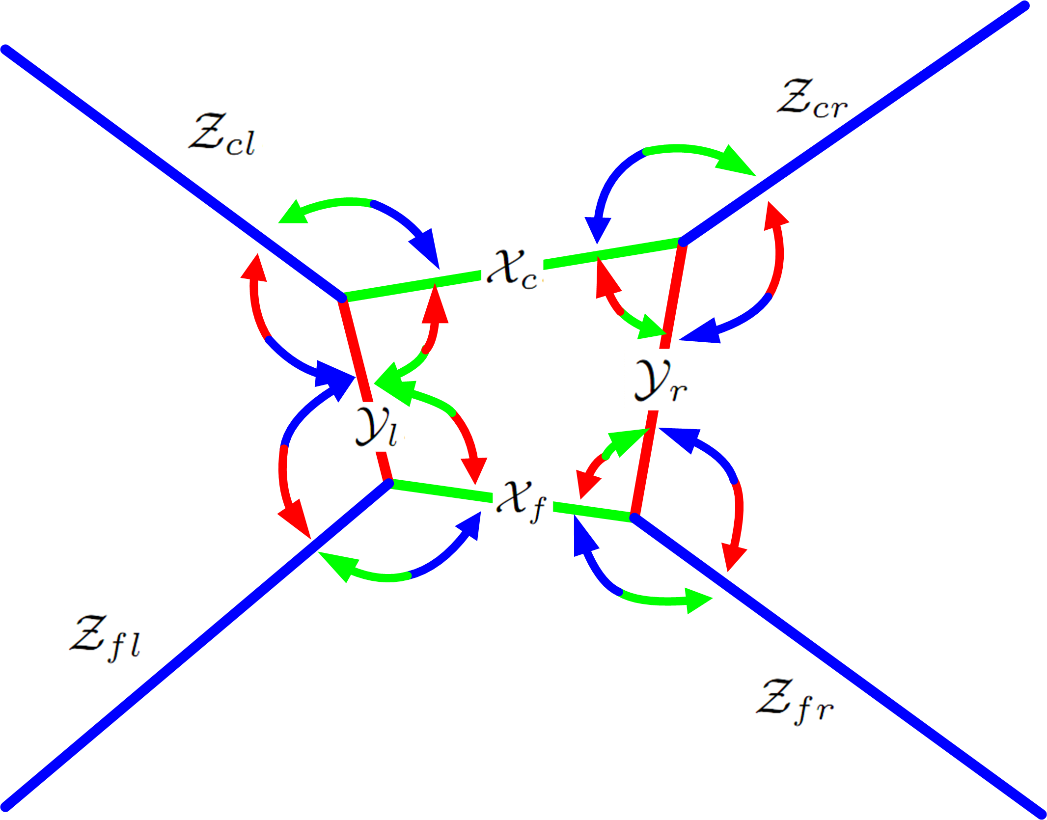
Figure 6: A sketch of the voting mechanism of ”4c”. Here we do not distinguish among status of $\mathcal{X}_{c}$, $\bar{\mathcal{X}}_{c}$, $\hat{\mathcal{X}}_{c}$, and $\bar{\mathcal{X}}_{c}\cup\hat{\mathcal{X}}_{c}$, we just use $\mathcal{X}_{c}$ for simple presentation. As shown, $\mathcal{Z}_{cl}$ is voted by $\mathcal{X}_{c}$ and $\mathcal{Y}_{l}$; $\mathcal{Z}_{cr}$ is voted by $\mathcal{X}_{c}$ and $\mathcal{Y}_{r}$; $\mathcal{Z}_{fl}$ is voted by $\mathcal{X}_{f}$ and $\mathcal{Y}_{l}$; $\mathcal{Z}_{fr}$ is voted by $\mathcal{X}_{f}$ and $\mathcal{Y}_{r}$; and $\mathcal{X}_{c}$ is voted by $\mathcal{Z}_{cl}$, $\mathcal{Z}_{cr}$, $\mathcal{Y}_{l}$, and $\mathcal{Y}_{r}$; $\mathcal{X}_{f}$ is voted by $\mathcal{Z}_{fl}$, $\mathcal{Z}_{fr}$, $\mathcal{Y}_{l}$, and $\mathcal{Y}_{r}$; $\mathcal{Y}_{l}$ is voted by $\mathcal{Z}_{cl}$, $\mathcal{Z}_{fl}$, $\mathcal{X}_{c}$, and $\mathcal{X}_{f}$; $\mathcal{Y}_{r}$ is voted by $\mathcal{Z}_{cr}$, $\mathcal{Z}_{fr}$, $\mathcal{X}_{c}$, and $\mathcal{X}_{f}$.

As known to peers, in indoor scenes with Manhattan assumption, each line segment points to one of three vanishing points. According to $\mathbf{R_{1}}$ that a supporting point exists because a box line blocks the extension of some line segment, if the box line are undetected for some reasons, however, the related groups of candidate supporting points are known, as well the related vanishing point, we can connect these candidate supporting points and the vanishing point to fit the missing box line, based on an assumption that one of the supporting points related to the undetected box line is in the groups of candidate supporting points. (As shown in Fig. 5)

As a result of fitting process, the line segment set $\mathcal{L}$ consists of two parts:

$$\mathcal{L}=\bar{\mathcal{L}}+\hat{\mathcal{L}},\quad\mathcal{L}=\{\mathcal{X},\mathcal{Y},\mathcal{Z}\},$$ (2)

where $\mathcal{\bar{L}}$ is the set of renewed line segments after the reclassifying and connecting, and $\hat{\mathcal{L}}$ is set of the added line segments of fitting.

4.4 Voting

To solve the fourth problem, according to $\mathbf{R_{2}}$ that any line segment cannot penetrate the boundary of the planes (the box lines), the line segments, whose endpoint is in related groups of candidate supporting points, can not penetrate the box line on the frame. Therefore, we can use those line segments to vote for the group of candidate box lines iteratively, to reduce the group. According to Fig. 4 that correspondences of the groups of candidate box lines and the related groups of supporting points, we use the line segments of the candidate supporting points to vote for the groups of candidate box lines. For example, for ”4c”, $\bar{\mathcal{X}}_{c}\cup\hat{\mathcal{X}}_{c}$ is voted by $\bar{\mathcal{Z}}_{cl}$, $\bar{\mathcal{Z}}_{cr}$, $\bar{\mathcal{Y}}_{l}$, and $\bar{\mathcal{Y}}_{r}$. Another vivid sketch of the voting mechanism of ”4c” is shown in Fig. 6, where we do not distinguish among statuses of $\mathcal{X}_{c}$, $\bar{\mathcal{X}}_{c}$, $\hat{\mathcal{X}}_{c}$, and $\bar{\mathcal{X}}_{c}\cup\hat{\mathcal{X}}_{c}$, we just use $\mathcal{X}_{c}$ for simple presentation.

To describe the detail voting process, we define two functions: a normalization function $\varphi(\cdot)$ and a reverse normalization function $\eta(\cdot)$ . We first initial the weight of each line segment in the groups of candidate box lines, the initial weight of candidate box line $l_{i}$ can be evaluated from two parts of length and angle:

$$\centering w_{\textrm{len}}=\psi_{(\textrm{len}(l_{i}))};~{}~{}~{}w_{\textrm{ang}}=\eta_{(\textrm{ang}(l_{i}))},\@add@centering$$ (3)

where $w_{\textrm{len}}$ denotes the weight of length of $l_{i}$; $w_{\textrm{ang}}$ denotes the weight of angle of $l_{i}$; $\textrm{len}(\cdot)$ denotes the length function at pixel level; $\textrm{ang}(\cdot)$ denotes the angle between $l_{i}$ and the line across the corresponding vanishing point and the middle point of $l_{i}$. For categories of ”4c”,”2hc”, and ”2vc”, the normalization or the reverse normalization implement on each subset (set, when ”1c”), where $l_{i}$ is. Further, initial weight of $l_{i}$ can be formulated as,

$$w_{i}^{0}=\xi_{\textrm{len}}\cdot w_{\textrm{len}}+\xi_{\textrm{ang}}\cdot w_{\textrm{ang}},$$ (4)

where $w_{i}^{0}$ is the initial weight of $l_{i}$, and $\xi_{\textrm{len}}+\xi_{\textrm{ang}}=1$. Besides, the line segments of $\mathcal{\hat{L}}$ is constructed by connecting vanishing points and candidate supporting points. Thus, calculating the length of those line segments is meaningless. Therefore, we ignore $l_{i}$ of $\mathcal{\hat{L}}$ when normalization of the part of length, and we set $\xi_{\textrm{len}}$ to 0 when calculating $w_{i}^{0}$ of $l_{i}\in\mathcal{\hat{L}}$.

After initializing each line segment in the groups of candidate box lines, for each group of candidate box lines, each candidate box line would be voted by those line segments, whose endpoint is in related groups of candidate supporting points . The voting weight for $l_{i}$ can be built from the weight of those line segments. Therefore, the voting weight can be formulated as,

$$v_{i}^{0}=\sum_{j}(-1)^{\textrm{label}}\cdot\lambda_{j}\cdot w_{j}^{0},$$ (5)

where $v_{i}^{0}$ is the voting weight of $l_{i}$, $w_{j}^{0}$ is the initial weight of $l_{j}$, one of those line segments, whose endpoint is in groups of candidate supporting points of $l_{i}$. For example, if $l_{i}\in\bar{\mathcal{Z}}_{cl}\cup\hat{\mathcal{Z}}_{cl}$, $l_{j}\in\bar{\mathcal{X}}_{c}\cup\bar{\mathcal{Y}}_{l}$. More details are shown in Fig. 7, where $l_{j}$ is voting for $l_{i}$, if $l_{i}$ and $l_{j}$ intersect, the label is equal to 1; otherwise, it is equal to 0. Further, by using the notations in Fig. 7, $\lambda_{j}$ is formulated as,

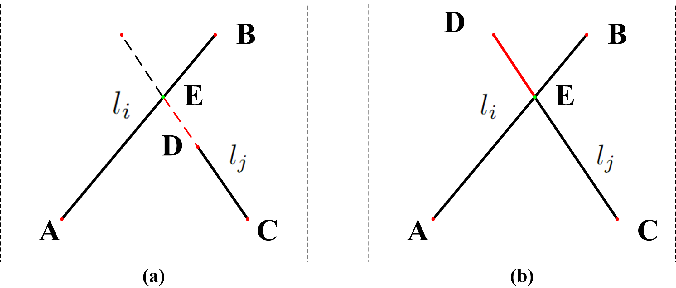
Figure 7: This is a sketch to describe line segment $l_{j}$ (i.e., $\overline{CD}$) voting for line segment $l_{i}$ (i.e., $\overline{AB}$). (a) $l_{i}$ and $l_{j}$ don’t intersect, yet the extension line of $l_{j}$ intersects with $l_{i}$ at $E$. (b) $l_{i}$ and $l_{j}$ intersect at $E$.

$$\begin{cases}\lambda=\psi(\frac{\textrm{min}(\textrm{len}(\overline{EC}),\textrm{len}(\overline{ED}))}{\textrm{len}(\overline{CD})}),&\textrm{label}=1\\ \lambda=\psi(\frac{\textrm{len}(\overline{CD})}{\textrm{len}(\overline{ED})}),&\textrm{label}=0\end{cases}$$ (6)

where the normalization implements on each subset (set, when ”1c”), where $l_{j}$ is. Consequently, after the first time of the loop, the weight of $l_{i}$ is as,

$$w_{i}^{1}=w_{i}^{0}+v_{i}^{0},$$ (7)

Further, the general weight function of $l_{i}$ can be formulated as,

$$w_{i}^{k+1}=w_{i}^{k}+v_{i}^{k},k\in N,$$ (8)

where $(k+1)$ is the time of the loop, $w_{i}^{k}$ is the weight of $l_{i}$ in the $(k+1)$-th time of the loop, and $v_{i}^{k}$ is the voting weight of $l_{i}$ in the $(k+1)$-th time.

At each time of the loop, we select the top $n=(5\sim 10)$ candidate box lines with highest weight in each subset (set, when ”1c”) or each group of candidate box lines. Until the selected candidate box lines maintain the same with those of the last time of the loop, we break the loop and save the final selected candidate box lines. After iteratively voting, $8\times n$, $5\times n$, $5\times n$, and $3\times n$ candidate box lines remain in ”4c”, ”2hc”, ”2vc”, and ”1c”, respectively.

5 Recovery the Frame

After line segment refinement, we start to recover the frame by fitting the corresponding frame model (Fig. 2) to the selected candidate box lines, with the cross ratio constraint and the depth constraint.

5.1 Candidate Frame Selection with Cross Ratio Constraint

In this subsection, groups of candidate box lines would be constrainted with cross ratio constraint, and built as candidate frames. According to the cross ratio invariance Mundy et al. [17] under Manhattan assumption, $\mathbf{R_{3}}$ that there is a cross ratio invariance among the box lines (the frame), guarantee the parallel and vertical relationships among the box lines. Unfortunately, because of the structure, there is not cross ratio invariance among the box lines of ”1c”. However, the problem has been solved by using the depth constraint in next subsection.

For categories of ”4c”, ”2hc”, and ”2vc”, cross ratio invariance is formulated as,

$$\begin{cases}\begin{cases}(x_{c},l_{xz}:x_{f},l_{xy})=(z_{cl},l_{xz}:z_{fl},l_{yz})=(z_{cr},l_{xz}:z_{fr},l_{yz})\\ (y_{r},l_{yz}:y_{l},l_{xy})=(z_{fl},l_{yz}:z_{fr},l_{xz})=(z_{cr},l_{yz}:z_{cl},l_{xz})\end{cases},&for~{}"4c"\\ (y_{l},l_{yz}:y_{r},l_{xy})=(z_{l},l_{yz}:z_{r},l_{xz}),&for~{}"2hc"\\ (x_{c},l_{xz}:x_{f},l_{xy})=(z_{c},l_{xz}:z_{f},l_{yz}).&for~{}"2vc"\end{cases}$$ (9)

Then, for ”4c”, the cross ratio constraint is as follows,

$$\begin{cases}\begin{cases}|2c_{(x,c,f)}-c_{(z,cl,fl)}-c_{(z,cr,fr)}|<\varepsilon\\ |2c_{(y,l,r)}-c_{(z,fl,fr)}-c_{(z,cl,cr)}|<\varepsilon\end{cases},&for~{}"4c"\\ |c_{(y,l,r)}-c_{(z,l,r)}|<\varepsilon,&for~{}"2hc"\\ |c_{(x,c,f)}-c_{(z,c,f)}|<\varepsilon,&for~{}"2vc"\end{cases}$$ (10)

where $\varepsilon\rightarrow 0^{+}$, and $c_{(x,c,f)}$ is a compact form of $(x_{c},l_{xz}:x_{f},l_{xy})$, the meanings of other denotations are similar.

For the categories of ”4c”,”2hc”, and ”2vc”, we traverse each group of candidate box lines, and put an element of each group into above inequations of cross ratio constraint. If related inequations have been satisfied, we save the set of satisfied candiate box lines and construct a candidate frame from the set; if not, ignore the unsatisfied set, and continue to test others. Until all sets of satisfied candidate box lines are selected, and all candidate frames are built from these sets, the traversing ends. After enforcing the cross ratio constraint, groups of candidate box lines are selected and built as candidate frames. (Fig. 1d)

5.2 Final Frame Selection by the Depth Constraint

To select the final frame from the candidate frames, we introduce $\mathbf{R_{4}}$ that the distance between the intersection of the box lines (corner of the frame) and the camera is the longest among the distances between the camera and other points nearby. First, the depth constraint or $\mathbf{R_{4}}$ is introduced by using the algorithm proposed by Criminisi et al. [4]. Their algorithm presents several calibration methods via vanishing points, and can calculate the relative location of 3D points. Second, we recover the 3D coordinates of the intersections of the box lines (corners), then, calculate the sum of distances between them and the 3D coordinate of camera optic center $\mathcal{O}$ (Fig. 8), for each category, which can be formulated as,

$$\begin{cases}\mathcal{S}=|\mathcal{\overline{OA}}|+|\overline{\mathcal{OB}}|+|\overline{\mathcal{OC}}|+|\overline{\mathcal{OD}}|,&for~{}"4c"\\ \mathcal{S}=|\mathcal{\overline{OA}}|+|\overline{\mathcal{OB}}|,&for~{}"2hc"~{}and~{}"2vc"\\ \mathcal{S}=|\mathcal{\overline{OA}}|.&for~{}"1c"\end{cases}$$ (11)

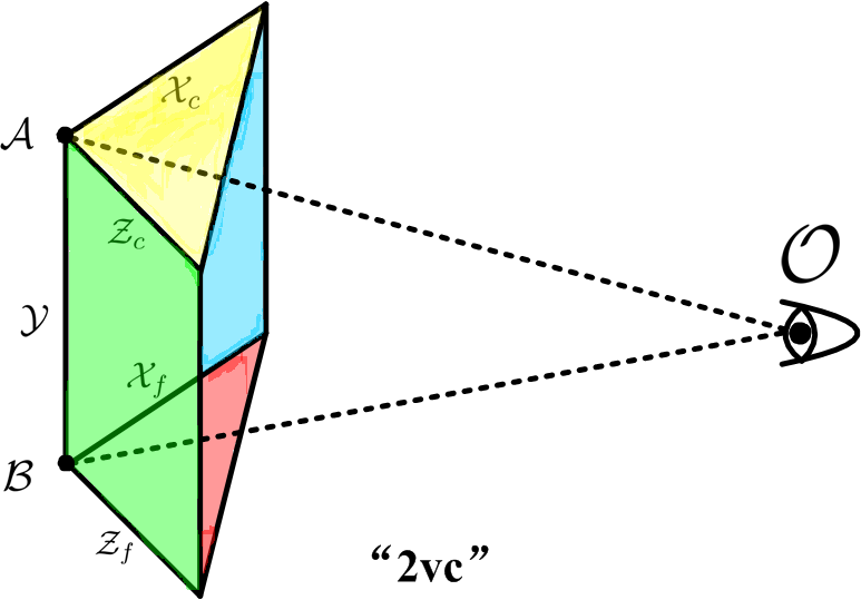
Figure 8: This is a sketch to illustrate the mechanism of depth constraint, taking ”2vc” as an example, where $\mathcal{A}$ and $\mathcal{B}$ are the intersections of box lines (corners), $\mathcal{O}$ is the camera optic.

where $\mathcal{A}$, $\mathcal{B}$, $\mathcal{C}$, and $\mathcal{D}$ are the intersections of box lines (corners). According to $\mathbf{R_{4}}$, $\mathcal{S}$ of the final frame should be the greatest among those of the candidate frames. Therefore, for each candidate frame, we calculate its $\mathcal{S}$ and select the frame with greatest $\mathcal{S}$ as the final frame.

6 Experiments & Results

All algorithms are evaluated on over 300 images of Hedau et al. [10] and some images collected from the internet. Those images include indoor scenes with difficulties from occlusions, illumination variations and weak object boundaries. All experiments are performed with MATLAB on a Windows system with a 3.2 GHz CPU and 2.0 GB RAM. We compare our method with the algorithms of Lee et al. [15] and Hedau et al. [15]. Besides, our initial line segments are based on Canny Edge Detector, as well as other algorithms.

We first qualitatively compare our method with the state-of-the-art approaches on indoor images with difficulties. Second, we quantitatively evaluate our algorithm on 150 indoor images, which consist of $50\times 3$ images with corners occluded in three different levels (Sec. 6.2). The three levels are denoted as ”0-occlusion”, ”1-occlusion”, and ”2-occlusion”. ”0-occlusion” means no occlusion appears on the corners. ”1-occlusion” represents there are little occlusions on the corners, while ”2-occlusion” stands for there are more occlusions on the corners. We use RMS error of corners, $C_{err}$, to evaluate the accuracy of the frame because if corners and vanishing points are known the frame is known as well. $C_{err}$ is the RMS error of corners location error compared with the ground-truth as a percentage of the image diagonal, which is formulated as,

$$\begin{cases}C_{err}=\frac{1}{n}\cdot\sum_{i=1}^{n}\left(\frac{|\overline{A^{i}A_{g}^{i}}|+|\overline{B^{i}B_{g}^{i}}|+|\overline{C^{i}C_{g}^{i}}|+|\overline{D^{i}D_{g}^{i}}|}{l^{i}}\right)^{2},&for~{}"4c"\\ C_{err}=\frac{1}{n}\cdot\sum_{i=1}^{n}\left(\frac{|\overline{A^{i}A_{g}^{i}}|+|\overline{B^{i}B_{g}^{i}}|}{l^{i}}\right)^{2},&for~{}"2hc"~{}and~{}"2vc"\\ C_{err}=\frac{1}{n}\cdot\sum_{i=1}^{n}\left(\frac{|\overline{A^{i}A_{g}^{i}}|}{l^{i}}\right)^{2},&for~{}"1c"\end{cases}$$ (12)

where $A$, $B$, $C$, and $D$ are corners of detected frame, $A_{g}$, $B_{g}$, $C_{g}$, and $D_{g}$ are the corners of ground-truth frame, $l$ is the image diagonal, $n$ is the number of the images in ”0-occlusion”, or ”1-occlusion”, or ”2-occlusion”, or all above three sets. The cases for ”4c”, ”2hc”, and ”1c” are similar. Ultimately, we compare the running speed with others on an image of $208\times 343$ resolution (Sec. 6.3).

6.1 Qualitative Evaluation

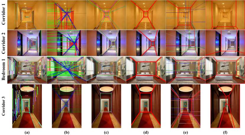
Figure 9: Comparisons on ”4c”. (a) is the initial line segments; (b) is our refined line segments; (c) is the candidate frames obtained with a cross ratio constraint; (d) is the final frame after introducing a depth constraint; (e) is the frames detected by the algorithm of Lee et al. [15] and the bold red frame is labeled as the best frame from their messy frames manually; (f) is the frame detected by the algorithm of Hedau et al. [10].

In this section, we qualitatively evaluate all algorithms on some typical images, where illumination varies, and there exist weak object boundaries and occlusions, as shown in Fig. 9, 10. We can see the initial line segments are messy, especially in Corridor-1,3, without the background it is hard to recognize the frame from these messy line segments. The refined line segments are much more regular, and there are tendencies of converging on the frame, especially the blue line segments show that. After enforcing the cross ratio constraint, we get the candidate frames, as shown at the third column of the figures. It can be seen that, besides the actual frame, there are many other frames appear, which happen to satisfy the cross ratio constraint. After enforcing the depth constraint, the final frame is selected, as shown at the fourth column, the frame is close to the ground-truth.

The algorithm of Lee et al. [15] is sensitive to occlusions, illumination variations, and weak object boundaries, especially in corridor series, TV-room, etc. Their algorithm can only work on images with regular line segments like Bedroom-1. Illumination variation is the Achilles’ heel of the algorithm by Hedau et al. [10], they cannot deal with the images of corridor, where illumination varies a lot. Yet, their algorithm is robust to occlusions to a certain extent via using occlusions as cues. Upon these figures, our method outperforms the state-of-the-art approaches of indoor frame recovery. The advantages of our method are derived mainly from the following strategies:

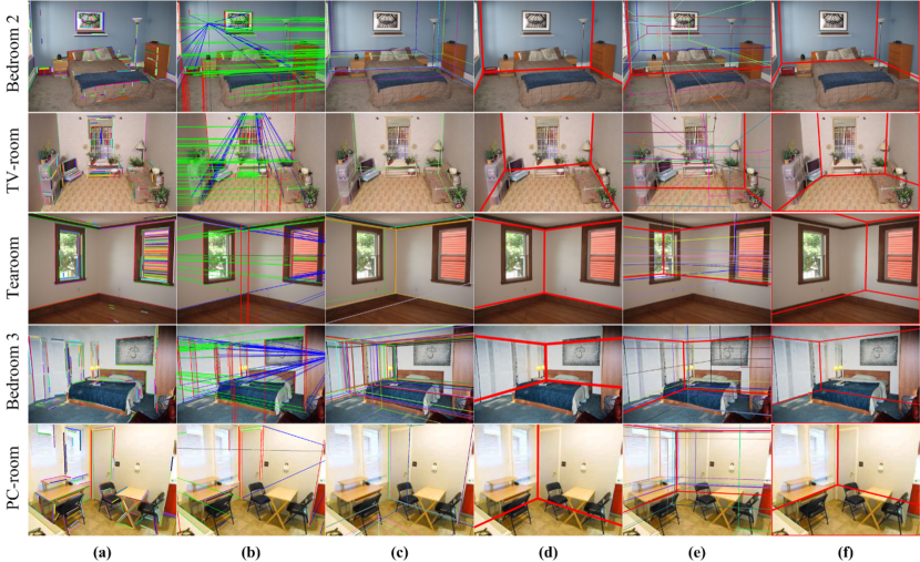
Figure 10: Comparisons on ”2hc”, ”2vc”, and ”1c”. The meaning of each column is the same as that in Fig. 9.

1. The procedures of refinement facilitate the recovery and selection of key line segments on the frame, where there are regions with illumination variations and occlusions. Without this line refinement strategy, the frames obtained by [15] and [10] are shapeless and twisted.

2. The cross ratio and depth constraints boost the construction and selection of superior frames. Compared with [10], which utilizes sampling and SVM ranking methods, our method can obtain better frames at a lower computational cost (Table 2).

6.2 Quantitative Evaluation

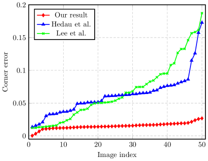
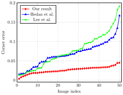
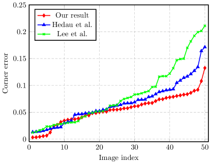
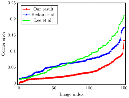
Figure 11: From up to down and left to right, the comparisons are on ”0-occlusion”, ”1-occlusion”, ”2-occlusion”, and ”0,1,2-occlusion”, respectively.

The depth constraint is helpless to a certain extent as the corners of the frame are occluded by furniture. Thus, we evaluate all algorithms on 150 images assigned to three levels in terms of the degree of occlusion on corners. Results are shown in Fig. 11 and Table 1, the $C_{err}$s of ours are $1.5\%$, $2.6\%$, and $5.5\%$ on ”0-occlusion”, ”1-occlusion”, and ”2-occlusion”, respectively. The gradients increase triply, which implies that our algorithm is not very robust to corner-occlusions. However, the refinement-process ensures the robustness of our algorithm to occlusions and illumination variations (Fig. 9b and Fig. 10b), the corner-occlusions only impact on selecting the final frame from candidate frames with the depth constraint. Without the depth constraint the corners of those candidate frames still distribute around the corners of ground-truth frame (Fig. 9c and Fig. 10c). Thus, no matter how occluded the corners are, with the two constraints and refined line segments, we can achieve an average $C_{err}$ of $3.2\%$ (Fig. 10-Bedroom-3).

Method	Lee et al.	Hedau et al.	Ours
”0-occlusion”	6.7%	6.2%	1.5%
”1-occlusion”	7.5%	6.8%	2.6%
”2-occlusion”	8.1%	6.7%	5.5%
”0,1,2-occlusion”	7.4%	6.6%	3.2%

Table 1: Corner error for frame estimation on ”0-occlusion”, ”1-occlusion”, and ”2-occlusion” with algorithms by Lee et al. [15], Hedau et al. [10], and ours, respectively. The $(i,j)$-th entry in the matrix represents the corner error of method $j$ on dataset $i$.

The $C_{err}$s of Hedau et al. [10] are $6.2\%$, $6.8\%$, and $6.7\%$ on ”0-occlusion”, ”1-occlusion”, and ”2-occlusion”, respectively, which are close to each other because they use the labeled occlusions as cues to fit the boundaries. It means that their method is robust to corner-occlusions to a certain extent. Yet their method is sensitive to illumination variations as a method based on geometric context and unrefined line segments. Therefore, their global $C_{err}$ ($6.6\%$) on ”0,1,2-occlusion” is greater than ours ($3.2\%$). The corner errors and gradients of Lee et al. [15] are greater than Hedau et al. [10] and ours, because they use line segments without refinement, which is sensitive to occlusions and illumination variations.

6.3 Running Time Evaluation

Algorithm	Processing time (s)
Lee et al.	32.61
Hedau et al.	505.79
Ours	5.26

Table 2: Running time comparison. The processing time of Hedau et al. [10] dose not contain the time of obtaining the geometric context, with the algorithm of Felzenszwalb et al. [5], via using their default parameters.

From the results illustrated in Table 2, our method is 6 times faster than [15] and 100 times faster than [10]. The algorithm by Hedau et al. [10] needs to manually label the furniture as cues to train a SVM ranking classifier. Lee et al. [15] needs to use a corner model of twelve statuses to fit the line segments and reason the integral frames. However, the solution space of our method is limited by voting of the line segment refinement and two constraints. Thus, we only spend 5.26 seconds during the whole process.

7 Discussion & Conclusion

7.1 Applications

The strategies of our algorithm can be widely used in building scenes satisfying the Manhattan Assumption, because our algorithm is based on the classified line segments derived from three orthogonal vanishing points, which can only be extracted from scenes satisfying the Manhattan Assumption.

For example, assuming that we would like to recover the frame of an object with strong structure characteristics (e.g., residential buildings, tables in a restaurant, and cabinet in a dim room, etc), it is inevitable to utilize extracted line segments. However, no matter how robust the algorithm of extracting line segments is, some key line segments are usually undetected for shadows, occlusions, and illumination, etc. It is easy to see that our fitting strategy could be used to address such problem. Moreover, after adding extra line segments, if the number of line segments is redundant for modeling, our voting strategy can eliminate those redundant line segments.

On the other hand, there are abundant clusters of parallel lines in the world, especially in building scenes. The cross ratio of the parallel line cluster in similar structure has the same value, and has affine invariance and perspective invariance. Thus, our cross ratio constraint can be used to restrict such model, or can be used to recover one line of the parallel line cluster.

7.2 Future work

As a line segment-based method, the line segment refinement of our algorithm relies on the accuracies of the three vanishing points. Simultaneously, the vanishing points are extracted from the line segments. Thus, an extension could be incorporating the refinement of vanishing points into the process of line segment refinement.

In addition, during the process of experiment, we find that it is still hard to achieve superior results when there are serious corner-occlusions with the help from depth. Therefore, another extension of our work could be integrating the texture surrounding the refined line segments into the framework of our algorithm.

7.3 Conclusion

In conclusion, we have presented a method to recover the frame of indoor scenes only from line segments, via using strategies derived from four significant natures of the box line and supporting point. We have shown that the refined line segments are improved a lot through line segment refinement. We also show that by restricting frame models with the cros ratio and depth constraints, the recovered frames outperform the ones of [15] and [10] in less running time. All conclusions are supported by the experimental results.

References

- [1] J. C. Bazin, Y. Seo, C. Demonceaux, P. Vasseur, K. Ikeuchi, I. Kweon, and M. Pollefeys. Globally optimal line clustering and vanishing point estimation in manhattan world. In CVPR, pages 638–645, 2012.
- [2] J. Biswas and M. M. Veloso. Depth camera based indoor mobile robot localization and navigation. In ICRA, pages 1697–1702, 2012.
- [3] J. Chu, A. GuoLu, L. Wang, C. Pan, and S. Xiang. Indoor frame recovering via line segments refinement and voting. In ICASSP, pages 1996–2000, 2013.
- [4] A. Criminisi, I. D. Reid, and A. Zisserman. Single view metrology. International Journal of Computer Vision, 40(2):123–148, 2000.
- [5] P. F. Felzenszwalb and D. P. Huttenlocher. Efficient graph-based image segmentation. International Journal of Computer Vision, 59(2):2004, 2004.
- [6] A. Flint, C. Mei, I. D. Reid, and D. W. Murray. Growing semantically meaningful models for visual slam. In CVPR, pages 467–474, 2010.
- [7] A. Flint, D. W. Murray, and I. Reid. Manhattan scene understanding using monocular, stereo, and 3d features. In ICCV, pages 2228–2235, 2011.
- [8] D. F. Fouhey, V. Delaitre, A. Gupta, A. A. Efros, I. Laptev, and J. Sivic. People watching: Human actions as a cue for single view geometry. In ECCV (5), pages 732–745, 2012.
- [9] F. Han and S. C. Zhu. Bottom-up/top-down image parsing with attribute grammar. IEEE Trans. Pattern Anal. Mach. Intell., 31(1):59–73, 2009.
- [10] V. Hedau, D. Hoiem, and D. A. Forsyth. Recovering the spatial layout of cluttered rooms. In ICCV, pages 1849–1856, 2009.
- [11] V. Hedau, D. Hoiem, and D. A. Forsyth. Thinking inside the box: Using appearance models and context based on room geometry. In ECCV (6), pages 224–237, 2010.
- [12] V. Hedau, D. Hoiem, and D. A. Forsyth. Recovering free space of indoor scenes from a single image. In CVPR, pages 2807–2814, 2012.
- [13] P. Kovesi. Phase congruency detects corners and edges. In DICTA, pages 309–318, 2003.
- [14] D. C. Lee, A. Gupta, M. Hebert, and T. Kanade. Estimating spatial layout of rooms using volumetric reasoning about objects and surfaces. In NIPS, pages 1288–1296, 2010.
- [15] D. C. Lee, M. Hebert, and T. Kanade. Geometric reasoning for single image structure recovery. In CVPR, pages 2136–2143, 2009.
- [16] X. Liu, O. Veksler, and J. Samarabandu. Graph cut with ordering constraints on labels and its applications. In CVPR, pages 1–8, 2008.
- [17] J. L. Mundy and A. Zisserman, editors. Geometric Invariance in Computer Vision. MIT Press, Cambridge, MA, USA, 1992.
- [18] L. D. Pero, J. Bowdish, D. Fried, B. Kermgard, E. Hartley, and K. Barnard. Bayesian geometric modeling of indoor scenes. In CVPR, pages 2719–2726, 2012.
- [19] L. D. Pero, J. Guan, E. Brau, J. Schlecht, and K. Barnard. Sampling bedrooms. In CVPR, pages 2009–2016, 2011.
- [20] A. Quattoni and A. Torralba. Recognizing indoor scenes. In CVPR, pages 413–420, 2009.
- [21] X. Ren, L. Bo, and D. Fox. Rgb-(d) scene labeling: Features and algorithms. In CVPR, pages 2759–2766, 2012.
- [22] C. Rother. A new approach for vanishing point detection in architectural environments. In In Proc. 11th British Machine Vision Conference, pages 382–391, 2000.
- [23] A. G. Schwing, T. Hazan, M. Pollefeys, and R. Urtasun. Efficient structured prediction for 3d indoor scene understanding. In CVPR, pages 2815–2822, 2012.
- [24] N. Silberman, D. Hoiem, P. Kohli, and R. Fergus. Indoor segmentation and support inference from rgbd images. In ECCV (5), pages 746–760, 2012.
- [25] J.-P. Tardif. Non-iterative approach for fast and accurate vanishing point detection. In ICCV, pages 1250–1257, 2009.
- [26] G. Tsai, C. Xu, J. Liu, and B. Kuipers. Real-time indoor scene understanding using bayesian filtering with motion cues. In ICCV, pages 121–128, 2011.
- [27] H. Wang, S. Gould, and D. Koller. Discriminative learning with latent variables for cluttered indoor scene understanding. In ECCV (2), pages 435–449, 2010.