Obtaining time-dependent multi-dimensional dividing surfaces using Lagrangian descriptors

Abstract

Dynamics between reactants and products are often mediated by a rate-determining barrier and an associated dividing surface leading to the transition state theory rate. This framework is challenged when the barrier is time-dependent because its motion can give rise to recrossings across the fixed dividing surface. A non-recrossing time-dependent dividing surface can neverthless be attached to the TS trajectory resulting in recrossing-free dynamics. We extend the formalism —contstructed using Lagrangian Descriptors— to systems with additional bath degrees of freedom. The propagation of reactant ensembles provides a numerical demonstration that our dividing surface is recrossing-free and leads to exact TST rates.

1 Introduction

The accuracy in the determination of reaction rates relies on the precision with which reactants and products can be distinguished in the underlying state space. Usually, the boundary between these regions contains an energetic saddle point in phase space to which an appropriate dividing surface (DS) can be attached. Transition state theory (TST) [1, 2, 3, 4, 5, 6, 7, 8, 9, 10, 11, 12, 13, 14, 15, 16, 17, 18] then provides a powerful basis for the qualitative and quantitative description of the reaction. The rate is obtained from the flux through the DS and it is exact if and only if the DS is free of recrossings. Advances in the determination of this fundamental quantity can impact a broad range of problems in atomic physics [19], solid state physics [20], cluster formation [21, 22], diffusion dynamics [23, 24], cosmology [25], celestial mechanics [26, 27], and Bose-Einstein condensates [28, 29, 30, 31, 32], to name a few.

In autonomous systems, the recrossing-free DS is attached to a normally hyperbolic invariant manifold that can be constructed using e. g. normal form expansions [33, 34, 35, 36, 37, 26, 38, 39, 40, 41]. The situation becomes fundamentally different if the system is time-dependent, e. g. if it is driven by an external field or subject to thermal noise. In one-dimensional time-dependent systems, a DS with the desired property is given by the transition state (TS) trajectory [42, 43, 44, 45, 46, 47, 48, 49, 50, 51] which is a unique trajectory bound to the vicinity of the saddle for all time.

In systems with dimension greater than one, the reacting particle can simply bypass the TS trajectory (point) by having a non-zero velocity perpendicular to the reaction coordinate. Thus one must attach a multi-dimensional surface to the TS trajectory that separates reactants and products. The use of perturbation theory in multi-dimensional cases provides both the TS trajectory and the associated geometry on which this dividing surface can be constructed. The challenge, addressed in this Letter, is how to obtain this multi-dimensional structure without perturbation theory. One possible approach lies in the use of the Lagrangian descriptor (LD) [52, 53] used recently by Hernandez and Craven [54, 55] to obtain the TS trajectory without resolving the DS at higher dimension. This alternate framework is necessary when there is no useful reference such as in barrierless reactions [49], and more generally to avoid the convergence issues that invariably plague a perturbation expansion far from the reference. In the case of field-induced ketene isomerization [55], the LD was computed across the entire phase space. It not only revealed the structure of the DS, but also coincided with the final state basins for each initial condition in phase space for both 1-dimensional and 2-dimensional representations. However, while the approach is formally applicable to arbitrary dimension, we have found that it is difficult to perform the minimization of the naive LD, even in dimensions as low as two.

The time-dependent Lagrangian descriptor dividing surface (LDDS), introduced in this Letter is the natural extension to $n$ dimensions for $n>1$. We freely choose $2n-2$ phase-space coordinates for which we fix the initial condidions, and use the LD approach to identify a corresponding trajectory, which we call an anchor trajectory. It is defined by the intersection of the stable and unstable manifolds of the time-dependent Hamiltonian [56, 57]. The TS trajectory is the anchor trajectory—which necessarily remains in the vicinity of the TS region for all past and future time—with the least vibrational motion orthogonal to the reactive degree of freedom. The LDDS is attached to the family of anchor trajectories and is necessarly $(2n-1)$-dimensional. In the special case of a one-dimensional system ($n=1$), the LDDS coincides with the moving DS on the TS trajectory [54].

2 Theory and Methods

2.1 Two-Dimensional Model System

We illustrate the construction of the LDDS by modeling the dynamics of a two-dimensional chemical reaction with stationary open reactant and product basins. Hamilton’s equation of motion propagates the particle according to a non-autonomous Hamiltonian in mass-weighted coordinates with potential

$$\begin{aligned} V(x,y,t)=\;&E_{\mathrm{b}}\,\exp\left(-a\left[x-\hat{x}\sin\left(\omega_{x}t\right)\right]^{2}\right)+\frac{\omega_{\mathrm{y}}^{2}}{2}\left[y-\frac{2}{\pi}\arctan\left(2x\right)\right]^{2}.\end{aligned}$$ (1)

Here, $E_{\mathrm{b}}$ is the height of a Gaussian barrier with width $a$ oscillating along the $x$ axis with frequency $\omega_{x}$ and amplitude $\hat{x}$, $\omega_{y}$ is the frequency of the harmonic potential in the $y$ direction, and the term $({2}/{\pi})\arctan\left(2x\right)$ is the minimum energy path whose form induces a nonlinear coupling between the two degrees of freedom. For simplicity, all variables are presented in dimensionless units, where the scales in energy (and $k_{\mathrm{B}}T$), length, and time are set according to half the maximum barrier height of the potential, twice the variance of the Gaussian distribution, and the inverse of the periodic frequency, respectively. In these units, the dimensionless parameters in Eq. (1) are set to $E_{\mathrm{b}}=2$, $a=1$, $\omega_{x}=\pi$, $\omega_{\mathrm{y}}=2$, and $\hat{x}=0.4$.

2.2 Using Lagrangian Descriptors to Obtain Dividing Surfaces

As the dividing surface between reactant and product basins is in general a high-dimensional hypersurface, the stable and unstable manifold itself become high-dimensional objects. In the context of TST, the Lagrangian descriptor (LD) at position $\boldsymbol{x}_{0}$, velocity $\boldsymbol{v}_{0}$, and time $t_{0}$, is defined as the integral [54, 49, 51],

$$\mathcal{L}(\boldsymbol{x}_{0},\boldsymbol{v}_{0},t_{0})=\int_{t_{0}-\tau}^{t_{0}+\tau}||\boldsymbol{v}(t)||\,\mathrm{d}t\,.$$ (2)

It is a measure of the arc length of the unique trajectory $\boldsymbol{x}(t)$ in forward and backward time over the time interval $[t_{0}-\tau;~{}t_{0}+\tau]$, and the parameter $\tau$ is chosen such that it covers the relevant time scale of the system [in this letter, we use $\tau=10$ corresponding to five periods of the oscillating barrier in Eq. (1)]. The importance of the LD (2) naturally results from the fact that the stable and unstable manifolds $\mathcal{W}_{\mathrm{s,u}}$ which are attached to the barrier top in phase space, correspond to the minimum of the forward (f: $t_{0}\leq t\leq t_{0}+\tau$) and backward (b: $t_{0}-\tau\leq t\leq t_{0}$) contributions to the LD,

$$\mathcal{W}_{\mathrm{s}}(\boldsymbol{x}_{0},\boldsymbol{v}_{0},t_{0}) =\operatorname*{arg\,min}~{}\mathcal{L}^{(\mathrm{f})}(\boldsymbol{x}_{0},\boldsymbol{v_{0}},t_{0}),$$ (3a)

$$\mathcal{W}_{\mathrm{u}}(\boldsymbol{x}_{0},\boldsymbol{v}_{0},t_{0}) =\operatorname*{arg\,min}~{}\mathcal{L}^{(\mathrm{b})}(\boldsymbol{x}_{0},\boldsymbol{v_{0}},t_{0}).$$ (3b)

Here, the function $\operatorname*{arg\,min}$ denotes the argument of the local minimum of the LD hypersurface close to the barrier top. In $n$ dimensions, we fix $2n-2$ variables freely (which would be least associated with the reactive degree of freedom) and perform the minimization in Eqs. (3). The intersection of these two manifolds

$$\mathcal{T}(x_{0},v_{0},t)\equiv\mathcal{W}_{\mathrm{s}}(x_{0},v_{0},t)\cap\mathcal{W}_{\mathrm{u}}(x_{0},v_{0},t),$$ (4)

is the $t=0$ value of the anchor trajectory to which a moving DS can be attached. The central result of this Letter is that the the family of these anchor trajectories $\mathcal{T}(t)$ carries the associated family of moving dividing surfaces that we call the Lagrangian descriptor dividing surface (LDDS), and that we show below to be a recrossing-free DS. The anchor surface $\mathcal{T}(t)$ is a $(2n-2)$-dimensional object embedded in the $2n$-dimensional phase space meaning in the special case of a one-dimensional system, this intersection is a single point, namely the position of the TS trajectory at given time [54].

The algorithm used to obtain $\mathcal{T}(t)$ can be explained by means of one of the insets in Fig. 1. These insets show the LD of an $x$-$v_{x}$-section for a certain time $t$ and fixed $y$ and $v_{y}$. The LD is calculated according to Eq. (2) by integrating trajectories with the respective initial conditions ($x,y,v_{x},v_{y},t$). They are obtained using a standard (symplectic) Velocity-Verlet integrator with a sufficiently small time-step to capture the time-dependence in the potential, Eq. (1), and to ensure convergence in the final positions and velocities. The structure of the stable and unstable manifold is identified through the local minima in the LD’s $x$-$v_{x}$-section. Their intersection yields the phase space coordinates, $x$ and $v_{x}$, of the point $\mathcal{T}(y,v_{y},t)$ to which the LDDS is attached. Repeating this procedure for an equidistant grid in the $y$-$v_{y}$ space (for a fixed time $t$) results in a mesh of points of the LDDS $\mathcal{T}(t)$. The smooth surfaces shown here are constructed through spline interpolation of this mesh.

3 Results

3.1 Trajectory Analysis

In Fig. 1 (center), we present a typical reactive trajectory (red solid line) undergoing a transition from the reactants ($x\to\infty$) to products ($x\to-\infty$). Because of the oscillating barrier in the two degree of freedom system (1), the trajectory shows several loops close to the barrier top. Its dominant motion is perpendicular to the reaction coordinate, but the trajectory also shows oscillations along the latter. Such nontrivial oscillations are a general feature of particles with an energy slightly above the barrier top. As a consequence, it is not generally possible to define a recrossing-free DS in the configuration space alone.

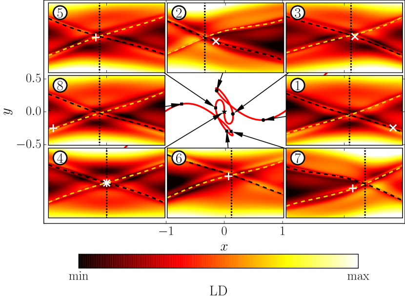
Figure 1: An illustrative trajectory of a reactive particle—in red in the center panel—undergoing multiple oscillations in the saddle region. Color maps of the LD surface at eight selected points ($x,v_{x}$)—marked with solid circles—along the reaction coordinate are shown at fixed values of the bath coordinates ($y,v_{y}$) displayed over the range $-0.8\leq x\leq 0.8$ on the horizontal axis and $-2.5\leq v_{x}\leq 2.5$ on the vertical axis. The stable (yellow) and unstable (black) manifolds are highlighted by dashed lines and the $x$-value of their intersection is marked by the vertical black dotted line. The position ($x,v_{x}$) of the particle on a given LD surface is shown by a white times ($\times$), asterisk ($\times+$), or plus ($+$) symbol, if the particle is located to the right, on, or to the left of the LDDS.

Although the particle’s dynamics is rather complicated near the barrier top, the reaction dynamics becomes clearer by focusing on the relative motion of the particle with respect to the time-dependent manifolds. In Fig. 1, phase space portraits of the LD are displayed for eight illustrative points along the selected trajectory. The stable (unstable) manifold corresponding to the minimum valleys of the LD according to Eq. (3) is shown as a black (yellow) dashed line. The time-dependent position $x^{\times}(y,v_{y})$ where they intersect is highlighted by a vertical, black dotted line. In the first three points, the particle is on the RHS of $x^{\times}(y,v_{y})$, crosses it at point 4, and then remains on the LHS of $x^{\times}(y,v_{y})$ for the last 4 point, as noted with the corresponding symbol defined in the caption. Each of the LD plots in the insets—labeled according to the corresponding point $1,\ldots,8$—shows an $x$-$v_{x}$-cut through phase space for the instantaneous values $y,v_{y}$ at the respective times $t$. In this and every other trajectory we have sampled, the particle crosses the corresponding $x^{\times}(y,v_{y})$ not more than once satisfying the recrossing-free criteria. For a single trajectory (that fixes $y$ and $v_{y}$ as the two remaining degrees of freedom in phase space and therefore leads to an effective one-dimensional system), the intersection of the manifolds (4) thus defines a recrossing-free DS that coincides with the TS trajectory of the effective one-dimensional system.

In the full phase space description of the two-dimensional system defined in Eq. (1), we can define a family of intersections $x^{\times}(y,v_{y})$ whose values and time-dependence vary depending on the two remaining bath coordinates (here $y$, $v_{y}$) according to Eq. (4). Indeed the union of these intersections is the time-dependent, two-dimensional anchor surface to which we attach the LDDS. The $\mathcal{T}(t)$ of Eq. (4) in the $x$, $y$, $v_{y}$ subspace is displayed in Fig. 2 (panel 7) at the time of the corresponding point in the trajectory. It is located near the saddle of the potential (1), shown as a contour-surface below, and exhibits a nontrivial curvature along all the axes. Note that the calculation of the associated time-dependent LDDS via the intersections of the manifolds in the $(x,v_{x})$ frame for a given $y$ and $v_{y}$ is exemplary, and the analogous approach using a different frame, such as $(y,v_{y})$, leads to the same result.

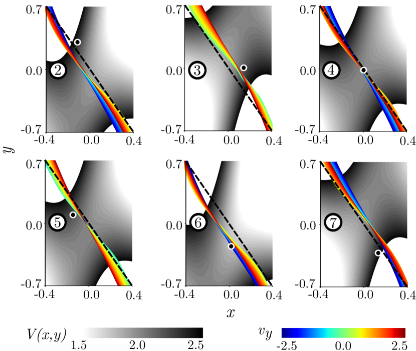
Figure 2: Snapshots of the corresponding to the insets 2–7 in Fig. 1. The $v_{y}$-dimension of each $\mathcal{T}(t)$ is encoded in the color bar on the right-hand side and the time-dependent saddle position is shown by the grayscale background. The black dot with white circle is the instantaneous position of the reactive particle whose trajectory is shown in Fig. 1. The dashed black line is shown to guide the eyes and as a reference to emphasize the surface’s motion.

A higher-dimensional representation of snapshots of the anchor surface for the same trajectory of Fig. 1 is shown in Fig. 2. The nontrivial motion of the curved anchor hypersurface over time emerges as one follows it in relation to the fixed black dashed line. The oscillation of the anchor surface is in phase with that of the barrier top, but its amplitude is about one order of magnitude smaller in configuration space. The recrossings of the LDDS attached to the anchor surface due to the loops in the particle’s trajectory of Fig. 1 are avoided by the motion and appropriate bending of the surface if the particle re-approaches the barrier region.

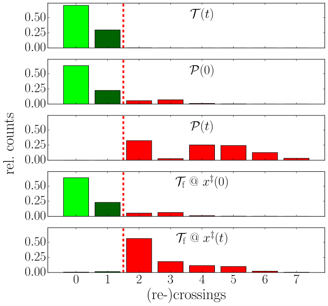
Figure 3: Comparison of the number of (re-)crossings obtained for the same ensemble and for different choices of DSs. The histograms are normalized to the whole particle number. Trajectories with zero and single crossings (green) lead to no error in the transition state estimate of the rate, while those with two and more crossings (red) lead to an overestimate of the rate. As shown in the top panel, the anchor surface $\mathcal{T}(t)$ to which the LDDS is attached does not lead to any recrossings and gives rise to a transition state theory rate that is exact.

3.2 Ensemble Analysis

We have, so far, demonstrated the recrossing-free nature of the LDDS attached to an anchor surface for a single trajectory. In the following, we extend this verification to an ensemble of trajectories. Specifically, 160 000 particles are initialized on an equidistant grid along the $x$-, $y$-, $v_{x}$-, and $v_{y}$-axes with 20 points along each axis. The grid is located close to the barrier top at $t=0$ and the grid size is chosen such that significant numbers of, both, reacting as well as nonreacting particles are observed during the time-evolution. For this ensemble, we compare in Fig. 3 different DSs with respect to their number of (re-)crossings. As can be seen in the first panel, the time-dependent LDDS attached to the anchor surface $\mathcal{T}(t)$ provides a recrossing-free DS for the whole ensemble of particles. For comparison, we introduce additional DSs for which we again calculate the number of recrossings yielding the other panels in Fig. 3. A naive way to construct a DS would be a planar surface perpendicular to the minimum energy path and attached to the time-dependently moving barrier top $x^{\ddagger}(t)$ which we refer to as $\mathcal{P}(t)$. In a second case, called $\mathcal{P}(0)$, we keep this planar surface fixed at the saddle’s initial position $x^{\ddagger}(0)$. The last two histograms are calculated using the LDDS for the fixed, time-independent potential $V(x,~{}y,~{}0)$ of Eq. (1). The resulting time-independent DS is either fixed at the saddle’s initial position [$\mathcal{T}_{\mathrm{f}}~{}@~{}x^{\ddagger}(0)$] or periodically moving with the top of the barrier [$\mathcal{T}_{\mathrm{f}}~{}@~{}x^{\ddagger}(t)$]. As Fig. 3 shows, the LDDS is the only choice for which either no or only single crossings occur while two and more crossings do not occur. By contrast, all the other choices of DSs exhibit several recrossings and will therefore lead to overestimates in the corresponding rates.

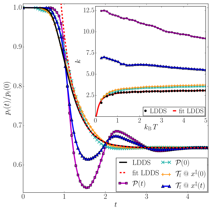
Figure 4: Black line: relative number of reactants $p_{\mathrm{r}}$ over time for an initial thermal ensemble ($k_{\mathrm{B}}T=5.13$) of reactant particles crossing the LDDS. The corresponding curve (red dashed line) yields a rate of $k=3.03$ via an exponential fit. The other curves show the number of reactants for those surfaces mentioned in Fig. 3. The inset shows the temperature dependence of the rates $k$ obtained from the fit (6). The rates obtained from the LDDS yields a high-temperature rate of $k_{\infty}=3.14$. See text for further description.

Finally, we regard a thermal ensemble of $10^{6}$ particles in the reactant well with the density distribution

$$\rho(\boldsymbol{x},\boldsymbol{v})=\rho_{\mathrm{therm}}\,\delta(x+2)\,\Theta(v_{x})\,,$$ (5)

where $\rho_{\mathrm{therm}}$ is a Boltzmann-distribution, $\delta$ is the Dirac-delta function and $\Theta$ the Heaviside step function. The corresponding time-evolution of the reactant population $p_{\mathrm{r}}(t)$ is shown in Fig. 4. The decay corresponding to the LDDS is the only strictly monotonic one. Both of the time-independent DSs exhibit a modulation of the reactant population with a very small but nonvanishing amplitude. When fixed DSs are attached to the barrier top, $x^{\ddagger}(t)$, the oscillations are huge. Each increase in the number of reactants is due to recrossings through the respective surface. Note that for $t\rightarrow\infty$, the reactant population for all DSs is the same, as the particles have fallen down from the barrier either in the reactant or in the product basin and their classification is independent of the choice of the dividing surface, as long as it is located sufficiently close to the saddle.

The red dashed line in Fig. 4 shows an exponential fit

$$p_{\mathrm{r}}(t)=p_{\mathrm{r,0}}\,\mathrm{e}^{-kt}+c$$ (6)

to the long-time decay of the reactant population with fit coefficients $p_{\mathrm{r,0}},k,c$ from which we extract the reaction rate $k$. The respective rates obtained for the different DSs at various temperatures $k_{\mathrm{B}}T$ are shown in the inset of Fig. 4. Rates obtained from the LDDS are the smallest throughout as should be expected from a recrossing-free DS. The time-independent $\mathcal{P}(0)$ and $\mathcal{T}_{\mathrm{f}}(0)$ yield slightly higher rates while the rates obtained from the DSs attached to the barrier top [$\mathcal{P}(t)$ and $\mathcal{T}_{\mathrm{f}}(t)$] overestimate the rates by a factor of 2 to 5 due to recrossings. In addition, the LDDS rates exhibit a temperature dependence according to Arrhenius’ rate equation (see red fit curve in the inset of Fig. 4),

$$k(k_{\mathrm{B}}T)=k_{\infty}\,\exp\left(-\frac{\Delta E_{\mathrm{eff}}}{k_{\mathrm{B}}T}\right),$$ (7)

where $\Delta E_{\mathrm{eff}}=0.135$ is the effective height of the potential and $k_{\infty}=3.14$ is the high-temperature limit of the rate. The effective barrier height is significantly lower than the spread of barrier heights between 1.70 to 2.00 at the naive saddle point. The fact that $\Delta E_{\mathrm{eff}}$ is not higher than these barrier heights is a good consistency check. It is lower in energy because the driving of the system maintains the effective reactant population in an activated state energetically higher than the naive reactant population near the minimum of the potential.

4 Conclusion

In this Letter, we have developed and verified the explicit construction of the time-dependent LDDS for multidimensional systems as a recrossing-free dividing surface. It reduces to the well-known TS trajectory [42] formalism in the one-dimensional limit.

The central result of this Letter is thus the justification and validation of a generalization of the LDDS method whose underlying minimization converges even in higher dimensions. Specifically, the construction is realizable because the LD (2) remains a scalar quantity regardless of the phase space dimension. The construction also results in a global DS, i. e. the recrossing-free property does not only hold close to the barrier top but for the complete hypersurface in full phase space. The method thus positions us to resolve the dividing surface (and associated reaction rates) in time-dependent molecular reactions [58, 59, 60, 61, 62, 63], and perhaps also spintronic devices [64, 65] driven by tailored external fields or thermal noise.

References

References

- [1] K. S. Pitzer, F. T. Smith, H. Eyring, The Transition State, Special Publ., Chemical Society, London, 1962.
- [2] P. Pechukas, Transition state theory, Annu. Rev. Phys. Chem. 32 (1981) 159–177.
- [3] B. C. Garrett, D. G. Truhlar, Generalized transition state theory, J. Phys. Chem. 83 (1979) 1052–1079.
- [4] D. G. Truhlar, A. D. Issacson, B. C. Garrett, Theory of Chemical Reaction Dynamics, Vol. 4, CRC Press, Boca Raton, FL, 1985, pp. 65–137.
- [5] J. T. Hynes, Chemical reaction dynamics in solution, Annu. Rev. Phys. Chem. 36 (1985) 573–597.
- [6] B. J. Berne, M. Borkovec, J. E. Straub, Classical and modern methods in reaction rate theory, J. Phys. Chem. 92 (1988) 3711–3725.
- [7] A. Nitzan, Activated rate processes in condensed phases: The kramers theory revisited, Adv. Chem. Phys. 70 (1988) 489–555.
-
[8]
P. Hänggi, P. Talkner, M. Borkovec,
Reaction-rate
theory: Fifty years after kramers, Rev. Mod. Phys. 62 (1990) 251–341, and
references therein.
URL http://link.aps.org/doi/10.1103/RevModPhys.62.251 - [9] G. A. Natanson, B. C. Garrett, T. N. Truong, T. Joseph, D. G. Truhlar, The definition of reaction coordinates for reaction-path dynamics, J. Chem. Phys. 94 (1991) 7875–7892.
- [10] D. G. Truhlar, B. C. Garrett, S. J. Klippenstein, Current status of transition-state theory, J. Phys. Chem. 100 (1996) 12771–12800.
- [11] D. G. Truhlar, B. C. Garrett, Multidimensional transition state theory and the validity of Grote-Hynes theory, J. Phys. Chem. B 104 (5) (2000) 1069–1072.
- [12] T. Komatsuzaki, R. S. Berry, Dynamical hierarchy in transition states: Why and how does a system climb over the mountain?, Proc. Natl. Acad. Sci. U.S.A. 98 (14) (2001) 7666–7671.
- [13] E. Pollak, P. Talkner, Reaction rate theory: What it was, where it is today, and where is it going?, Chaos 15 (2005) 026116.
- [14] H. Waalkens, R. Schubert, S. Wiggins, Wigner’s dynamical transition state theory in phase space: classical and quantum, Nonlinearity 21 (1) (2008) R1.
- [15] T. Bartsch, J. M. Moix, R. Hernandez, S. Kawai, T. Uzer, Time-dependent transition state theory, Adv. Chem. Phys. 140 (2008) 191–238.
- [16] S. Kawai, T. Komatsuzaki, Robust existence of a reaction boundary to separate the fate of a chemical reaction, Phys. Rev. Lett. 105 (2010) 048304.
- [17] R. Hernandez, T. Bartsch, T. Uzer, Transition state theory in liquids beyond planar dividing surfaces, Chem. Phys. 370 (2010) 270–276.
- [18] O. Sharia, G. Henkelman, Analytic dynamical corrections to transition state theory, New J. Phys. 18 (1) (2016) 013023.
- [19] C. Jaffé, D. Farrelly, T. Uzer, Transition state theory without time-reversal symmetry: Chaotic ionization of the hydrogen atom, Phys. Rev. Lett. 84 (2000) 610–614.
- [20] G. Jacucci, M. Toller, G. DeLorenzi, C. P. Flynn, Rate Theory, Return Jump Catastrophes, and the Center Manifold, Phys. Rev. Lett. 52 (1984) 295. doi:10.1103/PhysRevLett.52.295.
- [21] T. Komatsuzaki, R. S. Berry, Regularity in chaotic reaction paths. I. , J. Chem. Phys. 110 (18) (1999) 9160–9173.
- [22] T. Komatsuzaki, R. S. Berry, Chemical reaction dynamics: Many-body chaos and regularity, Adv. Chem. Phys. 123 (2002) 79–152.
- [23] M. Toller, G. Jacucci, G. DeLorenzi, C. P. Flynn, Theory of classical diffusion jumps in solids, Phys. Rev. B 32 (1985) 2082.
- [24] A. F. Voter, F. Montalenti, T. C. Germann, Extending the time scale in atomistic simulations of materials, Annu. Rev. Mater. Res. 32 (2002) 321–346.
- [25] H. P. de Oliveira, A. M. Ozorio de Almeida, I. Damiõ Soares, E. V. Tonini, Homoclinic chaos in the dynamics of a general Bianchi type-IX model, Phys. Rev. D 65 (8) (2002) 083511/1–9.
- [26] C. Jaffé, S. D. Ross, M. W. Lo, J. Marsden, D. Farrelly, T. Uzer, Statistical theory of asteroid escape rates, Phys. Rev. Lett. 89 (1) (2002) 011101. doi:10.1103/PhysRevLett.89.011101.
- [27] H. Waalkens, A. Burbanks, S. Wiggins, Escape from planetary neighborhoods, Mon. Not. R. Astron. Soc. 361 (2005) 763.
- [28] C. Huepe, S. Métens, G. Dewel, P. Borckmans, M. E. Brachet, Decay rates in attractive Bose-Einstein condensates, Phys. Rev. Lett. 82 (1999) 1616. doi:10.1103/PhysRevLett.82.1616.
- [29] C. Huepe, L. S. Tuckerman, S. Métens, M. E. Brachet, Stability and decay rates of nonisotropic attractive Bose-Einstein condensates, Phys. Rev. A 68 (2003) 023609. doi:10.1103/PhysRevA.68.023609.
- [30] A. Junginger, J. Main, G. Wunner, M. Dorwarth, Transition state theory for wave packet dynamics. I. Thermal decay in metastable Schrödinger systems, J. Phys. A: Math. Theor. 45 (2012) 155201.
- [31] A. Junginger, M. Dorwarth, J. Main, G. Wunner, Transition state theory for wave packet dynamics. II. Thermal decay of Bose-Einstein condensates with long-range interaction, J. Phys. A: Math. Theor. 45 (2012) 155202.
- [32] A. Junginger, M. Kreibich, J. Main, G. Wunner, Transition states and thermal collapse of dipolar Bose-Einstein condensates, Phys. Rev. A 88 (2013) 043617.
- [33] E. Pollak, P. Pechukas, Transition states, trapped trajectories, and classical bound states embedded in the continuum, J. Chem. Phys. 69 (1978) 1218–1226.
- [34] P. Pechukas, E. Pollak, Classical transition state theory is exact if the transition state is unique, J. Chem. Phys. 71 (1979) 2062–2068.
- [35] R. Hernandez, W. H. Miller, Semiclassical transition state theory. A new perspective, Chem. Phys. Lett. 214 (1993) 129–136.
- [36] R. Hernandez, A combined use of perturbation theory and diagonalization: Application to bound energy levels and semiclassical rate theory, J. Chem. Phys. 101 (1994) 9534–9547.
- [37] T. Uzer, C. Jaffé, J. Palacián, P. Yanguas, S. Wiggins, The geometry of reaction dynamics, Nonlinearity 15 (4) (2002) 957–992.
- [38] H. Teramoto, M. Toda, T. Komatsuzaki, Dynamical switching of a reaction coordinate to carry the system through to a different product state at high energies, Phys. Rev. Lett. 106 (2011) 054101(1)–054101(4).
- [39] C.-B. Li, A. Shoujiguchi, M. Toda, T. Komatsuzaki, Definability of no-return transition states in the high-energy regime above the reaction threshold, Phys. Rev. Lett. 97 (2006) 028302(1)–028302(4).
- [40] H. Waalkens, S. Wiggins, Direct construction of a dividing surface of minimal flux for multi-degree-of-freedom systems that cannot be recrossed, J. Phys. A 37 (35) (2004) L435–L445.
- [41] U. Çiftçi, H. Waalkens, Reaction dynamics through kinetic transition states, Phys. Rev. Lett. 110 (2013) 233201(1)–233201(4).
- [42] T. Bartsch, R. Hernandez, T. Uzer, Transition state in a noisy environment, Phys. Rev. Lett. 95 (2005) 058301(1)–058301(4).
- [43] T. Bartsch, T. Uzer, R. Hernandez, Stochastic transition states: Reaction geometry amidst noise, J. Chem. Phys. 123 (2005) 204102(1)–204102(14).
- [44] T. Bartsch, T. Uzer, J. M. Moix, R. Hernandez, Identifying reactive trajectories using a moving transition state, J. Chem. Phys. 124 (2006) 244310(01)–244310(13).
- [45] S. Kawai, T. Komatsuzaki, Dynamic pathways to mediate reactions buried in thermal fluctuations. i. time-dependent normal form theory for multidimensional langevin equation, J. Chem. Phys. 131 (2009) 224505(1)–224505(11).
- [46] G. T. Craven, T. Bartsch, R. Hernandez, Persistence of transition state structure in chemical reactions driven by fields oscillating in time, Phys. Rev. E 89 (2014) 040801(1)–040801(5).
- [47] G. T. Craven, T. Bartsch, R. Hernandez, Communication: Transition state trajectory stability determines barrier crossing rates in chemical reactions induced by time-dependent oscillating fields, J. Chem. Phys. 141 (2014) 041106(1)–041106(5).
- [48] G. T. Craven, T. Bartsch, R. Hernandez, Chemical reactions induced by oscillating external fields in weak thermal environments, J. Chem. Phys. 142 (2015) 1–13.
- [49] A. Junginger, R. Hernandez, Uncovering the geometry of barrierless reactions using Lagrangian descriptors, J. Phys. Chem. B 120 (2016) 1720.
- [50] A. Junginger, G. T. Craven, T. Bartsch, F. Revuelta, F. Borondo, R. M. Benito, R. Hernandez, Transition state geometry of driven chemical reactions on time-dependent double-well potentials, Phys. Chem. Chem. Phys. 18 (2016) 30270.
- [51] A. Junginger, R. Hernandez, Lagrangian descriptors in dissipative systems, Phys. Chem. Chem. Phys. 18 (2016) 30282.
- [52] C. Mendoza, A. M. Mancho, Hidden geometry of ocean flows, Phys. Rev. Lett. 105 (2010) 038501.
- [53] A. M. Mancho, S. Wiggins, J. Curbelo, C. Mendoza, Lagrangian descriptors: A method for revealing phase space structures of general time dependent dynamical systems, Commun. Nonlinear Sci. Numer. Simul. 18 (12) (2013) 3530 – 3557.
- [54] G. T. Craven, R. Hernandez, Lagrangian descriptors of thermalized transition states on time-varying energy surfaces, Phys. Rev. Lett. 115 (2015) 148301.
- [55] G. T. Craven, R. Hernandez, Deconstructing field-induced ketene isomerization through Lagrangian descriptors, Phys. Chem. Chem. Phys. 18 (2016) 4008–4018.
- [56] A. J. Lichtenberg, M. A. Liebermann, Regular and Stochastic Motion, Springer, New York, 1982.
- [57] E. Ott, Chaos in dynamical systems, second edition Edition, Cambridge University Press, Cambridge, 2002.
- [58] K. Yamanouchi, The next frontier, Science 295 (5560) (2002) 1659–1660.
- [59] B. J. Sussman, D. Townsend, M. Y. Ivanov, A. Stolow, Dynamic Stark control of photochemical processes, Science 314 (5797) (2006) 278–281.
- [60] S. Kawai, T. Komatsuzaki, Quantum reaction boundary to mediate reactions in laser fields, J. Chem. Phys. 134 (2) (2011) 024317.
- [61] A. Sethi, S. Keshavamurthy, Local phase space control and interplay of classical and quantum effects in dissociation of a driven Morse oscillator, Phys. Rev. A 79 (2009) 033416.
- [62] S. Patra, S. Keshavamurthy, Classical-quantum correspondence in a model for conformational dynamics: Connecting phase space reactive islands with rare events sampling, Chem. Phys. Lett. 634 (2015) 1–10.
- [63] F. Revuelta, R. Chacón, F. Borondo, Towards ac-induced optimum control of dynamical localization, Europhys. Lett. 110 (4) (2015) 40007.
- [64] T. Taniguchi, Y. Utsumi, H. Imamura, Thermally activated switching rate of a nanomagnet in the presence of spin torque, Phys. Rev. B 88 (2013) 214414.
- [65] D. M. Apalkov, P. B. Visscher, Spin-torque switching: Fokker-Planck rate calculation, Phys. Rev. B 72 (2005) 180405(R).
- [66] P. Ramachandran, G. Varoquaux, Mayavi: 3D Visualization of Scientific Data, Computing in Science & Engineering 13 (2) (2011) 40–51.