Towards a formal definition of static and dynamic electronic correlations

Abstract

Some of the most spectacular failures of density-functional and Hartree-Fock theories are related to an incorrect description of the so-called static electron correlation. Motivated by recent progress on the N-representability problem of the one-body density matrix for pure states, we propose a way to quantify the static contribution to the electronic correlation. By studying several molecular systems we show that our proposal correlates well with our intuition of static and dynamic electron correlation. Our results bring out the paramount importance of the occupancy of the highest occupied natural spin-orbital in such quantification.

I Introduction

The concept of correlation and more precisely the idea of correlation energy are central in quantum chemistry. Indeed, the electron-correlation problem (or how the dynamics of each electron is affected by the others) is perhaps the single largest source of error in quantum-chemical computations Tew, Klopper, and Helgaker (2007). The success of Hartree-Fock theory in providing a workable upper bound for the ground-state energy is largely due to the fact that a single Slater determinant is usually the simplest wave function having the correct symmetry properties for a system of fermions. Since the description of interacting fermionic systems requires multi-determinantal reference wave functions, the correlation energy is commonly defined as the difference between the exact ground-state and the Hartree-Fock energy Wigner (1934); Löwdin (1955). Beyond Hartree-Fock theory, numerous other methods (such as configuration interaction or coupled-cluster theory) aim at reconstructing the part of the energy missing from a description based on a single-determinantal wave function. Indeed, one common indicator of the accuracy of a model is, by and large, the percentage of the correlation energy it is able to recover.

For small molecules, variational methods based on configuration interaction techniques describe well electronic correlations. However, due to their extreme computational cost, configuration-interaction wavefunctions are noteworthily difficult to evaluate for larger systems. Among other procedures at hand, the correlation can be treated efficiently by applying a Jastrow correlation term to an antisymmetrized wave function (e.g. a single Slater determinant or an antisymmetrized geminal power) within quantum Monte Carlo methods Casula and Sorella (2003); Casula, Attaccalite, and Sorella (2004). The so-called Jastrow antisymmetric geminal ansatz accounts for inter-pair interactions and multiple resonance structures, maintaining a polynomial scaling cost, comparable to that of the simpler Jastrow single determinant approach. Highly correlated systems, as diradical molecules (the orthogonally twisted ethylene C₂H₄ and the methylene CH₂, for example) and bond stretching in H₂O, C₂ and N₂, are well described by such a method Zen et al. (2014); Neuscamman (2013).

In recent years a considerable effort has been devoted to characterize the correlation of a quantum system in terms of more meaningful quantities, such as the Slater rank for two-electron systems Schliemann et al. (2001); Plastino, Manzano, and Dehesa (2009), the entanglement classification for the three-fermion case Sárosi and Lévay (2014), the squared Frobenius norm of the cumulant part of the two-particle reduced density matrix Juhász and Mazziotti (2006) or the comparison with uncorrelated states Gottlieb and Mauser (2005). Along with Christian Schilling, we have recently stressed the importance of the energy gap in the understanding of the electronic correlations Benavides-Riveros et al. (2017). Notwithstanding, these measures do not draw a distinction between qualitatively different kinds of electronic correlations. In quantum chemistry, for instance, it is customary to distinguish between static (or nondynamic) and dynamic correlations. The former corresponds to configurations which are nearly degenerate with respect to the reference Slater determinant (if any), whilst the latter arises from the need of mixing the Hartree-Fock state with higher-order excited states Becke (2013); Ziesche et al. (1997). Heuristically, one usually states that in systems with (strong) static correlation the wavefunction differs qualitatively from the reference Slater determinant, while strong dynamic correlation implies a wavefunction including a large number of excited determinants, all with comparable, small occupations. Some of the most spectacular failures of the Hartree-Fock theory and density functional theory (with standard exchange-correlation functionals) are related to an incorrect description of static correlation Cohen, Mori-Sánchez, and Yang (2008a).

It is commonly believed that, to a large extent, both static and dynamic contributions should be included in the global computation of the electronic correlation. Yet there are few systems for which one can distinguish unambiguously between these two types of correlations. For instance, the ground state of helium has no excited electronic states nearby, leading therefore to the absence of static correlation. In the dissociation limit of H₂ a state with fractional occupations arises Cohen, Mori-Sánchez, and Yang (2008b) and the correlation is purely static. According to Hollett and Gill Hollett and Gill (2011), static correlation comes in two “flavors”: one that can be captured by breaking the spin symmetry of the Hartree-Fock wave function (like in stretched H₂) and another that cannot. The measures of correlation proposed so far purport to include both static and dynamic correlations, although in an uncontrolled manner Hollett, Hosseini, and Menzies (2016).

For pure quantum states, global structural features of the wave function can be abstracted from local information alone. Multiparticle entanglement, for instance, can be completely classified with the more accesible one-particle picture Walter et al. (2013). Such a characterization is addressed by a finite set of linear inequalities satisfied by the eigenvalues of the single-particle states Sawicki, Walter, and Kuś (2013). Furthermore, by using the two-particle density matrix and its deviation from idempotency, it is possible to propose a criterion to distinguish static from dynamic correlation, which for two-fermion systems only requires the occupancies of the natural orbitals Ramos-Cordoba, Salvador, and Matito (2016). Needless to say, grasping global information of a many-body quantum system by tackling only one-particle information is quite remarkable, mainly because in this way a linear number of degrees of freedom is required.

Recent progress on the N-representability problem of the one-body reduced density matrix for pure states provides an extension of the well-known Pauli exclusion principle Klyachko (2006). This extension is important because it provides stringent constraints beyond those from the Pauli principle, which can be used, among others, to improve reduced-density-matrix functional theories Theophilou et al. (2015); Mazziotti (2016); DePrince (2016). Our main aim in this paper is to employ the generalized Pauli exclusion principle to establish a general criterion to distinguish static and dynamic contributions to the electronic correlation in fermionic systems.

The paper is organized as follows. For completeness, Section II summarizes the key aspects of the so-called generalized Pauli exclusion principle and its potential relevance for quantum chemistry. In Section III we discuss a Shull-Löwdin-type functional for three-fermion systems, which can be constructed by using the pertinent generalized Pauli constraints along with the spin symmetries. Since this functional depends only on the occupation numbers, it is possible to distinguish the correlation degree of the so-called Borland-Dennis setting (with an underlining six-dimensional one-particle Hilbert space) by using one-particle information alone. In Section IV we discuss a formal way to distinguish static from dynamic correlation. Section V is devoted to investigate the static and dynamic electronic correlation in molecular systems. We compare our results with the well-known von-Neumann entanglement entropy. The paper ends with a conclusion and an appendix.

II The generalization of the Pauli principle

In a groundbreaking work, aimed at solving the quantum marginal problem for pure states, Alexander Klyachko generalized the Pauli exclusion principle and provided a set of constraints on the natural occupation numbers, stronger than the Pauli principle Klyachko (2006). Although rudimentary schemes to construct such constraints were, to some extent, routine in quantum-chemistry literature Müller (1999), it was not only with the work of Klyachko that this rich structure could be decrypted. The main goal of this section is to review the physical consequences of such a generalization.

Given an $N$-fermion state $\mbox{$|\Psi\rangle$}\in\wedge^{N}[\mathcal{H}_{1}]$, with $\mathcal{H}_{1}$ being the one-particle Hilbert space, the natural occupation numbers are the eigenvalues $\{n_{i}\}$ and the natural spin-orbitals are the eigenvectors $|\varphi_{i}\rangle$ of the one-body reduced density matrix,

$$\hat{\rho}_{1}\equiv N{\rm Tr}_{N-1}[\mbox{$|\Psi\rangle$}\langle\Psi|]=\sum_{i}n_{i}\mbox{$|\varphi_{i}\rangle$}\langle\varphi_{i}|.$$ (1)

The natural occupation numbers, arranged in decreasing order $n_{i}\geq n_{i+1}$, fulfill the Pauli condition $n_{1}\leq 1$. The natural spin-orbitals define an orthonormal basis $\mathcal{B}_{1}$ for $\mathcal{H}_{1}$ and can also be used to generate an orthonormal basis $\mathcal{B}_{N}$ for the $N$-fermion Hilbert space $\mathcal{H}_{N}\equiv\wedge^{N}[\mathcal{H}_{1}]$, given by the Slater determinants $\mbox{$|\varphi_{i_{1}}\ldots\varphi_{i_{N}}\rangle$}=\mbox{$|\varphi_{i_{1}}\rangle$}\wedge\cdots\wedge\mbox{$|\varphi_{i_{N}}\rangle$}.$ For practical purposes, the dimension of the one-particle Hilbert space $\mathcal{H}_{1}$ is usually finite. Henceforth, $\mathcal{H}_{N,d}$ denotes an antisymmetric $N$-particle Hilbert space with an underlying $d$-dimensional one-particle Hilbert space. In principle, the total dimension of $\mathcal{H}_{N,d}$ is $\binom{d}{N}$, but symmetries usually lower it.

It is by now known that the antisymmetry of $N$-fermion pure quantum states not only implies the well-known Pauli exclusion principle, which restricts the occupation numbers according to Coleman (1963) $0\leq n_{i}\leq 1$, but also entails a set of so-called generalized Pauli constraints Klyachko (2006); Altunbulak and Klyachko (2008); Schilling, Gross, and Christandl (2013); Schilling (2014a). These take the form of independent linear inequalities

$$D_{j}(\vec{n})\equiv\kappa_{j}^{0}+\sum_{i=1}^{d}\kappa_{j}^{i}n_{i}\geq 0.$$ (2)

Here the coefficients $\kappa_{j}^{i}\in\mathbb{Z}$ and $j=1,2,\ldots,\nu_{N,d}<\infty$. Accordingly, for pure states the spectrum of a physical fermionic one-body reduced density matrix must satisfy a set of independent linear inequalities of the type (2). The total number of independent inequalities $\nu_{N,d}$ depends on the number of fermions and the dimension of the underlying one-particle Hilbert space. For instance Altunbulak and Klyachko (2008), $\nu_{3,6}=4$, $\nu_{3,7}=4$, $\nu_{3,8}=31$, $\nu_{3,9}=52$, $\nu_{3,10}=93$, $\nu_{4,8}=14$, $\nu_{4,9}=60$, $\nu_{4,10}=125$ and $\nu_{5,10}=161$.

From a geometrical viewpoint, for each fixed pair $N$ and $d$, the family of generalized Pauli constrains, together with the normalization and the ordering condition, forms a “Paulitope”: a polytope $\mathcal{P}_{N,d}$ of allowed vectors $\vec{n}\equiv(n_{i})_{i=1}^{d}$. The physical relevance of this generalized Pauli exclusion principle has been already stressed, among others, in quantum chemistry Schilling (2015a); Benavides-Riveros, Gracia-Bondia, and Springborg (2013); Chakraborty and Mazziotti (2014); Benavides-Riveros, Gracia-Bondía, and Springborg (2014); Benavides-Riveros and Springborg (2015); Chakraborty and Mazziotti (2015a); Theophilou et al. (2015); Benavides-Riveros and Schilling (2016); Tennie, Vedral, and Schilling (2016); Tennie et al. (2016); Tennie, Vedral, and Schilling (2017); Wang, Wang, and Lischka (2017), in open quantum systems Chakraborty and Mazziotti (2015b) or in condensed matter Schilling (2015b, 2014b).

The generalized Pauli exclusion principle is particularly relevant whenever the natural occupation numbers of a given system saturate some of the generalized Pauli constraints Klyachko (2009). This so-called “pinning” effect can potentially simplify the complexity of the wave function Benavides-Riveros and Schilling (2016). In fact, whenever a constraint of the sort (2) is saturated or pinned (namely, $D_{j}(\vec{n})=0$), any compatible $N$-fermion state $|\Psi\rangle$ (with occupation numbers $\vec{n}$) belongs to the null eigenspace of the operator

$$\hat{D}_{j}=\kappa^{0}_{j}+\kappa^{1}_{j}\hat{n}_{1}+\cdots+\kappa^{d}_{j}\hat{n}_{d},$$ (3)

where $\hat{n}_{i}$ denotes the number operator of the natural orbital $|\varphi_{i}\rangle$ of $|\Psi\rangle$. This result not only connects the $N$- and 1-particle descriptions, which is in itself striking, but provides an important selection rule for the determinants that can appear in the configuration interaction expansion of the wave function. Indeed, for a given wave function $|\Psi\rangle$, whenever $D_{j}(\vec{n})=0$, the Slater determinants for which the relation $\hat{D}_{j}\mbox{$|\varphi_{i_{1}}\ldots\varphi_{i_{N}}\rangle$}=0$ does not hold are not permitted in the configuration expansion of $|\Psi\rangle$. In this way, pinned wave functions undergo an extraordinary structural simplification which suggests a natural extension of the Hartree-Fock ansatz of the form:

$$\mbox{$|\Psi\rangle$}=\sum_{\{i_{1},\ldots,i_{N}\}\in\mathcal{I}_{D_{j}}}c_{i_{1},\ldots,i_{N}}\mbox{$|\varphi_{i_{1}}\ldots\varphi_{i_{N}}\rangle$}.$$ (4)

Here $\mathcal{I}_{D_{j}}$ stands for the family of configurations that may contribute to the wave function in case of pinning to a given generalized Pauli constraint $D_{j}$ Benavides-Riveros and Schilling (2016). These remarkable global implications of extremal local information are stable, i.e. they hold approximately for spectra close to the boundary of the allowed region Schilling, Benavides-Riveros, and Vrana (2017).

These structural simplifications can be used as a variational ansatz, whose computational cost is cheaper than configuration interaction or other post-Hartree-Fock variational methods Schilling, Gross, and Christandl (2013); Benavides-Riveros and Schilling (2016); Schilling, Benavides-Riveros, and Vrana (2017). For a given hamiltonian $\hat{H}$, the expectation value of the energy $\mbox{$\langle\Psi|$}\hat{H}\mbox{$|\Psi\rangle$}$ is minimized with respect to all states $|\Psi\rangle$ of the form (4), i.e., with natural occupation numbers saturating some specific generalized Pauli constraint. For the lithium atom, a wave function with three Slater determinants chosen in this way accounts for more than 87% of the total correlation energy Benavides-Riveros and Schilling (2016). For harmonium (a system of fermions interacting with an external harmonic potential and repelling each other by a Hooke-type force), this method accounts for more than 98% of the correlation energy for 3, 4 and 5 fermions Benavides-Riveros (2015).

In a nutshell, the main aim of the strategy is to select the most important configurations popping up in an efficient configuration interaction computation. We expect that these are the first configurations to appear in approaches whose attempt is also to choose (deterministically Cleland, Booth, and Alavi (2010) or stochastically Giner, Scemama, and Caffarel (2013); Caffarel et al. (2016)) the most important Slater determinants.

III The Borland-Dennis setting

III.1 A Löwdin-Shull functional for three-fermion systems

The famous Borland-Dennis setting $\mathcal{H}_{3,6}$, the rank-six approximation for the three-electron system, is completely characterized by 4 constrains Borland and Dennis (1972): the equalities

$$n_{1}+n_{6}=n_{2}+n_{5}=n_{3}+n_{4}=1$$ (5)

and the inequality:

$$n_{1}+n_{2}+n_{4}\leq 2.$$ (6)

This latter inequality together with the decreasing ordering rule defines a polytope in ${\mathbb{R}}^{6}$, called here the Borland-Dennis Paulitope. Conditions (5) imply that, in the natural orbital basis, every Slater determinant, built up from three natural spin-orbitals, showing up in the configuration expansion (4), satisfies

$$\mbox{$|\varphi_{i}\varphi_{j}\varphi_{k}\rangle$}=(\hat{n}_{7-s}+\hat{n}_{s})\mbox{$|\varphi_{i}\varphi_{j}\varphi_{k}\rangle$},$$ (7)

for $s\in\{1,2,3\}$. Therefore, each natural spin-orbital belongs to one of three different sets, say $\varphi_{i}\in\{\varphi_{1},\varphi_{6}\}$, $\varphi_{j}\in\{\varphi_{2},\varphi_{5}\}$ and $\varphi_{k}\in\{\varphi_{3},\varphi_{4}\}$. Consequently, the dimension of the total Hilbert space is eight.

In the symmetry-adapted description of this system, the spin of three natural orbitals points down, and the spin of the other three points up. The corresponding one-body reduced density matrix (a $6\times 6$ matrix) is a block-diagonal matrix that can be written as the direct sum of two ($3\times 3$) matrices (say, $\hat{\rho}_{\uparrow}$ and $\hat{\rho}_{\downarrow}$), one related to the spin up and the other one related to the spin down. For the doublet configuration, each acceptable Slater determinant contains two spin orbitals pointing up (for instance) and one pointing down. It follows that

$$\rm Tr\hat{\rho}_{\uparrow}=2\quad\mbox{and}\quad\rm Tr\hat{\rho}_{\downarrow}=1.$$ (8)

To meet the decreasing ordering of the natural occupations as well as the representability conditions (5), two of the first three occupation numbers must belong to the matrix whose trace is equal to two Benavides-Riveros and Springborg (2015). It is straightforward to see that the only admisible set of occupation numbers are the ones lying in the hyperplane $\mathcal{A}_{1}$:

$$n_{1}+n_{2}+n_{4}=2$$ (9)

(equivalently, $n_{3}+n_{5}+n_{6}=1$), which saturates the generalized Pauli constraint (6), or in the hyperplane $\mathcal{A}_{2}$:

$$n_{1}+n_{2}+n_{3}=2$$ (10)

(equivalently, $n_{4}+n_{5}+n_{6}=1$). Note that the two hyperplanes intersect on the line $n_{3}=n_{4}=\tfrac{1}{2}$. In Fig. 1 hyperplanes $\mathcal{A}_{1}$ and $\mathcal{A}_{2}$ are shown within the Pauli hypercube $n_{1}\leq 1$.

As stated above, pinning of natural occupation numbers undergoes a remarkable structural simplification of the wave functions compatible with $\vec{n}$. For the case of the Borland-Dennis setting, the equation (9) implies for the corresponding wave function the condition $(\hat{n}_{1}+\hat{n}_{2}+\hat{n}_{4})\mbox{$|\Psi\rangle$}=2\mbox{$|\Psi\rangle$}$, while the constraint (10) implies $(\hat{n}_{1}+\hat{n}_{2}+\hat{n}_{3})\mbox{$|\Psi\rangle$}=2\mbox{$|\Psi\rangle$}$. Consequently, a wave function (the so-called Borland-Dennis state) compatible with the hyperplane $\mathcal{A}_{1}$ can be written in the form Benavides-Riveros and Springborg (2015):

$$\mbox{$|\Psi_{\rm BD}\rangle$}=\sqrt{n_{3}}\,\mbox{$|\varphi_{1}\varphi_{2}\varphi_{3}\rangle$}+\sqrt{n_{5}}\,\mbox{$|\varphi_{1}\varphi_{4}\varphi_{5}\rangle$}+\sqrt{n_{6}}\,\mbox{$|\varphi_{2}\varphi_{4}\varphi_{6}\rangle$},$$ (11)

where $n_{3}\geq n_{5}+n_{6}$ and $n_{3}\geq\tfrac{1}{2}$. A wave function compatible with the hyperplane $\mathcal{A}_{2}$ reads:

$$\mbox{$|\Psi_{2}\rangle$}=\sqrt{n_{4}}\,\mbox{$|\varphi_{1}\varphi_{2}\varphi_{4}\rangle$}+\sqrt{n_{5}}\,\mbox{$|\varphi_{1}\varphi_{3}\varphi_{5}\rangle$}+\sqrt{n_{6}}\,\mbox{$|\varphi_{2}\varphi_{3}\varphi_{6}\rangle$},$$ (12)

where $n_{4}\leq n_{5}+n_{6}$ and $n_{4}\leq\tfrac{1}{2}$. Notice that, just like in the famous Löwdin-Shull functional for two-fermion systems Löwdin and Shull (1956), the wave function is explicitly written in terms of both the natural occupation numbers and the natural orbitals. Likewise, any sign dilemma that may occur when writing the amplitudes of the states (11) and (12) can be dodged by absorbing the phase into the spin-orbitals. Moreover, only doubly excited configurations are permitted here. For $|\Psi_{\rm BD}\rangle$ such double excitations are referred to the Slater determinant whose one-particle density matrix is the best idempotent approximation to the true one-particle density matrix. The state $|\Psi_{2}\rangle$ is orthogonal to the state $|\varphi_{1}\varphi_{2}\varphi_{3}\rangle$. Interestingly, a non-vanishing overlap of a wave function with this latter state can only be guaranteed if the sum of the first three natural occupation numbers is larger than two Kutzelnigg and Smith (1968). Both $|\Psi_{\rm BD}\rangle$ and $|\Psi_{2}\rangle$ lead to diagonal one-particle reduced density matrices.

For any given Slater determinant, the seniority number is defined as the number of orbitals which are singly occupied. Such an important concept is used in nuclear and condensed matter physics to partition the Hilbert space and construct compact configuration-interaction wave functions Bytautas et al. (2011); Bytautas, Scuseria, and Ruedenberg (2015). Since the wave functions (11) and (12) are eigenfunctions of the spin operators, each Slater determinant showing up in these expansions is also an eigenfunction of such operators. The latter is only possible if one orbital is doubly occupied and therefore the seniority number of each Slater determinant is 1. The seniority number of $|\Psi_{\rm BD}\rangle$ and $|\Psi_{2}\rangle$ is also 1.

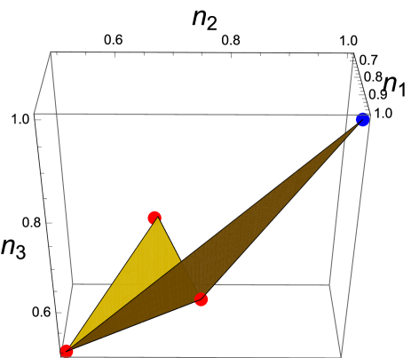
Figure 1: The hyperplanes $2=n_{1}+n_{2}+n_{4}$ and $2=n_{1}+n_{2}+n_{3}$, subject to the conditions $1\geq n_{1}\geq n_{2}\geq n_{3}\geq 0.5$ and $2\geq n_{1}+n_{2}+n_{4}$. The blue dot is the Hartree-Fock point $\bigl{(}1,1,1\bigr{)}$. The red ones are $\bigl{(}1,\tfrac{1}{2},\tfrac{1}{2}\bigr{)}$, $\bigl{(}\tfrac{3}{4},\tfrac{3}{4},\tfrac{1}{2}\bigr{)}$ and $\bigl{(}\tfrac{2}{3},\tfrac{2}{3},\tfrac{2}{3}\bigr{)}$.

III.2 Correlations

In Fig. 1 we illustrate the discussion of the previous section, highlighting four special configurations, namely:

• The “Hartree-Fock” point $(n_{1},n_{2},n_{3})=\bigl{(}1,1,1\bigr{)}$, which corresponds to the single Slater determinant $|\varphi_{1}\varphi_{2}\varphi_{3}\rangle$. Note that it does not coincide in general with the Hartree-Fock state, since it is described in the natural-orbital basis set. However, we call it so because its spectrum is $\vec{n}_{\rm HF}=(1,1,1,0,0,0)$.

• The point $\mathcal{P}_{a}\equiv\bigl{(}\tfrac{2}{3},\tfrac{2}{3},\tfrac{2}{3}\bigr{)}$, which corresponds to the strongly (static) correlated state:

  $$\mbox{$|\Psi_{a}\rangle$}=\tfrac{1}{\sqrt{3}}(\mbox{$|\varphi_{1}\varphi_{2}\varphi_{4}\rangle$}+\mbox{$|\varphi_{1}\varphi_{3}\varphi_{5}\rangle$}+\mbox{$|\varphi_{2}\varphi_{3}\varphi_{6}\rangle$}).$$ (13)

• The point $\mathcal{P}_{b}\equiv\bigl{(}1,\tfrac{1}{2},\tfrac{1}{2}\bigr{)}$. These occupation numbers correspond to the state

  $$\mbox{$|\Psi_{b}\rangle$}=\tfrac{1}{\sqrt{2}}(\mbox{$|\varphi_{1}\varphi_{2}\varphi_{3}\rangle$}+\mbox{$|\varphi_{1}\varphi_{4}\varphi_{5}\rangle$}).$$ (14)

  In quantum information theory, this state is said to be biseparable because one of the particles is disentangled from the other ones Lévay and Vrana (2008).

• The point $\mathcal{P}_{c}\equiv\bigl{(}\tfrac{3}{4},\tfrac{3}{4},\tfrac{1}{2}\bigr{)}$, which correspond to the (static) correlated state:

  $$\mbox{$|\Psi_{c}\rangle$}=\tfrac{1}{\sqrt{2}}\mbox{$|\varphi_{1}\varphi_{2}\varphi_{3}\rangle$}+\tfrac{1}{2}(\mbox{$|\varphi_{1}\varphi_{4}\varphi_{5}\rangle$}+\mbox{$|\varphi_{2}\varphi_{4}\varphi_{6}\rangle$}).$$ (15)

  Points $\mathcal{P}_{b}$ and $\mathcal{P}_{c}$ lie in the intersection of $\mathcal{A}_{1}$ and $\mathcal{A}_{2}$, namely, the degeneracy line $n_{3}=n_{4}=\tfrac{1}{2}$. Since $n_{3}$ and $n_{4}$ are identical, the choice of the highest occupied natural orbital $|\varphi_{3}\rangle$ and the lowest unoccupied natural orbital $|\varphi_{4}\rangle$ is not unique anymore and the indices $3$ and $4$ can be swapped in (14) and (15) without changing the spectra.

These four points are important because they belong to two different correlation regimes. On the one hand, the states $|\Psi_{a}\rangle$ and $|\Psi_{b}\rangle$ exhibit static correlation, as they are equiponderant superpositions of Slater determinants. On the other, the state $|\Psi_{c}\rangle$ is the superposition of two states ($|\varphi_{1}\varphi_{4}\varphi_{5}\rangle$ and $|\varphi_{2}\varphi_{4}\varphi_{6}\rangle$) and the nearly degenerate $|\varphi_{1}\varphi_{4}\varphi_{5}\rangle$ and its correlation is also static. This is reminiscent of the zero-order description of the beryllium ground state, for which the $2s$ and $2p$ orbitals are nearly degenerate and the state is a equiponderant superposition of three Slater determinants plus a highly weighted reference state Tew, Klopper, and Helgaker (2007).

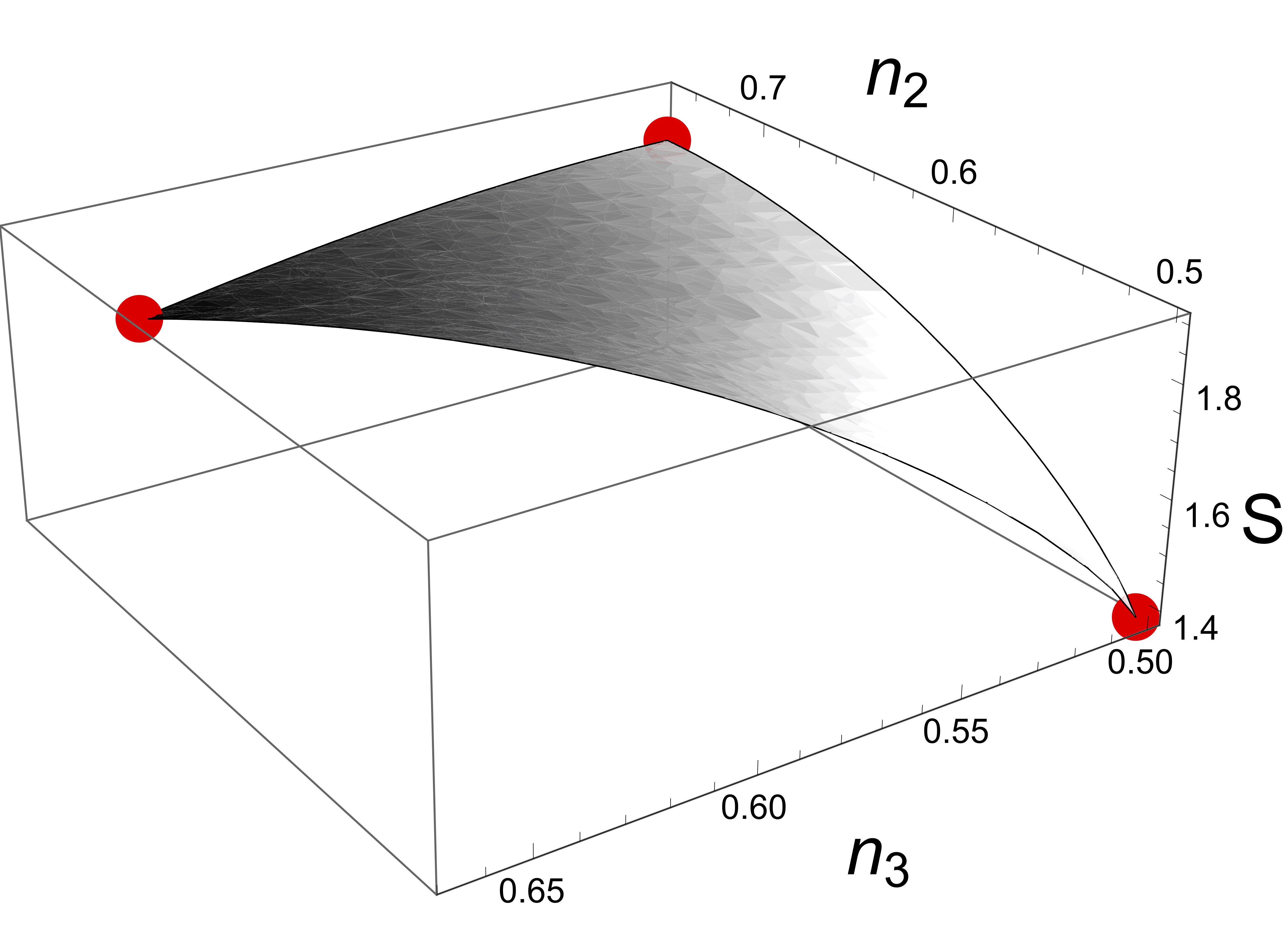
Figure 2: Entanglement entropy of the hyperplanes $\mathcal{A}_{1}$ and $\mathcal{A}_{2}$.

In Fig. 2 the entanglement entropy $S=-\sum_{i}n_{i}\ln n_{i}$ is plotted as a function of $n_{2}$ and $n_{3}$ for the hyperplanes $\mathcal{A}_{1}$ and $\mathcal{A}_{2}$. The entanglement entropy of the state $|\varphi_{1}\varphi_{2}\varphi_{3}\rangle$ is zero since it is uncorrelated. The entropies of the states $|\Psi_{b}\rangle$ and $|\Psi_{c}\rangle$ are 1.3862 and 1.8178, respectively. As one might expect, the configurations present in $\mathcal{A}_{2}$ all are strongly correlated. For the highest correlated state $|\Psi_{a}\rangle$, $S=1.9095$. The particular structure of the states $|\Psi_{a}\rangle$, $|\Psi_{b}\rangle$ and $|\Psi_{c}\rangle$ prompts us to say that the correlation effects of the states lying in the hyperplane $\mathcal{A}_{2}$ are all due to static effects, while the states in $\mathcal{A}_{1}$ are due to both static and dynamic effects.

According to the particle-hole symmetry, when applied to a three-electron system, the nonzero eigenvalues and their multiplicities are the same for the one- and the two-body reduced matrices. Thus, the results in this section based on one-particle information alone are also valid at the level of the 2-particle picture.

III.3 Borland-Dennis for three active electrons

In the configuration interaction picture, the full wavefunction is to be expressed in a given one-electron basis as a linear combination of all possible Slater determinants, save symmetries. In the basis of natural orbitals, it reads:

$$\mbox{$|\Psi\rangle$}=\sum_{1\leq i_{1}<\cdots<i_{N}\leq d}c_{i_{1}\ldots i_{N}}\mbox{$|\varphi_{i_{1}}\ldots\varphi_{i_{N}}\rangle$}$$ (16)

in a similar fashion to the Hartree-Fock ansatz (4). It is well known that the expansion (16) contains a very large number of configurations that are superfluous or negligible for computing molecular electronic properties. In practice, the configurations considered effective are sparse if an arbitrary threshold for the value of the amplitudes in (16) is enforced Mentel et al. (2014). As such, one often introduces the notion of active space to select the most relevant configurations at the level of the one-particle picture. A complete active space classifies the one-particle Hilbert space in core (fully occupied), active (partially occupied) and virtual (empty) spin-orbitals. The core spin-orbitals are pinned (completely populated) and are not treated as correlated. Adding active-space constraints improves the estimate of the ground-state energy in the framework of reduced-density-matrix theory Shenvi and Izmaylov (2010).

The generalized Pauli principle can shed some light on this important concept Tennie, Vedral, and Schilling (2017); Schilling, Benavides-Riveros, and Vrana (2017). In fact, for the case of $r$ core (and consequently $d-r$ active orbitals) the Hilbert space $\mathcal{H}_{N,d}$ is isomorphic to the wedge product $\mathcal{H}^{\rm core}_{r,r}\wedge\mathcal{H}^{\rm active}_{N-r,d-r}$. Hence, a wave function $\mbox{$|\Psi\rangle$}\in\mathcal{H}_{N,d}$ can be written in the following way:

$$\mbox{$|\Psi\rangle$}=\mbox{$|\varphi_{1}\dots\varphi_{r}\rangle$}\wedge\mbox{$|\Psi^{\rm active}\rangle$},$$ (17)

where $\mbox{$|\Psi^{\rm active}\rangle$}\in\mathcal{H}^{\rm active}_{N-r,d-r}$. The first $r$ natural occupation numbers are saturated to $1$. The remaining $d-r$ occupation numbers $(n_{r+1},\dots,n_{d})$ satisfy a set of generalized Pauli constraints and lie therefore inside the polytope $\mathcal{P}_{N-r,d-r}$. The space $\mathcal{H}^{\rm active}_{N-r,d-r}$ is called here the “active Hilbert space”. For instance, for the “Hartree-Fock” space $\mathcal{H}_{N,N}$, the corresponding zero dimensional active Hilbert space is $\mathcal{H}^{\rm active}_{0,0}$.

It is possible to characterize a hierarchy of active spaces by the effective dimension of $\mathcal{H}^{\rm active}_{N-r,d-r}$ and the number of Slater determinants appearing in the configuration interaction expansion of $|\Psi^{\rm active}\rangle$ Tennie, Vedral, and Schilling (2017); Schilling, Benavides-Riveros, and Vrana (2017). For the “active” Borland-Dennis setting $\mathcal{H}^{\rm active}_{3,6}$ we can apply the same considerations discussed in the last subsections: if the corresponding constraint (6) is saturated, the wave function fulfills $(\hat{n}_{r+1}+\hat{n}_{r+2}+\hat{n}_{r+4})\mbox{$|\Psi\rangle$}=2\mbox{$|\Psi\rangle$}$, and the set of possible Slater determinants reduces to just three, taking thus the form:

$$|\Psi^{\rm active}\rangle =\sqrt{n_{r+3}}\mbox{$|\varphi_{r+1}\varphi_{r+2}\varphi_{r+3}\rangle$}+\sqrt{n_{r+5}}\mbox{$|\varphi_{r+1}\varphi_{r+4}\varphi_{r+5}\rangle$}$$

$$+\sqrt{n_{r+6}}\mbox{$|\varphi_{r+2}\varphi_{r+4}\varphi_{r+6}\rangle$},$$ (18)

provided that $n_{r+3}\geq\tfrac{1}{2}$ and $n_{r+3}\geq n_{r+5}+n_{r+6}$.

IV Correlations and correlation measures

Even if the peculiar role played by electronic correlations in quantum mechanics were noticed from the onset, the problem of how to measure quantum correlations is still subject to an intense research Horodecki et al. (2009); Szalay (2015). The degree of entanglement $\mathcal{D}(\Psi)$ of an arbitrary vector $|\Psi\rangle$ can be expressed by its projection onto the nearest normalized unentangled (or uncorrelated) pure state Shimony (1995); Myers and Wu (2010):

$$\mathcal{D}(\Psi)=1-\max_{\Phi}|\langle\Psi\mbox{$|\Phi\rangle$}|^{2},$$ (19)

where the maximum is over all unentangled states, normalized so that $\langle\Phi\mbox{$|\Phi\rangle$}=1$. Although this measures sound conventional, it has the merit of being zero whenever $|\Psi\rangle$ is uncorrelated.

This measure (and the minimum $\min_{\tilde{\Phi}\in\mathcal{F}}||\Psi-\tilde{\Phi}||^{2}$, where $\mathcal{F}$ denotes the set of unnormalized unentangled (or uncorrelated) pure statesShimony (1995)) is also important in the realm of quantum chemistry. In the Appendix we state and prove that the set of pure quantum systems with predetermined energy is connected: given a Hamiltonian $\hat{H}$ there are two wavefunctions $|\psi_{1}\rangle$ and $|\psi_{2}\rangle$ with energies $E_{1}$ and $E_{2}$ whose distance $||\psi_{1}-\psi_{2}||^{2}$ is bounded by a function of $|E_{1}-E_{2}|$ (see Theorem 2 in the Appendix). Recently, we have shown that when $|\Psi\rangle$ is the ground state of a given Hamiltonian the measure (19) is closely related to the concept of correlation energy as understood in quantum chemistry Benavides-Riveros et al. (2017). A key ingredient in such connection turns out to be the energy gap within the symmetry-adapted Hilbert subspace.

IV.1 Dynamic correlation

The $N$-particle description of a quantum system and its reduced one-fermion picture can be related in meaningful ways. In effect, $\mathcal{D}(\Psi)$ can be bounded from above and from below by the $l^{1}$-distance of the natural occupation numbers. In fact, the distance between a wave function $|\Psi\rangle$ and any Slater determinant $|\varphi_{i_{1}}\dots\varphi_{i_{N}}\rangle$ satisfies Schilling, Gross, and Christandl (2013):

$$\frac{\delta_{\bm{i}}(\vec{n})}{2\min(N,d-N)}\leq 1-|\mbox{$\langle\varphi_{i_{1}}\dots\varphi_{i_{N}}|$}\Psi\rangle|^{2}\leq\frac{\delta_{\bm{i}}(\vec{n})}{2},$$ (20)

where $d$ is the dimension of the underlying one-particle Hilbert space, as defined in Sec. II, and $\delta_{\bm{i}}(\vec{n})\equiv\sum_{i\in\bm{i}}(1-n_{i})+\sum_{i\notin\bm{i}}n_{i}$ is the $l^{1}$-distance between $\vec{n}$ (the natural occupation numbers of $|\Psi\rangle$) and the natural occupation numbers of the Slater determinant in display (here $\bm{i}\equiv\{i_{1},\dots,i_{N}\}$). This result is also valid for Hartree-Fock or Brueckner orbitals Benavides-Riveros et al. (2017); Zhang and Kollar (2014). In particular, the $l^{1}$-distance to the Hartree-Fock point is given by:

$$\delta_{\rm HF}(\vec{n})=\sum_{i\leq N}(1-n_{i})+\sum_{i>N}n_{i}.$$ (21)

In Fig. 3 we plot $\delta_{\rm HF}(\vec{n})/2$ for the points in the hyperplane $\mathcal{A}_{1}$. As expected, $\delta_{\rm HF}(\vec{n}_{\rm HF})=0$. More interesting, the correlation increases monotonically with $n_{3}$. All the points on the degeneracy line $n_{3}=n_{4}$ are at the same $l^{1}$-distance from the Hartree-Fock point. In effect, $\delta_{\rm HF}(\vec{n}_{\rm s}(\eta))/2=1$, where

$$\vec{n}_{\rm s}(\eta)\equiv(\tfrac{3}{4}+\eta,\tfrac{3}{4}-\eta,\tfrac{1}{2},\tfrac{1}{2},\tfrac{1}{4}+\eta,\tfrac{1}{4}-\eta),$$ (22)

with $0\leq\eta\leq\tfrac{1}{4}$, is the set of points lying on the intersection line $n_{3}=n_{4}=\tfrac{1}{2}$. Moreover, $\delta_{\rm HF}(\mathcal{A}_{2})/2=1$, for all the points lying on the hyperplane $\mathcal{A}_{2}$.

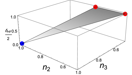
Figure 3: $l^{1}$-distance of the hyperplane $\mathcal{A}_{1}$ with respect to the Hartree-Fock point $\vec{n}_{\rm HF}$.

IV.2 Static correlation

Roughly speaking, the idea of static correlation is associated with the presence of a wave function built up from an equiponderant superposition of more than one Slater determinant, namely,

$$\frac{1}{\sqrt{m}}(\mbox{$|\Phi_{1}\rangle$}+\cdots+\mbox{$|\Phi_{m}\rangle$}),$$ (23)

For the Borland-Dennis setting $\mathcal{H}_{3,6}$, the hyperplane $\mathcal{A}_{2}$ contains states with three configurations being almost equiponderant. After this long discussion, it is natural to define all the points lying on the hyperplane $\mathcal{A}_{2}$ as statically correlated. The hyperplane $\mathcal{A}_{1}$ contains the uncorrelated Hartree-Fock state and the correlation of the rest of the states present is due to static as well as dynamic effects.

The “static” states $|\Psi_{\rm s}(\eta)\rangle$ that lead to the occupancies $\vec{n}_{\rm s}(\eta)$ as defined in Eq. (22) read:

$$\mbox{$|\Psi_{\rm s}(\eta)\rangle$}\equiv\tfrac{1}{\sqrt{2}}\mbox{$|\varphi_{1}\varphi_{2}\varphi_{3}\rangle$}+\sqrt{\tfrac{1}{4}+\eta}\mbox{$|\varphi_{1}\varphi_{4}\varphi_{5}\rangle$}+\sqrt{\tfrac{1}{4}-\eta}\mbox{$|\varphi_{2}\varphi_{4}\varphi_{6}\rangle$},$$ (24)

where $0\leq\eta\leq\tfrac{1}{4}$. As stated before, since $n_{3}$ and $n_{4}$ are identical, the choice of the highest occupied natural orbital and the lowest unoccupied natural orbital is not unique and the indices 3 and 4 can be swapped without changing the spectra. However, by doing so the resulting state is orthogonal to $|\varphi_{1}\varphi_{2}\varphi_{3}\rangle$.

The $L^{2}$-distance (Eq. (19)) between the Borland-Dennis state (11) and $|\Psi_{\rm s}(\eta)\rangle$ is given by $\mathcal{J}_{\rm s}(\eta)\equiv 1-|\langle\Psi_{\rm BD}\mbox{$|\Psi_{\rm s}(\eta)\rangle$}|^{2}$. The minimum of this distance depends only on the value of the natural occupation number corresponding to the highest occupied natural orbital. To see this notice that the minimum of $\mathcal{J}_{\rm s}(\eta)$ is attained when $d\mathcal{J}_{\rm s}(\eta)/d\eta=0$, which happens at $\eta^{*}=\frac{n_{5}-n_{6}}{4(1-n_{3})}.$ The distance is therefore

$$\mathcal{J}_{\rm s}(\eta^{*}) =1-\bigg{(}\frac{\sqrt{n_{3}}}{\sqrt{2}}+\frac{1-n_{2}}{\sqrt{2(1-n_{3})}}+\frac{n_{2}-n_{3}}{\sqrt{2(1-n_{3})}}\bigg{)}^{2}$$

$$=1-\tfrac{1}{2}(\sqrt{n_{3}}+\sqrt{1-n_{3}})^{2}=\tfrac{1}{2}-\sqrt{n_{3}(1-n_{3})},$$ (25)

which is zero when the correlation of the Borland-Dennis state is completely static and is $\tfrac{1}{2}$ when the state is the uncorrelated Hartree-Fock state.

We can also investigate the $l^{1}$-distance between any state $\vec{n}\in\mathcal{A}_{1}$ and the state $\vec{n}_{\rm s}(\eta)$ (22), namely:

$$\delta_{\rm s}(\vec{n})=\min_{\eta}dist_{1}(\vec{n},\vec{n}_{s}(\eta)).$$ (26)

Notice that the $l^{1}$-distance reads

$$dist_{1}(\vec{n},\vec{n}_{s}(\eta))=2(|n_{1}-(\tfrac{3}{4}+\eta)|+|n_{2}-(\tfrac{3}{4}-\eta)|+|n_{3}-\tfrac{1}{2}|).$$

So, to minimize $dist_{1}(\vec{n},\vec{n}_{s}(\eta))$ is the same as minimizing $|n_{1}-\tfrac{3}{4}-\eta|+|n_{2}-\tfrac{3}{4}+\eta|$. Since the $l^{1}$-sphere with radius $z$ centered at $\vec{n}$ is the convex hull of the vertices $((n_{1}\pm z,n_{2},n_{3}),(n_{1},n_{2}\pm z,n_{3}),(n_{1},n_{2},n_{3}\pm z))$, the minimum of the distance is:

$$\delta_{\rm s}(\vec{n}) =2(|n_{1}-(-n_{2}+\tfrac{3}{2})|+|n_{3}-\tfrac{1}{2}|)=4(n_{3}-\tfrac{1}{2}),$$ (27)

which depends on $n_{3}$ alone. Notice that for the Hartree-Fock point $\delta_{\rm s}(\vec{n}_{\rm HF})/2=1$ and remember that by our definition $\delta_{\rm s}(\vec{n})=0$ if $\vec{n}\in\mathcal{A}_{2}$. Remarkably, $\eta^{*}$, the minimizer of $\mathcal{J}_{\rm s}(\eta)$, is also a minimizer of $dist_{1}(\vec{n},\vec{n}_{s}(\eta))$. This latter statement can be proved by noting that the first occupation number of $\vec{n}_{s}(\eta_{*})$ satisfies

$$n_{1}(\eta^{*})=\frac{3}{4}+\frac{n_{1}-n_{2}}{4(1-n_{3})}=\frac{2-4n_{3}+2n_{1}}{4(1-n_{3})}\leq\frac{n_{1}}{2(1-n_{3})}\leq n_{1},$$

since $n_{3}\geq\tfrac{1}{2}$. Equivalently, $n_{2}(\eta^{*})\leq n_{2}$. Therefore:

$$dist_{1}(\vec{n},\vec{n}_{s}(\eta^{*})) =2[(n_{1}-\tfrac{3}{4}-\eta_{*})+(n_{2}-\tfrac{3}{4}+\eta^{*})+(n_{3}-\tfrac{1}{2})]$$

$$=2[(n_{1}+n_{2}-\tfrac{3}{2})+(n_{3}-\tfrac{1}{2})]=4(n_{3}-\tfrac{1}{2}),$$

which is the minimum (27).

IV.3 Correlation measures

The comparison of the distances (21) and (26) allows us to distinguish between dynamic and static correlations. The distance to the Hartree-Fock point $\delta_{\rm HF}(\vec{n})$ can be viewed as a measure of the dynamic part of the electronic correlation, for it quantifies how much a wave function differs from the uncorrelated Hartree-Fock state. The static distance $\delta_{\rm s}(\vec{n})$ can be viewed as a measure of the static part of the correlation, as it quantifies how much a wave function differs from the set of static states. One expects for helium $\delta_{\rm HF}(\vec{n}_{\rm He})\approx 0$ while for H₂ at infinite separation $\delta_{\rm s}(\vec{n}_{{\rm H}_{2,\infty}})=0$. For convenience we renormalize these two $l^{1}$-distances by means of

$$P_{\rm sta}(\vec{n})=\frac{\delta_{\rm HF}(\vec{n})}{\delta_{\rm HF}(\vec{n})+\delta_{\rm s}(\vec{n})}\quad{\rm and}\quad P_{\rm dyn}(\vec{n})=\frac{\delta_{\rm s}(\vec{n})}{\delta_{\rm HF}(\vec{n})+\delta_{\rm s}(\vec{n})}.$$ (28)

Since the measures $P_{\rm dyn}(\vec{n})$ and $P_{\rm sta}(\vec{n})$ are normalized (while $\delta_{\rm HF}(\vec{n})$ and $\delta_{\rm s}(\vec{n})$ are not), they are much more useful to compare different systems. In this way, when the correlation is due to static effects $P_{\rm sta}(\vec{n})=1$ and $P_{\rm dyn}(\vec{n})=0$, while the contrary occurs for a completely dynamic state. For instance, one expects for He $P_{\rm sta}(\vec{n}_{\rm He})\approx 0$ while for H₂ at infinite separation $P_{\rm dyn}(\vec{n}_{{\rm H}_{2,\infty}})=0$. These quantities have the merit of being zero or one when the correlation is completely dynamic or completely static and hence they separate the correlation in two contributions.

It is worth saying that our considerations do not only apply for the Borland-Dennis setting but also for larger ones. Recall that for the settings $\mathcal{H}_{N,d}$ and $\mathcal{H}_{N,d^{\prime}}$, such that $d<d^{\prime}\in{\mathbb{N}}$, the corresponding polytopes satisfy: $\mathcal{P}_{N,d}={\mathcal{P}_{N,d^{\prime}}}|_{n_{d+1}=\cdots=n_{d^{\prime}}=0}$. It means that, intersected with the hyperplane given by $n_{d+1}=\cdots=n_{d^{\prime}}=0$, the polytope $\mathcal{P}_{N,d^{\prime}}$ coincides with $\mathcal{P}_{N,d}$ Schilling, Gross, and Christandl (2013). Therefore, we have completely characterized the static states up to six dimensional one-particle Hilbert spaces. By choosing $n_{1}=1$, we freeze one electron, we are effectively dealing with a two active-electron system and our measures can also be used for characterizing the correlation of two-electron systems. Note that for this latter case the natural occupation numbers are evenly degenerated, a very well known representability condition for systems with a even number of electrons and time-reversal symmetry Smith (1966).

V Correlation in molecular systems

To illustrate these concepts we plot in Fig. 4 our measures of static and dynamic correlation for the ground states of the diatomic molecules H₂ and Li₂ as a function of the interatomic distance. In the same plot we can also see the von-Neumann entropy and the value of the highest occupancy of the highest occupied natural spin-orbital. These numbers were obtained from CAS-SCF calculation using the code Gamess Schmidt et al. (1993) and cc-pVTZ basis sets with all electrons active and as large as possible active space of orbitals.

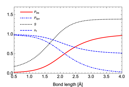
(a) H₂.

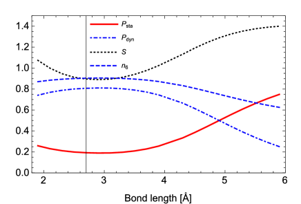
(b) Li₂.

Figure 4: Correlation curves for H₂ and Li₂. $P_{\rm sta}$ and $P_{\rm dyn}$ as well as the occupancy of the highest occupied natural spin-orbital and the von Neumann entropy $S$ are plotted as functions of the interatomic distance (in Å). The equilibrium bonding length is 0.74 Å for H₂ and 2.67 Å for Li₂.

The molecule H₂, and in particular its dissociation limit, is the quintessential example of static correlation Coulson and Fischer (1949). It is well known that the restricted Hartree-Fock approach describes very well the equilibrium chemical bond, but fails dramatically as the molecule is stretched. Around the equilibrium separation, $P_{\rm sta}$ is close to zero and $P_{\rm dyn}$ reaches its maximum. There is a change of regime around $1.5$ Å because the static correlation begins to grow rapidly. Beyond this point, restricted Hartree-Fock theory is unable to predict a bound system anymore. At the dissociation limit, the correlation is due to static effects only, as expected. Both measures allow us to observe the smooth increasing of static effects when the molecule is elongated. A different situation can be observed for the diatomic Li₂. For lengths smaller than the bond length the static correlation decreases as the distance increases. The energy, the static correlation and the von-Neumann entropy reach their minimum around $2.9$ Å, very close to the equilibrium bonding length, while the dynamic correlation as well as the occupancy of the highest occupied natural spin-orbital acquired their maximum. Beyond that value, the static correlation grows and the dynamic correlation decreases slowly. This behaviour changes around $4$ Å, where the static correlation speeds up.

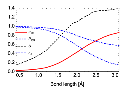
(a) H₃.

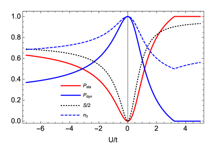
(b) Three-fermion three-site Hubbard model.

Figure 5: Correlation curves for H₃ and the three-fermion three-site Hubbard model. $P_{\rm sta}$ and $P_{\rm dyn}$ as well as the occupancy of the highest occupied natural spin-orbital and the von Neumann entropy $S$ are plotted as functions of the interatomic distance (in Å) or the coupling strength.

In Fig. 5 we plot the correlation measures for three-electron systems: the ground state of the equilateral H₃ and the three-site three-fermion Hubbard model, which is very well known for it is analytically solvable Benavides-Riveros et al. (2017); Schilling (2015b). The Hamiltonian (in second quantization) of the one-dimensional $r$-site Hubbard model reads:

$$\hat{H}=-\frac{t}{2}\sum_{i,\sigma}(c^{\dagger}_{i\sigma}c_{(i+1)\sigma}+h.c.)+2U\sum_{i}\hat{n}_{i\uparrow}\hat{n}_{i\downarrow},$$ (29)

$i\in\{1,2,\dots,r\}$, where $c^{\dagger}_{i\sigma}$ and $c_{i\sigma}$ are the fermionic creation and annihilation operators for a particle on the site $i$ with spin $\sigma\in\{\uparrow,\downarrow\}$ and $\hat{n}_{i\sigma}=c^{\dagger}_{i\sigma}c_{i\sigma}$. The first term in Eq. (29) describes the hopping between two neighboring sites while the second represents the on-site interaction. Periodic boundary conditions for the case $r=3$ are also assumed. Achieved experimentally very recently with full control over the quantum state Murmann et al. (2015), this model may be considered as a simplified tight-binding description of the H_r molecule. For the case of H₃ the correlation measures are plotted as a function of the interatomic distance (in Å) and for the Hubbard model as a function of the coupling $U/t$. In both cases, as the molecule is elongated or the interaction in the Hubbard model is enhanced, the energy gap (the energy difference between the first-excited and the ground states) shortens and the electronic correlation increases, leading to the appearance of static effects Benavides-Riveros et al. (2017). While H₃ exhibits a behaviour essentially similar to H₂, the Hubbard model shows off two different regimes of correlation. For positive values of the relative coupling, the static correlation plays a prominent role. In particular, beyond $U/t=3.2147$, the system lies in the hyperplane $\mathcal{A}_{2}$ of the Borland-Dennis setting (10) and the correlation is completely static. For this strongly correlated regime, the ground state can be written as a equiponderant superposition of three Slater determinants. For negative values of the coupling there is always a fraction of the correlation due to dynamic effects. In that limit the ground state is written as a superposition of two Slater determinants with different amplitudes.

It is known that static and dynamic electronic correlations play a prominent role in the orthogonally twisted ethylene Zen et al. (2014). In fact, the energy gap between the ground and the first excited state shortens when the torsion angle around the C$=$C double bond is increased. While the ground state of the planar ethylene is very well described by a single Slater determinant, at ninety degrees at least two Slater determinants are needed, resembling the dihydrogen in the dissociation limit. In Fig. 6 we plot the correlation energy and the energy gap of ethylene as a function of the torsion angle, using CAS-SCF(12,12) method and a cc-pVDZ basis set. In Fig. 7 we plot the correlation measures for ethylene along the torsional path. For the planar geometry the correlation is almost completely dynamic and the situation remains in this way until the torsional degree reaches 60^o. From this angle on the static correlation shows up. At 80^o the static and dynamic correlation are equally important in the total electron correlation of ethylene. When orthogonally twisted, the correlation of ethylene is 90% due to static effects and there is still an important part due to dynamic correlation. Remarkably, the rise of static correlation around 60^o coincides with the increase of correlation energy. From this perspective, the gain of total correlation is mainly due to static effects.

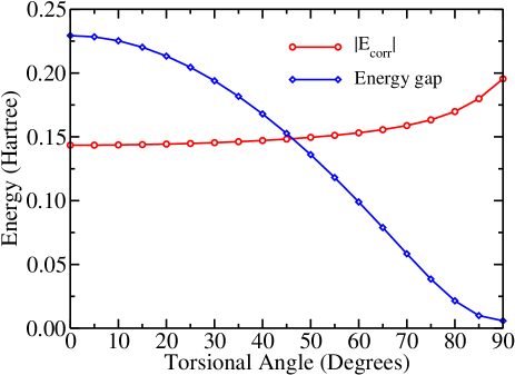
Figure 6: Correlation energy and energy gap for the twisted ethylene C₂H₄ as a function of the torsion angle around the C=C double bond.

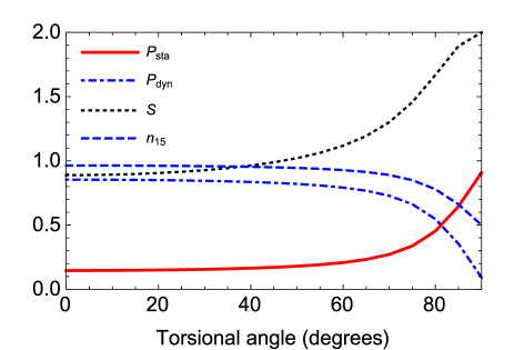
Figure 7: Correlation curves for ethylene. $P_{\rm sta}$ and $P_{\rm dyn}$ as well as the occupancy of the highest occupied natural spin-orbital and the von Neumann entropy $S$ are plotted as functions of the torsion angle around the C=C double bond.

VI Summary and conclusion

Thanks to the generalization of the Pauli exclusion principle, it is possible to relate equiponderant superpositions of Slater determinants to certain sets of fermionic occupation numbers lying inside the Paulitope. In this paper, we have proposed a general criterion to distinguish the static and dynamic parts of the electronic correlation in fermionic systems, by tackling only one-particle information. By doing so, we provided two kinds of $l^{1}$-distances: (a) to the Hartree-Fock point, which can be viewed as a measure of the dynamic part of the electronic correlation, and (b) to the static states, which can be viewed as a measure of the static part of the correlation. We gave some examples of physical systems and showed that these correlation measures correlate well with our intuition of static and dynamic correlation.

Though we focused our attention on two and three “active”-fermion systems, the results can in principle be generalized to larger settings. So far, the complete set of generalized Pauli constraints is only known for small systems with three, four and five particles. There is, however, an algorithm which provide in principle the representability conditions for larger settings Klyachko (2006).

In this paper we have highlighted the paramount importance of the occupancy of the highest occupied natural spin-orbital in the understanding of the static correlation. The quantities we proposed in this paper can allow us to construct reliable ways to separate dynamic and static correlations and, more important, to better understand the qualitative nature of the correlation present in real physical and chemical electronic systems. They can also be a tool for analysing the failures of quantum many body theories (like density functional theory) Chai (2012). Recent progress in fermionic mode entanglement can also shed more light in these directions Boguslawski et al. (2013); Friis (2016).

References

- Tew, Klopper, and Helgaker (2007) D. P. Tew, W. Klopper, and T. Helgaker, J. Comput. Chem. 28, 1307 (2007).
- Wigner (1934) E. Wigner, Phys. Rev. 46, 1002 (1934).
- Löwdin (1955) P.-O. Löwdin, Phys. Rev. 97, 1509 (1955).
- Casula and Sorella (2003) M. Casula and S. Sorella, J. Chem. Phys. 119, 6500 (2003).
- Casula, Attaccalite, and Sorella (2004) M. Casula, C. Attaccalite, and S. Sorella, J. Chem. Phys. 121, 7110 (2004).
- Zen et al. (2014) A. Zen, E. Coccia, Y. Luo, S. Sorella, and L. Guidoni, J. Chem. Theory Comput. 10, 1048 (2014).
- Neuscamman (2013) E. Neuscamman, J. Chem. Phys. 139, 194105 (2013).
- Schliemann et al. (2001) J. Schliemann, J. I. Cirac, M. Kuś, M. Lewenstein, and D. Loss, Phys. Rev. A 64, 022303 (2001).
- Plastino, Manzano, and Dehesa (2009) A. R. Plastino, D. Manzano, and J. S. Dehesa, EPL 86, 20005 (2009).
- Sárosi and Lévay (2014) G. Sárosi and P. Lévay, Phys. Rev. A 89, 042310 (2014).
- Juhász and Mazziotti (2006) T. Juhász and D. A. Mazziotti, J. Chem. Phys. 125, 174105 (2006).
- Gottlieb and Mauser (2005) A. D. Gottlieb and N. J. Mauser, Phys. Rev. Lett. 95, 123003 (2005).
- Benavides-Riveros et al. (2017) C. L. Benavides-Riveros, N. N. Lathiotakis, C. Schilling, and M. A. L. Marques, Phys. Rev. A 95, 032507 (2017).
- Becke (2013) A. D. Becke, J. Chem. Phys. 138, 074109 (2013).
- Ziesche et al. (1997) P. Ziesche, O. Gunnarsson, W. John, and H. Beck, Phys. Rev. B 55, 10270 (1997).
- Cohen, Mori-Sánchez, and Yang (2008a) A. J. Cohen, P. Mori-Sánchez, and W. Yang, Science 321, 792 (2008a).
- Cohen, Mori-Sánchez, and Yang (2008b) A. J. Cohen, P. Mori-Sánchez, and W. Yang, J. Chem. Phys. 129, 121104 (2008b).
- Hollett and Gill (2011) J. W. Hollett and P. M. W. Gill, J. Chem. Phys. 134, 114111 (2011).
- Hollett, Hosseini, and Menzies (2016) J. W. Hollett, H. Hosseini, and C. Menzies, J. Chem. Phys. 145, 084106 (2016).
- Walter et al. (2013) M. Walter, B. Doran, D. Gross, and M. Christandl, Science 340, 1205 (2013).
- Sawicki, Walter, and Kuś (2013) A. Sawicki, M. Walter, and M. Kuś, J. Phys. A 46, 055304 (2013).
- Ramos-Cordoba, Salvador, and Matito (2016) E. Ramos-Cordoba, P. Salvador, and E. Matito, Phys. Chem. Chem. Phys. 18, 24015 (2016).
- Klyachko (2006) A. Klyachko, J. Phys. 36, 72 (2006).
- Theophilou et al. (2015) I. Theophilou, N. Lathiotakis, M. Marques, and N. Helbig, J. Chem. Phys. 142, 154108 (2015).
- Mazziotti (2016) D. A. Mazziotti, Phys. Rev. A 94, 032516 (2016).
- DePrince (2016) A. E. DePrince, J. Chem. Phys. 145, 164109 (2016).
- Müller (1999) C. W. Müller, J. Phys. A 32, 4139 (1999).
- Coleman (1963) A. J. Coleman, Rev. Mod. Phys. 35, 668 (1963).
- Altunbulak and Klyachko (2008) M. Altunbulak and A. Klyachko, Commun. Math. Phys. 282, 287 (2008).
- Schilling, Gross, and Christandl (2013) C. Schilling, D. Gross, and M. Christandl, Phys. Rev. Lett. 110, 040404 (2013).
- Schilling (2014a) C. Schilling, in Mathematical Results in Quantum Mechanics, edited by P. Exner, W. König, and H. Neidhardt (World Scientific, 2014) Chap. 10, pp. 165–176.
- Note (1) Norbert Mauser coined the term “Paulitope” during the Workshop Generalized Pauli Constraints and Fermion Correlation, celebrated at the Wolfgang Pauli Institute in Vienna in August 2016.
- Schilling (2015a) C. Schilling, Phys. Rev. A 91, 022105 (2015a).
- Benavides-Riveros, Gracia-Bondia, and Springborg (2013) C. L. Benavides-Riveros, J. M. Gracia-Bondia, and M. Springborg, Phys. Rev. A 88, 022508 (2013).
- Chakraborty and Mazziotti (2014) R. Chakraborty and D. Mazziotti, Phys. Rev. A 89, 042505 (2014).
- Benavides-Riveros, Gracia-Bondía, and Springborg (2014) C. L. Benavides-Riveros, J. M. Gracia-Bondía, and M. Springborg, arXiv:1409.6435 (2014).
- Benavides-Riveros and Springborg (2015) C. L. Benavides-Riveros and M. Springborg, Phys. Rev. A 92, 012512 (2015).
- Chakraborty and Mazziotti (2015a) R. Chakraborty and D. A. Mazziotti, Int. J. Quantum Chem. 115, 1305 (2015a).
- Benavides-Riveros and Schilling (2016) C. L. Benavides-Riveros and C. Schilling, Z. Phys. Chem. 230, 703 (2016).
- Tennie, Vedral, and Schilling (2016) F. Tennie, V. Vedral, and C. Schilling, Phys. Rev. A 94, 012120 (2016).
- Tennie et al. (2016) F. Tennie, D. Ebler, V. Vedral, and C. Schilling, Phys. Rev. A 93, 042126 (2016).
- Tennie, Vedral, and Schilling (2017) F. Tennie, V. Vedral, and C. Schilling, Phys. Rev. A 95, 022336 (2017).
- Wang, Wang, and Lischka (2017) Y. Wang, J. Wang, and H. Lischka, Int. J. Quantum Chem. , e25376 (2017), e25376.
- Chakraborty and Mazziotti (2015b) R. Chakraborty and D. Mazziotti, Phys. Rev. A 91, 010101 (2015b).
- Schilling (2015b) C. Schilling, Phys. Rev. B 92, 155149 (2015b).
- Schilling (2014b) C. Schilling, Quantum marginal problem and its physical relevance, Ph.D. thesis, ETH-Zürich (2014b).
- Klyachko (2009) A. Klyachko, arXiv:0904.2009 (2009).
- Schilling, Benavides-Riveros, and Vrana (2017) C. Schilling, C. L. Benavides-Riveros, and P. Vrana, arXiv:1703.01612 (2017).
- Benavides-Riveros (2015) C. L. Benavides-Riveros, Disentangling the marginal problem in quantum chemistry, Ph.D. thesis, Universidad de Zaragoza (2015).
- Cleland, Booth, and Alavi (2010) D. Cleland, G. H. Booth, and A. Alavi, J. Chem. Phys. 132, 041103 (2010).
- Giner, Scemama, and Caffarel (2013) E. Giner, A. Scemama, and M. Caffarel, Can. J. Chem. 91, 879 (2013).
- Caffarel et al. (2016) M. Caffarel, T. Applencourt, E. Giner, and A. Scemama, “Recent progress in quantum monte carlo,” in Using CIPSI Nodes in Diffusion Monte Carlo (ACS, 2016) Chap. 2, pp. 15–46.
- Borland and Dennis (1972) R. Borland and K. Dennis, J. Phys. B 5, 7 (1972).
- Löwdin and Shull (1956) P.-O. Löwdin and H. Shull, Phys. Rev. 101, 1730 (1956).
- Kutzelnigg and Smith (1968) W. Kutzelnigg and V. H. Smith, Int. J. Quant. Chem. 2, 531 (1968).
- Bytautas et al. (2011) L. Bytautas, T. M. Henderson, C. A. Jiménez-Hoyos, J. K. Ellis, and G. E. Scuseria, J. Chem. Phys. 135, 044119 (2011).
- Bytautas, Scuseria, and Ruedenberg (2015) L. Bytautas, G. E. Scuseria, and K. Ruedenberg, J. Chem. Phys. 143, 094105 (2015).
- Lévay and Vrana (2008) P. Lévay and P. Vrana, Phys. Rev. A 78, 022329 (2008).
- Mentel et al. (2014) L. M. Mentel, R. van Meer, O. V. Gritsenko, and E. J. Baerends, J. Chem. Phys. 140, 214105 (2014).
- Shenvi and Izmaylov (2010) N. Shenvi and A. F. Izmaylov, Phys. Rev. Lett. 105, 213003 (2010).
- Horodecki et al. (2009) R. Horodecki, P. Horodecki, M. Horodecki, and K. Horodecki, Rev. Mod. Phys. 81, 865 (2009).
- Szalay (2015) S. Szalay, Phys. Rev. A 92, 042329 (2015).
- Shimony (1995) A. Shimony, Ann. N. Y. Acad. Sci. 755, 675 (1995).
- Myers and Wu (2010) J. M. Myers and T. T. Wu, Quantum Inf. Process. 9, 239 (2010).
- Zhang and Kollar (2014) J. M. Zhang and M. Kollar, Phys. Rev. A 89, 012504 (2014).
- Smith (1966) D. W. Smith, Phys. Rev. 147, 896 (1966).
- Schmidt et al. (1993) M. W. Schmidt, K. K. Baldridge, J. A. Boatz, S. T. Elbert, M. S. Gordon, J. H. Jensen, S. Koseki, N. Matsunaga, K. A. Nguyen, S. Su, T. L. Windus, M. Dupuis, and J. A. Montgomery, J. Comput. Chem. 14, 1347 (1993).
- Coulson and Fischer (1949) C. A. Coulson and I. Fischer, Philos. Mag. 40, 386 (1949).
- Murmann et al. (2015) S. Murmann, A. Bergschneider, V. M. Klinkhamer, G. Zürn, T. Lompe, and S. Jochim, Phys. Rev. Lett. 114, 080402 (2015).
- Chai (2012) J.-D. Chai, J. Chem. Phys. 136, 154104 (2012).
- Boguslawski et al. (2013) K. Boguslawski, P. Tecmer, G. Barcza, Ö. Legeza, and M. Reiher, J. Chem. Theory Comput. 9, 2959 (2013).
- Friis (2016) N. Friis, New J. Phys. 18, 033014 (2016).