Optimal Invariant Tests in an Instrumental Variables Regression With Heteroskedastic and Autocorrelated Errors

Abstract

This paper uses model symmetries in the instrumental variable (IV) regression to derive an invariant test for the causal structural parameter. Contrary to popular belief, we show that there exist model symmetries when equation errors are heteroskedastic and autocorrelated (HAC). Our theory is consistent with existing results for the homoskedastic model (Andrews, Moreira, and Stock (2006) and Chamberlain (2007)). We use these symmetries to propose the conditional integrated likelihood (CIL) test for the causality parameter in the over-identified model. Theoretical and numerical findings show that the CIL test performs well compared to other tests in terms of power and implementation. We recommend that practitioners use the Anderson-Rubin (AR) test in the just-identified model, and the CIL test in the over-identified model.

1 Introduction

In a regression model, the explanatory variable can be correlated with the error due to omitted variables. To solve this endogeneity problem, practitioners often look for instrumental variables (IVs). The instruments are valid if they are correlated with the endogenous variable but uncorrelated with the error. The instruments are said to be weak when their correlation with the endogenous explanatory variable is small. Under weak identification, standard estimators may be far from the true causality parameter, and commonly-used tests do not have correct size. Searching for valid IVs can, unfortunately, narrow down the choices to only weak instruments. Furthermore, techniques proposed to mitigate these problems can themselves have limitations. Cruz and Moreira (2005) show that the second-order bias for the two-stage least squares (2SLS) estimator is unreliable under weak identification. Lee, McCrary, Moreira, and Porter (2020) point out that the standard F¿10 rule for the t-ratio leads to important size distortions in practice, even in the just-identified model. They propose a novel tF procedure if practitioners wish to use the F statistic combined with the t-ratio.

With cross-sectional data, the errors in the IV model can be heteroskedastic. With time-series or panel data, errors can also be autocorrelated. For these more complex data generating processes (DGPs) for the errors, the asymptotic variance matrix of sample IV moments can be quite different from the one obtained from serially uncorrelated and homoskedastic errors. Consistent estimators for this variance are readily available: see Newey and West (1987) and Andrews (1991).

Andrews, Moreira, and Stock (2006) (abbreviated as AMS06 hereinafter) and Chamberlain (2007) show that symmetries exist in the IV model with homoskedastic errors when the variance is fixed. Up until the emergence of this project (Moreira and Ridder (2017)), it was widely accepted that there are no symmetries in the IV model with heteroskedastic and/or autocorrelated (HAC) errors. Indeed, at first sight, invariance does not seem applicable to the HAC-IV model. We argue that this view is incorrect. The HAC-IV has model symmetries if the HAC variance matrix is assumed to be known but not fixed, an important distinction from the method used by AMS06, Chamberlain (2007), and related papers, for homoskedastic and uncorrelated errors. We find the largest affine group which preserves the null hypothesis for the causality parameter. This allows us to find weights for the novel conditional integrated likelihood (CIL) test. This test is invariant and can be interpreted as the limit of a sequence of conditional weighted-average power (WAP) tests. Andrews and Mikusheva (2020) provide a general framework for decision rules in GMM. They do not propose a two-sided test, which is our main goal in this paper. Unlike the CIL test, other (limits of) conditional WAP tests can be severely biased, as the critique by Moreira and Moreira (2019) asserts.

In the just-identified model, the AR test is optimal within the classes of either unbiased or invariant tests, assuming the reduced-form variance mentioned above is known; see Moreira (2002, 2009), AMS06, and Moreira and Moreira (2019). In the over-identified model, the AR test is not efficient under the usual asymptotic theory. Several proposed tests are asymptotically optimal under standard asymptotics. Moreira and Ridder (2020) show that the Lagrange Multiplier/score (LM) and the conditional quasi-likelihood ratio (CQLR) tests can suffer severe power deficiencies when distinguishing the null from the alternative hypothesis should be easy. The weighted-average strongly unbiased (SU) tests are not invariant for arbitrary weight choices. Furthermore, implementing the SU tests requires linear programming. Although algorithms are readily available, it requires the calculation of a density ratio. If not dealt with properly, the computation can exceed the numerical accuracy of computer packages. This leaves, as the main contender, the true conditional likelihood ratio (CLR) test; see Andrews and Mikusheva (2016) and Moreira and Moreira (2019). The CLR test does not have a closed-form expression with HAC errors, and requires numerical optimization. We show some important limitations to the implementation of the CLR test. We prove here that we can compactify the parameter space for the optimization. This is important, and avoids some natural pitfalls if the parameter space is unbounded. However, we find that the number of initial points needed for the optimization algorithm depends on the errors’ DGPs and on the instrument strength. In practice, we document the need to include several initial points when errors are HAC. Worse yet, the optimization can be even more troublesome when computing the conditional quantiles. This happens because the model is misspecified for DGPs under the alternative hypothesis when we simulate these null conditional quantiles.

We then compare power between the AR, CLR, and CIL tests. For homoskedastic errors, the CLR test simplifies to the CQLR test, which has a closed-form expression. Andrews, Moreira, and Stock (2004) use these symmetries to choose weights for a conditional WAP test. Power gains beyond the CQLR are small, as the latter performs near a two-sided power envelope for invariant tests with homoskedastic errors. It is, however, reassuring that the CIL test performs on an equal footing with the CQLR test. For HAC errors, the IV model is much more complex than the simple homoskedastic model. Even reducing the data using invariance, several parameters can affect the performance of AR, LM, CQLR, CLR, CIL, and any other invariant tests. We choose the same designs as Moreira and Moreira (2019) and Moreira and Ridder (2020), to forestall any criticism that we may be selecting parameter combinations which favor the CIL test. To bypass the aforementioned numerical problems for the CLR test, we choose to implement an infeasible version of the CLR test, in case better optimization methods are found in the future. This implementation selects the unknown value of the structural parameter as one of the initial points in the likelihood optimization. Overall, the CIL test outperforms the AR and CLR tests, with significant power gains for several of these designs.

This paper is organized as follows. Section 2 introduces the IV model, and describes the family of similar tests robust to heteroskedastic-autocorrelated errors. Section 3 shows model symmetries when the asymptotic variance can change with data transformations. We present different representations of the CIL test. One of them is important to show that this test is invariant, as discussed later. The other expression is useful to derive confidence sets based on the CIL test. Section 4 shows that the CIL test can have very good power (the supplement provides further evidence in favor of the CIL test). The more technical details behind model invariance are left to the end of the paper. Section 5 shows that the theory of AMS06 is a special case of ours when the variance has a Kronecker product form. Section 6 derives the theory of conditional invariant tests. It shows that the AR, CLR, and Lagrange Multiplier/score (LM) tests are also invariant. Section 7 discusses the next steps in this research agenda and highlights the methodological importance of distinguishing between parameters being known and being fixed. The online appendix provides the proofs for our theory.

2 The IV Model and Statistics

2.1 The HAC-IV model

Consider the following structural equation for the $i$-th observation of the variable $y_{1}$:

$$y_{1i}=y_{2i}\beta+x_{i}^{\prime}\gamma_{1}+u_{i},\text{ for }i=1,2,\cdots,n,$$ (2.1)

where $y_{2i}$ is an endogenous random variable with corresponding coefficient $\beta\in\mathbb{R}$, $x_{i}=(x_{1i},x_{2i},\cdots,x_{pi})^{\prime}\in\mathbb{R}^{P}$ is a fixed vector of exogenous control variables with corresponding vector of coefficients $\gamma_{1}=(\gamma_{1}^{\ast},\gamma_{2}^{\ast},\cdots,\gamma_{p}^{\ast})^{\prime}\in\mathbb{R}^{p}$, and $u_{i}$ is an error term. We also consider the following reduced-form equation for the endogenous explanatory random variable:

$$y_{2i}=\tilde{z}_{i}^{\prime}\pi+x_{i}^{\prime}\xi_{1}+v_{2i},\text{ for }i=1,2,\cdots,n,$$ (2.2)

where $\tilde{z}_{i}=(\tilde{z}_{1i},\tilde{z}_{2i},\cdots,\tilde{z}_{ki})^{\prime}\in\mathbb{R}^{k}$ is a fixed vector of instrumental variables (IVs) with corresponding coefficients $\pi=(\pi_{1},\pi_{2},\cdots,\pi_{k})^{\prime}\in\mathbb{R}^{k}$, $\xi_{1}=(\xi_{1},\xi_{2},\cdots,\xi_{p})\in\mathbb{R}^{p}$, and an error term $v_{2i}$. It may be possible that $\mathbb{E}(\nu_{2i}u_{i})\neq 0$, so that $y_{2}$ is an endogenous random variable. Equations (2.1) and (2.2) can be presented in the following matrix format:

$$y_{1} = y_{2}\beta+X\gamma_{1}+u$$ (2.3)

$$y_{2} = \widetilde{Z}\pi+X\xi_{1}+v_{2},$$

where $y_{1}=(y_{11},y_{12},\cdots,y_{1n})^{\prime}\in\mathbb{R}^{n}$, $y_{2}=(y_{21},y_{22},\cdots,y_{2n})^{\prime}\in\mathbb{R}^{n},$ $X=(x_{1},x_{2},\cdots,x_{n})^{\prime}\in\mathbb{R}^{n\times p}$, $\widetilde{Z}=(\tilde{z}_{1},\tilde{z}_{2},\cdots,\tilde{z}_{n})^{\prime}\in\mathbb{R}^{n\times k}$, $u=(u_{1},u_{2},\cdots,u_{n})^{\prime}\in\mathbb{R}^{n}$, and $v_{2}=(v_{21},v_{22},\cdots,v_{2n})^{\prime}\in\mathbb{R}^{n}$. We assume that the matrix $\overline{Z}=[\widetilde{Z}:X]$ has full column rank $k+p$.

Our focus is on testing the null hypothesis $H_{0}:\beta=\beta_{0}$ against the two-sided alternative hypothesis $H_{1}:\beta\neq\beta_{0}$. It is convenient to transform the IV matrix $\widetilde{Z}$ to $Z$ which is orthogonal to matrix $X$, $Z^{\prime}X=0$. For a conformable matrix $A$, we define $N_{A}=A(A^{\prime}A)^{-1}A^{\prime}$ and $M_{A}=I-N_{A}$. We write

$$y_{2}=Z\pi+X\xi+v_{2},$$ (2.4)

where $Z=M_{X}\widetilde{Z}\text{ and }\xi=\xi_{1}+(X^{\prime}X)^{-1}X^{\prime}\widetilde{Z}\pi$. By substituting $y_{2}$ from the reduced-form equation (2.4) to the structural equation (2.3), we have

$$y_{1}=Z\pi\beta+X\gamma+v_{1},$$ (2.5)

where $\gamma=\gamma_{1}+\xi\beta$ and $v_{1}=u+v_{2}\beta$. The reduced-form equations (2.4) and (2.5) can be written in the following matrix notation:

$$Y=Z\pi a^{\prime}+X\eta+V,$$ (2.6)

where $Y=[y_{1}:y_{2}]\in\mathbb{R}^{n\times 2}$, $V=[v_{1}:v_{2}]\in\mathbb{R}^{n\times 2}$, $a=(\beta,1)^{\prime},\text{ and }\eta=[\gamma:\xi]\in\mathbb{R}^{p\times 2}$.

Moreira and Moreira (2019) consider $R\equiv\left(Z^{\prime}Z\right)^{-1/2}Z^{\prime}Y\in\mathbb{R}^{k\times 2}$. Because the transformed IV matrix $Z$ is orthogonal to $X$, we have

$$R=\mu a^{\prime}+\widetilde{V},$$ (2.7)

where $\widetilde{V}=\left(Z^{\prime}Z\right)^{-1/2}Z^{\prime}V$ and $\mu=\left(Z^{\prime}Z\right)^{1/2}\pi$. Commonly-used estimators and tests depend on the data through $R$ and estimators $\widehat{\Sigma}_{n}$ for the variance $\Sigma_{n}$ of $vec(\widetilde{V})$. For example, consider the t-statistic based on the 2SLS estimator

$$\widehat{\beta}=\left(y_{2}^{\prime}N_{Z}y_{2}\right)^{-1}y_{2}^{\prime}N_{Z}y_{1}.$$ (2.8)

The estimator is clearly a ratio of quadratic forms of $R$. In our notation, the t-statistic (also known as the Wald statistic) is

$$\widehat{W}_{n}=\frac{\widehat{\beta}-\beta_{0}}{\widehat{\sigma}_{\beta,n}}\text{ for }\widehat{\sigma}_{\beta,n}^{2}=\frac{R_{2}^{\prime}(\widehat{b}^{\prime}\otimes I_{k})\widehat{\Sigma}_{n}(\widehat{b}\otimes I_{k})R_{2}}{\left(R_{2}^{\prime}R_{2}\right)^{2}}\text{,}$$ (2.9)

where $\widehat{b}=\left(1,-\widehat{\beta}\right)^{\prime}$ and $R_{2}$ is the second column of $R$.

The two-sided t-test rejects the null when $\left|W\right|$ is larger than the $1-\alpha$ quantile of a standard normal distribution. For this critical value to be reliable, the t-statistic needs to be approximately normally distributed. This happens when the number of observations $n$ increases and the IVs are strong. In applied work, however, it can be difficult to find variables that are also uncorrelated with the error terms of the structural equation (2.1). In practice, the search for valid IVs may lead to choices which are weakly correlated with the endogenous explanatory variable $y_{2}$. As a result, the null rejection probability for the t-test can be sensitive to the quality of the instruments; see Nelson and Startz (1990), Dufour (1997), and Staiger and Stock (1997). In particular, the null rejection probability can be much larger than the usual nominal level. This problem spurs us to develop similar tests which, by construction, have null rejection probability equal to nominal level $\alpha$, no matter how weak the IVs are.

2.2 Similar Tests

For simplicity, we start by assuming that $vec(\widetilde{V})$ is normally distributed with zero mean and $\Sigma$ is known. The online appendix relaxes this assumption, at the cost of asymptotic approximations. For example, the t-statistic for known $\Sigma$ (to streamline notation, we omit the subscript $n$ from $\Sigma_{n}$) would be

$$W=\frac{\widehat{\beta}-\beta_{0}}{\widehat{\sigma}_{\beta}}\text{, where }\widehat{\sigma}_{\beta}^{2}=\frac{R_{2}^{\prime}(\widehat{b}^{\prime}\otimes I_{k})\Sigma(\widehat{b}\otimes I_{k})R_{2}}{\left(R_{2}^{\prime}R_{2}\right)^{2}}.$$ (2.10)

For other test statistics, it is convenient to transform $R$ into the pair of $k\times 1$ statistics, $S$ being pivotal and independent of the statistic $T$. Moreira and Moreira (2019) and Moreira and Ridder (2020) define

$$S =\left[\left(b_{0}^{\prime}\otimes I_{k}\right)\Sigma\left(b_{0}\otimes I_{k}\right)\right]^{-1/2}\left(b_{0}^{\prime}\otimes I_{k}\right)vec\left(R\right)\text{ and}$$ (2.11)

$$T =\left[\left(a_{0}^{\prime}\otimes I_{k}\right)\Sigma{}^{-1}\left(a_{0}\otimes I_{k}\right)\right]^{-1/2}\left(a_{0}^{\prime}\otimes I_{k}\right)\Sigma^{-1}vec\left(R\right)\text{,}$$

for $a_{0}=\left(\beta_{0},1\right)^{\prime}$ and $b_{0}=\left(1,-\beta_{0}\right)^{\prime}$. Their marginal distributions are given by

$$S \sim N\left(\left(\beta-\beta_{0}\right)C_{\beta_{0}}\mu,I_{k}\right)\text{ and }T\sim N\left(D_{\beta}\mu,I_{k}\right)\text{, where}$$ (2.12)

$$C_{\beta_{0}} = \left[\left(b_{0}^{\prime}\otimes I_{k}\right)\Sigma\left(b_{0}\otimes I_{k}\right)\right]^{-1/2}\text{ and}$$

$$D_{\beta} = \left[\left(a_{0}^{\prime}\otimes I_{k}\right)\Sigma^{-1}\left(a_{0}\otimes I_{k}\right)\right]^{-1/2}\left(a_{0}^{\prime}\otimes I_{k}\right)\Sigma^{-1}\left(a\otimes I_{k}\right).$$

Examples of test statistics based on $S$ and $T$ are the Anderson-Rubin (AR), the score or Lagrange multiplier (LM), and the quasi likelihood ratio (QLR) statistics. Anderson and Rubin (1949) propose a pivotal test statistic. In our model, the Anderson-Rubin statistic is given by

$$AR=S^{\prime}S.$$ (2.13)

Moreira and Moreira (2019) derive the $LM$ statistic under the same distributional assumption that we make here. The two-sided $LM$ statistic is

$$LM=S^{\prime}N_{C_{\beta_{0}}D_{\beta_{0}}^{-1}T}S.$$ (2.14)

The $AR$ and $LM$ statistics have chi-square distributions with $k$ and one degrees of freedom, respectively. The AR and LM tests reject the null when their respective statistics are larger than their $1-\alpha$ chi-square quantiles. By construction, both tests have correct size at level $\alpha$.

Kleibergen (2005), among others, adapts the likelihood ratio statistic for homoskedastic errors to HAC errors. The quasi-likelihood ratio statistic is

$$QLR=\frac{AR-r\left(T\right)+\sqrt{\left(AR-r\left(T\right)\right)^{2}+4LM\cdot r\left(T\right)}}{2},$$ (2.15)

where $r\left(T\right)=T^{\prime}T$ . Andrews (2016) proposes tests based on the following combination:

$$LC=m\left(T\right)\cdot AR+\left(1-m\left(T\right)\right)\cdot LM,$$ (2.16)

where $0\leq m\left(T\right)\leq 1$. Unlike the $AR$ and $LM$ statistics, neither the $QLR$ nor the $LC$ statistics are pivotal. We follow Moreira and Moreira (2019) and reject the null hypothesis when the test statistic $\psi$ is larger than $\kappa\left(t,\Sigma\right)$, which is the null $1-\alpha$ quantile conditional on $T=t$. Writing a test statistic as $\psi\left(S,T,\Sigma\right),$ we can compute the conditional rejection probability under the null:

$$P_{\beta_{0},\mu,\Sigma}\left(\psi\left(S,T,\Sigma\right)\geq x|T=t\right)=P_{\beta_{0},\mu,\Sigma}\left(\psi\left(S,t,\Sigma\right)\geq x\right).$$ (2.17)

This probability does not depend on $\mu$ because the distribution of $S$ under the null is pivotal. By construction, the conditional null quantile satisfies

$$P_{\beta_{0},\mu,\Sigma}\left(\psi\left(S,t,\Sigma\right)\geq\kappa\left(t,\Sigma\right)\right)\equiv\alpha.$$ (2.18)

Consequently, the unconditional null rejection probability is $\alpha$,

$$P_{\beta_{0},\mu,\Sigma}\left(\psi\left(S,T,\Sigma\right)\geq\kappa\left(T,\Sigma\right)\right)\equiv\alpha.$$ (2.19)

For example, the conditional test based on the $QLR$ statistic rejects the null when this statistic is larger than its null conditional quantile. If the statistic is pivotal, like the $AR$ and $LM$ statistics, the conditional quantile $\kappa\left(t,\Sigma\right)$ collapses to the null unconditional quantile.

The $QLR$ and $LC$ statistics depend on $S$ only through the $AR$ and $LM$ statistics. Moreira and Ridder (2020) show that the statistic $S$ has useful information beyond the Anderson-Rubin and score statistics when the covariance matrix does not have a Kronecker product structure. For that reason, we recommend the use of conditional tests based on either a likelihood ratio statistic or a WAP statistic to be introduced here. These tests take advantage of information beyond the Anderson-Rubin and score statistics.

The likelihood ratio statistic based on $R$ is

$$LR=\max_{a}vec(R)^{\prime}\Sigma^{-1/2}N_{\Sigma^{-1/2}(a\otimes I_{k})}\Sigma^{-1/2}vec(R)-T^{\prime}T,$$ (2.20)

where $LR$ can be written in terms of the pivotal statistic $S$ and the complete statistic $T$; see Moreira and Moreira (2019). In the appendix, we show that this statistic can be written as

$$LR=b_{0}^{\prime}R^{\prime}\left[\left(b_{0}^{\prime}\otimes I_{k}\right)\Sigma\left(b_{0}\otimes I_{k}\right)\right]^{-1}Rb_{0}-\min_{b}b^{\prime}R^{\prime}\left[\left(b^{\prime}\otimes I_{k}\right)\Sigma\left(b\otimes I_{k}\right)\right]^{-1}Rb,$$ (2.21)

where $b=\left(1,-\beta\right)^{\prime}$. Hence, $LR$ is associated to the GMM objective function based on the moment $E\left(Z^{\prime}\left(y_{1}-y_{2}\beta\right)\right)=0$ and the continuously-updating weighting matrix; see Andrews and Mikusheva (2016) for the general case. The $LR$ statistic does not have a closed-form solution and requires numerical searching methods. We instead use invariance to find an integrated likelihood test.

3 Invariance and the CIL Test

Contrary to popular belief, the IV model with HAC errors presents symmetries. The theory developed for the IV model thus far assumes the variance matrix is fixed. This assumption prevents us from finding symmetries with more general error DGPs. In this paper, we instead assume that the variance $\Sigma$ is known, but not fixed.

To explain the symmetries present in the IV model, first consider a simple example, in which $Y_{i}\overset{iid}{\sim}N\left(\tau,\sigma^{2}\right)$, where $\sigma^{2}$ is unknown. We want to test the null hypothesis $H_{0}:\tau=0$ against $H_{1}:\tau\neq 0$, treating $\sigma^{2}$ as a nuisance parameter. For any scalar $g\neq 0$, the transformed data $X_{i}=g\cdot Y_{i}$ has distribution $X_{i}\overset{iid}{\sim}N\left(g\cdot\tau,g^{2}\sigma^{2}\right)$. This simple model is then symmetric (or said to be preserved) for the multiplicative group $\mathcal{G}$. The transformation preserves the null (and therefore, the alternative) because the mean of $X_{i}$ is zero if and only if the mean of $Y_{i}$ is zero. The sufficient statistic for $\left(\tau,\sigma^{2}\right)$ is the sample mean $\overline{Y}_{n}$ and the variance estimator $S_{Y}^{2}=n^{-1}\sum\left(Y_{i}-\overline{Y}_{n}\right)^{2}$. The transformation above induces a change in the space of sufficient statistics: the pair $\overline{Y}_{n}$ and $S_{Y}^{2}$ become $\overline{X}_{n}=g\cdot\overline{Y}_{n}$ and $S_{X}^{2}=g^{2}S_{Y}^{2}$, respectively. If these transformations preserve the hypothesis-testing problem and the original data are supportive of a hypothesis, the transformed data should be equally supportive of the same hypothesis. This is called the invariance principle. Therefore, the test statistic should be the same whether computed from the original or from the transformed data; in other words, the test has to be invariant. Any invariant test can be written as a function of the largest invariant statistic. In this example, the maximal invariant is then $\overline{X}_{n}^{2}/S_{X}^{2}=\overline{Y}_{n}^{2}/S_{Y}^{2}$. Its distribution depends only on $\tau^{2}/\sigma^{2}$ and has a monotone likelihood ratio property. As a result, the uniformly most powerful invariant (UMPI) test rejects the null when $\overline{Y}_{n}^{2}/S_{Y}^{2}$ is sufficiently large. We refer interested readers to Eaton (1989) and Lehmann and Romano (2005) for the theory of optimal tests.

Now, consider instead the case in which $\sigma^{2}$ is known. The multiplicative group does not preserve the model if we assume $\sigma^{2}$ to be fixed. We would have to consider a much smaller group in which $g=\pm 1$ only (this restriction is in perfect analogy to the sign group defined by AMS06, as we shall see in Section 5). However, this transformation only reduces the sufficient statistic to the maximal invariant $\overline{Y}_{n}^{2}$ and $S_{Y}^{2}$. How, then, can we use the model symmetries to obtain a further reduction? One possibility is to distinguish the assumption of a known variance from the assumption of a fixed variance. The distinction hinges on whether we actually know $\sigma^{2}$ and treat it as fixed, even after we transform the data. If an outsider tells us the value of $\sigma^{2}$, this person would give a different answer if we asked what the variance is after multiplying the data by a nonzero scalar. The person reports a known, but not fixed, variance. We can still get an optimal test if we restrict ourselves to unbiased tests. Because our simple model belongs to a one-parameter exponential family, we automatically find that the uniformly most powerful unbiased (UMPU) test rejects the null hypothesis for large values of $\overline{Y}_{n}{}^{2}/\sigma^{2}$.

Instead, we can take the variance $\sigma^{2}$ as both part of the data and the parameter space. The sufficient statistic is now the pair $\overline{Y}_{n}$ and $\sigma^{2}$, while the parameters are $\tau$ and also $\sigma^{2}$. The same multiplicative group transforms the sufficient statistic to $\overline{X}_{n}=g\cdot\overline{Y}_{n}$ and $g^{2}\sigma^{2}$, and induces a change in the mean from $\tau$ to $g\cdot\tau$ and the variance from $\sigma^{2}$ to $g^{2}\sigma^{2}$. The maximal invariant is then $\overline{X}_{n}^{2}/\sigma^{2}=\overline{Y}_{n}^{2}/\sigma^{2}$. This statistic has a noncentral chi-square distribution, where the noncentrality parameter $\tau^{2}/\sigma^{2}$ is zero if and only if the null hypothesis is true. Because this distribution also has a monotonic likelihood ratio property, we again obtain a UMPI test that rejects the null hypothesis if $\overline{Y}_{n}^{2}/\sigma^{2}$ is large.

In this simple canonical model, the UMPU and UMPI tests are the same. This is not a coincidence: if a UMPU test is unique (up to sets of measure zero) and there exists a UMPI test with respect to some group of transformations, then both coincide (up to sets of measure zero). For the IV model, however, there are no uniformly most powerful tests. In perfect analogy to our canonical model, there are two lines of research in the IV model. Moreira and Moreira (2019) seek optimal two-sided tests within a restricted class of tests (the so-called SU tests) by fixing a long-run reduced-form variance matrix, i.e., they consider the known and fixed case. In this paper, we instead explore model symmetries by taking the reduced-form variance to be known, but not fixed. As in the canonical model above, we prefer not to take a stance on which thought experiment is more suitable. We consider both approaches to be useful, leading to new insights in the IV model.

If the error variance matrix in the instrumental variable regression is considered known –but not fixed– then the model satisfies some natural symmetries. The main contribution of this paper is that we propose a test that is invariant for the largest data transformation that leaves the model and null hypothesis unchanged. The novel test, called the conditional integrated likelihood (CIL) test, is invariant and the limit of WAP tests. The weights are derived from relatively invariant measures on the parameter space. The weights of the transformed parameters are then proportional to the weights of the original parameters. The test statistic is the ratio of the integrated likelihoods of the parameter space under the null and alternative hypotheses. As a result, the invariance of the model combined with the proportional effect of the transformation on the weights make the CIL test invariant to the transformation, as required.

3.1 Model-Preserving Transformations in the HAC-IV Model

To understand model symmetries, it is convenient to transform the random matrix $R$ into

$$R_{0}=RB_{0}\text{, where }B_{0}=\left(\begin{array}[]{cc}1&0\\ -\beta_{0}&1\end{array}\right)\text{,}$$ (3.1)

so that the mean of the first column of $R_{0}=\left[R_{1}:R_{2}\right]$ is zero under the null. The distribution of $R_{0}$ is

$$R_{0}\sim N\left(\mu a_{\Delta}^{\prime},\Sigma_{0}\right),$$ (3.2)

where $a_{\Delta}^{\prime}=\left(\Delta,1\right)$, $\Delta=\beta-\beta_{0}$, and

$$\Sigma_{0}=(B_{0}^{\prime}\otimes I_{k})\Sigma(B_{0}\otimes I_{k})=\left(\begin{array}[]{ll}\Sigma_{11}&\Sigma_{12}\\ \Sigma_{21}&\Sigma_{22}\end{array}\right).$$ (3.3)

We partition the inverse variance as

$$\Sigma_{0}^{-1} = \left[\begin{array}[]{cc}\Sigma^{11}&\Sigma^{12}\\ \Sigma^{21}&\Sigma^{22}\end{array}\right]\text{, where}$$ (3.6)

$$\Sigma^{11} = \left(\Sigma_{11}-\Sigma_{12}\Sigma_{22}^{-1}\Sigma_{21}\right)^{-1}\text{, }\Sigma^{22}=\left(\Sigma_{22}-\Sigma_{21}\Sigma_{11}^{-1}\Sigma_{12}\right)^{-1}\text{, and}$$

$$\Sigma^{21} = \left(\Sigma^{12}\right)^{\prime}=-\Sigma^{22}\Sigma_{21}\Sigma_{11}^{-1}=-\Sigma_{22}^{-1}\Sigma_{21}\Sigma^{11}\text{.}$$

For $k=1$, the variance matrix $\Sigma$ trivially has a Kronecker structure, as defined in Section 5. Hence, AMS06 is directly applicable. In particular, the Anderson-Rubin test is the UMPI test in the just-identified model ($k=1$); see Comment 2 following Corollary 1 of AMS06.

For $k>1$, we recommend a novel WAP test. The weights are based on invariance arguments. To show the model symmetries, we consider the affine group of transformations $\left(A,G\right)\in R^{2k}\times R^{2k\times 2k}$ of $R_{0}$:

$$A+G\cdot vec\left(R_{0}\right)\sim N\left(A+G\left(a_{\Delta}\otimes\mu\right),G\Sigma_{0}G^{\prime}\right)\text{.}$$ (3.7)

If we consider $\Sigma_{0}$ to be fixed, we have to impose restrictions on $G$ and/or $\Sigma_{0}$ for the transformation to preserve the model, so that

$$G\Sigma_{0}G^{\prime}=\Sigma_{0}.$$ (3.8)

If the variance matrix $\Sigma_{0}$ is known but not fixed, it changes with the transformation. If $\Sigma_{0}$ is a known variance matrix, so is $G\Sigma_{0}G^{\prime}$.

Partitioning $A$ into $k$-dimensional vectors and $G$ into $k\times k$ matrices:

$$A=\left[\begin{array}[]{c}A_{1}\\ A_{2}\end{array}\right]\text{ and }G=\left[\begin{array}[]{cc}G_{11}&G_{21}\\ G_{21}&G_{22}\end{array}\right],$$ (3.9)

we find that the expectation of the transformed $R_{0}$ becomes

$$\mathbb{E}[A+G\cdot vec\left(R_{0}\right)]=A+\left[\begin{array}[]{cc}G_{11}&G_{12}\\ G_{21}&G_{22}\end{array}\right]\cdot\left[\begin{array}[]{c}\Delta\mu\\ \mu\end{array}\right]=\left[\begin{array}[]{c}A_{1}+\left(G_{11}\Delta+G_{12}\right)\mu\\ A_{2}+\left(G_{21}\Delta+G_{22}\right)\mu\end{array}\right].$$ (3.10)

To preserve the null hypothesis $H_{0}:\Delta=0$, the first sub-vector of the mean has to be zero for all values of $\mu$. This forces $A_{1}=0$ and $G_{12}=0$. In the original model, the mean of $R_{1}$ is proportional to the mean of $R_{2}$. To preserve the model, the two subvectors of the transformed mean must be proportional to each other, which forces $A_{2}=0$ and

$$G_{11}\Delta\cdot\mu\varpropto\left(G_{21}\Delta+G_{22}\right)\mu$$ (3.11)

for all $\mu$. This implies that $G_{11}=g_{11}\cdot g_{1},G_{21}=g_{21}\cdot g_{1},G_{22}=g_{22}\cdot g_{1}$ with $g_{11},g_{21},g_{22}$ being constants of proportionality, and $g_{1}$ a $k\times k$ matrix. As a result,

$$G=\left[\begin{array}[]{cc}g_{11}\cdot g_{1}&0\\ g_{21}\cdot g_{1}&g_{22}\cdot g_{1}\end{array}\right]=g_{2}\otimes g_{1},$$ (3.12)

where $g_{2}$ is a $2\times 2$ lower triangular matrix. Therefore, $g=\left(g_{1},g_{2}\right)$ transforms the data to

$$g\circ\left(R_{0},\Sigma_{0}\right)=\left(g_{1}R_{0}g_{2}^{\prime},\left(g_{2}\otimes g_{1}\right)\Sigma_{0}\left(g_{2}^{\prime}\otimes g_{1}^{\prime}\right)\right).$$ (3.13)

We use the transpose of $g_{2}$ so that the associated transformation is a left action. This transformation leaves the model unchanged: it preserves the null and the proportionality of the subvectors of the mean of $R_{0}$. Specifically,

$$g\circ\left(\Delta,\mu,\Sigma_{0}\right)=\left(\frac{\Delta g_{11}}{\Delta g_{21}+g_{22}},g_{1}\mu\left(\Delta g_{21}+g_{22}\right),\left(g_{2}\otimes g_{1}\right)\Sigma_{0}\left(g_{2}^{\prime}\otimes g_{1}^{\prime}\right)\right).$$ (3.14)

If the matrix $\Sigma_{0}$ is invertible, as we assume here, then $g_{1}$ and $g_{2}$ must be non-singular. This means that $g_{1}\in\mathcal{G}_{L}\left(k\right)$ and $g_{2}\in\mathcal{G}_{T}\left(2\right)$, respectively, the groups of invertible $k\times k$ matrices and of invertible lower-triangular $2\times 2$ matrices (with matrix multiplication as the group operator).

If the original data are supportive of the null hypothesis, then the transformed data should be equally supportive of this hypothesis. The test should be the same whether it is computed from the original or from the transformed data, i.e. the test should be invariant to the transformation $g$. As we show later, the AR, LM, CQLR, and CLR tests are invariant to the group of transformations $g$ presented above. Without further restrictions on the weight $m\left(T\right)$, the CLC test may be sensitive to this transformation. Likewise, the weighted-average-power SU test proposed by Moreira and Moreira (2019) may also change with data transformations. As a result, the CLC and SU tests may have power that changes with the data transformation. Next, we propose a conditional integrated weighted likelihood test that is invariant to $g$. This test does not have the undesirably low power of WAP tests based on generic weights documented by Moreira and Moreira (2019).

3.2 The CIL Test

Consider an integrated likelihood ($IL$) statistic which is the ratio of two terms. The numerator is the integrated likelihood over $\mu$ with respect to the Lebesgue measure and over $\Delta$ with respect to $\left|\Delta\right|^{k-2}d\Delta$. The denominator is the density of the pivotal statistic $S$ under the null hypothesis. In Appendix A, we show the $IL$ statistic is

$$IL = \int_{-\infty}^{\infty}e^{\frac{1}{2}\left[vec\left(R_{0}\right)^{\prime}\Sigma_{0}^{-1/2}N_{\Sigma_{0}^{-1/2}(a_{\Delta}\otimes I_{k})}\Sigma_{0}^{-1/2}vec\left(R_{0}\right)-T^{\prime}T\right]}$$

$$\times\left|\left(a_{\Delta}^{\prime}\otimes I_{k}\right)\Sigma_{0}^{-1}\left(a_{\Delta}\otimes I_{k}\right)\right|^{-1/2}\left|\Delta\right|^{k-2}d\Delta,$$

up to a multiplication by $\left|\Sigma_{0}\right|^{1/2}$. We also prove this integral is finite in the over-identified case $k\geq 2$. The conditional (on $T$) integrated likelihood (CIL) test based on (3.2) is invariant to the transformation $g$ because both the $IL$ statistic and its conditional quantile have the same proportionality multiplier $\chi\left(g\right)$ with respect to $g$. Furthermore, the CIL test is the limit of a sequence of WAP tests. We relegate the theory and proofs to Section 6. Here, we focus on the implementation of the CIL test.

The integral defined in (3.2) is improper, which can create computational difficulties. We circumvent this problem by changing variables, so that the integral is proper. This is convenient for the numerical integration that we use to compute the $IL$ statistic. First, we standardize the vector $a_{\Delta}$ to have norm one:

$$\overline{a}_{\Delta}=\frac{a_{\Delta}}{\left(1+\Delta^{2}\right)^{1/2}}=\left(\frac{\Delta}{\left(1+\Delta^{2}\right)^{1/2}},\frac{1}{\left(1+\Delta^{2}\right)^{1/2}}\right).$$ (3.16)

We note that $N_{\Sigma_{0}^{-1/2}(a_{\Delta}\otimes I_{k})}=N_{\Sigma_{0}^{-1/2}(\overline{a}_{\Delta}\otimes I_{k})}$ and also that

$$\left|\left(a_{\Delta}^{\prime}\otimes I_{k}\right)\Sigma_{0}^{-1}\left(a_{\Delta}\otimes I_{k}\right)\right|^{-1/2}=\left(1+\Delta^{2}\right)^{-k/2}\left|\left(\overline{a}_{\Delta}^{\prime}\otimes I_{k}\right)\Sigma_{0}^{-1}\left(\overline{a}_{\Delta}\otimes I_{k}\right)\right|^{-1/2}.$$ (3.17)

Therefore,

$$IL = \int_{-\infty}^{\infty}e^{\frac{1}{2}\left[vec\left(R_{0}\right)^{\prime}\Sigma_{0}^{-1/2}N_{\Sigma_{0}^{-1/2}(\overline{a}_{\Delta}\otimes I_{k})}\Sigma_{0}^{-1/2}vec\left(R_{0}\right)-T^{\prime}T\right]}$$

$$\times\left|\left(\overline{a}_{\Delta}^{\prime}\otimes I_{k}\right)\Sigma_{0}^{-1}\left(\overline{a}_{\Delta}\otimes I_{k}\right)\right|^{-1/2}\left|\frac{\Delta}{\left(1+\Delta^{2}\right)^{1/2}}\right|^{k}\frac{1}{\Delta^{2}}d\Delta.$$

By changing variables following

$$l_{\eta}\equiv\left(\sin\eta,\cos\eta\right)^{\prime}=\overline{a}_{\Delta},$$ (3.19)

the $IL$ statistic becomes

$$IL = \int_{-pi/2}^{pi/2}e^{\frac{1}{2}\left[vec\left(R_{0}\right)^{\prime}\Sigma_{0}^{-1/2}N_{\Sigma_{0}^{-1/2}(l_{\eta}\otimes I_{k})}\Sigma_{0}^{-1/2}vec\left(R_{0}\right)-T^{\prime}T\right]}$$

$$\times\left|\left(l_{\eta}^{\prime}\otimes I_{k}\right)\Sigma_{0}^{-1}\left(l_{\eta}\otimes I_{k}\right)\right|^{-1/2}\left|\sin\eta\right|^{k}\frac{\left(1+\tan^{2}\eta\right)}{\tan^{2}\eta}d\eta,$$

where $pi=3.14159...$. Because

$$\left|\sin\eta\right|^{k}\frac{\left(1+\tan^{2}\eta\right)}{\tan^{2}\eta}=\left|\sin\eta\right|^{k-2}\frac{\sin\eta^{2}}{\cos^{2}\eta\cdot\tan^{2}\eta}=\left|\sin\eta\right|^{k-2},$$ (3.21)

the $IL$ statistic simplifies to

$$IL = \int_{-pi/2}^{pi/2}e^{\frac{1}{2}\left[vec\left(R_{0}\right)^{\prime}\Sigma_{0}^{-1/2}N_{\Sigma_{0}^{-1/2}(l_{\eta}\otimes I_{k})}\Sigma_{0}^{-1/2}vec\left(R_{0}\right)-T^{\prime}T\right]}$$

$$\times\left|\left(l_{\eta}^{\prime}\otimes I_{k}\right)\Sigma_{0}^{-1}\left(l_{\eta}\otimes I_{k}\right)\right|^{-1/2}\left|\sin\eta\right|^{k-2}d\eta,$$

which is easier to compute.

The $IL$ statistic can be compared to the statistic that integrates the likelihood with respect to the Lebesgue measure $d\mu\times d\Delta$ without the weights $|\Delta|^{k-2}$:

$$IL_{0} = \int_{-pi/2}^{pi/2}e^{\frac{1}{2}\left[vec\left(R_{0}\right)^{\prime}\Sigma_{0}^{-1/2}N_{\Sigma_{0}^{-1/2}(l_{\eta}\otimes I_{k})}\Sigma_{0}^{-1/2}vec\left(R_{0}\right)-T^{\prime}T\right]}$$

$$\times\left|\left(l_{\eta}^{\prime}\otimes I_{k}\right)\Sigma_{0}^{-1}\left(l_{\eta}\otimes I_{k}\right)\right|^{-1/2}\left|\cos\eta\right|^{k-2}d\eta.$$

(The derivation of $IL_{0}$ is analogous to the $IL$ statistic, as shown in Appendix A.) Numerically, the computation of $IL$ or $IL_{0}$ is equally difficult. Without the weights $|\Delta|^{k-2}$, the statistic $IL_{0}$ does not yield an invariant test when $k>2$. Hence, the test suffers the power problems documented by Moreira and Moreira (2019).

The representation of $IL$ in terms of $R_{0}$ and $\Sigma_{0}$ is convenient to prove that the CIL test is invariant to the transformation (3.13). However, the approach can be unnecessarily challenging when testing for different levels of $\beta_{0}$. This pitfall can be important to derive confidence regions, which consist of all values of $\beta_{0}$ which are not rejected by the CIL test. For numerical stability, we instead recommend representing $IL$ in terms of the original data, $R$ and $\Sigma$.

Algebraic manipulations show that

$$IL = \int_{-\infty}^{\infty}e^{\frac{1}{2}\left[vec\left(R\right)^{\prime}\Sigma^{-1/2}N_{\Sigma^{-1/2}(a\otimes I_{k})}\Sigma^{-1/2}vec\left(R\right)-T^{\prime}T\right]}$$

$$\times\left|\left(a^{\prime}\otimes I_{k}\right)\Sigma^{-1}\left(a\otimes I_{k}\right)\right|^{-1/2}\left|\beta-\beta_{0}\right|^{k-2}d\beta.$$

By changing variables

$$l_{\theta}\equiv\left(\sin\theta,\cos\theta\right)^{\prime}=\frac{a}{\left\|a\right\|}\equiv\overline{a},$$ (3.25)

and following steps analogous to the derivation of (3.2), we show in Appendix A that

$$IL = \left(1+\beta_{0}^{2}\right)^{\left(k-2\right)/2}\int_{-pi/2}^{pi/2}e^{\frac{1}{2}\left[vec\left(R\right)^{\prime}\Sigma^{-1/2}N_{\Sigma^{-1/2}(l_{\theta}\otimes I_{k})}\Sigma^{-1/2}vec\left(R\right)-T^{\prime}T\right]}$$

$$\times\left|\left(l_{\theta}^{\prime}\otimes I_{k}\right)\Sigma^{-1}\left(l_{\theta}\otimes I_{k}\right)\right|^{-1/2}\left|\frac{1}{\sqrt{1+\beta_{0}^{2}}}\sin\theta-\frac{\beta_{0}}{\sqrt{1+\beta_{0}^{2}}}\cos\theta\right|^{k-2}d\theta.$$

The factor $\left(1+\beta_{0}^{2}\right)^{\left(k-2\right)/2}$ can be ignored in the computation of the CIL test, as it is directly absorbed by the critical value function. Hence, we suggest implementing the conditional test based on the $\left(1+\beta_{0}^{2}\right)^{-\left(k-2\right)/2}IL$ statistic.

There are also connections between the $IL$ statistic and the $LR$ statistic. The $LR$ statistic maximizes, with respect to $\Delta$,

$$\left[vec\left(R_{0}\right)^{\prime}\Sigma_{0}^{-1/2}N_{\Sigma_{0}^{-1/2}(a_{\Delta}\otimes I_{k})}\Sigma_{0}^{-1/2}vec\left(R_{0}\right)-T^{\prime}T\right],$$ (3.27)

which is the term inside the brackets of (3.2). The $IL$ statistic integrates the exponential of this term after two corrections. The first correction, $\left|\left(l_{\eta}^{\prime}\otimes I_{k}\right)\Sigma_{0}^{-1}\left(l_{\eta}\otimes I_{k}\right)\right|^{-1/2}$, arises from integration with respect to the Lebesgue measure $d\mu$. The second correction $\left|\sin\eta\right|^{k-2}$ ensures that the test is two-sided and invariant, so that we avoid the one-sided power behavior in parts of the parameter space. In the next section, we show some advantages of the CIL test over the AR and CLR tests.

4 Numerical Simulations

Here, we provide numerical simulations for the AR, CLR, CIL, and CIL₀ tests. All results reported here are for $k=5$ and only one level of instrument strength based on 1,000 Monte Carlo replications for power and 1,000 simulations to approximate the tests’ critical value function. In the supplement, we provide two levels of identification strength and consider $k=2,5,10$. For reasons explained below, a reliable implementation for the CLR test is computationally intensive. Because of this, the supplemental power plots are limited to only 200 replications and 200 simulations for the conditional quantile.

We first illustrate numerical problems with likelihood optimization and integration. Some of these difficulties arise even in the simple case in which errors are homoskedastic. We focus on tests with significance level 5% for testing $\beta_{0}=0$. We set the parameter $\mu=\left(\lambda^{1/2}/\sqrt{k}\right)1_{k}$ for $k=5$ and set $\lambda/k=2$, where $1_{k}$ is a $k$-dimensional vector of ones and $\lambda$ is a measure of the IVs’ strength. The variance of structural-form errors is one and their correlation is $\rho=-0.9,0.9$. We present plots for the power envelope and power functions against various alternative values of $\beta$. We plot power as a function of the rescaled alternative $\beta\lambda^{1/2}$, which reflects the difficulty of making inference on $\beta$ for different instruments’ strength.

Figure 1: Power Curves for Homoskedastic Errors and $k=5$
(Likelihood Optimization)

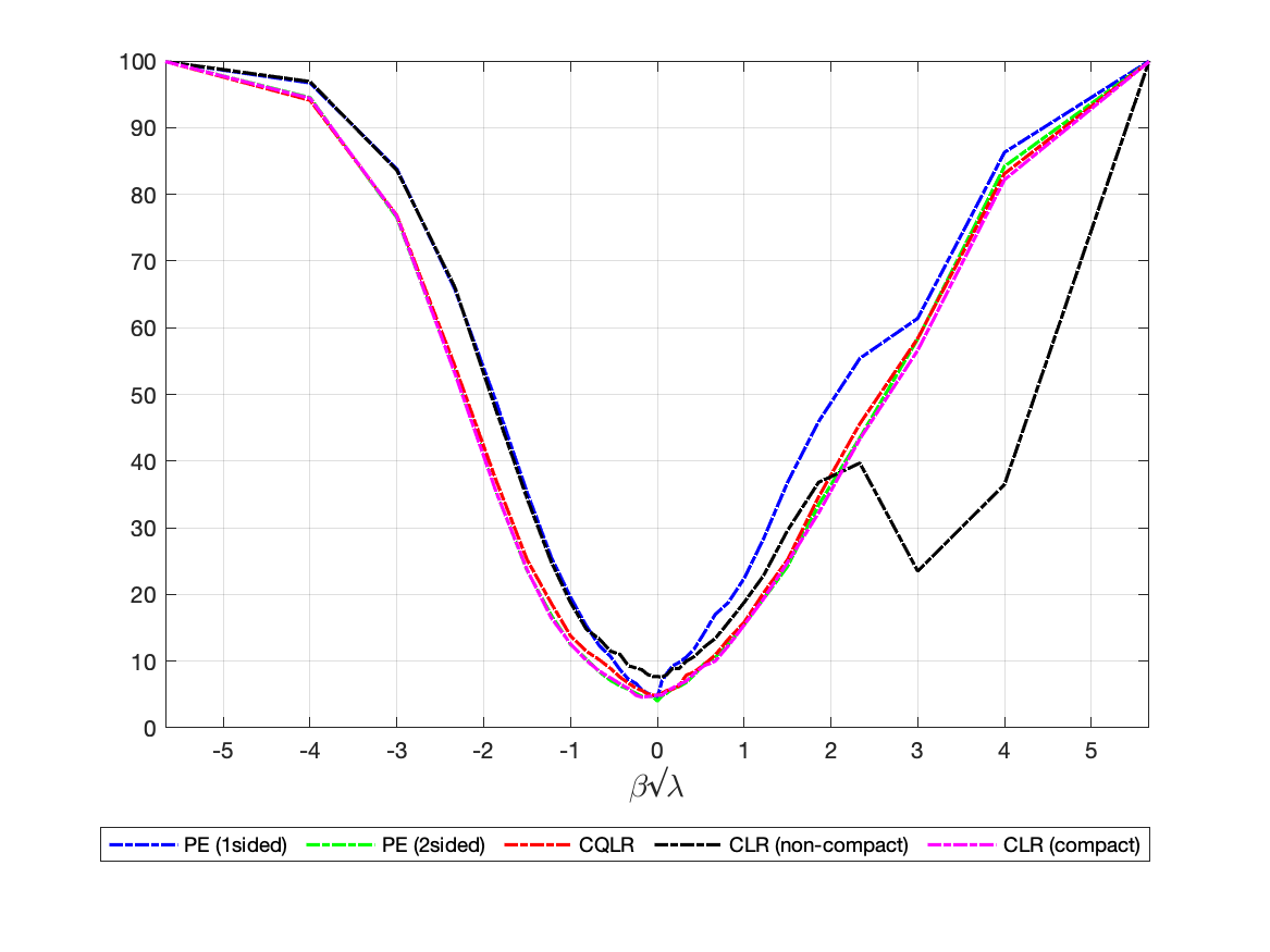
(a) $\rho=0.9$

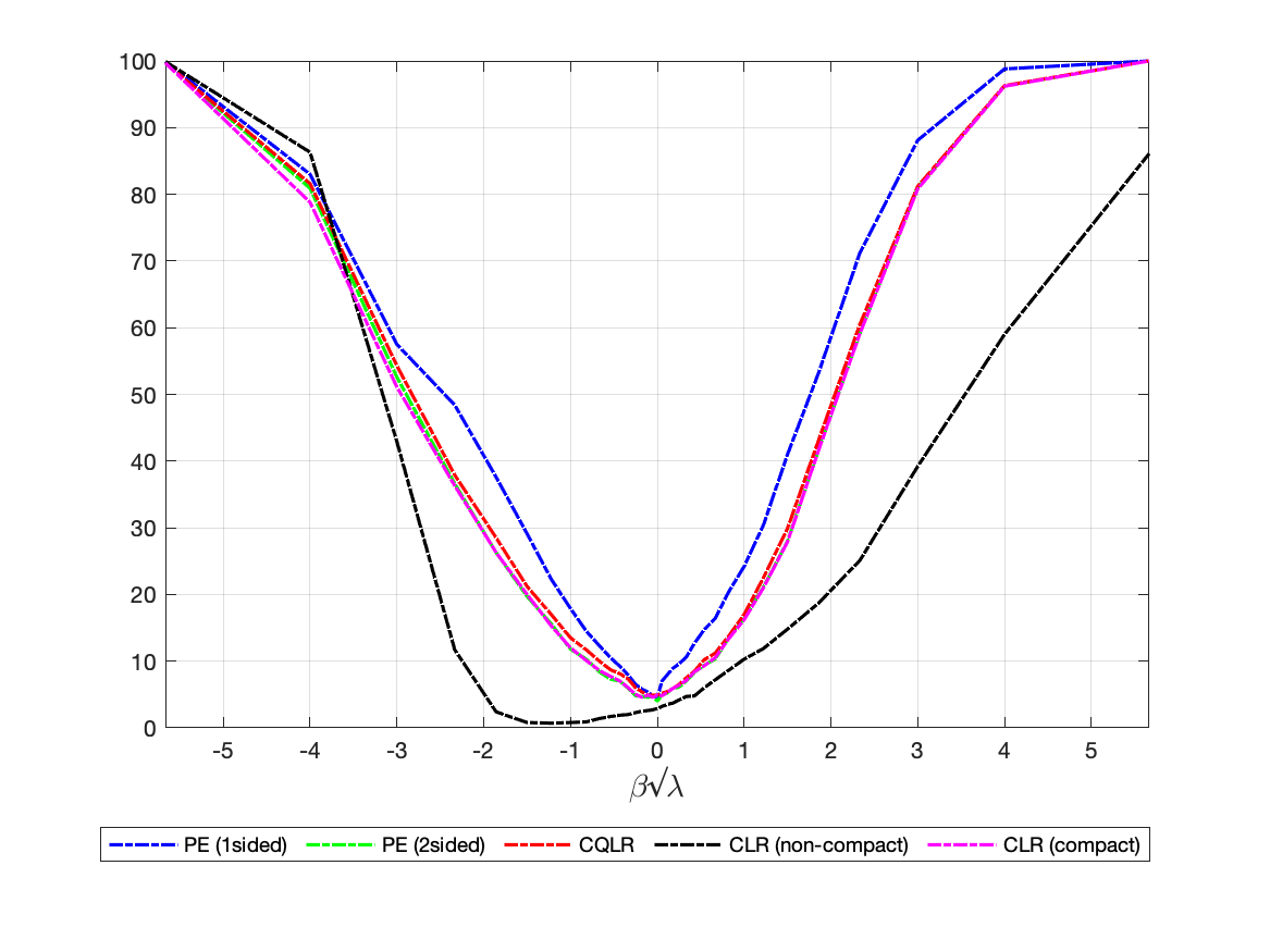
(b) $\rho=-0.9$

Figure 1 presents the one-sided and two-sided power envelope for invariant similar tests. These power envelopes are derived analytically by Mills, Moreira, and Vilela (2014) and Andrews, Moreira, and Stock (2006), respectively; see earlier theory by Andrews, Moreira, and Stock (2004). This early work also shows these power bounds are valid for all invariant tests which have correct size. We also plot power curves for the CQLR test as well as two numerical optimization strategies to obtain the CLR test. The first randomly draws the initial point for the search optimization algorithm in (2.20) for $\beta$. Here, we consider the uniform distribution over $\left[-1000,1000\right]$. The second one relies on the fact that we can maximize the likelihood over a compact set, without loss of generality. We can write the likelihood ratio statistic as

$$LR=\max_{\theta}vec(R)^{\prime}\Sigma^{-1/2}N_{\Sigma^{-1/2}(l_{\theta}\otimes I_{k})}\Sigma^{-1/2}vec(R)-T^{\prime}T,$$ (4.1)

where the maximization is over the compact set $\left[-pi/2,pi/2\right]$. The initial point is drawn from a uniform distribution over that same set. Recall that the CQLR and CLR tests are theoretically identical when errors are homoskedastic. Any power difference between the CQLR test and these numerical implementations for the CLR test arises from failures in the likelihood optimization.

The power upper bounds are useful to understand the difficulty in the likelihood optimization behind the CLR test. Both CQLR and CLR tests based on optimization over the compact set for $\theta$ perform alike. These two tests have power very close to the two-sided power envelope. The CLR test based on a draw-and-search for the optimal $\beta$ fails remarkably. In the first graph, this implementation has power above the two-sided power envelope and close to the one-sided power bound for parts of the parameter space. Furthermore, this implementation must fail to deliver a test with correct size. Indeed, the implementation for the CLR test over the whole real line has size close to 10% instead of the correct 5% level. To make matters even worse, the second plot in Figure 1 shows bad behavior associated with the sample implementation of the CLR test. The power can even be close to zero for parts of the parameter space.

Of course, one could simply use the CQLR test for the homoskedastic case. The lesson learned here is that likelihood optimization does matter for the power performance of the CLR test in general. In more complex designs (i.e., non-Kronecker error variance), drawing a unique initial point is far from sufficient. Our experience is that likelihood maximization for the implementation of the CLR test can be very slow and unreliable. This is particularly true when several initial points are required, as happens in some designs below.

Figure 2: Power Curves for Homoskedastic Errors and $k=5$
(Integrated Likelihood)

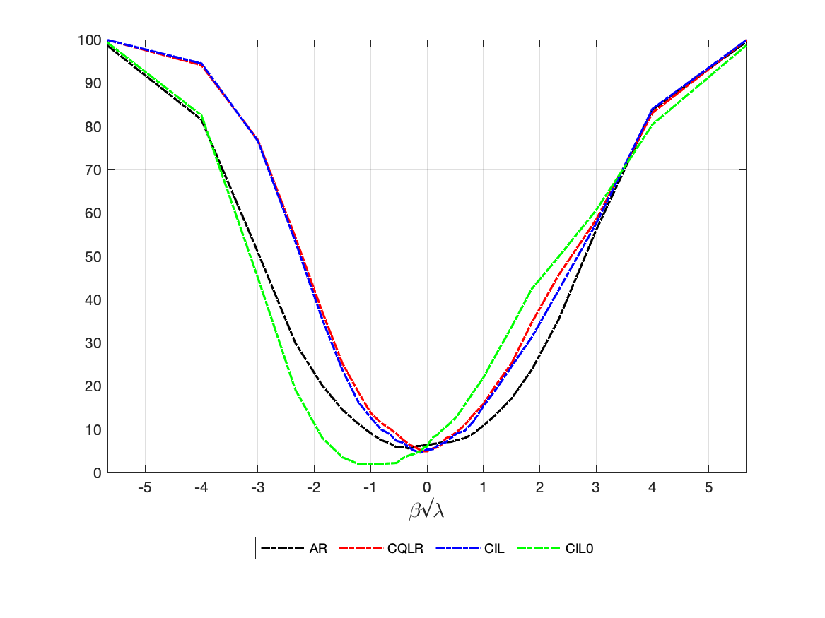
(a) $\rho=0.9$

(b) $\rho=-0.9$

Figure 2 presents power for the AR, CQLR, CIL, and CIL₀ tests. The CQLR and CIL tests have comparable power and outperform the AR test. These plots are a reassurance that the CIL test performs well in scenarios more favorable to CQLR. The CIL₀ test has behavior quite different from the CIL test. The dissimilar behavior of the CIL and CIL₀ tests illustrates that tests based on likelihood integration are sensitive to weight choices. While the CIL and CIL₀ tests perform comparably when $\lambda$ increases, they have distinct properties when IVs are weak. For one side of the alternative, the power of CIL₀ is smaller than that of the CQLR and CIL tests. For the other side of the alternative, it actually has larger power. Therefore, the CIL₀ behaves as a one-sided test. The CIL₀ test being biased means the null rejection probability is smaller for some alternatives than under the null. This undesirable feature of the CIL₀ test is not shared by the CQLR and CIL test. These two tests do not suffer the same power deficiencies as the CIL₀ test. They behave as two-sided tests by construction, and have power close to the power upper bound.

We now move to the more complex case in which errors can be heteroskedastic, autocorrelated, and/or clustered (HAC). We replicate four designs: the near-singular (NS), a variation thereof (NS with perturbation), and growing alternative (GA) designs of Moreira and Ridder (2020), and the non-Kronecker (NK) design of Moreira and Moreira (2019). While these simulations are not exhaustive for all parameter combinations, none of these designs is chosen to favor the CIL test over the CLR test. The main goal of these designs is only to show that there exist invariant tests which depend on the statistic $S$ beyond $AR$ and $LM$.

Table 1: Likelihood Optimization and Initial Values (percentage)

	(1,No)	(0,Yes)	(51,No)	(50, Yes)
(1,No)	-	64.7	86.7	87.7
(0,Yes)	26.0	-	47.1	47.2
(51,No)	0.1	3.5	-	4.2
(50,Yes)	0.1	-	0.4	-

To conserve space, we focus here only on simulations based on the NS design for $k=5$. We set $\mu=\lambda^{1/2}e_{1}$, with $\lambda/k=2$. For the variance matrix, we define $J_{k}$ to be the $k\times k$ matrix with the anti-diagonal elements equal to one and the other components zero. We have $J_{k}^{2}=I_{k}$. The $k\times k$ submatrices of $\Sigma_{0}$ are

$$\Sigma_{11}=c_{11}I_{k}\text{, }\Sigma_{12}=c_{12}J_{k}\text{, and }\Sigma_{22}=c_{22}I_{k}\text{,}$$ (4.2)

where $c_{11}$, $c_{12}$, and $c_{22}$ are tuning parameters. The values for the NS design are $c_{11}=1$, $c_{12}=100$, and $c_{22}=c_{12}^{2}+c_{12}^{-3}$. In this design, the power of both LM and CQLR tests is essentially equal to size. The full set of results for $k=2,5,10$ and $\lambda/k=2,10$ for all four designs, as well as descriptions of the NS with perturbation, GA, and NK designs, are presented in the supplement.

Table 2: Likelihood Optimization and Initial Values (factor)

	(1,No)	(0,Yes)	(51,No)	(50, Yes)
(1,No)	-	3,270.1	5,446.5	5,410.0
(0,Yes)	964.9	-	9,910.7	9,890.0
(51,No)	1,114.7	452.6	-	379.1
(50,Yes)	0.2	-	7.7	-

When the variance matrix has a Kronecker product form, the $LR$ statistic has a closed-form solution, and the CLR test reduces to the CQLR test. This sidesteps the daunting task of numerically optimizing the likelihood. In the special case with homoskedastic errors, choosing only one initial point after compactifying the search set is enough for our purposes. Unfortunately, this conclusion is not valid for more complex variance matrices. Table 1 assesses improvements for the likelihood optimization under the null hypothesis. The values inside the parentheses indicate the number of random initial points for $\theta$ and whether $\beta_{0}$ is included or not, respectively. We compute the LR statistic over 1,000 simulations for each case. We then report the proportion of times in which one setup outperforms another setup (relative improvement by an error margin of at least 0.1%).

Each row in Table 1 corresponds to a choice of the number of starting values and whether $\beta_{0}$ is among the starting values, as specified in the row header. The entries in a row report the fraction of repetitions in which the initial values selection and the inclusion of $\beta_{0}$, as specified in the column header, give a higher maximum likelihood value. For example, if we choose $\beta_{0}$ instead of only one random point as the initial value, we see improvements in the likelihood optimization 64.7% of the time. Conversely, the likelihood optimization performs better 26.0% of the time if we choose a random point instead of $\beta_{0}$. For both of these scenarios, improvements are gained by adding about 50 random initial values. This can be seen in the upper-right $2\times 2$ block in Table 1, where the improvements range from 47.1% to 87.7%. On the other hand, the improvements are negligible from starting with 50 random points and $\beta_{0}$ as initial values –even when we include 51 other random points. What is perhaps interesting is the improvement of 3.5% from adding $\beta_{0}$ as an initial value in addition to the 50 random points. These two findings suggest that running optimization algorithms after including 50 random points and $\beta_{0}$ as initial values should suffice for our purposes. More worrisome, for smaller values of $\lambda$ or other combinations of $\mu$ and the variance matrix, we may need to include even more initial points. This may happen, for example, if the likelihood can be flat for parts of the parameter space.

Table 2 presents the average percentage improvement (for the observations in which the error margin is at least 0.1%). Even when we include 51 random initial points, meaningful improvements can be gained by including the unknown parameter $\beta$. These gains are on the order of 379.1% for 4.2% of the replications when we include another 50 random initial points and $\beta$ itself. On the other hand, when we include 51 other random initial points beyond $\beta$ and 50 points, the average improvement is on the order of 7.7% for only 0.4% of the repetitions.

All simulations are for the null hypothesis. For the alternative, it is natural to use 50 random points, the null $\beta_{0}$, and the alternative $\beta$ as initial points. Of course, the parameter $\beta$ is unknown. However, we want to minimize the numerical issues associated with the CLR test, in case better optimization methods are found in the future. The table shows that the solution of using $\beta$ in addition to 50 random points works well to compute the LR statistic. A more complex problem happens when we find the approximation for the critical value function. Recall that this function is the conditional quantile under the null hypothesis. This quantile is found by generating $S$ from a standard multivariate normal distribution. That means the model is misspecified when $T$ is not generated under the null. One possibility is to use the pseudo-parameter which minimizes the Kullback-Leibler divergence criterion. This strategy follows from the fact that the maximum likelihood (ML) estimator converges to this pseudo-parameter under strong instruments. This route seems complicated and unnecessary for our purposes. Excluding this parameter, we get smaller values for the test statistic –not larger. Hence, the 95% quantile used for the critical value function tends to underestimate the true conditional quantile. The bottom line is that by including $\beta$, the $LR$ statistic is optimized properly while the conditional quantile can be smaller than it should be. This means that, if anything, we may be overestimating the power of the CLR test.

Finally, we evaluate improvements over other numbers of random initial points for $\theta$. For example, unreported simulations show gains of about 5.3% obtained from adding 1 initial random point beyond 20 random initial points. The choice of 50 seems the most sensible, in terms of reliability and computational speed. Even then, the computation time for CLR is about 35 times slower than that of the CIL test, on average (with the range between 4 to 100 times slower). For the aforementioned reasons, we include $\beta_{0}$ and $\beta$ as initial points as well. At least for the designs considered here, unreported power comparisons for different choices of initial values indicate that including 50 random points, $\beta_{0}$, and $\beta$ offers stable and reliable power curves. There is, of course, no guarantee that this searching scheme would be sufficient for other designs.

Figure 3: Power Curves for HAC Errors with $k=5$ and $\lambda/k=2$

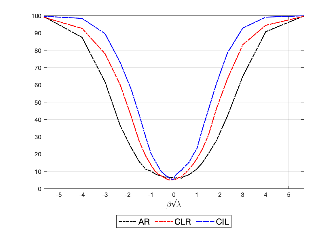
(a) NS Design

(b) NS with perturbation

(c) GA Design

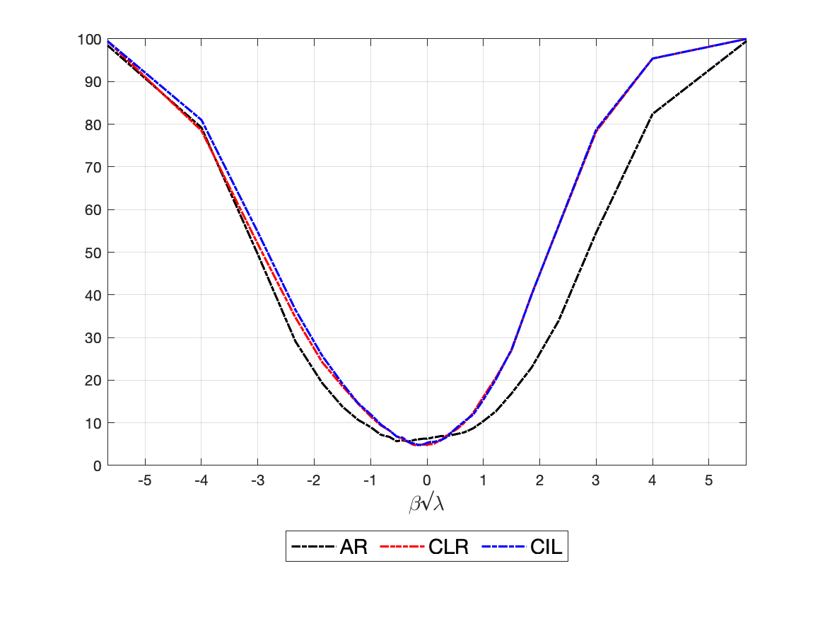
(d) NK Design

We now briefly discuss power. More extensive power comparisons are reported in the supplement (due to computational time for the CLR, these additional comparisons use only 200 Monte Carlo replications for power and 200 simulations for conditional quantiles). Figure 3 presents power for the AR, CLR, CIL, and CIL₀ tests when $k=5$ and $\lambda/k=2$. We consider all four sets of simulations: NS design, NS design with a perturbation, GA design, and NK design. As before, the CIL₀ test can be biased, while the CLR and CIL tests dominate the AR test. In general, the CIL test outperforms the CLR test. The power difference can be as large as 15% for these specific designs. For example, the CIL test can have power near 85% when the CLR test rejects the null about 70% of the time. This difference happens even when we implement the infeasible version of the CLR test which includes $\beta$ as one of the initial points.

The more technical sections of the paper are next. Section 5 builds upon and connects with the work of AMS06. Section 6 derives the CIL test.

5 Kronecker Variance Matrix

We first consider the special case where $\Sigma=\Omega\otimes\Phi$ with $\Omega$ a $2\times 2$ matrix and $\Phi$ a $k\times k$ matrix. The Kronecker product framework is particularly interesting for two reasons. First, we find the maximal invariant, taking into consideration a transformation of $\Omega$ which is known but not fixed. This yields the same data reduction from $S$ and $T$ as that obtained by AMS06 under the assumption that $\Omega$ is known and fixed. This result is striking as the AMS06 approach does not hold for general $\Sigma$, but ours does. Second, AMS06 do not rule out the possibility that the test depends on $\Omega$ beyond the statistics $S$ and $T$, because AMS06 treat $\Omega$ as being fixed. Our framework instead shows that invariant tests should not depend on $\Omega$ at all.

The $S$ and $T$ statistics in (2.11) simplify to the original statistics of Moreira (2002, 2009) and AMS06 for the homoskedastic model. When $\Sigma=\Omega\otimes\Phi$, the statistics $S$ and $T$ become

$$S = \Phi^{-1/2}(Z^{\prime}Z)^{-1/2}Z^{\prime}Yb_{0}\cdot(b_{0}^{\prime}\Omega b_{0})^{-1/2}\text{ and }$$ (5.1)

$$T = \Phi^{-1/2}(Z^{\prime}Z)^{-1/2}Z^{\prime}Y\Omega^{-1}a_{0}\cdot(a_{0}^{\prime}\Omega^{-1}a_{0})^{-1/2}.$$

Their distribution is given by

$$S\sim N\left(c_{\beta}\Phi^{-1/2}\mu,I_{k}\right)\text{ and }T\sim N\left(d_{\beta}\Phi^{-1/2}\mu,I_{k}\right)$$ (5.2)

with $c_{\beta}=(\beta-\beta_{0})\cdot(b_{0}^{\prime}\Omega b_{0})^{-1/2}$ and $d_{\beta}=a^{\prime}\Omega^{-1}a_{0}\cdot(a_{0}^{\prime}\Omega^{-1}a_{0})^{1/2}$. AMS06 develop the theory of invariant tests by treating $\Omega$ as known and fixed. Even if $\Phi$ is known, the parameter $\mu_{\Phi}=\Phi^{-1/2}\mu$ is unknown, because $\mu$ is unknown. Hence, AMS06’s invariance argument applies to the new parameter $\mu_{\Phi}=\Phi^{-1/2}\mu$. Specifically, let $h_{1}\in\mathcal{O}\left(k\right)$, the group of orthogonal matrices with matrix multiplication as the group operator. The corresponding transformation in the sample space is

$$h_{1}\circ\left[S:T\right]=h_{1}\cdot\left[S:T\right].$$ (5.3)

The associated transformation in the parameter space is

$$h_{1}\circ\left(\beta,\mu_{\Phi}\right)=\left(\beta,h_{1}.\mu_{\Phi}\right).$$ (5.4)

The transformation does not change $\beta$, so our testing problem is preserved. As argued before, this means that the test statistic should be an invariant statistic (under the transformation $h_{1}$).

The maximal invariant statistic for the orthogonal transformation is

$$Q=\left[\begin{array}[]{cc}Q_{S}&Q_{ST}\\ Q_{ST}&Q_{T}\end{array}\right]=\left[\begin{array}[]{cc}S^{\prime}S&S^{\prime}T\\ S^{\prime}T&T^{\prime}T\end{array}\right].$$ (5.5)

That is, any invariant test depends on the data only through $Q$. The density of $Q$ at $q$ for the parameters $\beta$ and $\lambda=\mu_{\Phi}^{\prime}\mu_{\Phi}$ is given by

$$f_{\beta,\lambda}(q_{S},q_{ST},q_{T})\overset{}{=}K_{0}\exp(-\lambda(c_{\beta}^{2}+d_{\beta}^{2})/2)\left|q\right|^{(k-3)/2}$$ (5.6)

$$\hskip 74.438pt\times\exp(-(q_{S}+q_{T})/2)(\lambda\xi_{\beta}(q))^{-(k-2)/4}I_{(k-2)/2}(\sqrt{\lambda\xi_{\beta}(q)}),$$

where $K_{0}^{-1}=2^{(k+2)/2}pi^{1/2}\Gamma_{(k-1)/2}$, $\Gamma_{(\cdot)}$ is the gamma function, $I_{(k-2)/2}(\cdot)$ denotes the modified Bessel function of the first kind, and

$$\xi_{\beta}(q)=c_{\beta}^{2}q_{S}+2c_{\beta}d_{\beta}q_{ST}+d_{\beta}^{2}q_{T}.$$ (5.7)

AMS06 further shows that another group, given by sign transformations, preserves $H_{0}:\beta=\beta_{0}$ against $H_{0}:\beta\neq\beta_{0}$. Consider the group $\mathcal{O}\left(1\right)$, which contains only two elements: $h_{2}\in$ $\left\{-1,1\right\}$. For $h_{2}=-1$, the data transformation is given by

$$h_{2}\circ\left[S:T\right]=\left[-S:T\right]$$ (5.8)

(by the definition of a group, the parameter remains unaltered at $h_{2}=1$). This yields a transformation in the maximal invariant space for $h_{2}$:

$$h_{2}\circ\left(Q_{S},Q_{ST},Q_{T}\right)=\left(Q_{S},h_{2}Q_{ST},Q_{T}\right).$$ (5.9)

The maximal invariant for the joint transformation $h=\left(h_{1},h_{2}\right)$ is the vector with components $Q_{S}$, $Q_{ST}^{2}$, and $Q_{T}$. In principle, the tests can depend on $\Omega$ with homoskedastic errors. As we will see in Theorem 2, we are able to eliminate the dependence on the variance as well, and show the triad $Q_{S}$, $Q_{ST}^{2}$, and $Q_{T}$ is the maximal invariant for $g=\left(g_{1},g_{2}\right)$ in the case of known, but not fixed, variance.

5.1 Instrument Transformation

The orthogonal transformation argument of AMS06 is originally designed for homoskedastic errors. For the general Kronecker case, both $\Phi^{1/2}S$ and $\Phi^{1/2}T$ (which are equivalent to the original statistics of AMS06) have variance $\Phi$. Because their methodology assumes the variance to be fixed, their orthogonal transformation would not work, in general, because the variance would change. We could manually standardize their statistics by $\Phi^{-1/2}$ to obtain our statistics $S$ and $T$, and apply the orthogonal group, as done earlier. An alternative solution is to allow $\Phi$ to be known, but for it to change as we transform the data. For example, take the special case in which $\Phi$ is a diagonal matrix. If we were to permute the entries of $S$ and $T$ jointly, perhaps we should allow the permutation of the diagonal entries of $\Phi$ as well. Formally, we will take the variance $\Sigma=\Omega\otimes\Phi$ as part of both data and parameter spaces.

For the special case in which $\Sigma=\Omega\otimes\Phi$, the distribution of $R_{0}$ is given by

$$R_{0}\sim N\left(\mu\left(\Delta,1\right),\Omega_{0}\otimes\Phi\right),$$ (5.10)

where $\Delta=\beta-\beta_{0}$, $\Sigma_{0}=\Omega_{0}\otimes\Phi$, and $\Omega_{0}=B_{0}^{\prime}\Omega B_{0}$. The data are the realizations $(R_{0},\Omega_{0},\Phi)$ and the parameters are $(\Delta,\mu,\Omega_{0},\Phi)$. The matrices $\Omega_{0},\Phi$ are assumed to be known, but not fixed. Thus, $\Omega_{0},\Phi$ are both parameters and part of the data, simultaneously.

We introduced the $g_{1}\in G_{L}\left(k\right)$ transformation in Section 3.1. Its action on the sample space is given by

$$g_{1}\circ\left(R_{0},\Omega_{0},\Phi\right)=\left(g_{1}R_{0},\Omega_{0},g_{1}\Phi g_{1}^{\prime}\right).$$ (5.11)

We note that

$$g_{1}R_{0}\sim N\left(g_{1}\mu\left(\Delta,1\right),\Omega_{0}\otimes g_{1}\Phi g_{1}^{\prime}\right),$$ (5.12)

so the corresponding action on the parameter space is

$$g_{1}\circ\left(\Delta,\mu,\Omega_{0},\Phi\right)=\left(\Delta,g_{1}\mu,\Omega_{0},g_{1}\Phi g_{1}^{\prime}\right).$$ (5.13)

We now show that the matrix

$$Q=\left[S:T\right]^{\prime}\left[S:T\right]=\left[\begin{array}[]{cc}S^{\prime}S&S^{\prime}T\\ S^{\prime}T&T^{\prime}T\end{array}\right],$$ (5.14)

together with $\Omega_{0}$ itself, is the maximal invariant statistic. That is, any other invariant statistic can be written as a function of $\left(Q,\Omega_{0}\right)$. The distribution of the maximal invariant depends only on the concentration parameter $\lambda$, the parameter of interest $\beta$, and $\Omega_{0}$ itself.

Theorem 1.

For the group actions in (5.11) and (5.13):
(i) The maximal invariant in the sample space is given by $\left(Q,\Omega_{0}\right)$; and
(ii) The maximal invariant in the parameter space is given by $\left(c_{\beta}^{2}\lambda,c_{\beta}d_{\beta}\lambda,d_{\beta}^{2}\lambda,\Omega_{0}\right)$.

Comments: 1. The data $\left(\left[S:T\right],\Omega_{0},\Phi\right)$ is a one-to-one transformation from the primitive data $\left(R,\Omega,\Phi\right)$. Hence, there is no loss of generality in using the pivotal statistic $S$ and the complete statistic $T$ instead of using $R$ (or $R_{0}$).

2. There is a one-to-one mapping between $\Omega_{0}$ and $\Omega$. Hence, $\left(Q,\Omega\right)$ is a maximal invariant as well. We continue to use $\Omega_{0}$ because it is useful to find a maximal invariant for the two-sided transformations to be considered next.

3. The statistic $Q$ is the maximal invariant based on the compact orthogonal group on $\left[S:T\right]$, which is a straightforward application of AMS06. We instead allow the much larger, noncompact group of nonsingular matrices with unitary determinant. The data also contain the variance components given by $\Omega_{0}$ and $\Phi$. Because the group $\mathcal{G}_{L}\left(k\right)$ is not amenable, the Hunt-Stein theorem is not applicable, and we do not necessarily obtain a minimax result. This is in contrast to Chamberlain (2007), who builds on the fact that the orthogonal group is compact.

4. The component $\Phi$ completely vanishes as the noncompact group $\mathcal{G}_{L}\left(k\right)$ acts transitively on $\Phi$. Hence, the matrix $\Phi$ is not part of the maximal invariant.

5.2 Two-Sided Transformation

We now apply the $g_{2}\in\mathcal{G}_{T}\left(2\right)$ transformation introduced in Section 3.1. The two-sided transformation in the Kronecker model is given by

$$g_{2}\circ\left(R_{0},\Omega_{0},\Phi\right)=\left(R_{0}g_{2}^{\prime},g_{2}\Omega_{0}g_{2}^{\prime},\Phi\right),$$ (5.15)

where $g_{2}\in\mathcal{G}_{T}\left(2\right)$, the group of nonsingular lower triangular $2\times 2$ matrices. The transformation in the parameter space is

$$g\circ\left(\Delta,\mu,\Sigma_{0}\right)=\left(\frac{\Delta g_{11}}{\Delta g_{21}+g_{22}},g_{1}\mu\left(\Delta g_{21}+g_{22}\right),\left(g_{2}\otimes g_{1}\right)\Sigma_{0}\left(g_{2}^{\prime}\otimes g_{1}^{\prime}\right)\right).$$ (5.16)

Theorem 2 finds the maximal invariant based on $g_{1}\in\mathcal{G}_{L}\left(k\right)$ and $g_{2}\in\mathcal{G}_{T}\left(2\right)$.

Theorem 2.

For the data group actions defined in (5.11) and (5.15), and the parameter actions in (5.13) and (5.16), we find
(i) The induced group action of $g_{2}$ on the space $\left(\left[S:T\right],\Omega_{0},\Phi\right)$ is

$$g_{2}\circ\left(\left[S:T\right],\Omega_{0},\Phi\right)=\left(\left[sgn\left(g_{11}\right)S:sgn\left(g_{22}\right)T\right],g_{2}\Omega_{0}g_{2}^{\prime},\Phi\right);$$

(ii) The data maximal invariant to $g=\left(g_{1},g_{2}\right)$ is

$$\left(Q_{S},Q_{T},Q_{ST}^{2}\right);$$

(iii) The induced group action by $g_{2}$ on the parameter functions $\left(c_{\beta},d_{\beta},\mu,\Omega_{0},\Phi\right)$ is given by

$$g_{2}\circ\left(c_{\beta}\mu,d_{\beta}\mu,\Omega_{0},\Phi\right)=\left(sgn\left(g_{11}\right)c_{\beta}\mu,sgn\left(g_{22}\right)d_{\beta}\mu,g_{2}\Omega_{0}g_{2}^{\prime},\Phi\right);\text{ and}$$

(iv) The parameter maximal invariant to $g=\left(g_{1},g_{2}\right)$ is

$$\left(c_{\beta}^{2}\lambda,d_{\beta}^{2}\lambda,\left|c_{\beta}d_{\beta}\right|\lambda\right).$$

Comments: 1. The parameters $\beta$ and $\Omega$ remain unchanged by the action (5.13). Because the parameters $c_{\beta}$ and $d_{\beta}$ depend only on $\beta$ and $\Omega$, they are preserved as well. The result now follows trivially because $g_{1}\circ\left(\mu,\Omega,\Phi\right)=\left(g_{1}\mu,\Omega,g_{1}\Phi g_{1}^{\prime}\right)$.

2. We note that $g_{21}$ may be different from zero. Hence, the group of transformations is larger than scale multiplication to each entry of the vector $\left(\Delta,1\right)$. A naive generalization for the sign group of transformations by AMS06 to our setup is a diagonal matrix $g_{2}$. In the online appendix, we show that some invariant tests based on the associated maximal invariant can behave as one-sided tests. Hence, we illustrate the importance of finding the largest group of transformations before deriving invariant tests.

These actions are defined using the reduced-form matrix $\Omega$. For the homoskedastic model, we could analyze the transformations in the structural-form matrix

$$\Psi=\left[\begin{array}[]{cc}\sigma_{uu}&\sigma_{u2}\\ \sigma_{u2}&\sigma_{22}\end{array}\right].$$ (5.17)

One may wonder if there are actually symmetries in the original model. This turns out to be true. In fact, the action in the structural-form variance matrix has a very simple structure.

Proposition 1.

The group action on the reduced-form matrix $\Omega$ induces an action on the structural-form matrix $\Psi$:

$$g_{2}\circ\left(\Delta,\lambda,\Psi\right) = \left(\frac{\Delta g_{11}}{\Delta g_{21}+g_{22}},\left(\Delta g_{21}+g_{22}\right)^{2}\lambda,\Gamma\Psi\Gamma^{\prime}\right)\text{, where}$$

$$\Gamma = \left[\begin{array}[]{cc}\left(\Delta g_{21}+g_{22}\right)^{-1}g_{11}g_{22}&0\\ g_{21}&\Delta g_{21}+g_{22}\end{array}\right].$$

Comment: Take $\beta_{0}=0$. When $g_{11}=-1,$ $g_{21}=0,$ and $g_{22}=1$, we have $g_{2}\circ\left(v_{1},v_{2}\right)=\left(-v_{1},v_{2}\right)$. Therefore, $\sigma_{11}$ and $\sigma_{22}$ are preserved while $\sigma_{12}$ changes sign. Since $\sigma_{12}=\sigma_{u2}+\sigma_{22}\beta$, the new value for the structural-form covariance scalar, $-\sigma_{u2}$, and the new value of the parameter, $-\beta$, comprise the only transformation that works for any value of $\sigma_{22}$.

A corollary of our theory is that the AR test is UMPI when structural-form variance is fixed. This optimality result is novel and important. All optimality theorems for the AR test, so far, assume the reduced-form variance to be fixed (Moreira (2002, 2009), AMS06, and Moreira and Moreira (2019)).

6 Invariant Tests

We now use the group of transformations by $g=\left(g_{1},g_{2}\right)$ to develop the CIL test. Recall that the data consist of $R_{0}$ and $\Sigma_{0}$, where $R_{0}$ has a normal distribution and the distribution of $\Sigma_{0}$ is degenerate. So, the density of the data is the product of two parts. The first part is the normal distribution of $R_{0}$, which is absolutely continuous with respect to the Lebesgue measure. The second part is the degenerate distribution of $\Sigma_{0}$, which is absolutely continuous with respect to the counting measure. Understanding how the density changes with the data transformation is important for the development of the CIL test.

The density of $R_{0}=\left[R_{1}:R_{2}\right]$ evaluated at $r_{0}=\left[r_{1}:r_{2}\right]$ is given by

$$f_{R}\left(r_{0};\Delta,\mu,\Sigma_{0}\right)=\left(2pi\right)^{-k}\left|\Sigma_{0}\right|^{-1/2}\exp\left\{-\frac{1}{2}\left[\begin{array}[]{c}r_{1}-\mu\Delta\\ r_{2}-\mu\end{array}\right]^{\prime}\Sigma_{0}^{-1}\left[\begin{array}[]{c}r_{1}-\mu\Delta\\ r_{2}-\mu\end{array}\right]\right\}.$$ (6.1)

As in Theorem 2, we consider the groups of instrument transformations $g_{1}$ and two-sided transformations $g_{2}$ together, so that we have the joint transformation $g=\left(g_{1},g_{2}\right)$ defined in Section 3.1, where $g_{1}\in\mathcal{G}_{L}\left(k\right)$ and $g_{2}\in\mathcal{G}_{T}\left(2\right)$, and the associated transformation $g\circ\left(\Delta,\mu,\Sigma_{0}\right)$ in the parameter space.

Basic algebraic manipulations show that

$$f_{R}\left(g\circ r_{0};g\circ\left(\Delta,\mu,\Sigma_{0}\right)\right)=f_{R}\left(\left[r_{1}:r_{2}\right];\Delta,\mu,\Sigma_{0}\right)\left|g_{2}\right|^{-k}\left|g_{1}\right|^{-2}$$ (6.2)

because

$$\left|\left(g_{2}\otimes g_{1}\right)\Sigma_{0}\left(g_{2}^{\prime}\otimes g_{1}^{\prime}\right)\right|=|g_{2}|^{2k}|g_{1}|^{4}|\Sigma_{0}|.$$ (6.3)

Therefore,

$$f_{R}\left(r_{0};\Delta,\mu,\Sigma_{0}\right)=f_{R}\left(g\circ r_{0};g\circ\left(\Delta,\mu,\Sigma_{0}\right)\right)\chi_{0}\left(g\right),$$ (6.4)

where $\chi_{0}\left(g\right)=\chi_{1}\left(g_{1}\right)\chi_{2}\left(g_{2}\right)$ for the sub-group multipliers $\chi_{1}\left(g_{1}\right)=\left|g_{1}\right|^{2}$ and $\chi_{2}\left(g_{2}\right)=\left|g_{2}\right|^{k}$. Hence, the density of $R_{0}$ is relatively invariant with multiplier $\chi_{0}(g)$.

Of course, the action $g\in\mathcal{G}_{L}\left(k\right)\times\mathcal{G}_{T}\left(2\right)$ is not proper. We can impose $\left|g_{1}\right|=1$ so that $\chi_{1}\left(g_{1}\right)=1$. In this case, $g_{1}\in\mathcal{S}_{L}\left(k\right)$, the group of invertible matrices with determinant equal to one. Alternatively, we can use another standardization such as $g_{22}=1$. To develop the integrated likelihood invariant test, we use Haar measures to obtain invariant tests. It is harder to work with the Haar measure for $\mathcal{S}_{L}\left(k\right)$ than for $\mathcal{G}_{L}\left(k\right)$; see Dedić (1990). On the other hand, it is relatively simple to derive the Haar measure for $2\times 2$ lower triangular matrices with $g_{22}=1$. For this reason, we prefer to impose a restriction on $\mathcal{G}_{T}\left(2\right)$.

For the second part, the data $\Sigma_{0}$ have a distribution that assigns probability one to the value $\Sigma_{0}$ itself. Therefore, the density at some arbitrary matrix value $\sigma_{0}$ is

$$f_{\Sigma}\left(\sigma_{0};\Sigma_{0}\right)=P_{\Sigma_{0}}\left(\sigma_{0}=\Sigma_{0}\right)=I\left(\sigma_{0}=\Sigma_{0}\right).$$ (6.5)

Using (6.5), we have

$$f_{\Sigma}(g\circ\sigma_{0};g\circ\Sigma_{0})=f_{\Sigma}\left(\left(g_{2}\otimes g_{1}\right)\sigma_{0}\left(g_{2}^{\prime}\otimes g_{1}^{\prime}\right);\left(g_{2}\otimes g_{1}\right)\Sigma_{0}\left(g_{2}^{\prime}\otimes g_{1}^{\prime}\right)\right)=f_{\Sigma}\left(\sigma_{0};\Sigma_{0}\right)$$ (6.6)

so that this density is invariant with multiplier 1.

The joint likelihood is then given by

$$f\left(r_{0},\sigma_{0};\Delta,\mu,\Sigma_{0}\right)=f_{R}\left(r_{0};\Delta,\mu,\Sigma_{0}\right)\cdot f_{\Sigma}\left(\sigma_{0};\Sigma_{0}\right),$$ (6.7)

so that

$$f\left(r_{0},\sigma_{0};\Delta,\mu,\Sigma_{0}\right)=f\left(g\circ\left(r_{0},\sigma_{0}\right);g\circ\left(\Delta,\mu,\Sigma_{0}\right)\right)\cdot\chi_{0}\left(g\right),$$ (6.8)

i.e. the likelihood is relatively invariant with multiplier $\chi_{0}(g)$. Because the Lebesgue measure is relatively left invariant for the group $g$ with multiplier $\chi_{0}(g)$, the (relative) invariance of the likelihood follows directly.

We use the invariance of the likelihood to propose a conditional weighted likelihood ratio test. We also show that the AR, LM, CQLR, and CLR tests are also invariant.

6.1 Optimal Tests

Our goal in this section is to find optimal tests. Specifically, a test is defined to be a measurable function $\phi\left(r_{0},\sigma_{0}\right)$ that is bounded by $0$ and $1$. For a given outcome, the test rejects the null with probability $\phi\left(r_{0},\sigma_{0}\right)$ and accepts the null with probability $1-\phi\left(r_{0},\sigma_{0}\right)$, e.g., the Anderson-Rubin test is simply $I\left(AR>c\left(k\right)\right)$ where $I\left(\cdot\right)$ is the indicator function. The test is said to be nonrandomized if $\phi$ takes only values $0$ and $1$; otherwise, it is called a randomized test. The rejection probability is given by

$$E_{\Delta,\mu,\Sigma_{0}}\phi\left(R_{0},\Sigma_{0}\right)\equiv\int\phi\left(r_{0},\sigma_{0}\right)f\left(r_{0},\sigma_{0};\Delta,\mu,\Sigma_{0}\right)\text{ }dr_{0}\text{ }\eta\left(d\sigma_{0}\right),$$ (6.9)

where $\eta$ is the counting measure. The rejection probability (6.9) simplifies to

$$E_{\Delta,\mu,\Sigma_{0}}\phi\left(R_{0},\Sigma_{0}\right) = \int\phi\left(r_{0},\sigma_{0}\right)f_{R}\left(r_{0};\Delta,\mu,\Sigma_{0}\right)f_{\Sigma}\left(\sigma_{0};\Sigma_{0}\right)\text{ }dr_{0}\text{ }\eta\left(d\sigma_{0}\right)$$ (6.10)

$$= \int\phi\left(r_{0},\Sigma_{0}\right)f_{R}\left(r_{0};\Delta,\mu,\Sigma_{0}\right)\text{ }dr_{0}.$$

The rejection probability $E_{\Delta,\mu,\Sigma_{0}}\phi\left(R_{0},\Sigma_{0}\right)$ taken as a function of $\Delta$, $\mu$, and $\Sigma_{0}$ gives the power curve for the test $\phi$. In particular, $E_{0,\mu,\Sigma_{0}}\phi\left(R_{0},\Sigma_{0}\right)$ gives the null rejection probability.

Let the parameter space for $\Delta,\mu,\sigma_{0}$ be denoted by $\Theta$, with $\sigma$-field the intersection of $\Theta$ and sets in $\mathcal{B}^{k+1}\times\{\Sigma_{0}\}$. Let $w$ be a measure on that $\sigma$-field. We average the power curve over the parameter space to obtain the weighted average power with weights that are given by the measure $w$. By Tonelli’s theorem, the weighted average power is

$$E_{w}\phi\left(R_{0},\Sigma_{0}\right)=\int E_{\Delta,\mu,\Sigma_{0}}\phi\left(R_{0},\Sigma_{0}\right)dw\left(\Delta,\mu,\Sigma_{0}\right).$$ (6.11)

If the weights are such that for $B\times\{\Sigma_{0}\}$,

$$w\left(B\times\{\Sigma_{0}\}\right)=w_{R}\left(B\right)\cdot w_{\Sigma}\left(\{\sigma_{0}\}\right),$$ (6.12)

where $B\in\mathcal{B}^{k+1}$ and $w_{\Sigma}\left(\{\sigma_{0}\}\right)$ has unitary mass on $\{\Sigma_{0}\}$, then

$$E_{w}\phi\left(R_{0},\Sigma_{0}\right)=\int\phi\left(r_{0},\Sigma_{0}\right)f_{w_{R}}\left(r_{0},\Sigma_{0}\right)\text{ }dr_{0},$$ (6.13)

where $f_{w_{R}}\left(r_{0},\Sigma_{0}\right)$ is defined as

$$f_{w_{R}}\left(r_{0},\Sigma_{0}\right)=\int f_{R}\left(r_{0};\Delta,\mu,\Sigma_{0}\right)\text{ }dw_{R}\left(\Delta,\mu\right).$$ (6.14)

For a given weight $w$, we seek optimal similar tests

$$\max_{0\leq\phi\leq 1}E_{w}\phi\left(R_{0},\Sigma_{0}\right)\text{, where }E_{0,\mu,\Sigma_{0}}\phi\left(R_{0},\Sigma_{0}\right)=\alpha,\forall\mu.$$ (6.15)

The next proposition finds the WAP test.

Proposition 2.

The optimal test in (6.15) rejects the null when

$$\frac{f_{w_{R}}\left(r_{0},\Sigma_{0}\right)}{f_{S}\left(s\right)}>\kappa\left(t,\Sigma_{0}\right),$$ (6.16)

where $f_{S}\left(s\right)=\left(2pi\right)^{-k/2}e^{-s^{\prime}s/2}$ is the density of the statistic $S$ under the null.

Comment: Because $T$ is sufficient for $\mu$ under the null, we condition on $T=t$. The dependence of the test statistic on $t$ is absorbed in the critical value of the test.

For arbitrary weights, the WAP similar test is not guaranteed to have overall good power in finite samples. In particular, the power can be near zero for parts of the parameter space (as happens with the CIL₀ test for $k>2$). We circumvent this problem by carefully choosing weights $w$ so that the test given by (6.16) is invariant. The CIL test behaves as a two-sided test, and so, it does not suffer the criticism by Moreira and Moreira (2019).

6.2 Similar Invariant Tests

Invariance of conditional tests follows from the relative invariance of test statistics.

Definition 1.

A statistic $\psi$ is relatively (left) invariant to $g$ with multiplier $\chi$ if

$$\psi\left(g\circ\left(s,t,\sigma_{0}\right)\right)=\chi\left(g\right)\cdot\psi\left(s,t,\sigma_{0}\right),$$

for any $\left(s,t,\sigma_{0}\right)$.

Proposition 3 establishes the invariance of the conditional test if the test statistic is relatively invariant.

Proposition 3.

Suppose that $\psi\left(S,t,\Sigma_{0}\right)$ is a continuous random variable under $H_{0}:\Delta=0$ for every $t$. Define $\kappa_{\psi}\left(t,\Sigma_{0}\right)$ to be the $1-\alpha$ quantile of the null distribution of $\psi\left(S,t,\Sigma_{0}\right)$. Then the following hold:
(i) The conditional test $\phi\left(s,t,\Sigma_{0}\right)$ that rejects the null when

$$\psi\left(s,t,\Sigma_{0}\right)>\kappa_{\psi}\left(t,\Sigma_{0}\right)$$

is similar at level $\alpha$;
(ii) If $\psi\left(g\circ\left(s,t,\Sigma_{0}\right)\right)$ is relatively invariant under $g\in\mathcal{G}_{L}\left(k\right)\times G_{T}\left(2\right)$ with multiplier $\chi$, then $\kappa_{\psi}\left(t,\Sigma_{0}\right)$ is itself relatively invariant with multiplier $\chi$; and
(iii) The conditional test $\phi\left(s,t,\Sigma_{0}\right)$ is invariant.

Comments: 1. Careful examination of the proof shows that invariance of the conditional quantile does not depend on the group transformation used. It is also applicable to other models as long as there is a sufficient statistic, e.g. here under the null, that is boundedly complete.

2. The comment above explains why the conditional quantile of the $LR$ statistic depends only on $T^{\prime}T$ in the homoskedastic case. The LR statistic does not depend on $\Omega_{0}$ at all, and $T^{\prime}T$ is the maximal invariant to orthogonal transformations $h_{1}\circ T=h_{1}\cdot T$. This is consistent with the results of Moreira (2003) and AMS06, but with no need to use pivotal statistics and independence.

Before showing that the CIL test is invariant and is the limit of conditional WAP tests, as given by (6.16), we establish that the $AR$, $LM$, $LR$, and $QLR$ statistics are invariant.

Proposition 4.

The $AR$, $LM$, $LR$, and $QLR$ statistics are invariant to $g=\left(g_{1},g_{2}\right)\in\mathcal{G}_{L}\left(k\right)\times\mathcal{G}_{T}\left(2\right)$.

Comment: Close inspection shows the proof of invariance of the $LR$ statistic is very general. It works for any model in the presence of symmetries which preserve the testing problem.

6.3 An Invariant WAP Similar Test

The goal is to obtain a WAP invariant similar test in the over-identified model ($k>1$). This entails finding weights so that the final test is relatively invariant.

Definition 2.

A measure $m$ is relatively (left) invariant with multiplier $\chi$ if

$$\int F\left(g^{-1}\circ\theta\right)m\left(d\theta\right)=\chi\left(g\right)\int F\left(\theta\right)m\left(d\theta\right)$$

for any real-valued continuous function $F$ with bounded support.

We could apply this result for $\theta=\left(\Delta,\mu,\Sigma_{0}\right)$. However, the parameter $\Sigma_{0}$ is known, but changes according to the data transformation. Therefore, it is enough to allow $\theta$ to be the parameters $\left(\Delta,\mu\right)$ only.

Lemma 1.

The product measure $\left|\Delta\right|^{k-2}d\Delta\times$ $d\mu$ is relatively (left) invariant to $g=\left(g_{1},g_{2}\right)\in\mathcal{G}_{L}\left(k\right)\times G_{T}\left(2\right)$ with multiplier $\left|g_{1}\right|\cdot\left|g_{11}\right|^{k-1}$.

The next proposition shows that the conditional test is invariant and can be evaluated with a single (and not multiple) integral.

Theorem 3.

The conditional test based on the test statistic

$$IL = \int e^{-\frac{1}{2}\left[vec\left(R_{0}\right)^{\prime}\Sigma_{0}^{-1/2}N_{\Sigma_{0}^{-1/2}(a_{\Delta}\otimes I_{k})}\Sigma_{0}^{-1/2}vec\left(R_{0}\right)-T^{\prime}T\right]}$$

$$\times\left|\left(a_{\Delta}^{\prime}\otimes I_{k}\right)\Sigma_{0}^{-1}\left(a_{\Delta}\otimes I_{k}\right)\right|^{-1/2}\left|\Delta\right|^{k-2}d\Delta$$

is invariant and is the limit of a sequence of WAP tests defined in (6.16).

In separate work, we address admissibility of the CIL test. Showing admissibility based on invariant weights for non-amenable groups is done on a case-by-case basis. This issue is analogous to that encountered for the commonly-accepted and widely-used Hotelling $T^{2}$ statistic for testing means of different populations. Stein (1955) addresses the admissibility of the Hotelling $T^{2}$ statistic. This test relies on the same non-amenable $\mathcal{G}_{L}\left(k\right)$ group considered here for the HAC-IV model.

For the construction of the $IL$ statistic, both priors for $\theta$ and $\mu$ are improper. In the spirit of Theorem 3, we need to consider sequences of weights for the alternative hypothesis instead. For the nuisance parameter $\mu$, Moreira and Moreira (2019) and Andrews and Mikusheva (2020) allow an “identification” parameter go to infinity, so that the prior converges weakly to the Lebesgue measure. The completeness theorem shows that any admissible test is the limit of Bayes tests (sufficiency). However, is the limit of any sequence of Bayes tests admissible (necessity)? Farrell (1968a, b) considers a more concrete version of Stein’s proof of admissibility. For example, Moreira and Moreira (2013, 2019) rely on Farrell’s approach by using subsequence arguments for admissibility of WAP similar tests.

7 Conclusion and Extensions

This paper shows the importance of distinguishing between parameters being known or being fixed when showing the presence of symmetries in the HAC-IV model. However, this distinction is applicable to many other models. The existence of symmetries could be useful, as they could simplify inference (e.g., data reduction by invariance) or enable us to find better estimators and tests.

Econometricians are often interested in some parameters in the presence of others. It is well-understood that knowing the value of a nuisance parameter typically yields more efficient estimators and tests than estimating it. In some cases, however, knowing or estimating the nuisance parameter yields the same asymptotic efficiency. This feature can happen in parametric models in cross-section or time-series data, as well as in semi-parametric models, among others.

• Consider a linear regression when the error variance is unknown (up to a parameter of fixed dimension). The generalized least-squares (GLS) estimator is the optimal linear unbiased estimator. It enjoys asymptotic efficiency among regular estimators. The feasible generalized least-squares (FGLS) estimator is asymptotically efficient when we consistently estimate the parametric error variance.

• Take the predictive regression model where the explanatory variable can be nearly integrated of order one. The asymptotic behavior of several tests is the same whether the long-run variance matrix of the errors is known or consistently estimated.

• In the GMM model, we can consistently estimate the optimal weighting matrix using a HAC estimator. Assuming the variance is known or estimated, the GMM estimators are asymptotically equivalent and efficient.

These examples illustrate the caveats of estimating or testing by assuming some parameters are known. This natural simplification ironically leads to complications when parameters are assumed to be fixed. In particular, it leads to the incorrect folk theorem that many models do not present natural symmetries. Once we distinguish between the assumptions of known versus fixed parameters, model symmetries can exist, contrary to popular belief. We hope this new methodology will lead to new inferential methods to apply to important econometric models.

References

- (1)
- Anderson and Rubin (1949) Anderson, T. W., and H. Rubin (1949): “Estimation of the Parameters of a Single Equation in a Complete System of Stochastic Equations,” Annals of Mathematical Statistics, 20, 46–63.
- Andrews (1991) Andrews, D. W. K. (1991): “Heteroskedasticity and Autocorrelation Consistent Covariance Matrix Estimation,” Econometrica, 59, 817–858.