Monotone numerical methods for finite-state mean-field games

Abstract.

Here, we develop numerical methods for finite-state mean-field games (MFGs) that satisfy a monotonicity condition. MFGs are determined by a system of differential equations with initial and terminal boundary conditions. These non-standard conditions are the main difficulty in the numerical approximation of solutions. Using the monotonicity condition, we build a flow that is a contraction and whose fixed points solve the MFG, both for stationary and time-dependent problems. We illustrate our methods in a MFG modeling the paradigm-shift problem.

1. Introduction

The mean-field game (MFG) framework [24, 25, 26, 27] models systems with many rational players (also see the surveys [18] and [19]). In finite-state MFGs, players switch between a finite number of states, see [16] for discrete-time and [7, 15, 17, 22], and [23] for continuous-time problems. Finite-state MFGs have applications in socio-economic problems, for example, in paradigm-shift and consumer choice models [8, 20, 21], and arise in the approximation of continuous state MFGs [1, 4, 6].

Finite-state MFGs comprise systems of ordinary differential equations with initial-terminal boundary conditions. Because of these conditions, the numerical computation of solutions is challenging. Often, MFGs satisfy a monotonicity condition that was introduced in [26], and [27] to study the uniqueness of solutions. Besides the uniqueness of solution, monotonicity implies the long-time convergence of MFGs, see [15] and [17] for finite-state models and [10] and [11] for continuous-state models. Moreover, monotonicity conditions were used in [14] to prove the existence of solutions to MFGs and in [15] to construct numerical methods for stationary MFGs. Here, we consider MFGs that satisfy a monotonicity condition and develop a numerical method to compute their solutions. For stationary problems, our method is a modification of the one in [15]. The main contribution of this paper concerns the handling of the initial-terminal boundary conditions, where the methods from [15] cannot be applied directly.

We consider MFGs where each of the players can be at a state in $I_{d}=\{1,\ldots,d\}$, $d\in{\mathbb{N}}$, $d>1$, the players’ state space. Let $\mathcal{S}^{d}=\{\theta\in({\mathbb{R}}_{0}^{+})^{d}:\sum_{i=1}^{d}\theta^{i}=1\}$ be the probability simplex in $I_{d}$. For a time horizon, $T>0$, the macroscopic description of the game is determined by a path $\theta:[0,T]\to\mathcal{S}^{d}$ that gives the probability distribution of the players in $I_{d}$. All players seek to minimize an identical cost. Each coordinate, $u^{i}(t)$, of the value function, $u:[0,T]\to{\mathbb{R}}^{d}$, is the minimum cost for a typical player at state $i\in I_{d}$ at time $0\leq t\leq T$. Finally, at the initial time, the players are distributed according to the probability vector $\theta_{0}\in\mathcal{S}^{d}$ and, at the terminal time, are charged a cost $u_{T}\in{\mathbb{R}}^{d}$ that depends on their state.

In the framework presented in [16], finite-state MFGs have a Hamiltonian, $h:{\mathbb{R}}^{d}\times\mathcal{S}^{d}\times I_{d}\to{\mathbb{R}}$, and a switching rate, $\alpha^{*}_{i}:{\mathbb{R}}^{d}\times\mathcal{S}^{d}\times I_{d}\to{\mathbb{R}}_{0}^{+}$, given by

(1) $$\alpha^{*}_{j}=\frac{\partial h(\Delta_{i}z,\theta,i)}{\partial z^{j}},$$

where $\Delta_{i}:{\mathbb{R}}^{d}\to{\mathbb{R}}^{d}$ is the difference operator

$$(\Delta_{i}u)^{j}=u^{j}-u^{i}.$$

We suppose that $h$ and $\alpha^{*}$ satisfy the assumptions discussed in Section 2. Given the Hamiltonian and the switching rate, we assemble the system of differential equations:

(2) $$\begin{cases}u_{t}^{i}=-h(\Delta_{i}u,\theta,i)\\ \theta_{t}^{i}=\sum_{j}\theta^{j}\alpha^{*}_{i}(\Delta_{j}u,\theta,j),\end{cases}$$

which, together with initial-terminal data

(3) $$\theta(0)=\bar{\theta}_{0}\text{ and }u(T)=\bar{u}_{T},$$

with $\bar{\theta}_{0}\in\mathcal{S}^{d}$ and $\bar{u}_{T}\in{\mathbb{R}}^{d}$, determines the MFG.

Solving (2) under the non-standard boundary condition (3) is a fundamental issue in time-dependent MFGs. There are several ways to address this issue, but prior approaches are not completely satisfactory. First, we can solve (2) using initial conditions $\theta(0)=\bar{\theta}_{0}$ and $u(0)=u_{0}$ and then solve for $u_{0}$ such that $u(T)=\bar{u}_{T}$. However, this requires solving (2) multiple times, which is computationally expensive. A more fundamental difficulty arises in the numerical approximation of continuous-state MFGs by finite-state MFGs. There, the Hamilton-Jacobi equation is a backward parabolic equation whose initial-value problem is ill-posed. Thus, a possible way to solve (2) is to use a Newton-like iteration. This idea was developed in [1, 5] and used to solve a finite-difference scheme for a continuous-state MFG. However, Newton’s method involves inverting large matrices and, thus, it is convenient to have algorithms that do not require matrix inversions. A second approach is to use a fix-point iteration as in [13, 12]. Unfortunately, this iteration is not guaranteed to converge. A third approach (see [20, 21]) is to solve the master equation, which is a partial differential equation whose characteristics are given by (2). To approximate the master equation, we can use a finite-difference method constructed by solving $N$-player problem. Unfortunately, even for a modest number of states, this approach is computationally expensive.

Our approach to the numerical solution of (2) relies on the monotonicity of the operator, $A:{\mathbb{R}}^{d}\times{\mathbb{R}}^{d}\to{\mathbb{R}}^{d}\times{\mathbb{R}}^{d}$, given by

(4) $$A\left[\begin{array}[]{c}\theta\\ u\end{array}\right]=\left[\begin{array}[]{c}h(\Delta_{i}u,\theta,i)\\ -\sum_{j}\theta^{j}\alpha^{*}_{i}(\Delta_{j}u,\theta,j)\end{array}\right].$$

More precisely, we assume that $A$ is monotone (see Assumption 2) in the sense that

$$\left(A\left[\begin{array}[]{c}\theta\\ u\end{array}\right]-A\left[\begin{array}[]{c}\tilde{\theta}\\ \tilde{u}\end{array}\right],\left[\begin{array}[]{c}\theta\\ u\end{array}\right]-\left[\begin{array}[]{c}\tilde{\theta}\\ \tilde{u}\end{array}\right]\right)\geq 0$$

for all $\theta,\tilde{\theta}\in\mathcal{S}^{d}$ and $u,\tilde{u}\in{\mathbb{R}}^{d}$. Building upon the ideas in [6] for stationary problems (also see the approaches for stationary problems in [29, 9, 28, 2]), we introduce the flow

(5) $$\left[\begin{array}[]{c}\theta_{s}\\ u_{s}\end{array}\right]=-A\left[\begin{array}[]{c}\theta\\ u\end{array}\right].$$

Up to the normalization of $\theta$, the foregoing flow is a contraction provided $\theta\in\mathcal{S}^{d}$. Moreover, its fixed points solve

$$A\left[\begin{array}[]{c}\theta\\ u\end{array}\right]=0.$$

In Section 3, we construct a discrete version of (5) that preserves probabilities; that is, both the total mass of $\theta$ and its non-negativity.

The time-dependent case is substantially more delicate and, hence, our method to approximate its solutions is the main contribution of this paper. The operator associated with the time-dependent problem, $A:H^{1}(0,T;{\mathbb{R}}^{d}\times{\mathbb{R}}^{d})\to L^{2}(0,T;\mathcal{S}^{d}\times{\mathbb{R}}^{d})$, is

(6) $$A\left[\begin{array}[]{c}\theta\\ u\end{array}\right]=\left[\begin{array}[]{c}-u_{t}+h(\Delta_{i}u,\theta,i)\\ \theta_{t}-\sum_{j}\theta^{j}\alpha^{*}_{i}(\Delta_{j}u,\theta,j)\end{array}\right].$$

Under the initial-terminal condition in (3), $A$ is a monotone operator. Thus, the flow

(7) $$\left[\begin{array}[]{c}\theta_{s}\\ u_{s}\end{array}\right]=-A\left[\begin{array}[]{c}\theta\\ u\end{array}\right]$$

for $(\theta,u)\in L^{2}(0,T;{\mathbb{R}}^{d}\times{\mathbb{R}}^{d})$ is formally a contraction. Unfortunately, even if this flow is well defined, the preceding system does not preserve probabilities nor the boundary conditions (3). Thus, in Section 4, we modify (7) in a way that it becomes a contraction in $H^{1}$ and preserves the boundary conditions. Finally, we discretize this modified flow and build a numerical algorithm to approximate solutions of (2)-(3). Unlike Newton-based methods, our algorithm does not need the inversion of large matrices and scales linearly with the number of states. This is particularly relevant for finite-state MFGs that arise from the discretization of continuous-state MFGs. We illustrate our results in a paradigm-shift problem introduced in [8] and studied from a numerical perspective in [21].

We conclude this introduction with a brief outline of the paper. In the following section, we discuss the framework, main assumptions, and the paradigm-shift example that illustrates our methods. Next, we address stationary solutions. Subsequently, in section 4, we discuss the main contribution of this paper by addressing the initial-terminal value problem. There, we outline the projection method, explain its discretization, and present numerical results. The paper ends with a brief concluding section.

2. Framework and main assumptions

Following [17], we present the standard finite-state MFG framework and describe our main assumptions. Then, we discuss a paradigm-shift problem from [8] that we use to illustrate our methods.

2.1. Standard setting for finite-state MFG

Finite-state MFGs model systems with many identical players who act rationally and non-cooperatively. These players switch between states in $I_{d}$ seeking to minimize a cost. Here, the macroscopic state of the game is a probability vector $\theta\in\mathcal{S}^{d}$ that gives the players’ distribution in $I_{d}$. A typical player controls the switching rate, $\alpha_{j}(i)$, from its state, $i\in I_{d}$, to a new state, $j\in I_{d}$. Given the players’ distribution $\theta(r)$ at time $r$, each player chooses a non-anticipating control, $\alpha$, that minimizes the cost

(8) $$u^{i}(t;\alpha)=E_{{\mathbb{i}}_{t}=i}^{\alpha}\left[\int_{t}^{T}c({\mathbb{i}}_{r},\theta(r),\alpha(r))dr+u^{{\mathbb{i}}_{T}}(\theta(T))\right].$$

In the preceding expression, $c:I_{d}\times\mathcal{S}^{d}\times({\mathbb{R}}_{0}^{+})^{d}\to{\mathbb{R}}$ is a running cost, $\Psi\in{\mathbb{R}}^{d}$ the terminal cost, and ${\mathbb{i}}_{s}$ is a Markov process in $I_{d}$ with switching rate $\alpha$. The Hamiltonian, $h$, is the generalized Legendre transform of $c(i,\theta,\cdot)$:

$$h(\Delta_{i}z,\theta,i)=\min_{\mu\in({\mathbb{R}}^{+}_{0})^{d}}\{c(i,\theta,\mu)+\mu\cdot\Delta_{i}z\}.$$

The first equation in (2) determines the value function $u$ for (8). The optimal switching rate from state $i$ to state $j\neq i$ is given by $\alpha^{*}_{j}(\Delta_{i}u,\theta,i)$, where

(9) $$\alpha^{*}_{j}(z,\theta,i)=\operatorname{argmin}_{\mu\in({\mathbb{R}}^{+}_{0})^{d}}\{c(i,\theta,\mu)+\mu\cdot\Delta_{i}z\}.$$

Moreover, at points of differentiability of $h$, we have (1). The rationality of the players implies that each of them chooses the optimal switching rate, $\alpha^{*}$. Hence, $\theta$ evolves according to the second equation in (2).

2.2. Main assumptions

Because we work with the Hamiltonian, $h$, rather than the running cost, $c$, it is convenient to state our assumptions in terms of the former. For the relation between assumptions on $h$ and $c$, see [17].

We begin by stating a mild assumption that ensures the existence of solutions for (2).

Assumption 1.

The Hamiltonian $h(z,\theta,i)$ is locally Lipschitz in $(z,\theta)$, differentiable in $z$, and the map $z\mapsto h(z,\theta,i)$ is concave for each $(\theta,i)$.

The function $\alpha^{*}(z,\theta,i)$ given by (1) is locally Lipschitz.

Under the previous Assumption, there exists a solution to (2)-(3), see [17]. This solution may not be unique as the examples in [20] and [21] show. Monotonicity conditions are commonly used in MFGs to prove uniqueness of solutions. For finite-state MFGs, the appropriate monotonicity condition is stated in the next Assumption. Before proceeding, we define $\|v\|_{\sharp}=\inf_{\lambda\in\mathbb{R}}\|v+\lambda\mathbf{1}\|$.

Assumption 2.

There exists $\gamma>0$ such that the Hamiltonian, $h$, satisfies the following monotonicity property

$$\theta\cdot(h(z,\tilde{\theta})-h(z,\theta))+\tilde{\theta}\cdot(h(\tilde{z},\theta)-h(\tilde{z},\tilde{\theta}))\leq-\gamma\|\theta-\tilde{\theta}\|^{2}.$$

Moreover, for each $M>0$, there exist constants $\gamma_{i}$ such that on the set $\|w\|,\|z\|_{\sharp}\leq M$, $h$ satisfies the following concavity property

$$h(z,\theta,i)-h(w,\theta,i)-\alpha^{*}(w,\theta,i)\cdot\Delta_{i}(z-w)\leq-\gamma_{i}\|\Delta_{i}(z-w)\|^{2}.$$

Under the preceding assumptions, (2)-(3) has a unique solution, see [17]. Here, the previous condition is essential to the convergence of our numerical methods, both for stationary problems, in Section 3, and for the general time-dependent case, in Section 4.

Remark 1.

As shown in [17], Assumption (2) implies the inequality

$$\sum_{i=1}^{d}(u^{i}-\tilde{u}^{i})\left(\sum_{j}\theta^{j}\alpha^{*}(\Delta_{j}u,\theta,j)-\sum_{j}\tilde{\theta}^{j}\alpha^{*}(\Delta_{j}\tilde{u},\tilde{\theta},j)\right)$$

$$+\sum_{i=1}^{d}(\theta^{i}-\tilde{\theta}^{i})\left(-h(\Delta_{i}u,\theta,i)+k+h(\Delta_{i}\tilde{u},\tilde{\theta},i)-\tilde{k}\right)$$

$$\leq-\gamma\|(\theta-\tilde{\theta})(s)\|^{2}-\sum_{i=1}^{d}\gamma_{i}(\theta^{i}+\tilde{\theta}^{i})(s)\|(\Delta_{i}u-\Delta_{i}\tilde{u})(s)\|^{2}$$

for any $u,\tilde{u}\in{\mathbb{R}}^{d}$, $\theta,\tilde{\theta}\in\mathcal{S}^{d}$, and $k,\tilde{k}\in{\mathbb{R}}$.

2.3. Solutions and weak solutions

Because the operator $A$ in (6) is monotone, we have a natural concept of weak solution for (2)-(3). These weak solutions were considered for continuous-state MFGs in [6] and in [14]. We say that $(u,\theta)\in L^{2}((0,T),{\mathbb{R}}^{d})\times L^{2}((0,T),\mathcal{S}^{d})$ is a weak solution of (2)-(3) if for all $(\tilde{u},\tilde{\theta})\in H^{1}((0,T),{\mathbb{R}}^{d})\times H^{1}((0,T),\mathcal{S}^{d})$ satisfying (3), we have

$$\left\langle A\left[\begin{array}[]{c}\tilde{\theta}\\ \tilde{u}\end{array}\right],\left[\begin{array}[]{c}\tilde{\theta}-\theta\\ \tilde{u}-u\end{array}\right]\right\rangle\geq 0.$$

Any solution of (2)-(3) is a weak solution, and any sufficiently regular weak solution with $\theta>0$ is a solution.

Now, we turn our attention to the stationary problem. We recall, see [17], that a stationary solution of (2) is a triplet $(\bar{\theta},\bar{u},\bar{k})\in\mathcal{S}^{d}\times{\mathbb{R}}^{d}\times{\mathbb{R}}$ satisfying

(10) $$\begin{cases}h(\Delta_{i}\bar{u},\bar{\theta},i)=\bar{k}\\ \sum_{j}\bar{\theta}^{j}\alpha^{*}_{i}(\Delta_{j}\bar{u},\bar{\theta},j)=0\end{cases}$$

for $i=1,\ldots,d$. As discussed in [17], the existence of solutions to (10) holds under an additional contractivity assumption. In general, as for continuous-state MFGs, solutions for (10) may not exist. Thus, we need to consider weak solutions. For a finite-state MFG, a weak solution of (10) is a triplet $(\bar{u},\bar{\theta},\bar{k})\in{\mathbb{R}}^{d}\times\mathcal{S}^{d}\times{\mathbb{R}}$ that satisfies

(11) $$\begin{cases}h(\Delta_{i}\bar{u},\bar{\theta},i)\geq\bar{k}\\ \sum_{j}\bar{\theta}^{j}\alpha^{*}_{i}(\Delta_{j}\bar{u},\bar{\theta},j)=0\end{cases}$$

for $i=1,\ldots,d$, with equality in the first equation for all indices  $i$ such that $\bar{\theta}^{i}>0$.

2.4. Potential MFGs

In a potential MFG, the Hamiltonian is of the form

$$h(\nabla_{i}u,\theta,i)=\tilde{h}(\nabla_{i}u,i)+f(\theta,i),$$

with $\tilde{h}:{\mathbb{R}}^{d}\times I_{d}\to{\mathbb{R}}$, $f:{\mathbb{R}}^{d}\times I_{d}\to{\mathbb{R}}$ and $f$ is the gradient of a convex function, $F:{\mathbb{R}}^{d}\to{\mathbb{R}}$; that is, $f(\theta,\cdot)=\nabla_{\theta}F(\theta)$. We define $H:{\mathbb{R}}^{d}\times{\mathbb{R}}^{d}\to{\mathbb{R}}$ as

(12) $$H(u,\theta)=\sum_{i=1}^{d}\theta^{i}\tilde{h}(\nabla_{i}u,i)+F(\theta).$$

Then, (2) can be written in Hamiltonian form as

$$\begin{cases}u_{t}=-D_{\theta}H(u,\theta)\\ \theta_{t}=D_{u}H(u,\theta).\end{cases}$$

In particular, $H$ is conserved:

$$\frac{d}{dt}H(u,\theta)=0.$$

In section 4.6, we use this last property as an additional test for our numerical method.

2.5. A case study – the paradigm-shift problem

A paradigm shift is a change in a fundamental assumption within the ruling theory of science. Scientists or researchers can work in multiple competing theories or problems. Their choice seeks to maximize the recognition (citations, awards, or prizes) and scientific activity (conferences or collaborations, for example). This problem was formulated as a two-state MFG in [8]. Subsequently, it was studied numerically in [21] and [20] using a $N$-player approximation and PDE methods. Here, we present the stationary and time-dependent versions of this problem. Later, we use them to illustrate our numerical methods.

We consider the running cost $c:I_{d}\times\mathcal{S}^{d}\times({\mathbb{R}}_{0}^{+})^{2}\to{\mathbb{R}}$ given by

$$c(i,\theta,\mu)=f(i,\theta)+c_{0}(i,\mu),\text{ where }c_{0}(i,\mu)=\frac{1}{2}\sum_{j\neq i}^{2}\mu^{2}_{j}.$$

The functions $f=f(i,\theta)$ are productivity functions with constant elasticity of substitution, given by

$$\begin{cases}f(1,\theta)=\left(a_{1}(\theta^{1})^{r}+(1-a_{1})(\theta^{2})^{r}\right)^{\frac{1}{r}}\\ f(2,\theta)=\left(a_{2}(\theta^{1})^{r}+(1-a_{2})(\theta^{2})^{r}\right)^{\frac{1}{r}}\end{cases}$$

for $r\geq 0$ and $0\leq a_{1},a_{2}\leq 1$. The Hamiltonian is

$$\begin{cases}h(u,\theta,1)=f(1,\theta)-\frac{1}{2}\left((u^{1}-u^{2})^{+}\right)^{2},\\ h(u,\theta,2)=f(2,\theta)-\frac{1}{2}\left((u^{2}-u^{1})^{+}\right)^{2},\end{cases}$$

and the optimal switching rates are

$$\alpha_{2}^{*}(u,\theta,1)=(u^{1}-u^{2})^{+},\quad\alpha_{1}^{*}(u,\theta,1)=-(u^{1}-u^{2})^{+},$$

$$\alpha_{1}^{*}(u,\theta,2)=(u^{2}-u^{1})^{+},\quad\alpha_{2}^{*}(u,\theta,2)=-(u^{2}-u^{1})^{+}.$$

For illustration, we examine the case where $a_{1}=1$, $a_{2}=0$, and $r=1$ in the productivity functions above. In this case, $f=\nabla_{\theta}F(\theta)$ with

$$F(\theta)=\frac{(\theta^{1})^{2}+(\theta^{2})^{2}}{2}.$$

Moreover, the game is potential with

$$H(u,\theta)=-\frac{1}{2}\left((u^{1}-u^{2})^{+}\right)^{2}\theta^{1}-\frac{1}{2}\left((u^{2}-u^{1})^{+}\right)^{2}\theta^{2}+F(\theta).$$

Furthermore, $(\bar{\theta},\bar{u},k)$ is a stationary solution if it solves

(13) $$\begin{cases}{\theta^{1}}-\frac{1}{2}((u^{1}-u^{2})^{+})^{2}=k\\ {\theta^{2}}-\frac{1}{2}((u^{2}-u^{1})^{+})^{2}=k,\end{cases}$$

and

(14) $$\begin{cases}-\theta^{1}(u^{1}-u^{2})^{+}+\theta^{2}(u^{2}-u^{1})^{+}=0\\ \theta^{1}(u^{1}-u^{2})^{+}-\theta^{2}(u^{2}-u^{1})^{+}=0.\end{cases}$$

Since $\theta^{1}+\theta^{2}=1$, and using the symmetry of (13)-(14), we conclude that

(15) $$(\bar{\theta},\bar{u},k)=\left(\left(\frac{1}{2},\frac{1}{2}\right),(p,p),\frac{1}{2}\right),\quad p\in{\mathbb{R}}.$$

The time-dependent paradigm-shift problem is determined by

(16) $$\begin{cases}u^{1}_{t}=-{\theta^{1}}+\frac{1}{2}((u^{1}-u^{2})^{+})^{2}\\ u^{2}_{t}=-{\theta^{2}}+\frac{1}{2}((u^{2}-u^{1})^{+})^{2},\end{cases}$$

and

(17) $$\begin{cases}\theta^{1}_{t}=-\theta^{1}(u^{1}-u^{2})^{+}+\theta^{2}(u^{2}-u^{1})^{+}\\ \theta^{2}_{t}=\theta^{1}(u^{1}-u^{2})^{+}-\theta^{2}(u^{2}-u^{1})^{+},\end{cases}$$

together with initial-terminal conditions

$$\theta^{i}(0)=\theta_{0},\text{ and }u^{i}(T)=u_{T}^{i}$$

for $i=1,2$, $\theta_{0}\in\mathcal{S}^{2}$, and $u_{T}\in{\mathbb{R}}^{2}$.

3. Stationary problems

To approximate the solutions of (10), we introduce a flow closely related to (5). This flow is the analog for finite-state problems of the one considered in [6]. The monotonicity in Assumption 2 gives the contraction property. Then, we construct a numerical algorithm using an Euler step combined with a projection step to ensure that $\theta$ remains a probability. Finally, we test our algorithm in the paradigm-shift model.

3.1. Monotone approximation

To preserve the mass of $\theta$, we introduce the following modification of (5)

(18) $$\begin{cases}u_{s}^{i}=\sum_{j}\theta^{j}\alpha^{*}_{i}(\Delta_{j}u,\theta,j)\\ \theta_{s}^{i}=-h(\Delta_{i}u,\theta,i)+k(s),\end{cases}$$

where $k:{\mathbb{R}}_{0}^{+}\to{\mathbb{R}}$ is such that $\sum_{i=1}^{d}\theta^{i}(s)=1$ for every $s\geq 0$. For this condition to hold, we need $\sum_{i=1}^{d}\theta_{s}^{i}=0$. Therefore,

(19) $$k(s)=\frac{1}{d}\sum_{i=1}^{d}h(\Delta_{i}u,\theta,i).$$

Proposition 1.

Suppose that Assumptions 1-2 hold. Let $(u,\theta)$ and $(\tilde{u},\tilde{\theta})$ solve (18)-(19). Assume that $\sum_{i}\theta^{i}(0)=\sum_{i}\tilde{\theta}^{i}(0)=1$ and that $\theta(s),\tilde{\theta}(s)\geq 0$. Then,

$$\frac{d}{ds}\left(\|(u-\tilde{u})\|^{2}+\|\theta-\tilde{\theta}\|^{2}\right)$$

$$\quad\leq-\gamma\|(\theta-\tilde{\theta})(s)\|^{2}-\sum_{i=1}^{d}\gamma_{i}(\theta^{i}+\tilde{\theta}^{i})(s)\|(\Delta_{i}u-\Delta_{i}\tilde{u})(s)\|^{2}.$$

Proof.

We begin with the identity

$$\frac{1}{2}\frac{d}{ds}\sum_{i=1}^{d}\left[(u^{i}-\tilde{u}^{i})^{2}+(\theta^{i}-\tilde{\theta}^{i})^{2}\right]$$

$$\qquad=\sum_{i=1}^{d}(u^{i}-\tilde{u}^{i})(u^{i}-\tilde{u}^{i})_{s}+(\theta^{i}-\tilde{\theta}^{i})(\theta^{i}-\tilde{\theta}^{i})_{s}.$$

Using (18) in the previous equality, we obtain

$$\frac{1}{2}\frac{d}{ds} \sum_{i=1}^{d}\left[(u^{i}-\tilde{u}^{i})^{2}+(\theta^{i}-\tilde{\theta}^{i})^{2}\right]$$

$$=\sum_{i=1}^{d}(u^{i}-\tilde{u}^{i})\left(\sum_{j}\theta^{j}\alpha^{*}(\Delta_{j}u,\theta,j)-\sum_{j}\tilde{\theta}^{j}\alpha^{*}(\Delta_{j}\tilde{u},\tilde{\theta},j)\right)$$

$$+\sum_{i=1}^{d}(\theta^{i}-\tilde{\theta}^{i})\left(-h(\Delta_{i}u,\theta,i)+k+h(\Delta_{i}\tilde{u},\tilde{\theta},i)-\tilde{k}\right)$$

$$\leq-\gamma\|(\theta-\tilde{\theta})(s)\|^{2}-\sum_{i=1}^{d}\gamma_{i}(\theta^{i}+\tilde{\theta}^{i})(s)\|(\Delta_{i}u-\Delta_{i}\tilde{u})(s)\|^{2},$$

by Remark 1. ∎

3.2. Numerical algorithm

Let $A$ be given by (4). Due to the monotonicity, for $\mu$ small, the Euler map,

$$E_{\mu}\left[\begin{array}[]{c}\theta\\ u\end{array}\right]=\left[\begin{array}[]{c}\theta\\ u\end{array}\right]-\mu A\left[\begin{array}[]{c}\theta\\ u\end{array}\right],$$

is a contraction, provided that $\theta$ is a non-negative probability vector. However, $E_{\mu}$ may not keep $\theta$ non-negative and, in general, $E_{\mu}$ also does not preserve the mass. Thus, we introduce the following projection operator on $\mathcal{S}^{d}\times{\mathbb{R}}^{d}$:

$$P\left[\begin{array}[]{c}\theta\\ u\end{array}\right]=\left[\begin{array}[]{c}\varpi(\theta)\\ u\end{array}\right],$$

where $\varpi(\theta)_{i}=(\theta^{i}+\xi)^{+}$ and $\xi$ is such that

$$\sum_{i}\varpi(\theta)_{i}=1.$$

Clearly, $P$ is a contraction because it is a projection on a convex set. Finally, to approximate stationary solutions of (10), we consider the iterative map

(20) $$\left[\begin{array}[]{c}\theta_{n+1}\\ u_{n+1}\end{array}\right]=PE_{\mu}\left[\begin{array}[]{c}\theta_{n}\\ u_{n}\end{array}\right].$$

We have the following result:

Proposition 2.

Let $(\bar{\theta},\bar{u},\bar{k})$ solve (11). Then, $(\bar{\theta},\bar{u})$ is a fixed point for (20). Moreover, for any fixed point of (20), there exists $\bar{k}$ such that $(\bar{\theta},\bar{u},\bar{k})$ solves (11).

Finally, if $\mu$ is small enough and (11) has a weak solution, $(\bar{\theta},\bar{u},\bar{k})$, then the iterates in (20) are bounded and converge to $(\bar{\theta},\bar{u})$.

Proof.

Clearly, a weak solution of (10) is a fixed point for (20). Conversely, let $(\bar{\theta},\bar{u})$ be a fixed point for (20). Then,

$$\bar{u}^{i}=\bar{u}^{i}+\mu\sum_{j}\bar{\theta}^{j}\alpha^{*}_{i}(\Delta_{j}\bar{u},\bar{\theta},j).$$

Hence,

$$\sum_{j}\bar{\theta}^{j}\alpha^{*}_{i}(\Delta_{j}\bar{u},\bar{\theta},j)=0.$$

Additionally, we have

$$\bar{\theta}^{i}=\left(\bar{\theta}^{i}-\mu h(\Delta_{i}\bar{u},\bar{\theta},i)+\xi\right)^{+}$$

for some $\xi$. Thus, for $\bar{k}=\frac{\xi}{\mu}$,

$$h(\Delta_{i}\bar{u},\bar{\theta},i)\geq\bar{k},\\$$

with equality when $\bar{\theta}^{i}>0$.

If $\mu$ is small enough, $E_{\mu}$ is a contraction because $A$ is a monotone Lipschitz map. Thus, if there is a solution of (11), the iterates in (20) are bounded. Then, the convergence follows from the strict monotonicity of $E_{\mu}$. ∎

3.3. Numerical examples

To illustrate our algorithm, we consider the paradigm-shift problem. The monotone flow in (18) is

(21) $$\begin{cases}u^{1}_{s}=-\theta^{1}(u^{1}-u^{2})^{+}+\theta^{2}(u^{2}-u^{1})^{+}\\ u^{2}_{s}=\theta^{1}(u^{1}-u^{2})^{+}-\theta^{2}(u^{2}-u^{1})^{+},\end{cases}$$

and

(22) $$\begin{cases}\theta^{1}_{s}=-\theta^{1}+\frac{1}{2}((u^{1}-u^{2})^{+})^{2}+k(s)\\ \theta^{2}_{s}=-\theta^{2}+\frac{1}{2}((u^{2}-u^{1})^{+})^{2}+k(s).\end{cases}$$

According to (19),

$$k(s)=\frac{1}{2}\left(\theta^{1}-\frac{1}{2}((u^{1}-u^{2})^{+})^{2}+\theta^{2}-\frac{1}{2}((u^{2}-u^{1})^{+})^{2}\right).$$

Now, we present the numerical results for this model using the iterative method in (20). We set $s\in[0,8]$ and discretize this interval into $N=300$ subintervals. First, we consider the following initial conditions:

$$u^{1}_{0}=4,\,u^{2}_{0}=2\text{ and }\theta^{1}_{0}=0.8,\,\theta^{2}_{0}=0.2.$$

The convergence towards the stationary solution is illustrated in Figures 1(a) and 1(b) for $\theta$ and $u$. The behavior of $k$ is shown in Figure 2(a). In Figure 2(b), we illustrate the contraction of the norm

$$\left\|\left[\begin{array}[]{c}\theta(s)\\ u(s)\end{array}\right]-\left[\begin{array}[]{c}\bar{\theta}\\ \bar{u}\end{array}\right]\right\|,$$

where $(\bar{\theta},\bar{u})$ is the stationary solution in (15).

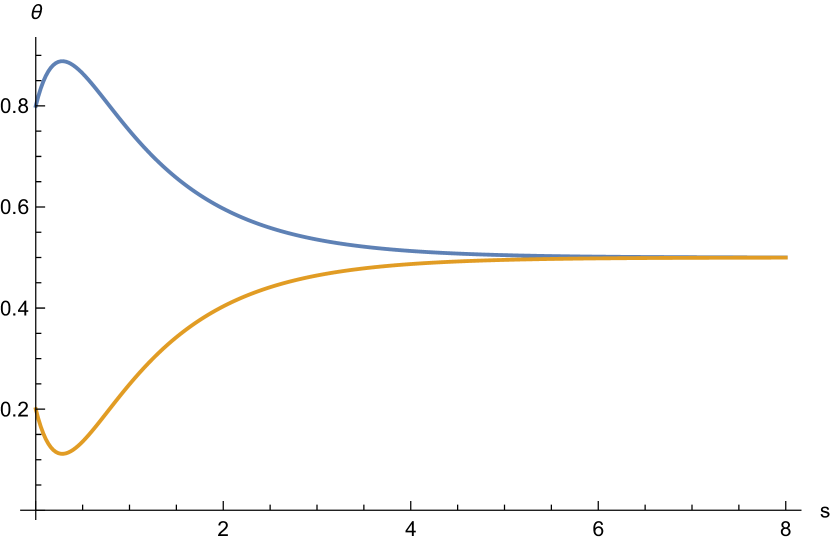
(a) Convergence of $\theta^{i}$.

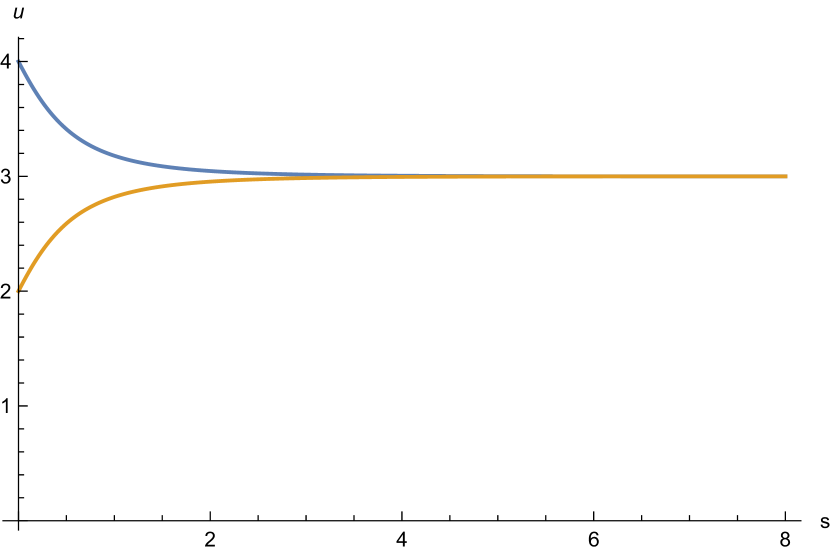
(b) Convergence of $u^{i}$.

Fig. 1. Evolution of $\theta$ and $u$ with the monotone flow, for $s\in[0,8]$.

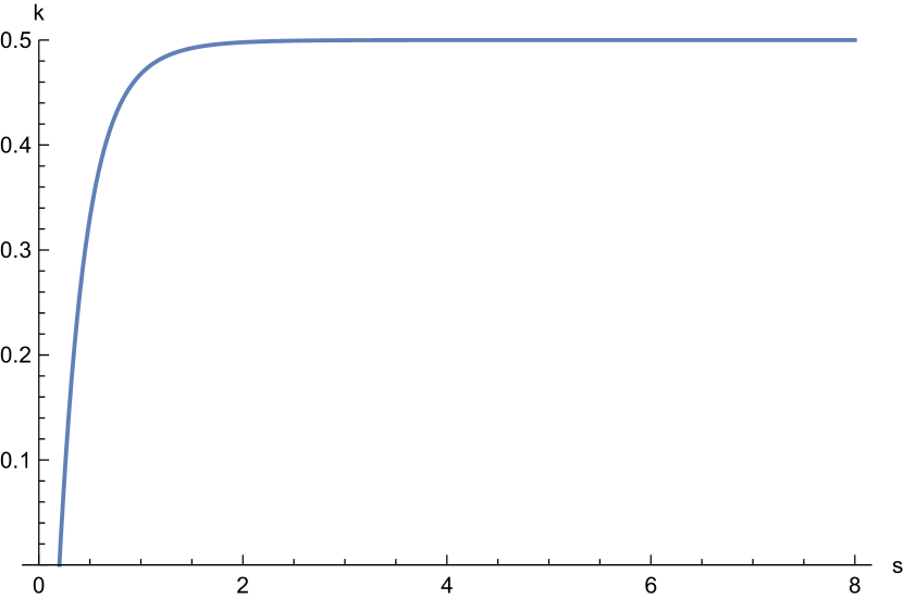
(a) Evolution of $k$.

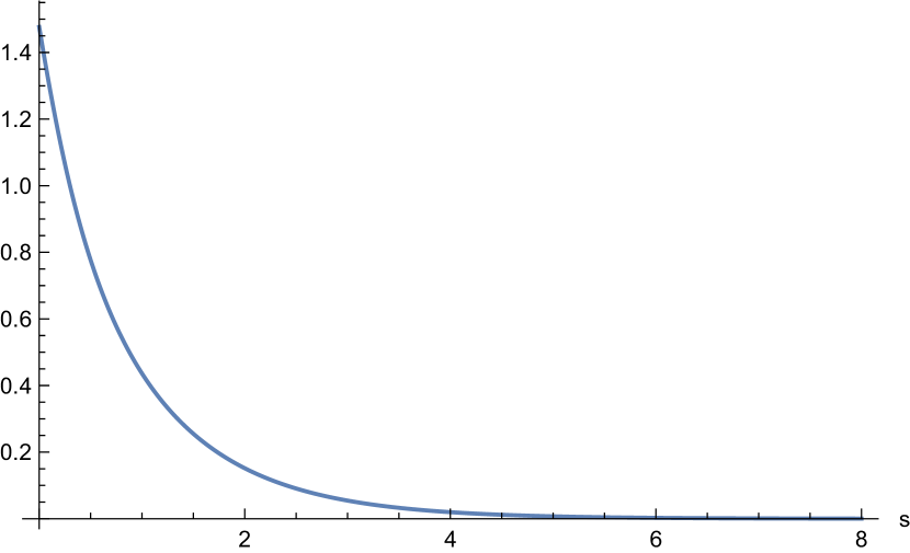
(b) Contraction of the norm.

Fig. 2. Evolution of $k$ and norm contraction, $\|(\theta,u)-(\bar{\theta},\bar{u})\|$.

Next, we consider the case where the iterates of $E_{\mu}$ do not preserve positivity. In Figure 3, we compare the evolution of $\theta$ by iterating $E_{\mu}$, without the projection, and using (20). In the first case, $\theta$ may not remain positive, although, in this example, convergence holds. In Figure 3, we plot the evolution through (20) of $\theta$ towards the analytical solution $\theta^{1}=\theta^{2}=0.5$.

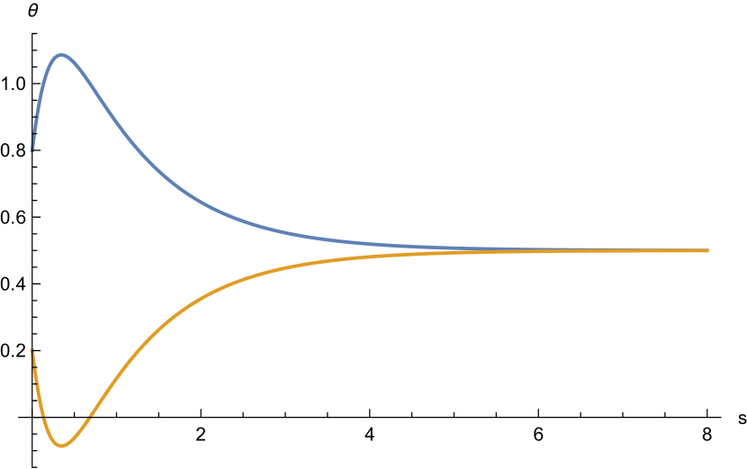
(a) Non positivity of the distribution using $E_{\mu}$.

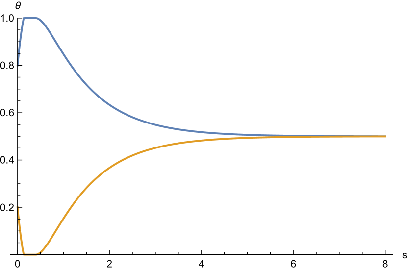
(b) Convergence using (20) while preserving the positivity of $\theta$.

Fig. 3. Comparison between the iterates of $E_{\mu}$ and $PE_{\mu}$ for $\theta^{1}_{0}=0.8$, $\theta^{2}_{0}=0.2$, $u^{1}_{0}=5$, and $u^{2}_{0}=2$.

As expected from its construction, $\theta$ is always non-negative and a probability. The contraction of the norm is similar to the previous case, see Figure 4(a).

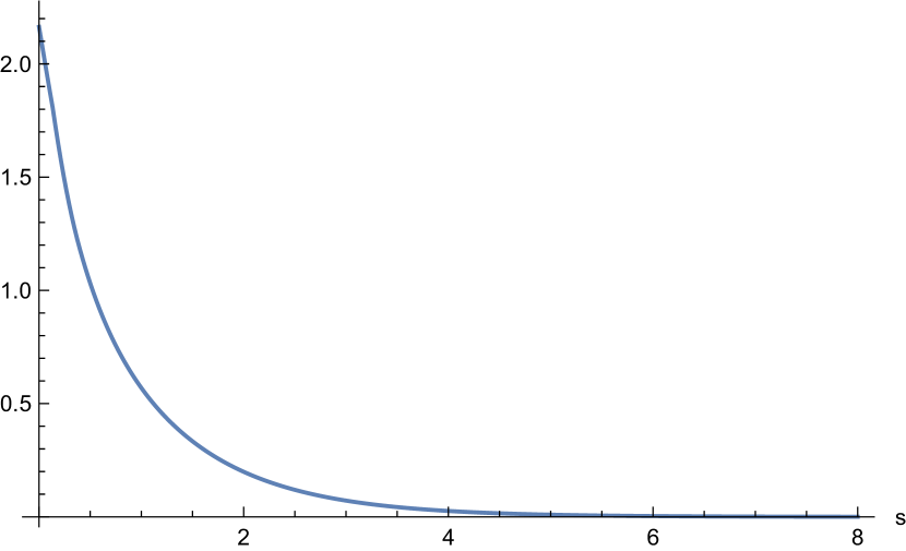
(a) Contraction of the norm.

Fig. 4. Evolution of the norm, $\|(\theta,u)-(\bar{\theta},\bar{u})\|$, using the projection method.

4. Initial-terminal value problems

The initial-terminal conditions in (3) are the key difficulty in the design of numerical methods for the time-dependent MFG, (2). Here, we extend the strategy from the previous section to handle initial-terminal conditions. We start with an arbitrary pair of functions, $(u(t,0),\theta(t,0))$, that satisfies (3) and build a family $(u(t,s),\theta(t,s))$, $s\geq 0$, that converges to a solution of (2)-(3) as $s\to\infty$, while preserving the boundary conditions for all $s\geq 0$.

4.1. Representation of functionals in $H^{1}$

We begin by discussing the representation of linear functionals in $H^{1}$. Consider the Hilbert space $H^{1}_{T}=\{\phi\in H^{1}([0,T],{\mathbb{R}}^{d}):\phi(T)=0\}$. For $\theta,u\in H^{1}([0,T],{\mathbb{R}}^{d})$, we consider the variational problem

(23) $$\min_{\phi\in H^{1}_{T}}\int_{0}^{T}\left[\frac{1}{2}(|\phi|^{2}+|\dot{\phi}|^{2})+\phi\cdot\left(\theta_{t}-\sum_{j}\theta^{j}\alpha^{*}(\Delta_{j}u,\theta,j)\right)\right]dt$$

A minimizer, $\phi\in H^{1}_{T}$, of the preceding functional represents the linear functional

$$\eta\mapsto-\int_{0}^{T}\eta\cdot\left(\theta_{t}-\sum_{j}\theta^{j}\alpha^{*}(\Delta_{j}u,\theta,j)\right)dt$$

for $\eta\in H^{1}_{T}$, as an inner product in $H^{1}_{T}$; that is,

$$\int_{0}^{T}\left(\eta\cdot\phi+\dot{\eta}\cdot\dot{\phi}\right)dt=-\int_{0}^{T}\eta\cdot\left(\theta_{t}-\sum_{j}\theta^{j}\alpha^{*}(\Delta_{j}u,\theta,j)\right)dt$$

for $\phi,\eta\in H^{1}_{T}$. The last identity is simply the weak form of the Euler-Lagrange equation for (23),

(24) $$-\ddot{\phi}+\phi=-\theta_{t}+\sum_{j}\theta^{j}\alpha^{*}(\Delta_{j}u,\theta,j),$$

whose boundary conditions are $\phi(T)=0$ and $\dot{\phi}(0)=0$. For $\theta,u\in H^{1}([0,T],{\mathbb{R}}^{d})$, we define

(25) $$\Phi(\theta,u,t)=\phi(t).$$

Next, let $H^{1}_{I}=\{\psi\in H^{1}([0,T],{\mathbb{R}}^{d}):\psi(0)=0\}$. For $\theta,u\in H^{1}([0,T],{\mathbb{R}}^{d})$, we consider the variational problem

(26) $$\min_{\psi\in H^{1}_{I}}\int_{0}^{T}\left[\frac{1}{2}(|\psi|^{2}+|\dot{\psi}|^{2})+\psi\cdot\left(u_{t}+h(\Delta_{i}u,\theta,i)\right)\right]dt.$$

The Euler-Lagrange equation for the preceding problem is

(27) $$-\ddot{\psi}+\psi=-u_{t}-h(\Delta_{i}u,\theta,i),$$

with the boundary conditions $\psi(0)=0$ and $\dot{\psi}(T)=0$. Moreover, if $\psi\in H^{1}_{I}$ minimizes the functional in (26), we have

$$\int_{0}^{T}\left(\eta\cdot\psi+\dot{\eta}\cdot\dot{\psi}\right)dt=\int_{0}^{T}\eta\cdot\left(-u_{t}-h(\Delta_{i}u,\theta,i)\right)dt$$

for $\eta,\psi\in H^{1}_{I}$. For $\theta,u\in H^{1}([0,T],{\mathbb{R}}^{d})$, we define

(28) $$\Psi(\theta,u,t)=\psi(t).$$

4.2. Monotone deformation flow

Next, we introduce the monotone deformation flow,

(29) $$\begin{cases}u_{s}^{i}(t,s)=\Phi^{i}(\theta(\cdot,s),u(\cdot,s),t)\\ \theta_{s}^{i}(t,s)=\Psi^{i}(\theta(\cdot,s),u(\cdot,s),t),\end{cases}$$

where $\Phi$ and $\Psi$ are given in (25) and (28). As we show in the next proposition, the previous flow is a contraction in $H^{1}$. Moreover, if $(\theta,u)$ solve (2)-(3), we have

$$\Phi(\theta,u,t)=\Psi(\theta,u,t)=0.$$

Hence, solutions of (2)-(3) are fixed points for (29).

Before stating the contraction property, we recall that the $H^{1}$-norm of a pair of functions is given by

$$\|(v,\eta)\|_{H^{1}}^{2}=\int_{0}^{T}\left(|v|^{2}+|\dot{v}|^{2}+|\eta|^{2}+|\dot{\eta}|^{2}\right)dt$$

for $v,\eta:[0,T]\to{\mathbb{R}}^{d}$.

Proposition 3.

Let $(u,\theta)$ and $(\tilde{u},\tilde{\theta})$ solve (29). Suppose $\theta,\tilde{\theta}\geq 0$. Then

$$\frac{d}{ds}\|(u,\theta)-(\tilde{u},\tilde{\theta})\|^{2}_{H^{1}}\leq 0,$$

with strict inequality if $(u,\theta)\neq(\tilde{u},\tilde{\theta})$.

Proof.

We have

$$\begin{split}\frac{1}{2}\frac{d}{ds}\int_{0}^{T}\left[(u-\tilde{u})^{2}+(u-\tilde{u})^{2}_{t}+(\theta-\tilde{\theta})^{2}+(\theta-\tilde{\theta})^{2}_{t}\right]dt\\ =\int_{0}^{T}\left[(u-\tilde{u})(u-\tilde{u})_{s}+(u-\tilde{u})_{t}(u-\tilde{u})_{ts}\right]dt\\ +\int_{0}^{T}\left[(\theta-\tilde{\theta})(\theta-\tilde{\theta})_{s}+(\theta-\tilde{\theta})_{t}(\theta-\tilde{\theta})_{ts}\right]dt.\end{split}$$

Using (29), the term in the right-hand side of previous equality becomes

$$\begin{split}\int_{0}^{T}\left[(u-\tilde{u})(\phi-\tilde{\phi})+(u-\tilde{u})_{t}(\phi-\tilde{\phi})_{t}\right]dt\\ +\int_{0}^{T}\left[(\theta-\tilde{\theta})(\psi-\tilde{\psi})+(\theta-\tilde{\theta})_{t}(\psi-\tilde{\psi})_{t}\right]dt\\ =\int_{0}^{T}(u-\tilde{u})(\phi-\tilde{\phi})dt+\left.\left[(u-\tilde{u})(\phi-\tilde{\phi})_{t}\right]\right|_{0}^{T}\\ -\int_{0}^{T}(u-\tilde{u})(\phi-\tilde{\phi})_{tt}dt\\ +\int_{0}^{T}(\theta-\tilde{\theta})(\psi-\tilde{\psi})dt+\left.\left[(\theta-\tilde{\theta})(\psi-\tilde{\psi})_{t}\right]\right|_{0}^{T}\\ -\int_{0}^{T}(\theta-\tilde{\theta})(\psi-\tilde{\psi})_{tt}dt,\end{split}$$

where we used integration by parts in the last equality. Because $u(T)=\tilde{u}(T)$, $\theta(0)=\tilde{\theta}(0)$, $\phi_{t}(0)=\tilde{\phi}_{t}(0)$, $\psi_{t}(T)=\tilde{\psi}_{t}(T)$, and using (24) and (27), we obtain

$$\frac{1}{2}\frac{d}{ds} \int_{0}^{T}(u-\tilde{u})^{2}+(u-\tilde{u})^{2}_{t}+(\theta-\tilde{\theta})^{2}+(\theta-\tilde{\theta})^{2}_{t}$$

$$=\int_{0}^{T}(u-\tilde{u})\left(\sum\theta^{j}\alpha^{*}(\Delta_{j}u,\theta,j)-\sum\tilde{\theta}\alpha^{*}(\Delta_{j}\tilde{u},\tilde{\theta},j)\right)$$

(30) $$-\int_{0}^{T}(\theta-\tilde{\theta})\left(h(\Delta_{i}u,\theta,i)-h(\Delta_{i}\tilde{u},\tilde{\theta},i)\right)$$

$$\leq\int_{0}^{T}-\gamma\|(\theta-\tilde{\theta})(t)\|^{2}-\sum_{i=1}^{d}\gamma_{i}(\theta^{i}+\tilde{\theta}^{i})(t)\|(\Delta_{i}u-\Delta_{i}\tilde{u})(t)\|^{2}dt,$$

due to Remark 1. ∎

4.3. Monotone discretization

To build our numerical method, we begin by discretizing (29). We look for a time-discretization of

$$A\left[\begin{array}[]{c}\theta\\ u\end{array}\right]=\left[\begin{array}[]{c}-\theta_{t}+f(u,\theta)\\ -u_{t}-h(u,\theta)\end{array}\right]$$

that preserves monotonicity, where $f(u,\theta)=\sum_{j}\tilde{\theta}^{j}\alpha^{*}(\Delta_{j}\tilde{u},\tilde{\theta},j)$.

For Hamilton-Jacobi equations, implicit schemes have good stability properties. Because the Hamilton-Jacobi equation in (29) is a terminal value problem, we discretize it using an explicit forward in time scheme (hence, implicit backward in time). Then, to keep the adjoint structure of $A$ at the discrete level, we are then required to choose an implicit discretization forward in time for the first component of $A$. Usually, implicit schemes have the disadvantage of requiring the numerical solution of non-linear equations at each time-step. Here, we discretize the operator $A$ globally, and we never need to solve implicit equations.

More concretely, we split $[0,T]$ into $N$ intervals of length $\delta t=\frac{T}{N}$. The vectors $\theta_{n}\in\mathcal{S}^{d}$ and $u_{n}\in{\mathbb{R}}^{d}$, $0\leq n\leq N$ approximate $\theta$ and $u$ at time $\frac{nT}{N}$. We set $\mathcal{M}_{N}=(\mathcal{S}^{d}\times{\mathbb{R}}^{d})^{N+1}$ and define

(31) $$A^{N}\left[\begin{array}[]{c}\theta\\ u\end{array}\right]_{n}=\left[\begin{array}[]{c}-\frac{\theta_{n+1}^{i}-\theta_{n}^{i}}{\delta t}+f(u_{n+1}^{i},\theta_{n+1}^{i})+k_{n}\\ -\frac{u_{n+1}^{i}-u_{n}^{i}}{\delta t}-h(u_{n}^{i},\theta_{n}^{i})\end{array}\right],$$

where

$$k_{n}(s)=-\frac{1}{d}\sum_{i=1}^{d}\left(-\frac{\delta\theta^{i}_{n}}{\delta t}+f(u_{n+1}^{i},\theta_{n+1}^{i})\right)$$

and $\delta\theta^{i}_{n}=\theta_{n+1}^{i}-\theta_{n}^{i}$. Next, we show that $A^{N}$ is a monotone operator in the convex subset of vectors in $\mathcal{M}$ that satisfy the initial-terminal conditions in (3).

Proposition 4.

$A^{N}$ is monotone in the convex subset $\mathcal{M}_{N}$ of all $(\theta,u)\in(\mathcal{S}^{d}\times{\mathbb{R}}^{d})^{N+1}$ such that $\theta_{0}=\bar{\theta}_{0}$ and $u_{N}=\bar{u}_{T}$. Moreover, we have the inequality

$$\left\langle A^{N}\left[\begin{array}[]{c}\theta\\ u\end{array}\right]-A^{N}\left[\begin{array}[]{c}\tilde{\theta}\\ \tilde{u}\end{array}\right],\left[\begin{array}[]{c}\theta\\ u\end{array}\right]-\left[\begin{array}[]{c}\tilde{\theta}\\ \tilde{u}\end{array}\right]\right\rangle$$

$$\leq\sum_{n=1}^{N-1}\left(-\gamma\|(\theta-\tilde{\theta})(t)\|^{2}-\sum_{i=1}^{d}\gamma_{i}(\theta^{i}+\tilde{\theta}^{i})(t)\|(\Delta_{i}u-\Delta_{i}\tilde{u})(t)\|^{2}\right).$$

Proof.

We begin by computing

$$\left\langle A^{N}\left[\begin{array}[]{c}\theta\\ u\end{array}\right]-A^{N}\left[\begin{array}[]{c}\tilde{\theta}\\ \tilde{u}\end{array}\right],\left[\begin{array}[]{c}\theta\\ u\end{array}\right]-\left[\begin{array}[]{c}\tilde{\theta}\\ \tilde{u}\end{array}\right]\right\rangle$$

$$=\sum_{n=0}^{N-1}(\theta_{n}-\tilde{\theta}_{n})\left(-\frac{u_{n+1}-u_{n}}{\delta t}-h(u_{n},\theta_{n})+\frac{\tilde{u}_{n+1}-\tilde{u}_{n}}{\delta t}+h(\tilde{u}_{n},\tilde{\theta}_{n})\right)$$

$$+(u_{n+1}-\tilde{u}_{n+1})\Big{(}-\frac{\theta_{n+1}-\theta_{n}}{\delta t}+f(u_{n+1},\theta_{n+1})+k_{n}$$

$$+\frac{\tilde{\theta}_{n+1}-\tilde{\theta}_{n}}{\delta t}-f(\tilde{u}_{n+1},\tilde{\theta}_{n+1})-\tilde{k}_{n}\Big{)}.$$

Developing the sums and relabeling the indices, the preceding expression becomes

$$\sum_{n=1}^{N-1}(\theta_{n}-\tilde{\theta}_{n})\left(-\frac{u_{n+1}-u_{n}}{\delta t}-h(u_{n},\theta_{n})+\frac{\tilde{u}_{n+1}-\tilde{u}_{n}}{\delta t}+h(\tilde{u}_{n},\tilde{\theta}_{n})\right)$$

$$+(\theta_{0}-\tilde{\theta}_{0})\left(-\frac{u_{1}-u_{0}}{\delta t}-h(u_{0},\theta_{0})+\frac{\tilde{u}_{1}-\tilde{u}_{0}}{\delta t}+h(\tilde{u}_{0},\theta_{0})\right)$$

$$+\sum_{n=1}^{N-1}(u_{n}-\tilde{u}_{n})\left(-\frac{\theta_{n}-\theta_{n-1}}{\delta t}+f(u_{n},\theta_{n})+\frac{\tilde{\theta}_{n}-\tilde{\theta}_{n-1}}{\delta t}-f(\tilde{u}_{n},\tilde{\theta}_{n})\right)$$

$$+(u_{N}-\tilde{u}_{N})\left(-\frac{\theta_{N}-\theta_{N-1}}{\delta t}+f(u_{N},\theta_{N})+\frac{\tilde{\theta}_{N}-\tilde{\theta}_{N-1}}{\delta t}-f(\tilde{u}_{N},\tilde{\theta}_{N})\right).$$

The second and last lines above are zero since $\theta_{0}=\tilde{\theta}_{0}=\bar{\theta}_{0}$ and $u_{N}=\tilde{u}_{N}=\bar{u}_{T}$. Using Remark 1, we obtain

$$\left\langle A\left[\begin{array}[]{c}\theta\\ u\end{array}\right]-A\left[\begin{array}[]{c}\tilde{\theta}\\ \tilde{u}\end{array}\right],\left[\begin{array}[]{c}\theta\\ u\end{array}\right]-\left[\begin{array}[]{c}\tilde{\theta}\\ \tilde{u}\end{array}\right]\right\rangle$$

$$\leq\sum_{n=1}^{N-1}\left(-\gamma\|(\theta-\tilde{\theta})(t)\|^{2}-\sum_{i=1}^{d}\gamma_{i}(\theta^{i}+\tilde{\theta}^{i})(t)\|(\Delta_{i}u-\Delta_{i}\tilde{u})(t)\|^{2}\right)$$

$$-\sum_{n=1}^{N-1}(\theta_{n}-\tilde{\theta}_{n})\left(\frac{u_{n+1}-\tilde{u}_{n+1}}{\delta t}-\frac{u_{n}-\tilde{u}_{n}}{\delta t}\right)$$

$$-\sum_{n=1}^{N-1}(u_{n}-\tilde{u}_{n})\left(\frac{\theta_{n}-\tilde{\theta}_{n}}{\delta t}-\frac{\theta_{n-1}-\tilde{\theta}_{n-1}}{\delta t}\right).$$

We now show that the last two lines add to zero. Let $a_{n}=\theta_{n}-\tilde{\theta}_{n}$ and $b_{n}=u_{n}-\tilde{u}_{n}$. Accordingly, we have

$$-\frac{1}{\delta t}\sum_{n=1}^{N-1}a_{n}(b_{n+1}-b_{n})-\frac{1}{\delta t}\sum_{n=1}^{N-1}b_{n}(a_{n}-a_{n-1})$$

$$=\frac{1}{\delta t}\sum_{n=1}^{N-1}b_{n+1}(a_{n+1}-a_{n})-(b_{N}a_{N}-b_{1}a_{1})-\frac{1}{\delta t}\sum_{n=0}^{N-2}b_{n+1}(a_{n+1}-a_{n})$$

$$=\frac{1}{\delta t}(b_{1}a_{0}-b_{N}a_{N-1})=0,$$

where we summed by parts the first member and relabeled the index $n$ in the last member of the first line. The last equality follows from the assumption in the statement, $a_{0}=\theta_{0}-\tilde{\theta}_{0}=0$ and $b_{N}=u_{N}-\tilde{u}_{N}=0$. ∎

Using the techniques in [6], we prove the convergence of the solutions of the discretized problem as $\delta t\to 0$. As usual, we discretize the time interval, $[0,T]$, into $N+1$ equispaced points.

Proposition 5.

Let $(\theta^{N},u^{N})\in{\mathcal{M}}_{N}$, be a solution of

$$A^{N}\left[\begin{array}[]{c}\theta^{N}\\ u^{N}\end{array}\right]_{n}=\left[\begin{array}[]{c}0\\ 0\end{array}\right]$$

satisfying the initial-terminal conditions in (3). Suppose $u^{N}$ is uniformly bounded. Consider the step functions, $\bar{u}^{N}$, $\bar{\theta}^{N}$, taking the values $\bar{u}^{Ni}_{n}\in{\mathbb{R}}$ and $\bar{\theta}_{n}^{Ni}\in\mathcal{S}$ in $[\frac{(n-1)T}{N},\frac{nT}{N}]$, with $0\leq n\leq N$, for $i\in I_{d}$, respectively. Then, extracting a subsequence if necessary, $\bar{u}^{Ni}\rightharpoonup\bar{u}^{i}$ and $\bar{\theta}^{Ni}\rightharpoonup\theta^{i}$, weakly-* in $L^{\infty}$ for $i\in I_{d}$. Furthermore, $(\bar{u},\bar{\theta})$ is a weak solution of (2).

Proof.

Because $u^{N}$ is bounded by hypothesis and $\theta^{N}$ is bounded since it is a probability measure, the weak-* convergence in $L^{\infty}$ is immediate. Hence, there exist $\bar{u}^{i}\in L^{\infty}([0,T])$ and $\theta^{i}\in L^{\infty}([0,T])$ as claimed.

Let $\tilde{u}^{i},\tilde{\theta}^{i}\in C^{\infty}([0,T])$, with $\tilde{\theta}^{i}\geq 0$ for all $i\in I_{d}$, and $\sum_{i\in I_{d}}\tilde{\theta}^{i}=1$. Suppose further that $\tilde{u}^{i},\tilde{\theta}^{i}$ satisfy the boundary conditions in (3). Let $\tilde{u}_{n}^{N}=\tilde{u}\left(\frac{n}{N}T\right)$, $\tilde{\theta}_{n}^{N}=\tilde{\theta}\left(\frac{n}{N}T\right)$ be the vectors whose components are $\tilde{u}_{n}^{Ni}$ and $\tilde{\theta}_{n}^{Ni}$, respectively. By the monotonicity of $A^{N}$, we have

$$0 \leq\left\langle A^{N}\left[\begin{array}[]{c}\tilde{\theta}^{N}\\ \tilde{u}^{N}\end{array}\right],\left[\begin{array}[]{c}\tilde{\theta}^{N}\\ \tilde{u}^{N}\end{array}\right]-\left[\begin{array}[]{c}\theta^{N}\\ u^{N}\end{array}\right]\right\rangle$$

$$=O\left(\frac{1}{N}\right)+\left\langle A^{N}\left[\begin{array}[]{c}\tilde{\theta}\\ \tilde{u}\end{array}\right],\left[\begin{array}[]{c}\tilde{\theta}\\ \tilde{u}\end{array}\right]-\left[\begin{array}[]{c}\bar{\theta}^{N}\\ \bar{u}^{N}\end{array}\right]\right\rangle,$$

taking the limit $N\to\infty$ gives the result. ∎

4.4. Monotone discretization for the $H^{1}$ projections

Next, we discuss the representation of linear functionals for the discrete problem. For that, proceeding as in Section 4.1, we compute the optimality conditions of the discretized versions of (23) and (26).

Fix $(u,\theta)\in\mathcal{M}_{N}$ and consider the following discrete analog to (23):

$$\min_{\phi\in\tilde{H}^{1}_{T}}\delta t\sum_{n=1}^{N}\frac{1}{2}\left(\phi_{n}^{2}+\left(\frac{\delta\phi_{n-1}}{\delta t}\right)^{2}\right)+\phi_{n}\left(\frac{\delta\theta_{n-1}}{\delta t}-f(u_{n},\theta_{n})\right),$$

where $\delta g_{n}=g_{n+1}-g_{n}$, and $\tilde{H}^{1}_{T}=\{\phi=(\phi_{0},\ldots,\phi_{N})\in({\mathbb{R}}^{d})^{(N+1)}:\phi_{N}=0\}$. The corresponding optimality conditions (the discrete Euler-Lagrange equation) is

(32) $$-\frac{\delta(\delta\phi_{n-1})}{(\delta t)^{2}}+\phi_{n}=-\frac{\delta\theta_{n-1}}{\delta t}+f(u_{n},\theta_{n}),$$

for $n=1,\ldots,N-1$, coupled with the boundary conditions $\phi_{N}=0$ and $\phi_{1}=\phi_{0}$.

A minimizer of the problem above represents the following discrete linear functional

$$\eta\mapsto-\sum_{n=1}^{N}\eta_{n}\cdot\left(\frac{\delta\phi_{n-1}}{\delta t}-f(u_{n},\theta_{n})\right)\delta t$$

as an inner product in $\tilde{H}^{1}_{T}$

$$\sum_{n=1}^{N}\left(\eta_{n}\cdot\phi_{n}\delta t+\frac{1}{\delta t}\delta\eta_{n-1}\cdot\delta\phi_{n-1}\right)=-\sum_{n=1}^{N}\eta_{n}\cdot\left(\frac{\delta\phi_{n-1}}{\delta t}-f(u_{n},\theta_{n})\right)\delta t.$$

For $(\theta_{n},u_{n})\in\mathcal{M}_{N}$, we define

(33) $$\Phi(\theta_{n},u_{n})=\phi_{n}.$$

We now examine a second discrete variational problem corresponding to (26). For $(u,\theta)\in\mathcal{M}_{N}$, consider

$$\min_{\psi\in\tilde{H}^{1}_{I}}\delta t\sum_{n=0}^{N-1}\frac{1}{2}\left(\psi_{n}^{2}+\left(\frac{\delta\psi_{n}}{\delta t}\right)^{2}\right)+\psi_{n}\left(\frac{\delta u_{n}}{\delta t}+h(u_{n},\theta_{n})\right),$$

where $\tilde{H}^{1}_{I}=\{\psi=(\psi_{0},\ldots,\psi_{N})\in({\mathbb{R}}^{d})^{(N+1)}:\psi_{0}=0\}$.

The discrete Euler-Lagrange equation is

(34) $$-\frac{\delta(\delta\psi_{n-1})}{(\delta t)^{2}}+\psi_{n}=-\frac{\delta u_{n}}{\delta t}-h(u_{n},\theta_{n})$$

for $n=1,\ldots,N-1$, together with the conditions $\psi_{0}=0$ and $\psi_{N}=\psi_{N-1}$.

From the Euler-Lagrange equation, we obtain the following representation formula in the Hilbert space $\{\psi\in H_{n}^{1}(\{0,\ldots,N\}):\psi_{0}=0\}$:

$$\sum_{n=0}^{N-1}\left(\eta\cdot\psi+\delta\eta\cdot\delta\psi\right)\delta t=\sum_{0}^{N}\eta\cdot\left(-\frac{\delta u_{n}}{\delta t}-h(u_{n},\theta_{n})\right)\delta t.$$

Finally, we define

(35) $$\Psi(\theta_{n},u_{n})=\psi_{n},$$

for $(u,\theta)\in\mathcal{M}_{N}$.

Proposition 6.

Let $\Phi$ and $\Psi$ be given by (33) and (35). Consider the following operator:

(36) $$Q_{A}\left[\begin{array}[]{c}\theta\\ u\end{array}\right]=\left[\begin{array}[]{c}\Phi\\ \Psi\end{array}\right].$$

Let ${\mathcal{M}}_{N}^{\bar{\theta}_{0},\bar{u}_{T}}$ be the set of all $(\theta,u)\in{\mathcal{M}}_{N}$ that satisfy the initial condition $\theta_{0}=\bar{\theta}_{0}$ and the terminal condition $u_{N}=\bar{u}_{T}$. Then, $Q_{A}$ is monotone with respect to the discrete $H^{1}_{N}$ inner product corresponding to the norm

(37) $$\|(\eta,\nu)\|_{H^{1}_{N}}^{2}=\sum_{n=0}^{N-1}|\eta_{n}|^{2}+|\delta\eta_{n}|^{2}+|\nu_{n}|^{2}+|\delta\nu_{n}|^{2}.$$

Proof.

Let $(u,\theta)\in{\mathcal{M}}_{N}^{\bar{\theta}_{0},\bar{u}_{T}}$ and $(\tilde{u},\tilde{\theta})\in{\mathcal{M}}_{N}^{\bar{\theta}_{0},\bar{u}_{T}}$. Let $\phi,\tilde{\phi}$ and $\psi,\tilde{\psi}$ be given by (33) and (35). We begin computing

(46) $$\left\langle Q_{A}\left[\begin{array}[]{c}\theta\\ u\end{array}\right]-Q_{A}\left[\begin{array}[]{c}\tilde{\theta}\\ \tilde{u}\end{array}\right],\left[\begin{array}[]{c}\theta\\ u\end{array}\right]-\left[\begin{array}[]{c}\tilde{\theta}\\ \tilde{u}\end{array}\right]\right\rangle_{H^{1}_{N}}$$

$$=\sum_{n=0}^{N-1}(\theta_{n}-\tilde{\theta}_{n})(\psi_{n}-\tilde{\psi}_{n})+\frac{\delta(\theta_{n}-{\tilde{\theta}}_{n})}{\delta t}\frac{\delta(\psi_{n}-\tilde{\psi}_{n})}{\delta t}$$

$$\quad+(u_{n}-\tilde{u}_{n})(\phi_{n}-\tilde{\phi}_{n})+\frac{\delta(u_{n}-{\tilde{u}}_{n})}{\delta t}\frac{\delta({\phi}_{n}-{\tilde{\phi}}_{n})}{\delta t}$$

$$=\sum_{n=0}^{N-1}(\theta_{n}-\tilde{\theta}_{n})(\psi_{n}-\tilde{\psi}_{n})+(u_{n}-\tilde{u}_{n})(\phi_{n}-\tilde{\phi}_{n})$$

$$\quad+\frac{1}{\delta t}\sum_{n=0}^{N-1}\left(\frac{\theta_{n+1}-\theta_{n}}{\delta t}-\frac{\tilde{\theta}_{n+1}-\tilde{\theta}_{n}}{\delta t}\right)(\delta{\psi}_{n}-\delta{\tilde{\psi}}_{n})$$

(47) $$\quad+\frac{1}{\delta t}\sum_{n=0}^{N-1}\left(\frac{u_{n+1}-u_{n}}{\delta t}-\frac{\tilde{u}_{n+1}-\tilde{u}_{n}}{\delta t}\right)(\delta{\phi}_{n}-\delta{\tilde{\phi}}_{n}).$$

Reorganizing, we see that the previous two lines are equal to

$$\frac{1}{(\delta t)^{2}}\sum_{n=0}^{N-1}\left[(\theta_{n+1}-\tilde{\theta}_{n+1})-(\theta_{n}-\tilde{\theta}_{n})\right](\delta{\psi}_{n}-\delta\tilde{\psi}_{n})$$

(48) $$\quad+\left[(u_{n+1}-\tilde{u}_{n+1})-(u_{n}-\tilde{u}_{n})\right](\delta{\phi}_{n}-\delta{\tilde{\phi}}_{n}).$$

Using the notation

$$a_{n}=\theta_{n}-\tilde{\theta}_{n},\quad b_{n}=\delta{\psi}_{n}-\delta{\tilde{\psi}}_{n},\quad c_{n}=u_{n}-\tilde{u}_{n},\text{ and }d_{n}=\delta{\phi}_{n}-\delta{\tilde{\phi}}_{n},$$

we write (4.4) multiplied by $(\delta t)^{2}$ as

$$\sum_{n=0}^{N-1}b_{n}\delta a_{n}+d_{n}\delta c_{n} =b_{N-1}\delta a_{N-1}+d_{N-1}\delta c_{N-1}+\sum_{n=0}^{N-2}b_{n}\delta a_{n}+d_{n}\delta c_{n}$$

$$=b_{N-1}\delta a_{N-1}+d_{N-1}\delta c_{N-1}$$

$$+a_{N-1}b_{N-1}-a_{0}b_{0}-\sum_{n=0}^{N-2}a_{n+1}\delta b_{n}$$

(49) $$+c_{N-1}d_{N-1}-c_{0}d_{0}-\sum_{n=0}^{N-2}c_{n+1}\delta d_{n},$$

where we used summation by parts in the last equality. Because $\psi_{N}=\psi_{N-1}$, we have that $b_{N-1}=0$. Moreover, since $\theta_{0}=\tilde{\theta}_{0}$, we have $a_{0}=0$, and $\phi_{1}=\phi_{0}$ implies $d_{0}=0$. Thus, we further have

$$d_{N-1}\delta c_{N-1} =d_{N-1}\left(u_{N}-\tilde{u}_{N}-(u_{N-1}-\tilde{u}_{N-1})\right)$$

$$=-d_{N-1}(u_{N-1}-\tilde{u}_{N-1})$$

$$=-c_{N-1}d_{N-1},$$

where we used the terminal condition $u_{N}=\tilde{u}_{N}$. According to these identities, (4.4) becomes

$$\sum_{n=0}^{N-1}b_{n}\delta a_{n}+d_{n}\delta c_{n} =-\sum_{n=0}^{N-2}a_{n+1}\delta b_{n}+c_{n+1}\delta d_{n}.$$

Therefore, (4.4) can be written as

(50) $$-\sum_{n=0}^{N-2}\frac{\theta_{n+1}-\tilde{\theta}_{n+1}}{(\delta t)^{2}}\left(\delta^{2}\psi_{n}-\delta^{2}\tilde{\psi}_{n}\right)-\sum_{n=0}^{N-2}\frac{u_{n+1}-\tilde{u}_{n+1}}{(\delta t)^{2}}\left(\delta^{2}\phi_{n}-\delta^{2}\tilde{\phi}_{n}\right).$$

Shifting the index $n+1$ into $n$ in (50), we obtain

$$-\sum_{n=1}^{N-1}\frac{\theta_{n}-\tilde{\theta}_{n}}{(\delta t)^{2}}\left(\delta^{2}\psi_{n-1}-\delta^{2}\tilde{\psi}_{n-1}\right)-\sum_{n=1}^{N-1}\frac{u_{n}-\tilde{u}_{n}}{(\delta t)^{2}}\left(\delta^{2}\phi_{n-1}-\delta^{2}\tilde{\phi}_{n-1}\right).$$

Using the Euler-Lagrange equations (32) and (34) in the preceding expression, yields

$$-\sum_{n=1}^{N-1}(\theta_{n}-\tilde{\theta}_{n})\left(\psi_{n}+\frac{u_{n+1}-u_{n}}{\delta t}+h(u_{n},\theta_{n})-\tilde{\psi}_{n}-\frac{\tilde{u}_{n+1}-\tilde{u}_{n}}{\delta t}-h(\tilde{u}_{n},\tilde{\theta}_{n})\right)$$

$$-\sum_{n=1}^{N-1}(u_{n}-\tilde{u}_{n})\left(\phi_{n}+\frac{\theta_{n}-\theta_{n-1}}{\delta t}-f(u_{n},\theta_{n})-\tilde{\phi}_{n}-\frac{\tilde{\theta}_{n}-\tilde{\theta}_{n-1}}{\delta t}+f(\tilde{u}_{n},\tilde{\theta}_{n})\right).$$

Finally, plugging the previous result into (46), we obtain

$$-\sum_{N=1}^{N-1}(\theta_{n}-\tilde{\theta}_{n})\left(\frac{u_{n+1}-\tilde{u}_{n+1}}{\delta t}-\frac{u_{n}-\tilde{u}_{n}}{\delta t}+h(u_{n},\theta_{n})-h(\tilde{u}_{n},\tilde{\theta}_{n})\right)$$

$$-\sum_{n=1}^{N-1}(u_{n}-\tilde{u}_{n})\left(\frac{\theta_{n}-\tilde{\theta}_{n}}{\delta t}-\frac{\theta_{n-1}-\tilde{\theta}_{n-1}}{\delta t}-f(u_{n},\theta_{n})+f(\tilde{u}_{n},\tilde{\theta}_{n})\right)$$

$$\leq-\gamma\|(\theta-\tilde{\theta})(s)\|^{2}-\sum_{i=1}^{d}\gamma_{i}(\theta^{i}+\tilde{\theta}^{i})(s)\|(\Delta_{i}u-\Delta_{i}\tilde{u})(s)\|^{2},$$

using Remark 1 and arguing as at the end of Subsection 4.3. ∎

4.5. Projection algorithm

As shown in Section 3, the monotone flow may not keep $\theta$ positive. Thus, to preserve probabilities and prevent $\theta$ to take negative values, we define a projection operator through the following optimization problem. Given $(\eta,w)\in{\mathcal{M}}_{N}$, we solve

(51) $$\begin{cases}\min_{\lambda^{i}_{n}}\sum_{i=1}^{d}(\eta^{i}_{n}-\lambda^{i}_{n})^{2}\\ \sum_{i=1}^{d}\lambda^{i}_{n}=1,\quad\lambda^{i}_{n}\geq 0\end{cases}$$

for $n\in\{0,\ldots,N\}$. Then, we set

$$P\left[\begin{array}[]{c}\eta\\ w\end{array}\right]_{n}=\left[\begin{array}[]{c}\lambda_{n}\\ w_{n}\end{array}\right]$$

for $0\leq n\leq N$. We note that if $\eta_{n}$ is a probability, then $\lambda_{n}=\eta_{n}$. Moreover, $P$ is a contraction.

Now, we introduce the following iterative scheme:

(52) $$w_{k+1}=P\left[w_{k}-\upsilon Q_{A}[w_{k}]\right],$$

where $w_{k}=(\theta_{k},u_{k})$, $Q_{A}$ is defined in (36), and $\upsilon>0$ is the step size.

Proposition 7.

For $\upsilon$ small enough, the map (52) is a contraction.

Proof.

The operator $E_{\upsilon}$ is a contraction, because $Q_{A}$ is a monotone Lipschitz map, see Proposition 6. ∎

Proposition 8.

Let $(\bar{\theta},\bar{u})\in{\mathcal{M}}_{N}$ solve

$$A^{N}\left[\begin{array}[]{c}\theta\\ u\end{array}\right]=\left[\begin{array}[]{c}0\\ 0\end{array}\right],$$

with $u_{N}=\bar{u}_{T}$ and $\theta_{0}=\bar{\theta}_{0}$. Then, $(\bar{\theta},\bar{u})$ is a fixed point of (52).

Conversely, let $(\tilde{\theta},\tilde{u})\in{\mathcal{M}}_{N}$ be a fixed point of (52) with $\tilde{\theta}>0$. Then, there exists a weak solution to (2), $(\bar{\theta},\bar{u})$ with $\bar{\theta}=\tilde{\theta}$ and $\bar{u}$ given by

(53) $$\frac{\delta\bar{u}^{i}_{n}}{\delta t}=-h(\Delta_{i}\tilde{u},\theta,i),$$

with $\bar{u}_{N}=\bar{u}_{T}$.

Proof.

The first claim of the proposition is immediate from the definition of $Q_{A}$. To prove the second part, let $(\tilde{\theta},\tilde{u})\in{\mathcal{M}}_{N}$ be a fixed point of (52). For all $n\in\{0,\ldots,N\}$ and $i\in I_{d}$, we have

$$\tilde{u}^{i}_{n}=\tilde{u}^{i}_{n}+\upsilon\phi_{n}(\tilde{u}_{n},\tilde{\theta}_{n}).$$

Therefore, $\phi_{n}(\tilde{u}_{n},\tilde{\theta}_{n})=0$. Hence, from the uniqueness of the solution of (32), we conclude that

$$-\frac{\delta\tilde{\theta}_{n-1}}{\delta t}+f(\tilde{u}_{n},\tilde{\theta}_{n})=0$$

Furthermore, for $\tilde{\theta}_{n}^{i}=\lambda_{n}^{i}$, where $\lambda_{n}^{i}$ solves (51), we have

$$\begin{split}\tilde{\theta}_{n}^{i}&=P\left[\tilde{\theta}_{n}^{i}-\upsilon\psi_{n}(\tilde{u}_{n},\tilde{\theta}_{n})\right]\\ &=\left(\tilde{\theta}_{n}^{i}-\upsilon\psi_{n}(\tilde{u}_{n},\tilde{\theta}_{n})+\upsilon\kappa_{n}\right)^{+}\end{split}$$

For some $\kappa_{n}\geq 0$. If $\tilde{\theta}^{i}_{n}>0$, $\psi_{n}(\tilde{u}_{n},\tilde{\theta}_{n})=\kappa_{n}$. Otherwise, $\psi_{n}(\tilde{u}_{n},\tilde{\theta}_{n})\geq\kappa_{n}$.

If $\tilde{\theta}^{i}_{n}>0$, using the fact that $\psi$ solves (34), we gather

$$\frac{\delta\tilde{u}^{i}_{n}}{\delta t}-\frac{1}{d-1}\sum_{j\neq i}\frac{\delta\tilde{u}^{j}_{n}}{\delta t}=\frac{1}{d-1}\sum_{j\neq i}h(\Delta_{j}\tilde{u}_{n},\theta,j)-h(\Delta_{i}\tilde{u}_{n},\theta,i).$$

Now, we define $\bar{u}$ as in the statement of the proposition. A simple computation gives

$$\frac{\delta\bar{u}^{i}_{n}}{\delta t}-\frac{\delta\bar{u}^{j}_{n}}{\delta t}=\frac{\delta\tilde{u}^{i}_{n}}{\delta t}-\frac{\delta\tilde{u}^{j}_{n}}{\delta t}.$$

Hence, $\Delta_{j}\bar{u}_{n}=\Delta_{j}\tilde{u}_{n}$. Consequently,

$$\frac{\delta\bar{u}^{i}_{n}}{\delta t}=-h(\Delta_{i}\bar{u},\theta,i).$$

Thus, $(\bar{\theta},\bar{u})$ solves (2). ∎

4.6. Numerical examples

Finally, we present numerical simulations for the time-dependent paradigm-shift problem. As explained before, we discretize the time variable, $t\in[0,T]$, into $N$ intervals of length $\delta t=\frac{T}{N}$. We then have $N$ equations for each state. Because $d=2$, this system consists of $4N$ equations evolving according to (52).

To compute approximate solutions to (16)-(17), we use the projection algorithm, (52), with $N=450$. We first consider a case where the analytical solution can be computed explicitly. We choose $\theta^{1}=\theta^{2}=\frac{1}{2}$. Thus, from (16), it follows that $u^{1}=u^{2}$ are affine functions of $t$ with $u^{1}_{t}=u^{2}_{t}-\frac{1}{2}$. Our results are depicted in Figures 5, 6, and 7. In Figure 5, for $t\in[0,T]$, $T=8$, we plot the initial guess ($s=0$) for $\theta$ and $u$, and the analytical solution. In Figure 6, we see the evolution of density of players and the value functions for $s\in[0,20]$. The final results, $s=100$, are shown in Figure 7. Finally, in Figure 8, we show the evolution of the $H^{1}$ norm of the difference between the analytical, $(\tilde{u},\tilde{\theta})$, and computed solution, $(u,\theta)$. The norm $\|(\tilde{u},\tilde{\theta})-(u,\theta)\|_{H^{1}([0,T])}^{2}(s)$ is computed as

$$\sum_{j=0}^{N-1}\sum_{i=1}^{2}\delta t\left(|\tilde{u}^{i}_{j}-u^{i}_{j}|^{2}+|\dot{\tilde{u}}^{i}_{j}-\dot{u}^{i}_{j}|^{2}+|\tilde{\theta}^{i}_{j}-\theta^{i}_{j}|^{2}+|\dot{\tilde{\theta}}^{i}_{j}-\dot{\theta}^{i}_{j}|^{2}\right)(s)$$

for $s\geq 0$, where $v^{i}_{j}=v^{i}(t_{j},s)$ and $\delta t$ is size of the time-discretization step.

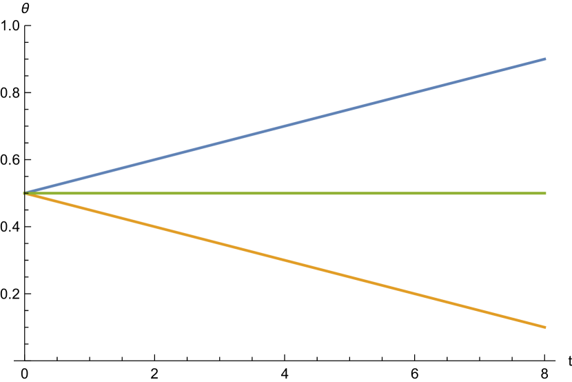
(a) Initial condition $\theta(\cdot,s=0)$ vs exact solution.

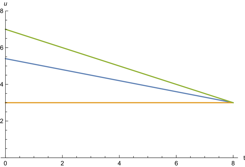
(b) Initial condition $u(\cdot,s=0)$.

Fig. 5. The blue lines correspond to the initial values ($s=0$) for state 1, $(\theta^{1},u^{1})$, the orange lines to the initial values for state 2, $(\theta^{2},u^{2})$. The green lines represent the analytical solution $\theta^{1}=\theta^{2}$ and $u^{1}=u^{2}$ for $t\in[0,T]$.

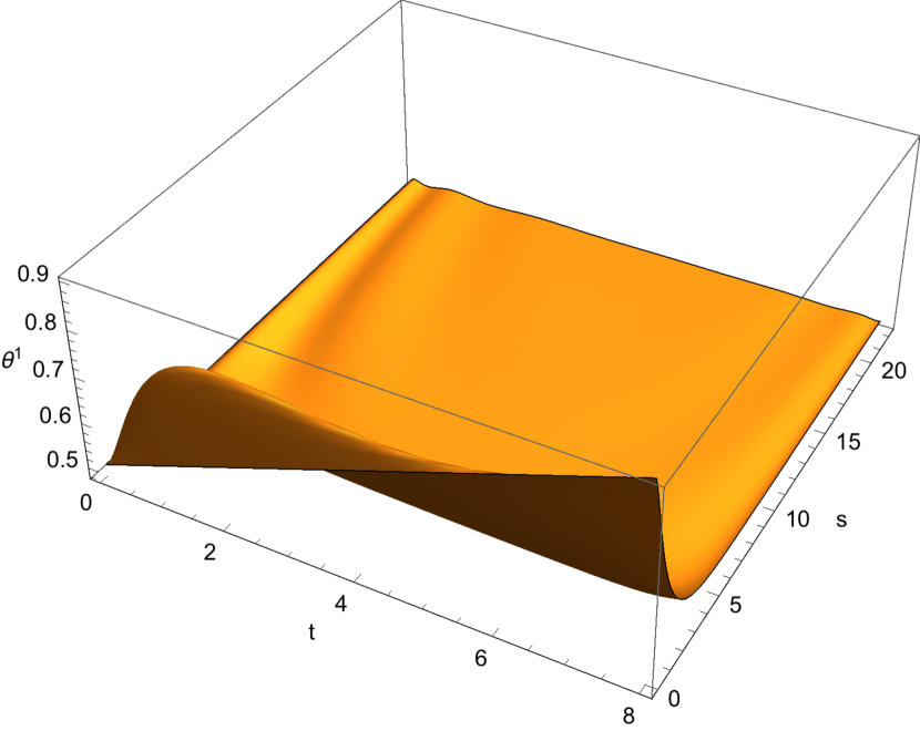
(a) Distribution of players $\theta^{1}(t,s)$.

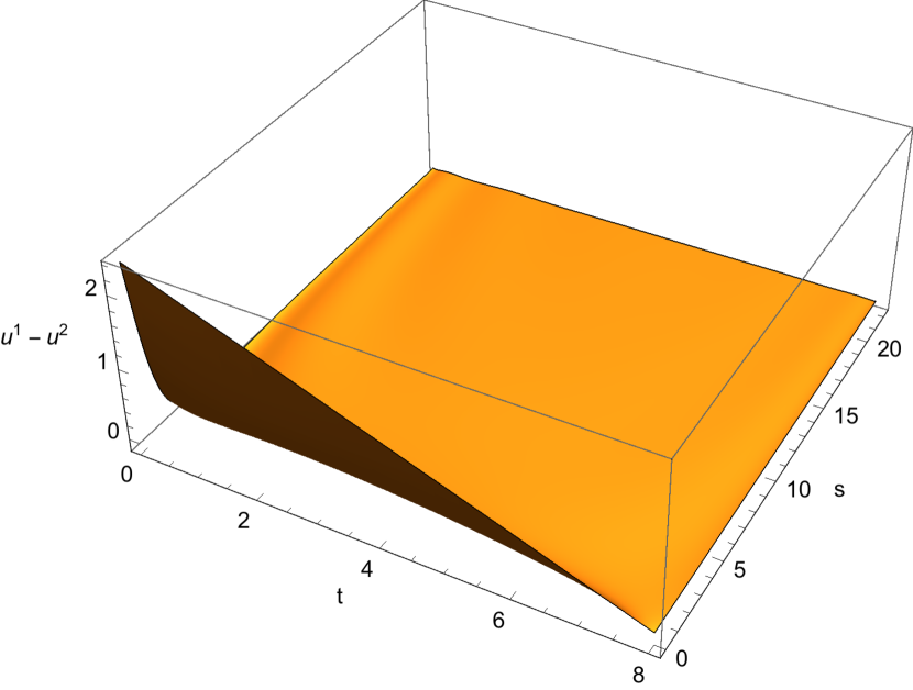
(b) Value functions $u(t,s)$.

Fig. 6. Evolution of $(u^{1}-u^{2})(\cdot,s)$ and $\theta(\cdot,s)$, for $s\in[0,20]$.

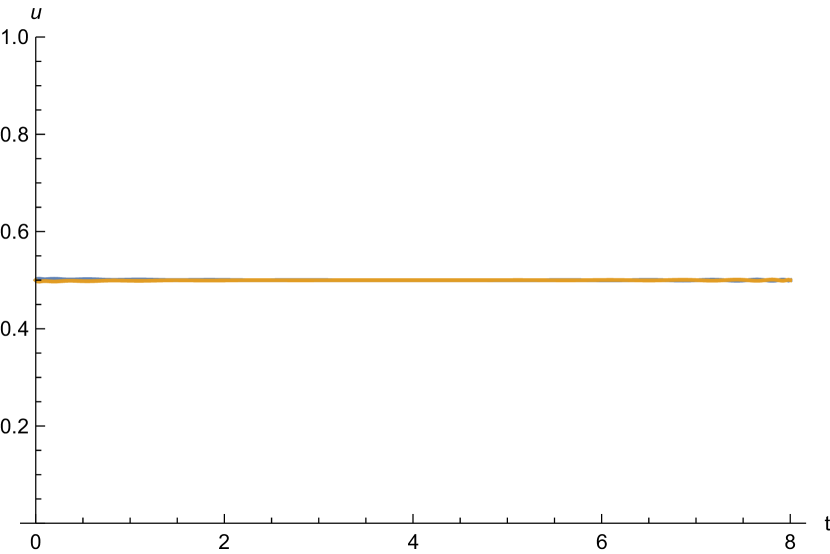
(a) Final distribution $\theta(\cdot,s=100)$.

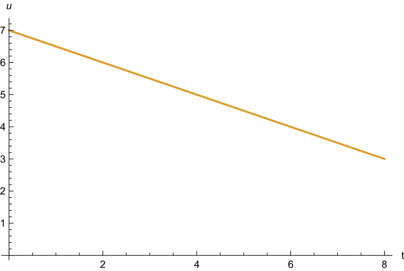
(b) Final value function $u(\cdot,s=100)$.

Fig. 7. Final value of $u(\cdot,s)$ and $\theta(\cdot,s)$, for $s=100$.

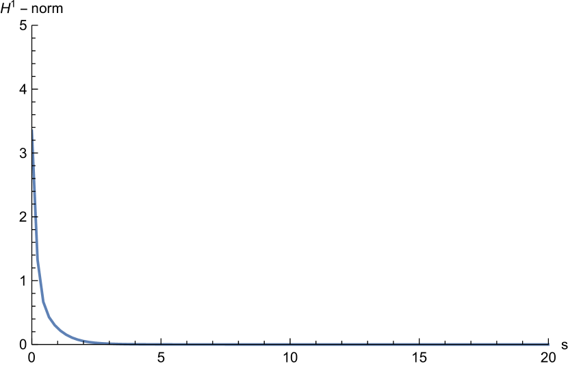
Fig. 8. Evolution, with the parameter $s$, of the $H^{1}$-norm of the difference between the computed solution $(u,\theta)(\cdot,s)$ and the analytical solution for the unconstrained probability case.

The paradigm-shift problem is a potential MFG with the Hamiltonian corresponding to

$$\tilde{h}(\Delta_{i}u,i)=-\frac{1}{2}((u^{i}-u^{j})^{+})^{2},\text{ and }F(\theta)=\frac{\theta_{1}^{2}+\theta_{2}^{2}}{2}$$

in (12). Thus, as a final test to our numerical method, we investigate the evolution of the Hamiltonian. In this case, as expected, the Hamiltonian converges to a constant, see Figure 9.

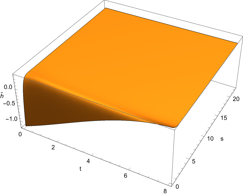
Fig. 9. Evolution of the Hamiltonian for $0\leq s\leq 20$.

In the preceding example, while iterating (52), $\theta$ remains away from $0$. In the next example, we consider a problem where, without the projection $P$ in (52), positivity is not preserved. We set $N=500$ and chose initial conditions as in Figure 10.

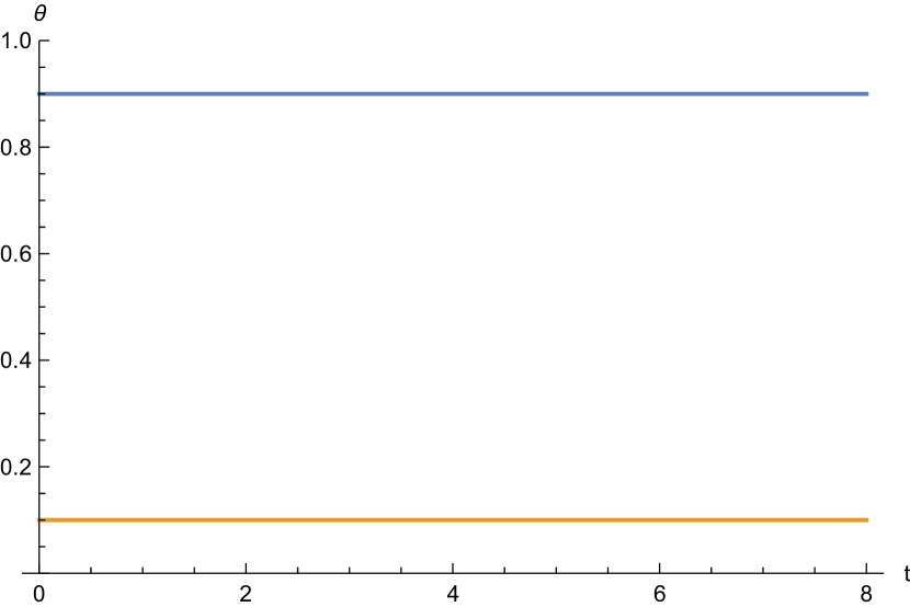
(a) Initial condition $\theta(\cdot,s=0)$.

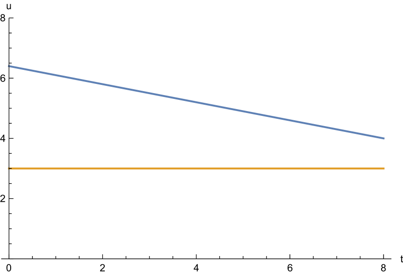
(b) Initial condition $u(\cdot,s=0)$.

Fig. 10. The blue lines correspond to the initial values ($s=0$) for state 1, $(\theta^{1},u^{1})$, the orange lines to the initial values for state 2, $(\theta^{2},u^{2})$.

In Figure 11, we show the evolution by (52) for $s\in[0,20]$. In Figure 12, we see the final result for $s=100$. Finally, in Figure 13, we show the evolution of the $H^{1}$ norm of the difference $\|(\tilde{u},\tilde{\theta})-(u,\theta)\|_{H^{1}([0,T])}^{2}(s)$, for $s\in[0,50]$.

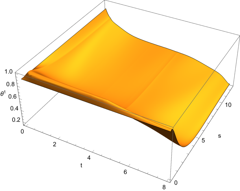
(a) Distribution of players $\theta^{1}$, at each time $t$.

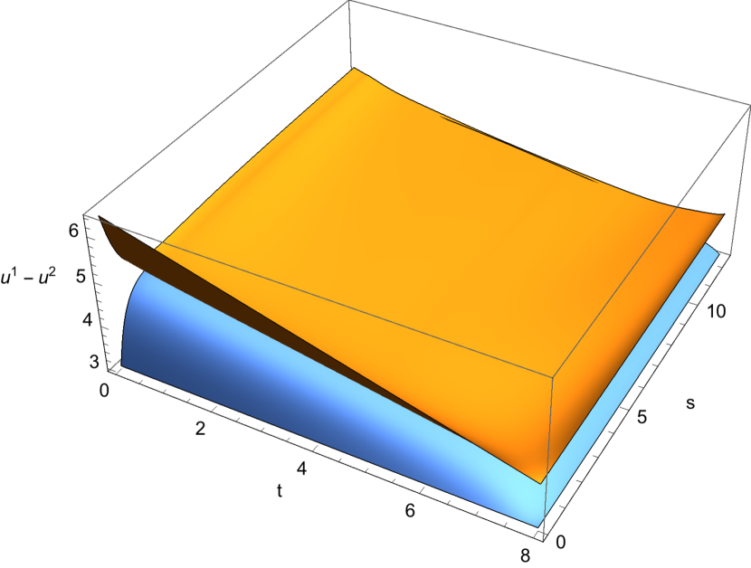
(b) Value functions $u^{1}$, and $u^{2}$.

Fig. 11. Evolution of $u(\cdot,s)$ and $\theta(\cdot,s)$, for $s\in[0,20]$. The quantities for the state 1 are depicted in blue and for state 2 in orange.

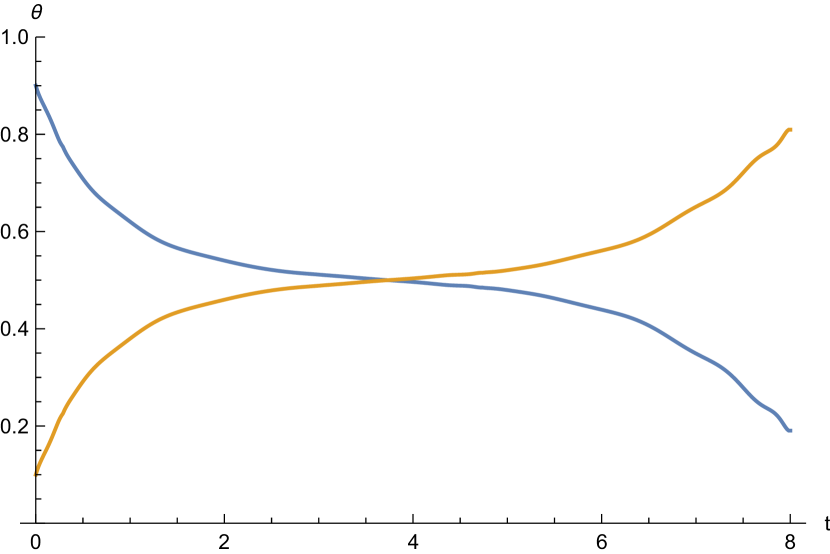
(a) Final distribution of players $\theta(\cdot,100)$.

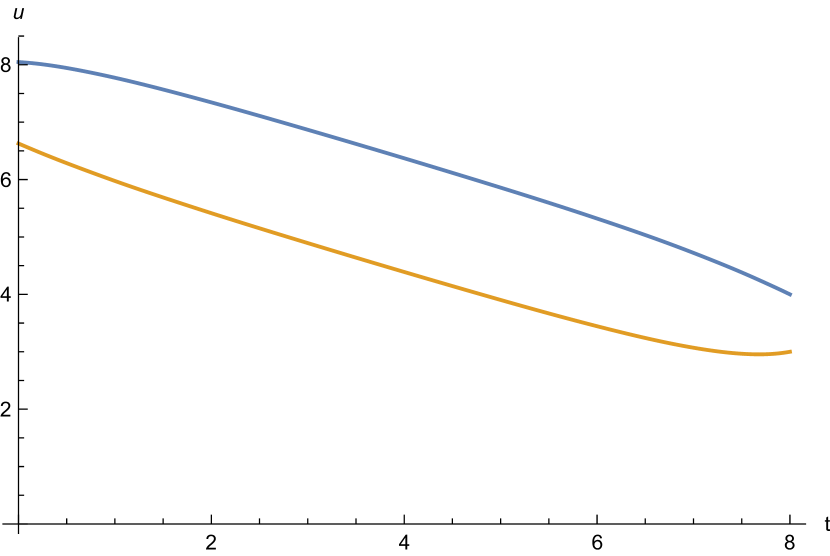
(b) Final value functions $u(\cdot,100)$.

Fig. 12. Final value of $u(\cdot,s)$ and distribution $\theta(\cdot,s)$, at $s=100$.

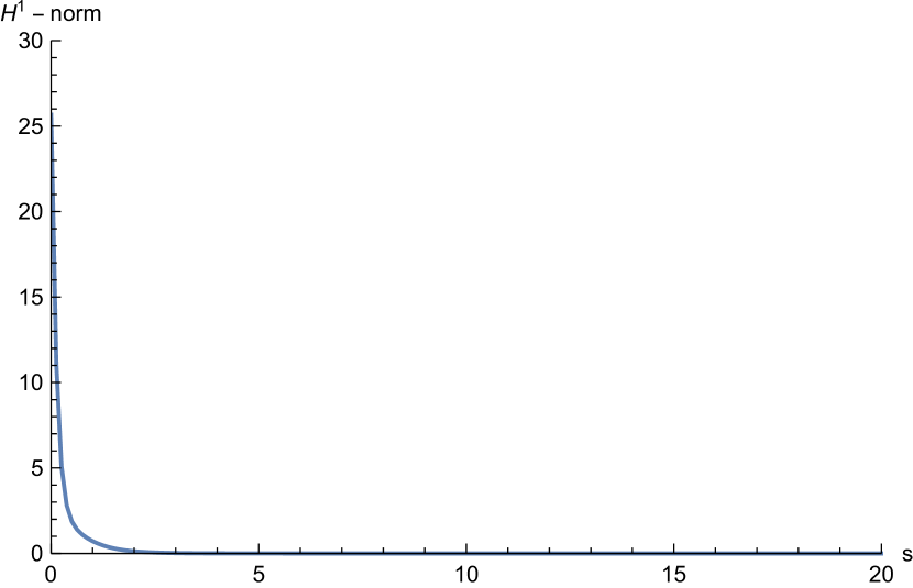
Fig. 13. Evolution, with respect to the parameter $s$, of the $H^{1}$-norm of the difference of the solution $(u,\theta)(\cdot,s)$ and the solution obtained at $s=100$: $\|(u,\theta)(\cdot,s)-(u,\theta)(\cdot,100)\|_{H^{1}}$.

In Figure 14, we plot the evolution of the Hamiltonian for using the projection method. Again, we obtain the numerical conservation of the Hamiltonian.

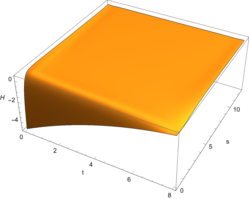
Fig. 14. Evolution of the Hamiltonian with the $s$-dynamics that preserves the probability and the positivity of the distribution of players.

5. Conclusions

As the examples in the preceding sections illustrate, we have developed an effective method for the numerical approximation of monotonic finite-state MFGs. As observed previously, [5, 1, 4, 3], monotonicity properties are essential for the construction of effective numerical methods and were used explicitly in [6]. Here, in contrast with earlier approaches, we do not use a Newton-type iteration as in [1, 4] nor require the solution of the master equation as in [21], which is numerically prohibitive for a large number of states. The key contribution of this work is the projection method developed in the previous section that made it possible to address the initial-terminal value problem. This was an open problem since the introduction of monotonicity-based methods in [6]. Our methods can be applied to discretize continuous-state MFGs, and we foresee additional extensions. The first one concerns the planning problem considered in [3]. A second extension regards boundary value problems, which are natural in many applications of MFGs. Finally, our methods may be improved by using higher-order integrators in time, provided monotonicity is preserved. These matters will be the subject of further research.

References

- [1] Y. Achdou. Finite difference methods for mean field games. In Hamilton-Jacobi Equations: Approximations, Numerical Analysis and Applications, pages 1–47. Springer, 2013.
- [2] Y. Achdou, M. Bardi, and M. Cirant. Mean field games models of segregation. Math. Models Methods Appl. Sci., 27(1):75–113, 2017.
- [3] Y. Achdou, F. Camilli, and I. Capuzzo-Dolcetta. Mean field games: numerical methods for the planning problem. SIAM J. Control Optim., 50(1):77–109, 2012.
- [4] Y. Achdou and I. Capuzzo-Dolcetta. Mean field games: numerical methods. SIAM J. Numer. Anal., 48(3):1136–1162, 2010.
- [5] Y. Achdou and V. Perez. Iterative strategies for solving linearized discrete mean field games systems. Netw. Heterog. Media, 7(2):197–217, 2012.
- [6] N. Al-Mulla, R. Ferreira, and D. Gomes. Two numerical approaches to stationary mean-field games. Preprint.
- [7] R. Basna, A. Hilbert, and V. N. Kolokoltsov. An epsilon-Nash equilibrium for non-linear Markov games of mean-field-type on finite spaces. Commun. Stoch. Anal., 8(4):449–468, 2014.
- [8] D Besancenot and H. Dogguy. Paradigm shift: a mean-field game approach. Bull. Econ. Res., 138, 2014.
- [9] L.M. Briceño Arias, D. Kalise, and F. J. Silva. Proximal methods for stationary mean field games with local couplings. Preprint.
- [10] P. Cardaliaguet, J.-M. Lasry, P.-L. Lions, and A. Porretta. Long time average of mean field games. Netw. Heterog. Media, 7(2):279–301, 2012.
- [11] P. Cardaliaguet, J-M. Lasry, P-L. Lions, and A. Porretta. Long time average of mean field games with a nonlocal coupling. SIAM Journal on Control and Optimization, 51(5):3558–3591, 2013.
- [12] E. Carlini and F. J. Silva. A fully discrete semi-Lagrangian scheme for a first order mean field game problem. SIAM J. Numer. Anal., 52(1):45–67, 2014.
- [13] E. Carlini and F. J. Silva. A semi-Lagrangian scheme for a degenerate second order mean field game system. Discrete Contin. Dyn. Syst., 35(9):4269–4292, 2015.
- [14] R. Ferreira and D. Gomes. Existence of weak solutions for stationary mean-field games through variational inequalities. Preprint.
- [15] R. Ferreira and D. Gomes. On the convergence of finite state mean-field games through -convergence. J. Math. Anal. Appl., 418(1):211–230, 2014.
- [16] D. Gomes, J. Mohr, and R. R. Souza. Discrete time, finite state space mean field games. Journal de Mathématiques Pures et Appliquées, 93(2):308–328, 2010.
- [17] D. Gomes, J. Mohr, and R. R. Souza. Continuous time finite state mean-field games. Appl. Math. and Opt., 68(1):99–143, 2013.
- [18] D. Gomes, E. Pimentel, and V. Voskanyan. Regularity theory for mean-field game systems. SpringerBriefs in Mathematics. Springer, [Cham], 2016.
- [19] D. Gomes and J. Saúde. Mean field games models—a brief survey. Dyn. Games Appl., 4(2):110–154, 2014.
- [20] D. Gomes, R. M. Velho, and M.-T. Wolfram. Dual two-state mean-field games. Proceedings CDC 2014, 2014.
- [21] Diogo A. Gomes, Roberto M. Velho, and Marie-Therese Wolfram. Socio-economic applications of finite state mean field games. 03 2014.
- [22] O. Guéant. An existence and uniqueness result for mean field games with congestion effect on graphs. Preprint, 2011.
- [23] O. Guéant. From infinity to one: The reduction of some mean field games to a global control problem. Preprint, 2011.
- [24] M. Huang, P. E. Caines, and R. P. Malhamé. Large-population cost-coupled LQG problems with nonuniform agents: individual-mass behavior and decentralized -Nash equilibria. IEEE Trans. Automat. Control, 52(9):1560–1571, 2007.
- [25] M. Huang, R. P. Malhamé, and P. E. Caines. Large population stochastic dynamic games: closed-loop McKean-Vlasov systems and the Nash certainty equivalence principle. Commun. Inf. Syst., 6(3):221–251, 2006.
- [26] J.-M. Lasry and P.-L. Lions. Jeux à champ moyen. I. Le cas stationnaire. C. R. Math. Acad. Sci. Paris, 343(9):619–625, 2006.
- [27] J.-M. Lasry and P.-L. Lions. Jeux à champ moyen. II. Horizon fini et contrôle optimal. C. R. Math. Acad. Sci. Paris, 343(10):679–684, 2006.
- [28] A. Mészáros and F. J. Silva. On the variational formulation of some stationary second order mean field games systems. Preprint.
- [29] A. Mészáros and F. J. Silva. A variational approach to second order mean field games with density constraints: the stationary case. J. Math. Pures Appl. (9), 104(6):1135–1159, 2015.