Second-kind integral equations for the Laplace-Beltrami problem on surfaces in three dimensions

Abstract

The Laplace-Beltrami problem $\Delta_{\Gamma}\psi=f$ has several applications in mathematical physics, differential geometry, machine learning, and topology. In this work, we present novel second-kind integral equations for its solution which obviate the need for constructing a suitable parametrix to approximate the in-surface Green’s function. The resulting integral equations are well-conditioned and compatible with standard fast multipole methods and iterative linear algebraic solvers, as well as more modern fast direct solvers. Using layer-potential identities known as Calderón projectors, the Laplace-Beltrami operator can be pre-conditioned from the left and/or right to obtain second-kind integral equations. We demonstrate the accuracy and stability of the scheme in several numerical examples along surfaces described by curvilinear triangles.

1   Introduction

For a smooth, closed surface $\Gamma$ embedded in $\mathbb{R}^{3}$, the Laplace-Beltrami problem

$$\Delta_{\Gamma}\psi=f$$ (1.1)

has numerous applications in partial differential equations [21, 51, 48], topology [44] and differential geometry [40], shape optimization [50], computer graphics [14], and even machine learning [54, 6]. The main application area in mind for this work is that of electromagnetics, where it is often useful to partition tangential vector fields (e.g. electric current) on surfaces of arbitrary genus into their Hodge decomposition [21, 22]. The Hodge decomposition is the generalization of the standard Helmholtz decomposition to multiply-connected domains, and allows for a component of the vector field which is divergence and curl free. In particular, any tangential vector field $\bm{F}$ along a smooth, closed surface $\Gamma$ can be written as

$$\bm{F}=\nabla_{\Gamma}\alpha+\bm{n}\times\nabla_{\Gamma}\beta+\bm{H},$$ (1.2)

where $\nabla_{\Gamma}$ denotes the surface gradient, $\alpha$, $\beta$ are functions defined along $\Gamma$, and $\bm{n}$ is the unit normal vector. (In what follows, we will restrict our discussion and applications to smooth vector fields $\bm{F}$.) The surface divergence is denoted by $\nabla_{\Gamma}\cdot$, and the surface curl is given by $\nabla_{\Gamma}\cdot(\bm{n}\times)$ so that

$$\nabla_{\Gamma}\cdot\bm{F}=\Delta_{\Gamma}\alpha,\qquad\nabla_{\Gamma}\cdot(\bm{n}\times\bm{F})=-\Delta_{\Gamma}\beta.$$ (1.3)

The vector field $\bm{H}$ is the harmonic component of $\bm{F}$, and has zero divergence and curl:

$$\nabla_{\Gamma}\cdot\bm{H}=0,\qquad\nabla_{\Gamma}\cdot(\bm{n}\times\bm{H})=0.$$ (1.4)

The existence of non-trivial vector fields $\bm{H}$ depends on the genus of $\Gamma$: the dimension of this harmonic subspace is $2p$, with $p$ denoting the genus of $\Gamma$. The exact usefulness of this decomposition with regard to problems in electromagnetics is discussed in detail in [21, 22, 23, 18]. To summarize one particular application, electromagnetic fields in the exterior of a perfect electric conductor (PEC) with smooth boundary $\Gamma$ can be represented using what are known as generalized Debye sources, denoted below by $r$, $q$. After sufficient scaling, the time-harmonic Maxwell equations with wavenumber $k$ in a source and current free region can be written as [43]:

$$\nabla\times\bm{E} =ik\bm{B}, \qquad\nabla\times\bm{B} =-ik\bm{E},$$ (1.5)

$$\nabla\cdot\bm{E} =0, \nabla\cdot\bm{B} =0.$$

With the above standardization, the electric and magnetic fields in the exterior of a PEC can be represented as

$$\bm{E} =ik\mathcal{S}_{k}\bm{J}-\nabla\mathcal{S}_{k}r-\nabla\times\mathcal{S}_{k}\bm{K},$$ (1.6)

$$\bm{B} =ik\mathcal{S}_{k}\bm{K}-\nabla\mathcal{S}_{k}q+\nabla\times\mathcal{S}_{k}\bm{J},$$

where $k$ is the wavenumber of the fields and $\mathcal{S}_{k}$ is the single-layer Helmholtz operator:

$$\mathcal{S}_{k}f(\bm{x})=\int_{\Gamma}\frac{e^{ik|\bm{x}-\bm{x}^{\prime}|}}{4\pi|\bm{x}-\bm{x}^{\prime}|}\,f(\bm{x}^{\prime})\,da(\bm{x}^{\prime}).$$ (1.7)

The surface vector fields $\bm{J}$ and $\bm{K}$ are defined using $r$, $q$ in Hodge form so that $\bm{E}$, $\bm{B}$ in (1.6) automatically satisfy Maxwell’s equations:

$$\bm{J} =ik\left(\nabla_{\Gamma}\Delta_{\Gamma}^{-1}r-\bm{n}\times\nabla_{\Gamma}\Delta_{\Gamma}^{-1}q\right)+\bm{J}_{H},$$ (1.8)

$$\bm{K} =\bm{n}\times\bm{J},$$

where $\bm{J}_{H}$ is a harmonic vector field along $\Gamma$. Note that the construction of $\bm{J}$ and $\bm{K}$ requires the application of $\Delta_{\Gamma}^{-1}$ (or, equivalently, the solution of $\Delta_{\Gamma}\psi=r$).

Despite the many applications of the Laplace-Beltrami problem in widely varying domains, the literature surrounding its numerical solution is rather limited. Methods which directly discretize the differential operator are usually based on finite elements or finite differences [8, 30, 19, 20, 26]. Alternatively, there are a few methods [36, 37] relevant to problems along surfaces in three dimensions which re-formulate the problem in integral form using a parametrix of $\log$-type, which to leading order, is the Green’s function for $\Delta_{\Gamma}$ on surfaces embedded in three dimensions. Integral equations on surfaces in three dimensions is a well-studied field [34], but usually the kernels involved are Green’s functions corresponding to constant-coefficient PDEs in three dimensions, and not variable coefficient ones along two-dimensional surfaces. Outside of special-case geometries, novel quadrature rules and fast algorithms would need to be constructed in order to rapidly solve integral equations on surfaces in three dimensions with logarithmically-singular kernels.

If one is willing to obtain or construct a signed distance function (defined in the volume) to the surface $\Gamma$, then various level-set methods become options for solving surface PDEs, including the Laplace-Beltrami problem. This approach was taken in [7, 29, 15, 39, 38, 46] for 2nd-order and 4th-order surface diffusion-type problems, including the Cahn-Hilliard equation. These schemes are based on using an embedded finite difference scheme (in the volume) to discretize an extension of the surface PDE (often using formulas such as (2.10), below). While very general (and very efficient yielding sparse matrices to invert), and certainly applicable to a wide range of surface PDEs, the solvers associated with level set methods and the closest point method can suffer from ill-conditioning in the presence of adaptive discretizations (possibly needed in order to resolve sharp geometric features or high-bandwidth right-hand sides). Furthermore, methods based on such volumetric extensions inherently require extending the right-hand side from the surface to the volume, which is a notoriously difficult task to do with high-order accuracy [3].

With this in mind, in this work we introduce special-purpose, second-kind boundary integral equations obtained by applying left- and right-preconditioners to the Laplace-Beltrami problem that can be used for its efficient solution. The resulting integral equations rely on several Calderón identities for harmonic layer potentials, and contain integral operators whose kernel is the Green’s function for the three-dimensional Laplacian. These features allow for the immediate use of fast algorithms, such as fast multipole methods (FMMs) [28], and standard quadrature methods for weakly singular integrals along surfaces [10, 11]. We will demonstrate the effectiveness of these integral equations with several numerical examples.

The paper is organized as follows: In Section 2 we introduce the Laplace-Beltrami operator and provide some standard relationships with the three-dimensional Laplacian. In Section 3 we derive novel second-kind integral equations useful in solving the Laplace-Beltrami problem. In Section 4 we describe the numerical discretization of arbitrary curvilinear surfaces and derive various quantities from differential geometry. Section 5 contains several examples of the resulting solver, and finally in Section 6 , we discuss advantages, drawbacks, and future improvements of our scheme.

2   The Laplace-Beltrami operator

The Laplace-Beltrami operators, also known as the surface Laplacian, is the generalization of the Laplace operator to general curvilinear coordinates. In what follows, we will always assume that the surface $\Gamma$ has at least two continuous derivatives, and in practice, we provide examples which have higher degrees of smoothness. For a surface $\Gamma$ parameterized (at least locally) by a smooth function $\bm{x}:\mathbb{R}^{2}\to\mathbb{R}^{3}$,

$$\bm{x}(u,v)=x_{1}(u,v)\,\mathbf{e}_{1}+x_{2}(u,v)\,\mathbf{e}_{2}+x_{3}(u,v)\,\mathbf{e}_{3},$$ (2.1)

where $\mathbf{e}_{1}$, $\mathbf{e}_{2}$, $\mathbf{e}_{3}$ is the elementary orthonormal basis for $\mathbb{R}^{3}$, the metric tensor is given by

$$g=\begin{pmatrix}\bm{x}_{u}\cdot\bm{x}_{u}&\bm{x}_{u}\cdot\bm{x}_{v}\\ \bm{x}_{v}\cdot\bm{x}_{u}&\bm{x}_{v}\cdot\bm{x}_{v}\end{pmatrix}.$$ (2.2)

The determinant of the metric tensor will be denoted as $\det g=|g|$, and the components of $g$ as:

$$g_{uu} =\bm{x}_{u}\cdot\bm{x}_{u}, \qquad g_{uv} =\bm{x}_{u}\cdot\bm{x}_{v},$$ (2.3)

$$g_{vu} =\bm{x}_{v}\cdot\bm{x}_{u}, \quad g_{vv} =\bm{x}_{v}\cdot\bm{x}_{v}.$$

Here, we use the abbreviations $\bm{x}_{u}=\partial\bm{x}/\partial u$ and $\bm{x}_{v}=\partial\bm{x}/\partial v$. The unit outward normal vector is given by

$$\bm{n}(\bm{x})=\frac{\bm{x}_{u}\times\bm{x}_{v}}{|\bm{x}_{u}\times\bm{x}_{v}|}$$ (2.4)

so that the vectors $\bm{x}_{u}$, $\bm{x}_{v}$, and $\bm{n}$ form a right-handed system of coordinates. The surface divergence and gradient are then [25, 41]:

$$\nabla_{\Gamma}\cdot\bm{F} =\frac{1}{\sqrt{|g|}}\left(\frac{\partial}{\partial u}\left(\sqrt{|g|}\,F^{u}\right)+\frac{\partial}{\partial v}\left(\sqrt{|g|}\,F^{v}\right)\right),$$ (2.5)

$$\nabla_{\Gamma}\psi =\left(g^{uu}\frac{\partial\psi}{\partial u}+g^{uv}\frac{\partial\psi}{\partial v}\right)\bm{x}_{u}+\left(g^{vu}\frac{\partial\psi}{\partial u}+g^{vv}\frac{\partial\psi}{\partial v}\right)\bm{x}_{v},$$

where $\psi=\psi(u,v)$ is a scalar function along $\Gamma$, $\bm{F}=\bm{F}(u,v)$ is a tangential vector field defined with respect to the tangent vectors $\bm{x}_{u}$ and $\bm{x}_{v}$:

$$\bm{F}(u,v)=F^{u}(u,v)\,\bm{x}_{u}+F^{v}(u,v)\,\bm{x}_{v},$$ (2.6)

and the coefficients $g^{ij}$ are the components of the inverse of $g$:

$$g^{-1}=\begin{pmatrix}g^{uu}&g^{uv}\\ g^{vu}&g^{vv}\end{pmatrix}.$$ (2.7)

If the surface $\Gamma$ is closed, the surface gradient and divergence yield the integration by parts formula:

$$\int_{\Gamma}\nabla_{\Gamma}\psi\cdot\bm{F}\,da=-\int_{\Gamma}\psi\,\nabla_{\Gamma}\cdot\bm{F}\,da,$$ (2.8)

where $da=\sqrt{|g|}\,du\,dv$ is the surface-area differential. The Laplace-Beltrami operator is then defined as $\Delta_{\Gamma}=\nabla_{\Gamma}\cdot\nabla_{\Gamma}$, and given explicitly as:

$$\Delta_{\Gamma}\psi=\frac{1}{\sqrt{|g|}}\left(\frac{\partial}{\partial u}\sqrt{|g|}\left(g^{uu}\,\frac{\partial\psi}{\partial u}+g^{uv}\,\frac{\partial\psi}{\partial v}\right)+\frac{\partial}{\partial v}\sqrt{|g|}\left(g^{vu}\,\frac{\partial\psi}{\partial u}+g^{vv}\,\frac{\partial\psi}{\partial v}\right)\right).$$ (2.9)

From the previous definition of the Laplace-Beltrami operator, it is clear that in general, the problem of solving $\Delta_{\Gamma}\psi=f$ requires solving a second-order variable-coefficient PDE in the variables $u$, $v$. Solutions of this variable coefficient PDE can be obtained via pseudo-spectral methods if a tractable parameterization of the boundary can be obtained [31] or by finite differences or finite element methods [8, 20]. In each of these cases, complicated geometry plays a key role. The goal of this paper will be to avoid designing methods for variable coefficient PDEs along surfaces, and instead obtain an equivalent well-conditioned linear integral equation compatible with existing fast algorithms that can be used to solve the Laplace-Beltrami problem.

Alternatively, for functions defined not just along $\Gamma$, but in a neighborhood of $\Gamma$, the surface Laplacian can be written in terms of the standard three-dimensional Laplacian plus correction terms which remove differential contributions in the normal direction. See, for example, [41] for a derivation of the following lemma.

Lemma 2.1.

For an object $\Omega$ in three dimensions with smooth boundary given by $\Gamma$ and a twice differentiable function $\psi=\psi(\bm{x})$ defined in a neighborhood of $\Gamma$, we have that

$$\Delta\psi=\Delta_{\Gamma}\psi+2H\frac{\partial\psi}{\partial n}+\frac{\partial^{2}\psi}{\partial n^{2}},$$ (2.10)

where $H$ is the signed mean curvature,

$$H=\frac{\nabla\cdot\bm{n}}{2},$$ (2.11)

and $\partial/\partial n$ denotes differentiation in the direction normal (outward) to the boundary of $\Omega$:

$$\frac{\partial\psi}{\partial n}=\bm{n}\cdot\nabla\psi.$$ (2.12)

Note that in the previous lemma, we have defined the mean curvature $H$ so that the unit sphere has $H=1$, assuming that the outward normal is given by $\bm{n}=\bm{r}$. The following corollary addresses the case in which the function $\psi$ is harmonic.

Corollary 2.2.

If the function $\psi$ defined in Lemma 2.1 is also harmonic in the neighborhood of $\Gamma$, then we have that

$$\Delta_{\Gamma}\psi=-2H\frac{\partial\psi}{\partial n}-\frac{\partial^{2}\psi}{\partial n^{2}}.$$ (2.13)

Finally, we conclude this section with a brief discussion of the invertibility of the Laplace-Beltrami operator. Clearly, $\Delta_{\Gamma}$ contains a nullspace of dimension one, namely that of constant functions along $\Gamma$. Therefore, in order to formulate a well-posed Laplace-Beltrami problem, we must restrict the operator, and its inverse, to mean-zero functions (or enforce some other constraint). The following lemma is a standard result in Hodge theory, and discussed in more detail in [41, 21].

Lemma 2.3.

For smooth closed boundaries $\Gamma$, the Laplace-Beltrami operator is uniquely invertible as a map from $\mathcal{M}_{0}$ to $\mathcal{M}_{0}$, the space of mean-zero functions defined on $\Gamma$:

$$\mathcal{M}_{0}=\left\{\psi:\int_{\Gamma}\psi\,da=0\right\}.$$ (2.14)

That is to say, for a function $f\in\mathcal{M}_{0}$, there is a unique twice-differentiable $\psi\in\mathcal{M}_{0}$ such that $\Delta_{\Gamma}\psi=f$. In what follows in this section and all subsequent ones, we will assume that the right hand side of the Laplace-Beltrami equation, $f$, is a continuous function in $L^{2}(\Gamma)$ in order to avoid a discussion of singular layer potential densities. We now have that the following PDE + constraint is a well-posed system:

$$\Delta_{\Gamma}\psi =f\qquad\text{on }\Gamma,$$ (2.15)

$$\int_{\Gamma}\psi =0.$$

Given these facts regarding the Laplace-Beltrami operator, we now turn to deriving integral equations for its solution.

3   Integral equation formulations

In this section, we derive second-kind integral equations which can be used to solve the Laplace-Beltrami problem along smooth surfaces in three dimensions. These integral equations rely only on standard layer potentials, their normal derivatives, and local curvature information of $\Gamma$. The resulting solvers are immediately compatible with standard fast algorithms and iterative solvers (e.g. FMMs and GMRES [47]). The main working tool of the following derivation will be what are known as Calderón identities, which we discuss now.

3.1   Calderón projectors

In order to derive well-conditioned second-kind integral equations for the Laplce-Beltrami equation along surfaces, it is useful to precondition equation (1.1) (on both the left and the right) and invoke what are known as Calderón relations (also known as identities or projections) to rewrite the resulting operator in diagonal and compact terms. To this end, we briefly provide several Calderón identities that will be useful. These identities, and simple proofs using only standard Green’s identities, can be found in [41].

Let us denote by $G$ the Green’s function for the Laplace equation in three dimensions:

$$G(\bm{x}-\bm{x}^{\prime})=\frac{1}{4\pi|\bm{x}-\bm{x}^{\prime}|}.$$ (3.1)

This Green’s function satisfies $\Delta_{\bm{x}}G(\bm{x}-\bm{x}^{\prime})=-\delta(\bm{x}-\bm{x}^{\prime})$, where $\delta$ is the Dirac delta function defined in the proper sense of distributions [24], and $\Delta_{\bm{x}}$ denotes the Laplacian applied in the $\bm{x}$ variable. For $\bm{x}\notin\Gamma$, we next denote by $\mathcal{S}$ and $\mathcal{D}$ the standard single- and double-layer potential operators for Laplace potentials, given by:

$$\mathcal{S}\sigma(\bm{x})=\int_{\Gamma}G(\bm{x}-\bm{x}^{\prime})\,\sigma(\bm{x}^{\prime})\,da(\bm{x}^{\prime}),\qquad\mathcal{D}\sigma(\bm{x})=\int_{\Gamma}\left(\frac{\partial}{\partial n^{\prime}}G(\bm{x}-\bm{x}^{\prime})\right)\sigma(\bm{x}^{\prime})\,da(\bm{x}^{\prime}),$$ (3.2)

with $\partial/\partial n^{\prime}=\bm{n}^{\prime}\cdot\nabla_{\bm{x}^{\prime}}$ denoting differentiation in the direction normal to the surface at $\bm{x}^{\prime}$. The functions $\mathcal{S}\sigma$ and $\mathcal{D}\sigma$ define smooth functions up to $\Gamma$; $\mathcal{S}\sigma$ is continuous across the boundary $\Gamma$, while $\mathcal{D}\sigma$ has a jump of size $\sigma$ across $\Gamma$. In particular, for $\bm{x}\in\Gamma$

$$\lim_{h\to 0^{\pm}}\mathcal{D}\sigma(\bm{x}+h\bm{n})=\pm\frac{\sigma(\bm{x})}{2}+\mathcal{D}\sigma(\bm{x}).$$ (3.3)

One-sided normal derivatives of the layer potentials $\mathcal{S}\sigma$ and $\mathcal{D}\sigma$ can also be taken. For $\bm{x}\in\Gamma$, we have

$$\lim_{h\to 0^{\pm}}\frac{\partial}{\partial n}\mathcal{S}\sigma(\bm{x}+h\bm{n}) =\mp\frac{\sigma(\bm{x})}{2}+\mathcal{S}^{\prime}\sigma(\bm{x}),$$ (3.4)

$$\lim_{h\to 0^{\pm}}\frac{\partial}{\partial n}\mathcal{D}\sigma(\bm{x}+h\bm{n}) =\mathcal{D}^{\prime}\sigma(\bm{x}),$$

where the layer potential operators $\mathcal{S}^{\prime}$ and $\mathcal{D}^{\prime}$, as maps from $\Gamma\to\Gamma$, are given by:

$$\mathcal{S}^{\prime}\sigma(\bm{x})=\int_{\Gamma}\left(\frac{\partial}{\partial n}G(\bm{x}-\bm{x}^{\prime})\right)\sigma(\bm{x}^{\prime})\,da(\bm{x}^{\prime}),\qquad\mathcal{D}^{\prime}\sigma(\bm{x})=\int_{\Gamma}\left(\frac{\partial^{2}}{\partial n\,\partial n^{\prime}}G(\bm{x}-\bm{x}^{\prime})\right)\sigma(\bm{x}^{\prime})\,da(\bm{x}^{\prime}).$$ (3.5)

The function $\mathcal{D}^{\prime}\sigma$ is continuous across the interface, while $\mathcal{S}\sigma$ has a jump in its normal derivative. The kernel in $\mathcal{D}^{\prime}$ is, however, not integrable and therefore the integral is interpreted in Hadamard finite-parts [41, 34, 16].

Next, define the matrix $\mathcal{P}$ of operators from $\Gamma\times\Gamma\to\Gamma\times\Gamma$ by

$$\mathcal{P}=\begin{pmatrix}\mathcal{D}&\mathcal{S}\\ -\mathcal{D}^{\prime}&-\mathcal{S}^{\prime}\end{pmatrix}.$$ (3.6)

This matrix has the projector-like quality (on $\Gamma$) that $\mathcal{P}^{2}=\mathcal{I}/4$, where $\mathcal{I}$ is the identity operator. This can be proven using a straightforward application of on-surface Green’s identities [41]. We then have the four following explicit relationships, known as Calderón identities:

$$\mathcal{D}\mathcal{D}-\mathcal{S}\mathcal{D}^{\prime} =\frac{\mathcal{I}}{4},\qquad \mathcal{D}\mathcal{S} =\mathcal{S}\mathcal{S}^{\prime},$$ (3.7)

$$\mathcal{S}^{\prime}\mathcal{S}^{\prime}-\mathcal{D}^{\prime}\mathcal{S} =\frac{\mathcal{I}}{4}, \mathcal{D}^{\prime}\mathcal{D} =\mathcal{S}^{\prime}\mathcal{D}^{\prime}.$$

These identities are very useful in constructing preconditioners for hypersingular integral equations [17] and integral equations for high-frequency acoustic scattering phenomena [9]. We will next use these relationships to construct integral equations for solving the Laplace-Beltrami equation.

3.2   Laplace-Beltrami integral equations

Using the Calderón identities of the previous section, we can now derive integral equations of the second-kind which can be used to solve the Laplace-Betrami problem. For example, letting $\psi=\mathcal{S}\sigma$ in equation (1.1) and preconditioning on the left yields:

$$\mathcal{S}\Delta_{\Gamma}\mathcal{S}\sigma=\mathcal{S}f,$$ (3.8)

which turns out to be a second-kind integral equation for the function $\sigma$. Once $\sigma$ has been found, the original function $\psi$ can be computed easily. To this end, we begin with the following lemma.

Lemma 3.1.

As a map from $\Gamma\to\Gamma$,

$$\mathcal{S}\Delta_{\Gamma}\mathcal{S}=-\frac{\mathcal{I}}{4}+\mathcal{D}^{2}-\mathcal{S}(\mathcal{S}^{\prime\prime}+\mathcal{D}^{\prime})-2\mathcal{S}H\mathcal{S}^{\prime},$$ (3.9)

where $H$ is the mean curvature of $\Gamma$ and the operator $\mathcal{S}^{\prime\prime}:\Gamma\to\Gamma$ is given by

$$\mathcal{S}^{\prime\prime}\sigma(\bm{x})=\int_{\Gamma}\left(\frac{\partial^{2}}{\partial n^{2}}G(\bm{x}-\bm{x}^{\prime})\right)\sigma(\bm{x}^{\prime})\,da(\bm{x}^{\prime}).$$ (3.10)

Proof.

For any $\sigma$ defined along $\Gamma$, the function $\mathcal{S}\sigma$ is infinitely differentiable off of $\Gamma$ and is continuous across $\Gamma$. Furthermore, it defines a harmonic function and therefore $\Delta\mathcal{S}\sigma=0$ along $\Gamma$. Using this fact, along with Lemma 2.1, we have that

$$\Delta_{\Gamma}\mathcal{S}=-2H\mathcal{S}^{\prime}-\mathcal{S}^{\prime\prime}.$$ (3.11)

The operator $\mathcal{S}^{\prime\prime}$ is interpreted in the finite-parts sense, as is $\mathcal{D}^{\prime}$. After applying $\mathcal{S}$ to both sides of equation (3.11), and adding/subtracting $\mathcal{S}\mathcal{D}^{\prime}$, we have:

$$\mathcal{S}\Delta_{\Gamma}\mathcal{S}=-2\mathcal{S}H\mathcal{S}^{\prime}-\mathcal{S}\left(\mathcal{S}^{\prime\prime}+\mathcal{D}^{\prime}\right)+\mathcal{S}\mathcal{D}^{\prime}.$$ (3.12)

Using the Calderón identity $\mathcal{S}\mathcal{D}^{\prime}=-\mathcal{I}/4+\mathcal{D}^{2}$ from (3.7), we have that

$$\mathcal{S}\Delta_{\Gamma}\mathcal{S}=-\frac{\mathcal{I}}{4}-2\mathcal{S}H\mathcal{S}^{\prime}-\mathcal{S}\left(\mathcal{S}^{\prime\prime}+\mathcal{D}^{\prime}\right)+\mathcal{D}^{2}.$$ (3.13)

The terms $\mathcal{S}H\mathcal{S}^{\prime}$ and $\mathcal{D}^{2}$ are trivially compact due to their weakly-singular kernels, and the difference operator $\mathcal{S}^{\prime\prime}+\mathcal{D}^{\prime}$ can also be shown to be compact by expressing its kernel as

$$K=\frac{\partial}{\partial n}\left(\frac{\partial G}{\partial n}+\frac{\partial G}{\partial n^{\prime}}\right).$$ (3.14)

As $\bm{x}\to\bm{x}^{\prime}$, the terms $\partial G/\partial n$ and $\partial G/\partial n^{\prime}$ cancel to leading order, and what remains after applying $\partial/\partial n$ is weakly singular. See [45, 35] for early uses of this fact. Therefore, (3.13) gives a second-kind integral operator formulation of the operator $\mathcal{S}\Delta_{\Gamma}\mathcal{S}$. ∎

The above identity is straightforward to verify on the unit sphere by using the diagonal forms of the layer potential operators when applied to spherical harmonics [52]. Alternatively, a different second-kind formulation exists which corresponds to a fully right-preconditioned system. We provide this formulation in the following lemma.

Lemma 3.2.

As a map from $\Gamma\to\Gamma$,

$$\Delta_{\Gamma}\mathcal{S}^{2}=-\frac{\mathcal{I}}{4}+\mathcal{S}^{\prime 2}-\left(\mathcal{S}^{\prime\prime}+\mathcal{D}^{\prime}\right)\mathcal{S}-2H\mathcal{S}^{\prime}\mathcal{S}$$ (3.15)

Proof.

The proof is similar to that of the previous lemma, and omitted here. ∎

The operator $\mathcal{S}^{2}$ behaves similarly to convolution with a logarithmic parametrix along $\Gamma$, and for this reason it is not surprising that the operator in equation (3.15) is Fredholm of the second-kind. In many respects, integral equation (3.9) and (3.15) behave identically. However, in practice we prefer equation (3.9) due to the fact that the right-hand side $f$ is smoothed by the application of $\mathcal{S}$, and therefore fewer discretization nodes are needed in order to resolve $\mathcal{S}f$ than are needed to resolve $f$.

Lastly, we discuss the invertibility of the integral operators (3.9) and (3.15). As shown in [31, 49], since the nullspace of the surface Laplacian is exactly one-dimensional (constant functions) and $\Delta_{\Gamma}$ is self-adjoint, letting the operator $\mathcal{W}$ be defined as

$$\mathcal{W}\psi=\int_{\Gamma}\psi\,da$$ (3.16)

we have that the integro-differentiable operator $\Delta_{\Gamma}+\mathcal{W}$ is of full rank, and uniquely invertible on the space of mean-zero functions. Therefore, the operators

$$\mathcal{S}\left(\Delta_{\Gamma}+\mathcal{W}\right)\mathcal{S},\qquad\text{and}\qquad\left(\Delta_{\Gamma}+\mathcal{W}\right)\mathcal{S}^{2}$$ (3.17)

are Fredholm operators of the second-kind, and uniquely invertible. The integral expressions for these operators can be obtained from the expressions in (3.9) and (3.15) with the addition of the terms $\mathcal{S}\mathcal{W}\mathcal{S}$ and $\mathcal{W}\mathcal{S}^{2}$, respectively.

4   Discretization of surfaces and layer potentials

Often the hardest part of any boundary integral equation method is not the fast algorithm used to invert the resulting linear system, but rather obtaining high-order descriptions of the geometry and building accurate methods with which to compute weakly-singular integrals. In this section we give a brief overview of the surface and density discretizations we use for subsequent numerical examples for solving the Laplace-Beltrami problem. Our solver relies on decoupling the surface description from the discretization of functions along the surface, and it is based on the one contained in [10, 11]. This allows for high-order discretizations of functions along low-order surfaces, and vice versa. While the overall order of the scheme is often limited by the lowest order of discretization (i.e. the geometry vs. the unknowns), it is useful for numerical experiments to have control over both orders.

4.1   Maps of standard triangles

We assume that our surface $\Gamma$ is given by a sequence of curvilinear triangles, each described as a smooth map of the standard simplex triangle, denoted by $T_{0}$, with vertices $\{(0,0),(1,0),(0,1)\}$. That is to say, the $j$th triangle along $\Gamma$ is parameterized by the map:

$$\bm{x}^{j}(u,v)=x^{j}_{1}(u,v)\,\mathbf{e}_{1}+x^{j}_{2}(u,v)\,\mathbf{e}_{2}+x^{j}_{3}(u,v)\,\mathbf{e}_{3},$$ (4.1)

with $\mathbf{e}_{1}$, $\mathbf{e}_{2}$, $\mathbf{e}_{3}$ the standard basis for $\mathbb{R}^{3}$. In the case of analytically parameterized surfaces, the functions $x^{j}_{i}$ are known globally, and in other (lower-order) cases, the surface maps may be provided triangle-by-triangle as piecewise polynomials:

$$x_{i}^{j}(u,v)=\sum_{m+n\leq p}c^{ji}_{mn}\,u^{m}\,v^{n},$$ (4.2)

with $p$ denoting the order of the discretization of $\Gamma$. In each case, local derivatives of the surface with respect to $u$ and $v$ can be computed analytically. Surface area elements can be computed using standard differential geometry formulas, as discussed in Section 2. The mean curvature at any point $\bm{x}(u,v)$ can be computed as

$$H=-\frac{1}{2}\operatorname{Tr}\left({II}\cdot{I}^{-1}\right),$$ (4.3)

with $I=g$ (the metric tensor) and $II$ the first and second fundamental forms, respectively [13]. The second fundamental form is defined as

$$II=\begin{pmatrix}\bm{x}_{uu}\cdot\bm{n}&\bm{x}_{uv}\cdot\bm{n}\\ \bm{x}_{vu}\cdot\bm{n}&\bm{x}_{vv}\cdot\bm{n}\end{pmatrix},$$ (4.4)

with

$$\bm{x}_{uu}=\frac{\partial^{2}\bm{x}}{\partial u^{2}},\qquad\bm{x}_{uv}=\frac{\partial^{2}\bm{x}}{\partial u\,\partial v},\qquad\bm{x}_{vv}=\frac{\partial^{2}\bm{x}}{\partial v^{2}},$$ (4.5)

and, as usual, $\bm{n}$ is the outward unit normal to the surface. The second fundamental form contains curvature information about the surface. These partial derivatives can be computed directly from the expression for each component $x^{j}_{i}$ of the map.

Often, surface geometries of engineering interest are generated by computer aided drafting or engineering software (CAD or CAE), and described merely by a sequence of image points for each component of the map; other points on the surface must be obtained by interpolation. That is to say, given the image point of each node, the coefficients for the map in (4.2) can be determined. Using standard nodal locations [27] shown in Figure 1 it is possible to describe first through fourth order curvilinear triangles by providing the image of each node [27]. Higher order triangles, of course, require more node locations. While these nodes may not be optimal in terms of the conditioning of the resulting interpolation formula, they are suitably stable for solving for the coefficients in a Koornwinder polynomial basis using least squares. Namely, the component maps can equally be expressed as

$$x_{i}^{j}(u,v)=\sum_{m+n\leq p}c^{ji}_{mn}\,K_{mn}(u,v),$$ (4.6)

where the $K_{mn}$’s are the affine-translated Koornwinder polynomials on $T_{0}$ [10, 33] (these polynomials are two-variable extensions of classical one-variable orthogonal polynomials).

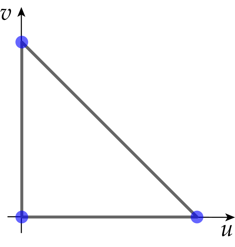
(a) First-order nodes.

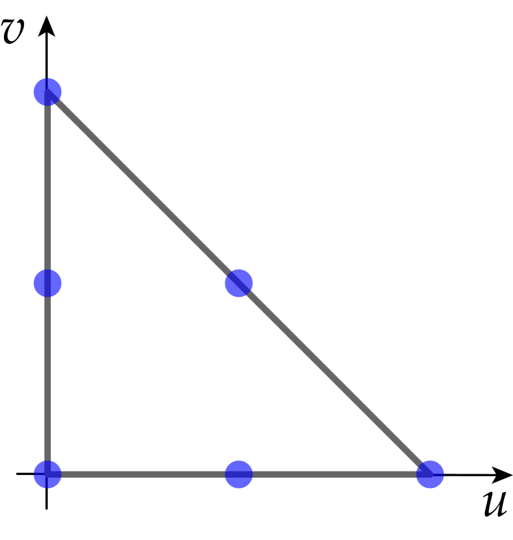
(b) Second-order nodes.

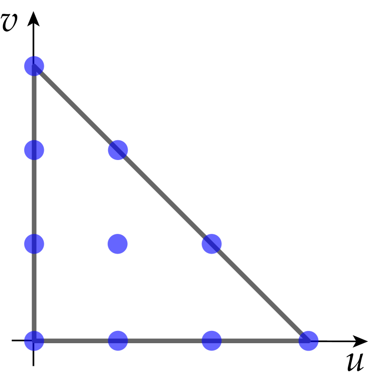
(c) Third-order nodes.

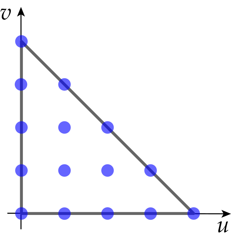
(d) Fourth-order nodes.

Figure 1: Various discretization nodes in the $uv$-plane describing curvilinear triangles

4.2   Function discretization on triangles

Not only does the surface $\Gamma$ need to be discretized, but so do any layer potential densities defined along it. Assuming each surface triangle is given as a map of the standard triangle $T_{0}$, we discretize functions along $\Gamma$ by sampling values in the $uv$-plane of each triangle $T_{j}$, i.e. $f_{j}=f_{j}(u,v)$. Sampling functions on $T_{0}$ via points in the $uv$-plane known as Vioreanu-Rokhlin nodes yields very stable interpolation formulae, as well as nearly-Gaussian quadrature schemes for bivariate polynomials [53]. Subsequent evaluation of functions at points other than the Vioreanu-Rokhlin nodes can be performed by first computing the coefficients of the corresponding Koornwinder expansion, and then evaluating this expansion at an arbitrary point $u,v$. Koornwinder polynomials can be computed using standard recurrence relations for Jacobi and Legendre polynomials [42].

4.3   Computation of layer potentials

The integral equation solvers used in the subsequent numerical examples section directly construct the matrices which apply layer potentials one at a time using either generalized Gaussian quadrature or adaptive integration, depending on whether or not the interaction is singular or not. The individual discretized layer potentials are combined to form the overall system matrix $\bm{\mathsf{A}}$, which (unless otherwise noted) is a discretization of the integral operator

$$\mathcal{A}=-\frac{I}{4}-2\mathcal{S}H\mathcal{S}^{\prime}-S\left(\mathcal{S}^{\prime\prime}+\mathcal{D}^{\prime}\right)+\mathcal{D}^{2}+\mathcal{S}\mathcal{W}\mathcal{S}.$$ (4.7)

Our solver is based on the one described in [10]. We discretize $\mathcal{S}$, $\mathcal{D}$, $\mathcal{S}^{\prime}$, and $\mathcal{S}^{\prime\prime}+\mathcal{D}^{\prime}$ in this manner. While some numerical loss of precision in evaluating the kernel of $\mathcal{S}^{\prime\prime}+\mathcal{D}^{\prime}$ occurs, it does not dominate the accuracy of the overall calculation. This procedure scales as $\mathcal{O}(N^{2})$, where $N$ denotes the number of discretization nodes of the unknown along $\Gamma$. Depending on $N$, the resulting linear system is solved via LAPACK’s $\bm{\mathsf{LU}}$ factorization [1] at a cost of $\mathcal{O}(N^{3})$, or via GMRES at a cost of $\mathcal{O}(N^{2})$.

To this end, we describe the discretization procedure in the case of the single-layer potential due to a density $\sigma$ located along the surface $\Gamma$. The discretization procedure for other layer potentials is nearly identical, with only the kernel changing. Since $\Gamma$ is described by a sequence of $n_{\text{tri}}$ curvilinear triangles $T_{j}$, we can rewrite this integral as:

$$\mathcal{S}\sigma(\bm{x}) =\int_{\Gamma}G(\bm{x}-\bm{x}^{\prime})\,\sigma(\bm{x}^{\prime})\,da(\bm{x}^{\prime})$$ (4.8)

$$=\sum_{j=1}^{n_{\text{tri}}}\int_{T_{j}}G(\bm{x}-\bm{x}^{\prime})\,\sigma(\bm{x}^{\prime})\,da(\bm{x}^{\prime})$$

$$=\sum_{j=1}^{n_{\text{tri}}}\int_{0}^{1}\int_{0}^{1-v}\frac{\sigma(\bm{x}^{j}(u,v))}{4\pi|\bm{x}-\bm{x}^{j}(u,v)|}\,\sqrt{|g(u,v)|}\,du\,dv,$$

where, as in (4.1), $\bm{x}^{j}$ is the map from the standard triangle $T_{0}$ to $T_{j}$ along $\Gamma$.

For a particular triangle $T_{j}$, if $\bm{x}\in T_{j}$, then specialized quadratures for weakly-singular kernels must be used to evaluate the integral

$$\mathcal{S}_{T_{j}}\sigma(\bm{x})=\int_{T_{j}}G(\bm{x}-\bm{x}^{\prime})\,\sigma(\bm{x}^{\prime})\,da(\bm{x}^{\prime}).$$ (4.9)

For targets $\bm{x}\notin T_{j}$, the integrand in the above expression is smooth, and can be evaluated using adaptive quadrature in parameter space, $T_{0}$.

In practice, if two surface triangles are far enough apart, the smooth Vioreanu-Rokhlin quadrature can be used instead of adaptive integration. This discretization scheme is more amenable to acceleration via fast multipole methods, but we do not discuss the procedure here as our solver implements the above scheme.

4.3.1   Singular interactions

To compute the weakly-singular integrals present in the evaluation of layer potentials, for example, computing $\mathcal{S}_{T}\sigma(\bm{x}_{i})$ when $\bm{x}_{i}$ is a discretization node located on triangle $T$, we use generalized Gaussian quadratures designed by Bremer and Gimbutas [10]. In short, after a precomputation of quadrature nodes and weights $u_{ij},v_{ij},w_{ij}$ on the standard triangle $T_{0}$ (which depend on the particular target location $u_{i},v_{i}$), the self-interaction integrals are computed as:

$$\mathcal{S}_{T}\sigma(\bm{x}_{i}) =\iint_{T}G(\bm{x}_{i},\bm{x}^{\prime})\,\sigma(\bm{x}^{\prime})\,da(\bm{x}^{\prime})$$ (4.10)

$$=\iint_{T_{0}}G(\bm{x}_{i},\bm{x}^{\prime}(u,v))\,\sigma(u,v)\,\sqrt{|g(u,v)|}\,du\,dv$$

$$\approx\sum_{j=1}^{n_{\text{quad}}}w_{ij}\,G(\bm{x}_{i},\bm{x}^{\prime}(u_{j},v_{j}))\,\sigma(u_{j},v_{j})\,\sqrt{|g(u_{j},v_{j})|}.$$

In general, the quadrature nodes do not coincide with the nodes at which $\sigma$ has been sampled. Therefore, $\sigma$ must be interpolated to each of the quadrature nodes. We then have that

$$\mathcal{S}_{T}\sigma(\bm{x}_{i})=\sum_{j=1}^{n_{\text{quad}}}w_{ij}\,G(\bm{x}_{i},\bm{x}^{\prime}(u_{j},v_{j}))\,\sqrt{|g(u_{j},v_{j})|}\sum_{k=1}^{n_{\text{pol}}}{\mathsf{V}}(j,k)\,\sigma_{k},$$ (4.11)

where $\bm{\mathsf{V}}$ denotes the matrix interpolating from the Vioreanu-Rokhlin nodes $u_{k},v_{k}$ to the quadrature nodes $u_{ij},v_{ij}$. Using the above expression, entries in the system matrix can be directly computed. See [10, 12, 11] for more information regarding the construction of similar quadratures.

4.3.2   Nearly-singular interactions

For integrals with nearly-singular kernels, i.e. those integrals (4.8) with the point $\bm{x}$ near to the triangle $T$ (usually located on an adjacent triangle), adaptive integration is performed in order to accurately construct the system matrix. In particular, given the Vioreanu-Rokhlin interpolation nodes on triangle $T$ (equivalently in parameter-space, on $T_{0}$), the density $\sigma$ can be expressed as:

$$\sigma(u,v)=\sum_{m+n\leq p}c_{mn}\,K_{mn}(u,v).$$ (4.12)

The coefficients $c_{mn}$ can be computed using the point values of $\sigma$ at the interpolation nodes $u_{j},v_{j}$ and the values of $K_{mn}$ at these same nodes. Restricting the domain of integration to a single curvilinear triangle $T$, inserting this expansion into integral (4.8), we have

$$\mathcal{S}_{T}\sigma(\bm{x}) =\iint_{T}G(\bm{x},\bm{x}^{\prime})\,\sigma(\bm{x}^{\prime})\,da(\bm{x}^{\prime})$$ (4.13)

$$=\iint_{T_{0}}G(\bm{x},\bm{x}^{\prime}(u,v))\,\sum_{m,n}c_{mn}\,K_{mn}(u,v)\,\sqrt{|g(u,v)|}\,du\,dv$$

$$=\sum_{m,n}c_{mn}\iint_{T_{0}}G(\bm{x},\bm{x}^{\prime}(u,v))\,K_{mn}(u,v)\,\sqrt{|g(u,v)|}\,du\,dv.$$

If the matrix mapping point values of $\sigma$ to coefficients in (4.12) is denoted by $\bm{\mathsf{U}}$, then each $c_{\ell}$ is given by

$$c_{\ell}=\sum_{k=1}^{n_{\text{pol}}}{\mathsf{U}}(\ell,k)\,\sigma_{k},$$ (4.14)

where $n_{\text{pol}}$ denotes the number of Koornwinder polynomials of degree $\leq p$, and the $c_{mn}$’s have been linearly ordered. In fact, $n_{\text{pol}}=(p+1)(p+2)/2$. Inserting this expression into (4.13) yields

$$\mathcal{S}_{T}\sigma(\bm{x}) =\sum_{\ell=1}^{n_{\text{pol}}}\sum_{k=1}^{n_{\text{pol}}}{\mathsf{U}}(\ell,k)\,\sigma_{k}\iint_{T_{0}}G(\bm{x},\bm{x}^{\prime}(u,v))\,K_{\ell}(u,v)\,\sqrt{|g(u,v)|}\,du\,dv$$ (4.15)

$$=\sum_{k=1}^{n_{\text{pol}}}\sigma_{k}\sum_{\ell=1}^{n_{\text{pol}}}{\mathsf{U}}(\ell,k)\,\mathcal{S}_{T}K_{\ell}(\bm{x}).$$

For each target $\bm{x}_{i}$ near to triangle $T$, the values $\mathcal{S}_{T}K_{\ell}(\bm{x}_{i})$ can be computed via adaptive integration on $T_{0}$ and summed across column elements of $\bm{\mathsf{U}}$ to compute the contribution of the point value $\sigma_{k}$ to the evaluation of $\mathcal{S}_{T}\sigma(\bm{x}_{i})$. Entries in the discretized system matrix $\bm{\mathsf{S}}$ of $\mathcal{S}$ are then given by

$${\mathsf{S}}(i,j)=\sum_{\ell=1}^{n_{\text{pol}}}{\mathsf{U}}(\ell,j)\,\mathcal{S}_{T}K_{\ell}(\bm{x}_{i}).$$ (4.16)

This procedure is then repeated for all targets not contained on $T$.

5   Numerical examples

In this section we provide several numerical experiments demonstrating the integral equation methods for solving the Laplace-Beltrami equation. Each of the following numerical examples was implemented in Fortran 90, compiled with the Intel Fortran compiler (using the MKL libraries), and executed on a 60-core machine with 4 Intel Xeon processors with 1.5Tb of shared RAM. When possible, OpenMP parallelization was used (dense matrix-vector multiplies, matrix generation, etc.).

5.1   Convergence on the sphere

In this first numerical experiment, we solve $\Delta_{\Gamma}\varphi=f$ on the unit sphere. The numerical result is compared to the exact calculation when $f$ is a spherical harmonic, whose solution is known analytically [52].

We define the spherical harmonic of degree $\ell$ and order $m$ to be $Y^{m}_{\ell}$, $|m|\leq\ell$, given by

$$Y^{m}_{\ell}(\theta,\varphi)=P^{m}_{\ell}(\cos\theta)\,e^{im\varphi}.$$ (5.1)

We have implicitly normalized the associated Legendre function $P^{m}_{\ell}$ so that

$$\int_{0}^{2\pi}\int_{0}^{\pi}\left|Y^{m}_{\ell}(\theta,\varphi)\right|^{2}\,\sin\theta\,d\theta\,d\varphi=1.$$ (5.2)

The functions $Y^{m}_{\ell}$ are orthonormal, and are the eigenfunctions of the Laplace-Beltrami operator on the sphere with eigenvalues $\lambda^{m}_{\ell}=-\ell(\ell+1)$. Using this fact, we can construct an explicit, exact solution to the Laplace-Beltrami problem

$$\Delta_{\Gamma}\varphi=Y^{m}_{\ell}.$$ (5.3)

The solution $\varphi$ is given analytically as $\varphi=-Y^{m}_{\ell}/\ell(\ell+1)$. We verify our numerical solver by reformulating problem (5.3) in integral form as before:

$$\mathcal{S}\left(\Delta_{\Gamma}+\mathcal{W}\right)\mathcal{S}\sigma=\mathcal{S}Y^{m}_{\ell}.$$ (5.4)

The right-hand side, $\mathcal{S}Y^{m}_{\ell}$ is computed numerically, and the integral equation for $\sigma$ is discretized and solved using Gaussian elimination. The solution $\varphi$ is then computed numerically as $\varphi=\mathcal{S}\sigma$ and compared with the exact solution.

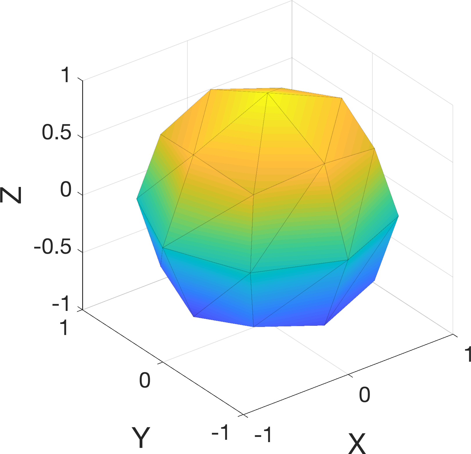
(a) $n_{\text{tri}}=48$.

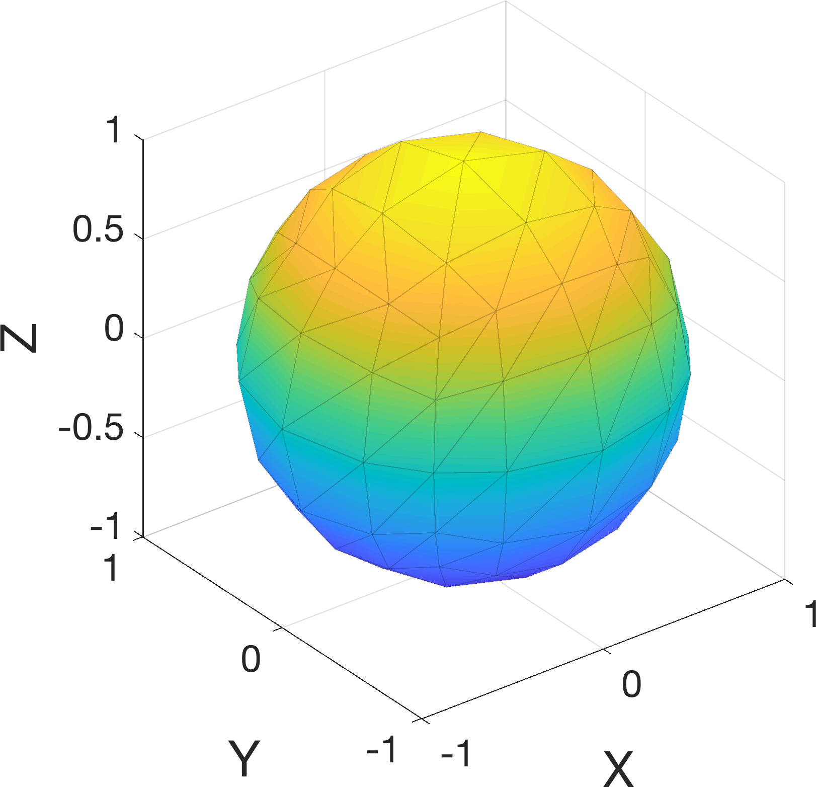
(b) $n_{\text{tri}}=192$.

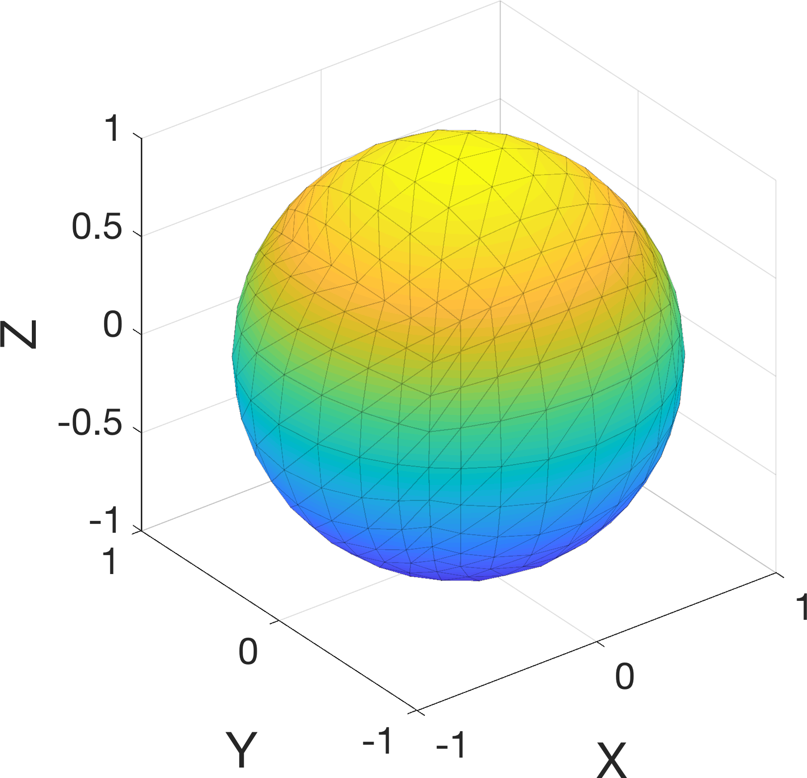
(c) $n_{\text{tri}}=768$.

Figure 2: A spherical triangulation computed by projecting an isotropic triangulation of the surface of a cube. Note that only flat projections of curvilinear triangles are plotted, analytic formulae are used to evaluate at interior points of each triangle.

A triangulation of the sphere was computed by projecting an isotropic triangulation of the surface of a cube onto the surface of the sphere; see Figure 2 for a depiction of this. Interpolation along the surface and subsequent derivatives can therefore be computed exactly in order to study the behavior of the integral equations, and not be limited by the order of discretization of the surface. Non-self interactions were computed using adaptive quadrature with an absolute tolerance of at least $10^{-10}$. Convergence results in $L^{2}$ along the sphere are given in Table 1. The column labeled $p$ denotes the order of discretization of $\sigma$ on each triangle, and $n_{\text{pts}}$ denotes the total number of discretization points: $n_{\text{pts}}=n_{\text{tri}}(p+1)(p+2)/2$. A numerical approximation to the continuous $L^{2}$ norm of the error is given by

$$||\varphi-\varphi_{\text{exact}}||_{\Gamma}^{2} =\int_{\Gamma}|\varphi-\varphi_{\text{exact}}|^{2}\,da$$ (5.5)

$$\approx\sum_{j=1}^{n_{\text{pts}}}w_{j}\,\left|\varphi_{j}+\frac{Y_{\ell}^{m}(\bm{s}_{j})}{\ell(\ell+1)}\right|^{2},$$

where $\bm{s}_{j}$ denotes the $j$th discretization node on the sphere and $w_{j}$ the corresponding $j$th smooth quadrature weight at location $\bm{s}_{j}$. The mean of the solution $\varphi$ was calculated similarly as

$$\text{mean of }\varphi =\int_{\Gamma}\varphi\,da$$ (5.6)

$$\approx\sum_{j=1}^{n_{\text{pts}}}w_{j}\,\varphi_{j}.$$

Examining these results, we see that high-order convergence is obtained in $\varphi$ on the sphere, appropriate with the order of discretization. Since the geometry information is available exactly, with $p=4$ the overall convergence order should be 4th order and with $p=8$ the overall convergence order should be 8th order. This high-order convergence is only made possible by the high-digit accuracy of the generalized Gaussian quadrature used for computing the weakly-singular integrals and the use of an exact, analytically parameterized boundary. Furthermore, the condition number of the discretization system in most cases was $\leq 10$, therefore not many digits were lost to numerical round-off when performing Gaussian elimination.

Table 1: Convergence on the sphere of the Laplace-Beltrami integral equation.

(a) Convergence for $\Delta_{\Gamma}\varphi=Y^{1}_{1}$.

$p$	$n_{\text{tri}}$	$n_{\text{pts}}$	$L^{2}$ error	mean of $\varphi$
4	48	720	$9.0\cdot 10^{-6}$	$3.3\cdot 10^{-16}$
4	192	2880	$1.4\cdot 10^{-7}$	$5.9\cdot 10^{-16}$
4	768	11520	$1.6\cdot 10^{-9}$	$1.2\cdot 16^{-15}$

(b) Convergence for $\Delta_{\Gamma}\varphi=Y^{1}_{1}$.

$p$	$n_{\text{tri}}$	$n_{\text{pts}}$	$L^{2}$ error	mean of $\varphi$
8	48	2160	$2.4\cdot 10^{-8}$	$-6.4\cdot 10^{-16}$
8	192	8640	$4.7\cdot 10^{-11}$	$-2.3\cdot 10^{-17}$
8	768	34560	$5.8\cdot 10^{-14}$	$-9.6\cdot 10^{-16}$

(c) Convergence for $\Delta_{\Gamma}\varphi=Y^{6}_{7}$.

$p$	$n_{\text{tri}}$	$n_{\text{pts}}$	$L^{2}$ error	mean of $\varphi$
4	48	720	$3.1\cdot 10^{-4}$	$-6.2\cdot 10^{-8}$
4	192	2880	$8.4\cdot 10^{-6}$	$-1.5\cdot 10^{-9}$
4	768	11520	$1.2\cdot 10^{-7}$	$-4.7\cdot 10^{-12}$

(d) Convergence for $\Delta_{\Gamma}\varphi=Y^{6}_{7}$.

$p$	$n_{\text{tri}}$	$n_{\text{pts}}$	$L^{2}$ error	mean of $\varphi$
8	48	2160	$2.3\cdot 10^{-6}$	$7.2\cdot 10^{-10}$
8	192	8640	$8.1\cdot 10^{-9}$	$2.3\cdot 10^{-14}$
8	768	34560	$1.0\cdot 10^{-11}$	$-2.0\cdot 10^{-16}$

5.2   Laplace-Beltrami on general surfaces

Except along a handful of geometries, exact solutions to the Laplace-Beltrami equation are not known. Therefore, in order to test the numerical integral equation solver we have constructed, a right-hand side must be numerically generated for which we know the solution a priori. This can be accomplished by using the relationship between the surface Laplacian and the volume Laplacian, given in Lemma 2.1.

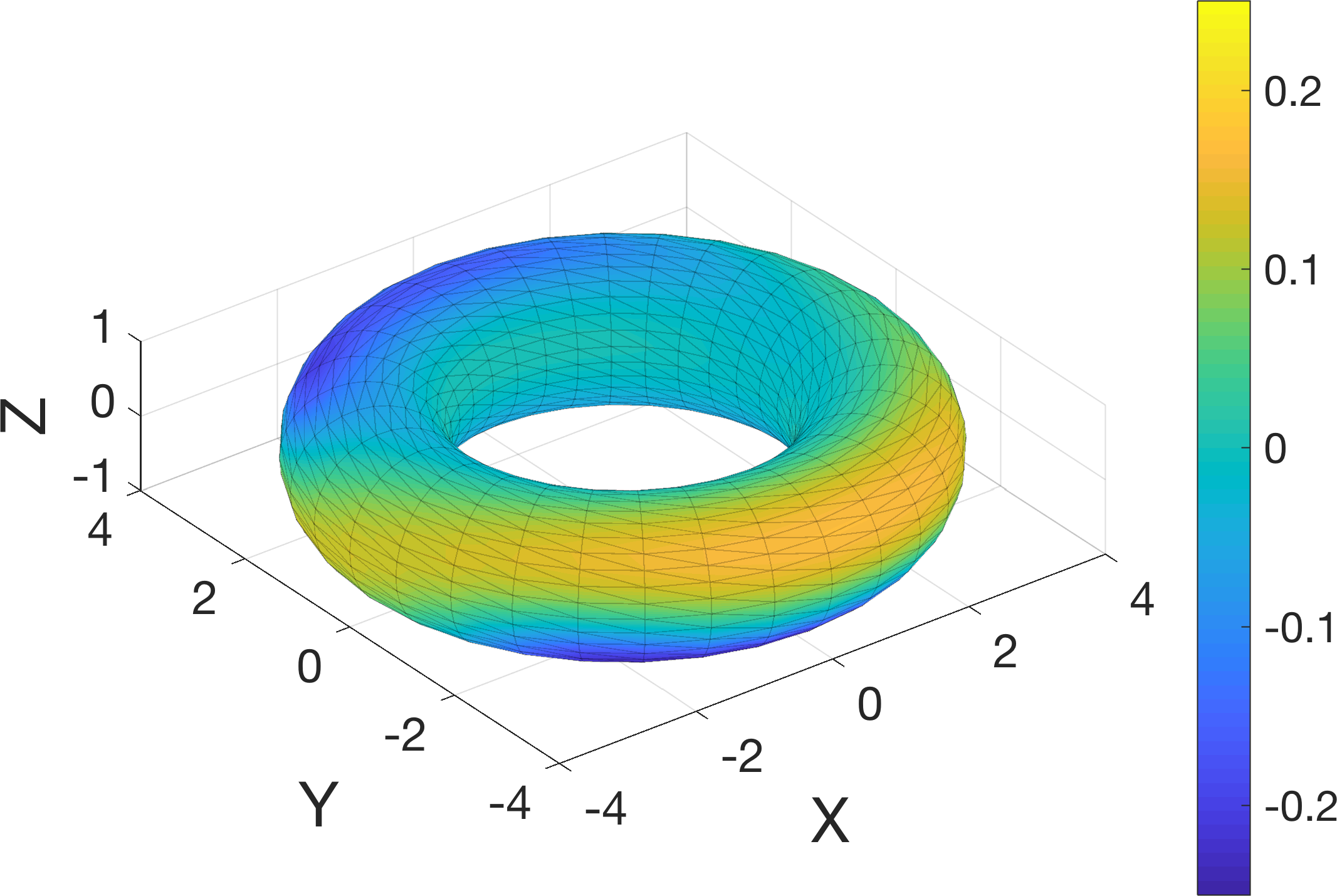
(a) The right-hand side of $\Delta_{\Gamma}\varphi=f$.

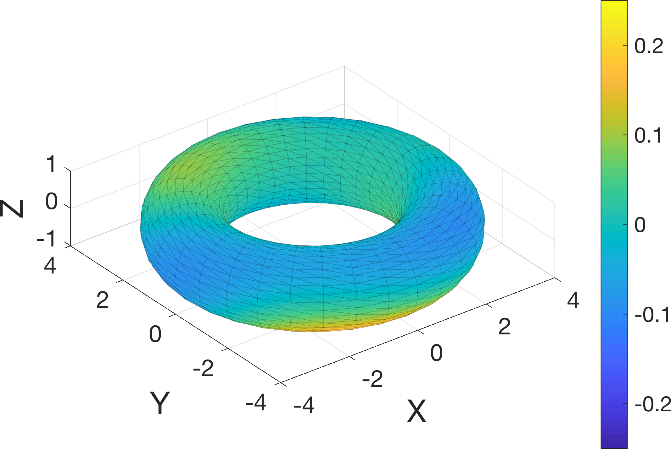
(b) The solution of $\Delta_{\Gamma}\varphi=f$.

Figure 3: The right-hand side and solution to $\Delta_{\Gamma}\varphi=f$ along the surface of a torus.

Table 2: Convergence for $\Delta_{\Gamma}\varphi=f$ along the torus using an 8th-order discretization. The condition number of the discretized matrices for $n_{\text{tri}}=32$ and $n_{\text{tri}}=128$ was was $1.8\cdot 10^{1}$. The cost of computing the SVD (and therefore the condition number) was prohibitive for $n_{\text{tri}}=512$, but a similar estimate is expected due to the stability of second-kind integral equations under refinement [2, 4].

$n_{\text{tri}}$	$n_{\text{pts}}$	$L^{2}$ error	mean of $\varphi$
32	1440	$1.6\cdot 10^{-4}$	$8.2\cdot 10^{-5}$
128	5760	$4.7\cdot 10^{-7}$	$-3.3\cdot 10^{-8}$
512	23040	$1.1\cdot 10^{-9}$	$2.1\cdot 10^{-11}$

In particular, let $g=g(x_{1},x_{2},x_{3})$ be a smooth function defined in the interior of the region bounded by $\Gamma$ and in an exterior neighborhood of $\Gamma$. Next, define the function $f$ along $\Gamma$ to be

$$f =\Delta_{\Gamma}\,g\big{|}_{\Gamma}$$ (5.7)

$$=\Delta g-2H\frac{\partial g}{\partial n}-\frac{\partial^{2}g}{\partial n^{2}}.$$

Since $f=\nabla_{\Gamma}\cdot\nabla_{\Gamma}g$, it is easy to show that $f$ has mean-zero by using Gauss’s Theorem along $\Gamma$. Then, the exact solution to the Laplace-Beltrami problem $\Delta_{\Gamma}\varphi=f$ is given by

$$\varphi=g\big{|}_{\Gamma}-\frac{1}{|\Gamma|}\int_{\Gamma}g\,da,$$ (5.8)

which is to say, the projection of $g$ onto mean-zero functions on $\Gamma$.

We first use this approach to test the surface Laplacian solver along a 3-to-1 torus, analytically parameterized as

$$x_{1}(u,v) =(3+\cos u)\cos v$$ (5.9)

$$x_{2}(u,v) =(3+\cos u)\sin v$$

$$x_{3}(u,v) =\sin u,$$

for $(u,v)\in[0,2\pi]\times[0,2\pi]$. We define the function $g$ to be

$$g(\bm{x})=C\sum_{j=1}^{10}\frac{1}{4\pi|\bm{x}-\bm{x}_{j}|},$$ (5.10)

where the $\bm{x}_{j}$ are placed randomly at a distance of 7 from the origin and $C$ is numerically calculated so that $\int_{\Gamma}|f|^{2}da=1$. The right-hand side, $f=\Delta_{\Gamma}g\big{|}_{\Gamma}$ is shown in Figure 3(a) and the solution is shown in Figure 3(b). Table 2 contains convergence results for an 8th-order discretization of the integral equation. The linear system was solved using GMRES with a relative $\ell^{2}$-residual tolerance of $10^{-14}$.

Finally, we apply our solver to geometries constructed via Computer Aided Design (CAD) software. The geometries in Figures 4 and 5 were designed in Autodesk Fusion 360 [5], exported as .step files, and then meshed using 4th-order curvilinear triangles in Gmsh [27] (whose nodal locations are given in Figure 1(d)). Take note that the right-hand sides shown in Figures 4(a) and 5(a) are not smooth. This is because of normal and curvature discontinuities generated in either the modeling or meshing procedure. Sufficient smoothing and optimization would have to be done in order to avoid this phenomenon.

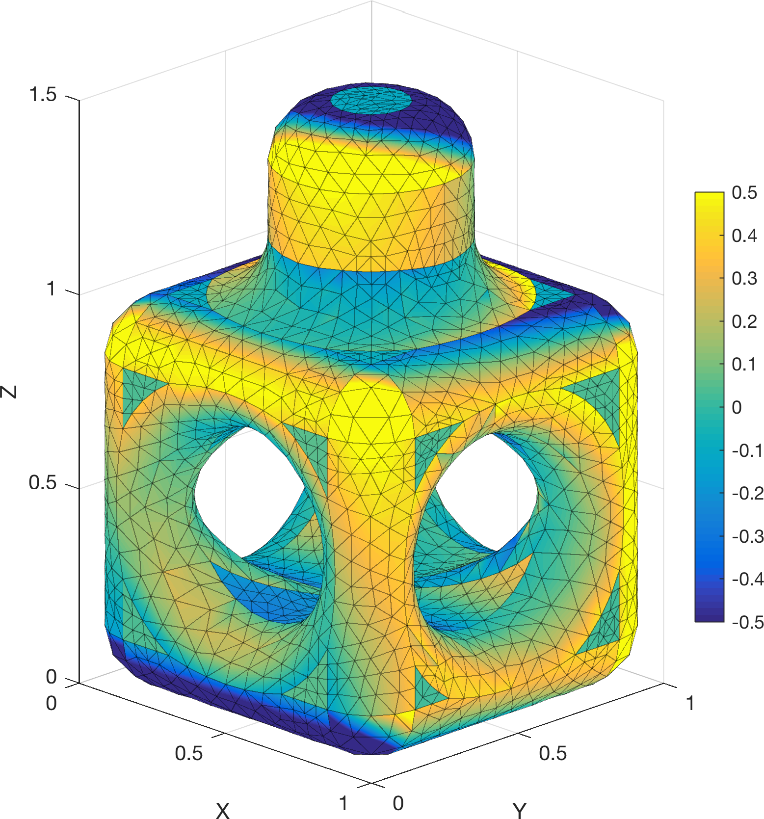
(a) The right-hand side of $\Delta_{\Gamma}\varphi=f$.

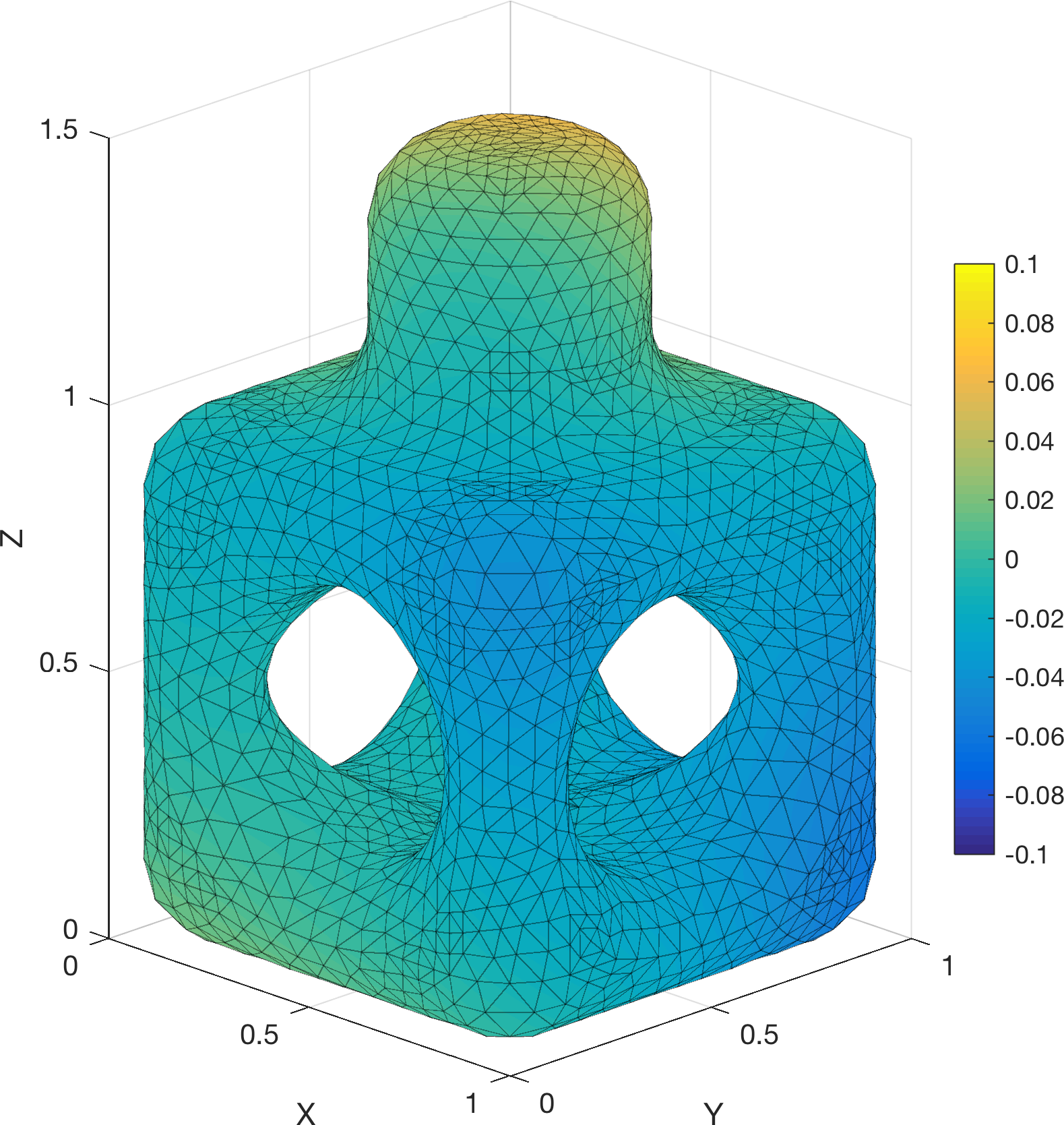
(b) The solution of $\Delta_{\Gamma}\varphi=f$.

Figure 4: The right-hand side and solution to $\Delta_{\Gamma}\varphi=f$ along a 4th-order triangulated surface. The surface consisted of 1412 triangles, was discretized using 8th-order interpolation points, resulting in 63,640 total discretization nodes. The solve resulted in an $L^{2}$ error of $2.7\cdot 10^{-2}$. The mean of the solution was $-6.8\cdot 10^{-2}$. The solve required 22 GMRES iterations and achieved a relative residual of $8.9\cdot 10^{-15}$. Note the different color scale between the images.

5.3   The Hodge decomposition

As mentioned in the introduction, any tangential vector field along smooth closed multiply connected surfaces admits what is known as a Hodge decomposition:

$$\bm{F}=\nabla_{\Gamma}\alpha+\bm{n}\times\nabla_{\Gamma}\beta+\bm{H}.$$ (5.11)

Correspondingly, given a smooth vector field $\bm{F}$, we can decompose it into its Hodge components by solving the following Laplace-Beltrami equations and computing $\bm{H}$:

$$\begin{gathered}\Delta_{\Gamma}\alpha=\nabla_{\Gamma}\cdot\bm{F},\qquad\Delta_{\Gamma}\beta=-\nabla_{\Gamma}\cdot(\bm{n}\times\bm{F}),\\ \bm{H}=\bm{F}-\nabla_{\Gamma}\alpha-\bm{n}\times\nabla_{\Gamma}\beta.\end{gathered}$$ (5.12)

To this end, we first define a smooth, arbitrary vector field $\bm{V}$ in $\mathbb{R}^{3}$ and compute $\bm{F}$ as its tangential projection onto the surface $\Gamma$: $\bm{F}=-\bm{n}\times\bm{n}\times\bm{V}$. The surface divergence of $\bm{F}$ can then be calculated in terms of the divergence of the volume vector field $\bm{V}$ as [41]:

$$\nabla_{\Gamma}\cdot\bm{F}=\nabla\cdot\bm{V}-2H\left(\bm{n}\cdot\bm{V}\right)-\frac{\partial}{\partial n}\left(\bm{n}\cdot\bm{V}\right).$$ (5.13)

In particular, we compute $\bm{V}=\bm{B}$ using the Biot-Savart Law [32] for a point current $\bm{L}$ located at $\bm{x}^{\prime}$:

$$\bm{B}(\bm{x})=\frac{\bm{L}\times(\bm{x}-\bm{x}^{\prime})}{|\bm{x}-\bm{x}^{\prime}|^{3}}.$$ (5.14)

In general, the tangential projection of $\bm{B}$ of this type will have non-zero projections onto all three components in the Hodge decomposition. The right-hand sides of the Laplace-Beltrami problems in (5.12) are automatically mean-zero, as they are exact differentials.

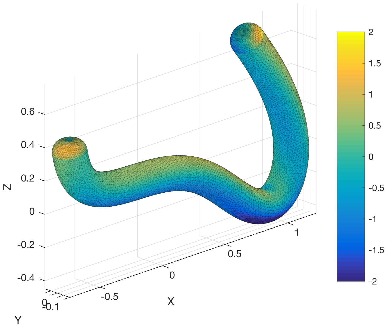
(a) The right-hand side of $\Delta_{\Gamma}\varphi=f$.

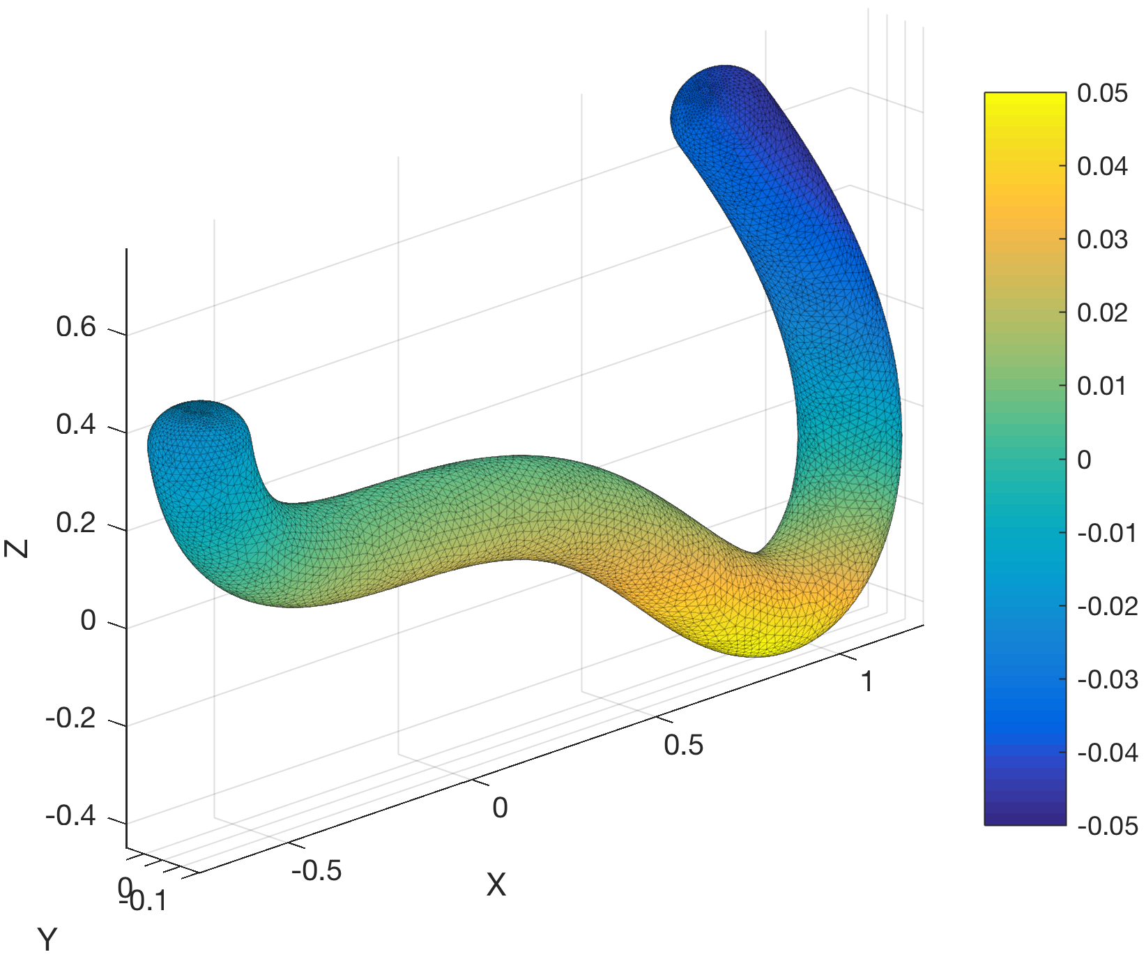
(b) The solution of $\Delta_{\Gamma}\varphi=f$.

Figure 5: The right-hand side and solution to $\Delta_{\Gamma}\varphi=f$ along a 4th-order triangulated surface. The surface consisted of 4604 triangles, was discretized using 4th-order interpolation points, resulting in 69,060 total discretization nodes. The solve resulted in an $L^{2}$ error of $1.3\cdot 10^{-3}$. The mean of the solution was $-6.7\cdot 10^{-4}$. The solve required 18 GMRES iterations and achieved a relative residual of $1.6\cdot 10^{-15}$. Note the different color scale between the images.

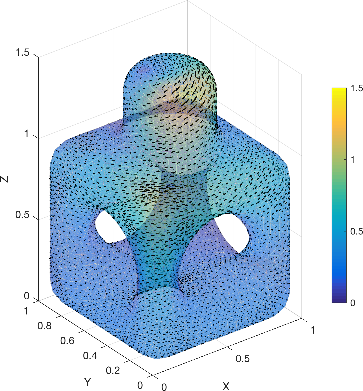
(a) The tangential projection of $\bm{B}$ onto the surface.

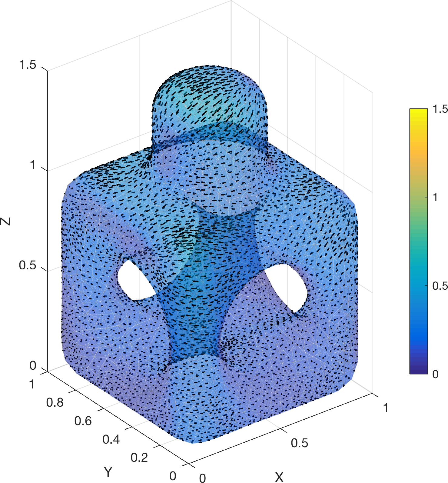
(b) The curl-free component, $\nabla_{\Gamma}\alpha$.

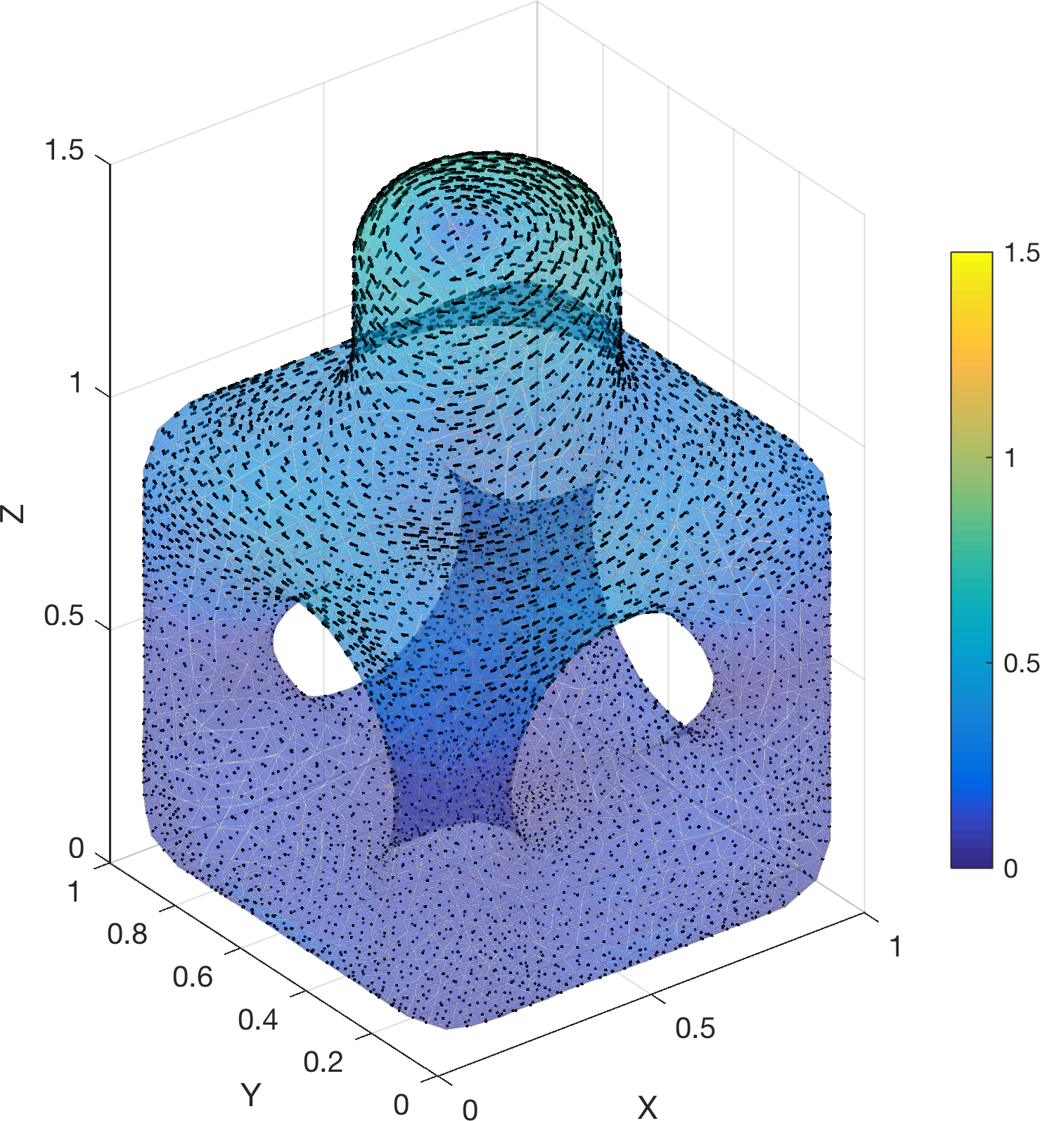
(c) The divergence-free component, $\bm{n}\times\nabla_{\Gamma}\beta$.

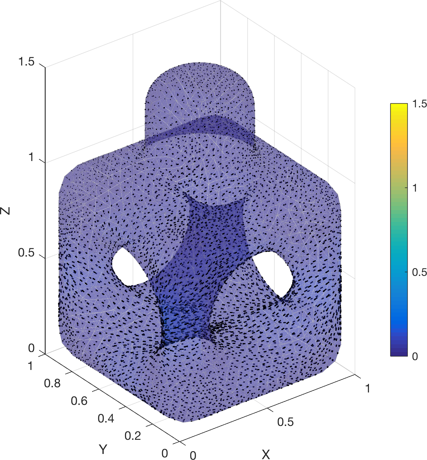
(d) The harmonic component, $\bm{H}$.

Figure 7: The Hodge decomposition of the magnetic field computed using the Biot-Savart Law due to a current element located at (0.1, 0.2, 2.1) oriented in the direction (0.37, 0.48, -0.80). The strength was computed such that $||\bm{n}\times\bm{B}||_{\Gamma}=1$. Shown is the direction and magnitude of the vector fields. The geometry is given as 4th-order curvilinear triangles, as meshed by Gmsh from a .step file created in Autodesk Fusion 360. The density was discretized using 8th-order interpolation points on 1412 triangles, yielding 63,540 discretization nodes. The linear systems were solved using GMRES and achieved relative residuals of less than $10^{-14}$. Using spectral differentiation on each triangle, $||\nabla_{\Gamma}\cdot\bm{H}||_{\Gamma}=8.9\cdot 10^{-2}$ and $||\nabla_{\Gamma}\cdot\bm{n}\times\bm{H}||_{\Gamma}=5.0\cdot 10^{-1}$. Due to the conditioning of spectral differentiation and discontinuous curvature data from the meshing procedure, these convergence results are in-line with those in Figure 4.

Once again, we use a direct version of the solver describe in [10]. Self-interactions on triangular patches are computed using the quadrature rules contained in the same work, and non-self interactions are computed using adaptive quadrature with a requested absolute tolerance of $10^{-10}$. Figure 6 shows the decomposition along the torus given by parameterization (5.9). Figure 7 shows the same decomposition along an arbitrary geometry constructed in Autodesk Fusion 360, and meshed using Gmsh. Discretization information and convergence results are provided in the captions of each figure. The $L^{2}$-norm $||\cdot||_{\Gamma}$ of a vector field along $\Gamma$ is computed as:

$$||\bm{F}||^{2}_{\Gamma} =\int_{\Gamma}|\bm{F}|^{2}\,da$$ (5.15)

$$\approx\sum_{j=1}^{n_{\text{pts}}}w_{j}\,\bm{F}^{*}_{j}\cdot\bm{F}_{j}.$$

As a proxy for convergence, since analytic Hodge decompositions are not known except on trivial geometries, we use the $L^{2}$ norm of the divergence and curl of the computed harmonic component, $\bm{H}$. Given point-wise values of $\bm{H}$ along $\Gamma$, denoted by $\bm{H}_{j}$, it is simple to compute $H^{u}_{j}$ and $H^{v}_{j}$, the coefficients with respect to the local basis:

$$\bm{H}_{j}=H^{u}_{j}\,\bm{x}_{u}+H^{v}_{j}\,\bm{x}_{v}.$$ (5.16)

The surface divergence is then given by

$$\nabla_{\Gamma}\cdot\bm{H}=\frac{1}{\sqrt{|g|}}\left(\frac{\partial}{\partial u}\left(\sqrt{|g|}H^{u}\right)+\frac{\partial}{\partial v}\left(\sqrt{|g|}H^{v}\right)\right).$$ (5.17)

Using the values $H^{u}_{j}$ and $H^{v}_{j}$ on each triangle, it is possible to form the per-triangle interpolants

$$\sqrt{|g|}\,H^{u}(u,v)=\sum_{m+n\leq p}a_{mn}\,K_{mn}(u,v),\qquad\sqrt{|g|}\,H^{v}(u,v)=\sum_{m+n\leq p}b_{mn}\,K_{mn}(u,v).$$ (5.18)

Spectral differentiation can then be used to compute the partial derivatives with respect to $u$ and $v$, and thereby enabling the computation of $\nabla_{\Gamma}\cdot\bm{H}$ (and of course, $\nabla_{\Gamma}\cdot\bm{n}\times\bm{H}$) point by point.

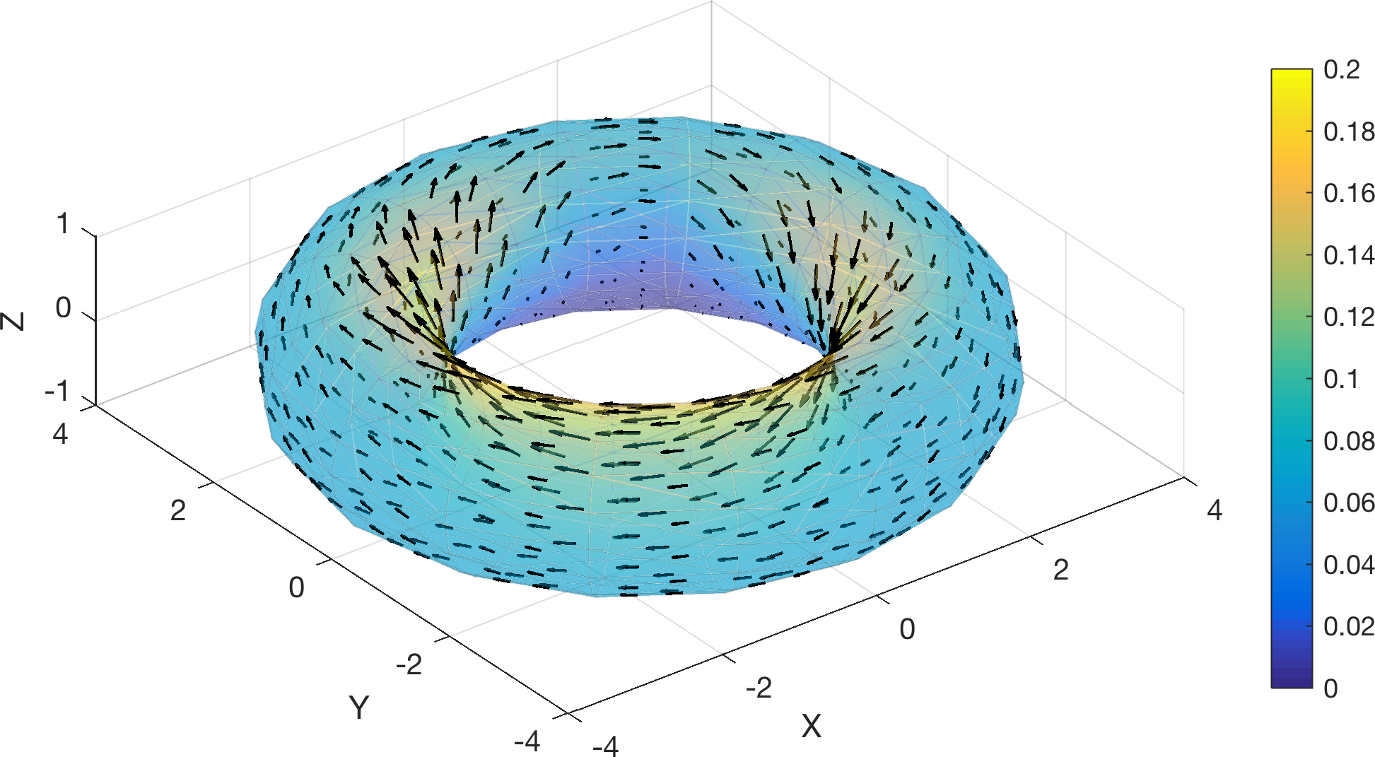
(a) The tangential projection of $\bm{B}$ onto the surface.

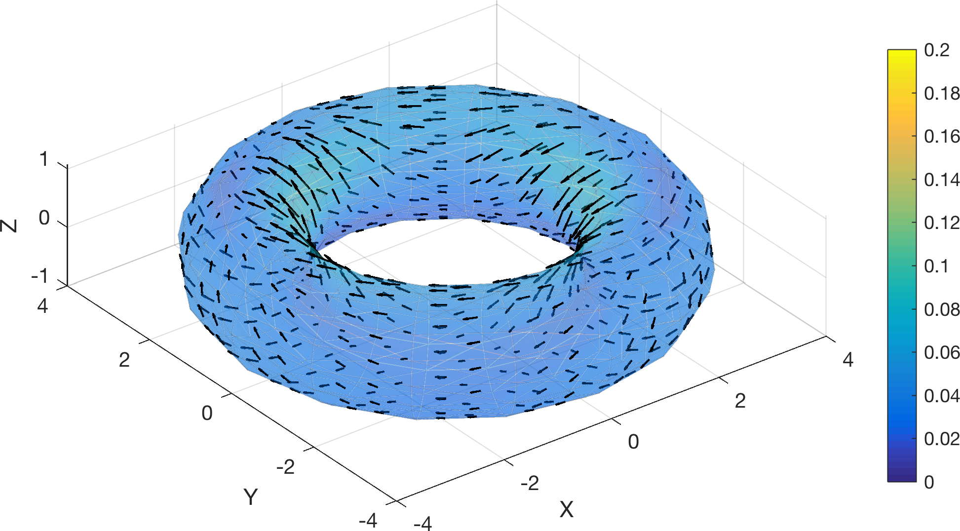
(b) The curl-free component, $\nabla_{\Gamma}\alpha$.

(c) The divergence-free component, $\bm{n}\times\nabla_{\Gamma}\beta$.

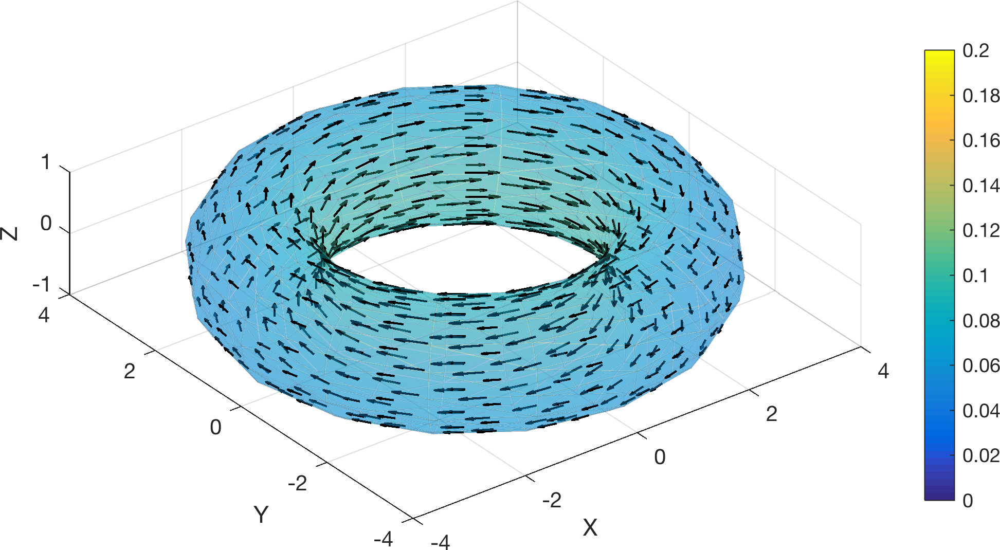
(d) The harmonic component, $\bm{H}$.

Figure 6: The Hodge decomposition of the magnetic field computed using the Biot-Savart Law due to a current element located at (0.1, 0.2, 2.1) oriented in the direction (0.37, 0.48, -0.80). The strength was computed such that $||\bm{n}\times\bm{B}||_{\Gamma}=1$. Shown is the direction and magnitude of the vector fields. The analytic parameterization of the torus was discretized using 8th-order interpolation points on 128 triangles, yielding 5760 discretization nodes. The linear systems were solved using GMRES and achieved relative residuals of less than $10^{-14}$. Using spectral differentiation on each triangle, $||\nabla_{\Gamma}\cdot\bm{H}||_{\Gamma}=5.9\cdot 10^{-5}$ and $||\nabla_{\Gamma}\cdot\bm{n}\times\bm{H}||_{\Gamma}=4.2\cdot 10^{-5}$.

6   Conclusions and future directions

In this work we have presented integral equations of the second-kind which allow for the efficient solution to the Laplace-Beltrami problem on arbitrary surfaces embedded in three dimensions. The integral equations are a consequence of left- and right-preconditioners and Calderón identities. A direct numerical solver was constructed to demonstrate the usefulness of these integral equations, and high-order accuracy was achieved for geometries which were analytically parameterized. The numerical accuracy along lower-order triangulations seems to be limited by inaccurate normal and curvature information, which is a consequence of the CAD modeling or meshing procedures. Obtaining more accurate surfaces, as well as annealing non-smooth ones, is ongoing work.

It is worth addressing the somewhat erratic convergence behavior in Tables 1 and 2. The error in any boundary integral equation method along surfaces comes from the following sources: geometry approximation, singular quadrature, nearly-singular/smooth quadrature, and the order of discretization of the unknown. The overall convergence order is dictated by the lowest order component of these factors. The discretization scheme upon which this solver was based is that presented in [10]. The convergence results in that work are similarly erratic, and provided for a 12th order scheme (see Table 2 in that work). In theory, the scheme of this paper (and of [10]) can be made to be of arbitrarily high-order (assuming access to high-order geometries is provided). The erratic convergence behavior can only be attributed to the interplay between order of convergence and actual accuracy obtained. For higher-order methods, it is often the case that the overall accuracy saturates before the asymptotic convergence rate can be observed.

It should also be noted, that while the operator $\mathcal{S}\Delta_{\Gamma}\mathcal{S}$ is equivalent to a second-kind integral operator given by

$$\mathcal{S}\Delta_{\Gamma}\mathcal{S}=-\frac{\mathcal{I}}{4}+\mathcal{D}^{2}-\mathcal{S}(\mathcal{S}^{\prime\prime}+\mathcal{D}^{\prime})-2\mathcal{S}H\mathcal{S}^{\prime},$$ (6.1)

as shown in Lemma 3.1, it may be more computationally efficient to iterate on the left-hand side operator composition $\mathcal{S}\nabla_{\Gamma}\cdot(\nabla_{\Gamma}\mathcal{S})$ instead of computing each of the three compositions on the right-hand side separately. Note that each term on the right-hand side involves normal derivatives of layer potentials, and each kernel is weakly singular. However, operators such as $\mathcal{S}\nabla_{\Gamma}\cdot$ and $\nabla_{\Gamma}\mathcal{S}$ are of order zero and have kernels which are similar to Hilbert transforms along the surface. As a consequence, a different set of singular quadratures than those used for the weakly singular kernels are required. These quadratures were, in fact, computed in [11] but were not incorporated into the solver of this paper. Exploring this iterative formulation is ongoing work, as well as efficiently coupling these integral operators and curvilinear triangulations with fast multipole methods for Laplace potentials in three dimensions.

It is relatively straightforward to develop similar integral formulations for other surface PDEs whose extensions to the volume have known Green’s functions, such as the Yukawa-Beltrami equation [37]. For example, if $\mathcal{S}_{k}$ denotes the single layer potential operator for the Helmholtz equation, then

$$\mathcal{S}_{k}\left(\Delta_{\Gamma}+k^{2}\right)\mathcal{S}_{k} =-2\mathcal{S}_{k}H\mathcal{S}_{k}^{\prime}-\mathcal{S}_{k}\mathcal{S}_{k}^{\prime\prime}$$ (6.2)

$$=-2\mathcal{S}_{k}H\mathcal{S}_{k}^{\prime}-\mathcal{S}_{k}\left(\mathcal{S}_{k}^{\prime\prime}+\mathcal{D}^{\prime}\right)+\mathcal{S}_{k}\mathcal{D}^{\prime}$$

$$=-2\mathcal{S}_{k}H\mathcal{S}_{k}^{\prime}-\mathcal{S}_{k}\left(\mathcal{S}_{k}^{\prime\prime}+\mathcal{D}^{\prime}\right)+\left(\mathcal{S}_{k}-\mathcal{S}\right)\mathcal{D}^{\prime}+\mathcal{S}\mathcal{D}^{\prime}$$

$$=-\frac{1}{4}\mathcal{I}+-2\mathcal{S}_{k}H\mathcal{S}_{k}^{\prime}-\mathcal{S}_{k}\left(\mathcal{S}_{k}^{\prime\prime}+\mathcal{D}^{\prime}\right)+\left(\mathcal{S}_{k}-\mathcal{S}\right)\mathcal{D}^{\prime}+\mathcal{D}^{2}.$$

The difference operators above for the mixed potentials can be shown to be compact, resulting in a Fredholm integral equation of the second kind. Furthermore, combining the methods of this paper with the boundary integral methods of [37, 36] would likely result in the ability to solve piece-wise constant-coefficient related Beltrami problems on surfaces.

Acknowledgements

The author would like to thank Jim Bremer and Zydrunas Gimbutas for sharing generalized Gaussian quadrature routines, and Charles L. Epstein, Leslie Greengard, Lise-Marie Imbert-Gérard, and Tonatiuh Sanchez-Vizuet for several useful discussions.

References

- [1] E. Anderson, Z. Bai, C. Bischof, S. Blackford, J. Demmel, J. Dongarra, J. Du Croz, A. Greenbaum, S. Hammarling, A. McKenney, and D. Sorensen. LAPACK Users’ Guide. Society for Industrial and Applied Mathematics, Philadelphia, PA, third edition, 1999.
- [2] P. M. Anselone. Collectively Comact Operator Approximation Theory and Applications to Integral Equations. Prentice-Hall, Englewood Cliffs, New Jersey, 1971.
- [3] T. Askham and A. J. Cerfon. An adaptive fast multipole accelerated Poisson solver for complex geometries. J. Comput. Phys., 344:1–22, 2017.
- [4] K. E. Atkinson. The Numerical Solution of Integral Equations of the Second Kind. Cambridge University Press, New York, NY, 1997.
- [5] Autodesk. Fusion 360. http://www.autodesk.com/products/fusion-360, 2017.
- [6] M. Belkin, P. Niyogi, and V. Sindhwani. Manifold Regularization: A Geometric Framework for Learning from Labeled and Unlabeled Examples. J. Mach. Learn. Res., 7:2399–2434, 2006.
- [7] M. Bertalmío, L.-T. Cheng, S. Osher, and G. Sapiro. Variational Problems and Partial Differential Equations on Implicit Surfaces. J. Comput. Phys., 174:759–780, 2001.
- [8] A. Bonito, J. M. Cascón, P. Morin, and R. H. Nochetto. AFEM for Geometric PDE: The Laplace-Beltrami Operator, pages 257–306. Springer Milan, Milano, 2013.
- [9] Y. Boubendir and C. Turc. Well-conditioned boundary integral equation formulations for the solution of high-frequency electromagnetic scattering problems. Comput. Math. Appl., 67:1772–1805, 2014.
- [10] J. Bremer and Z. Gimbutas. A Nyström method for weakly singular integral operators on surfaces. J. Comput. Phys., 231:4885–4903, 2012.
- [11] J. Bremer and Z. Gimbutas. On the numerical evaluation of singular integrals of scattering theory. J. Comput. Phys., 251:327–343, 2013.
- [12] J. Bremer, Z. Gimbutas, and V. Rokhlin. A nonlinear optimization procedure for generalized Gaussian quadratures. SIAM J. Sci. Comput., 32(4):1761–1788, 2010.
- [13] M. P. D. Carmo. Differential Geometry of Curves and Surfaces. Prentice-Hall, Englewood Cliffs, NJ, 1976.
- [14] I. Chao, U. Pinkall, P. Sanan, and P. Schröder. A Simple Geometric Model for Elastic Deformations. ACM Trans. Graph., 29, 2010.
- [15] Y. Chen and C. B. Macdonald. The Closest Point Method and Multigrid Solvers for Elliptic Equations on Surfaces. SIAM J. Sci. Comput., 37:A134–A155, 2015.
- [16] D. Colton and R. Kress. Integral Equation Methods in Scattering Theory. John Wiley & Sons, Inc., 1983.
- [17] H. Contopanagos, B. Dembart, M. Epton, J. J. Ottusch, V. Rokhlin, J. L. Visher, and S. M. Wandzura. Well-conditioned boundary integral equations for three-dimensional electromagnetic scattering. IEEE Trans. Antennas Propag., 50(12):1824–1830, 2002.
- [18] Q. I. Dai, W. C. Chew, L. J. Jiang, and Y. Wu. Differential-Forms-Motivated Discretizations of Electromagnetic Differential and Integral Equations. IEEE Ant. Wire. Propag. Lett., 13:1223–1226, 2014.
- [19] A. Demlow and G. Dziuk. An Adaptive Finite Element Method for the Laplace-Beltrami Operator on Implicitly Defined Surfaces. SIAM J. Numer. Anal., 45:421–442, 2007.
- [20] G. Dziuk and C. M. Elliott. Finite element methods for surface PDEs. Acta Numerica, 22:289–396, 2013.
- [21] C. L. Epstein and L. Greengard. Debye sources and the numerical solution of the time harmonic Maxwell equations. Commun. Pure Appl. Math., 63(4):413–463, 2010.
- [22] C. L. Epstein, L. Greengard, and M. O’Neil. Debye sources and the numerical solution of the time harmonic Maxwell equations II. Commun. Pure. Appl. Math., 66(5):753–789, 2013.
- [23] C. L. Epstein, L. Greengard, and M. O’Neil. Debye Sources, Beltrami Fields, and a Complex Structure on Maxwell Fields. Commun. Pure. Appl. Math., 68:2237–2280, 2015.
- [24] G. B. Folland. Introduction to Partial Differential Equations. Princeton University Press, Princeon, NJ, 1995.
- [25] T. Frankel. The Geometry of Physics. Cambridge University Press, New York, NY, 2011.
- [26] M. Frittelli and I. Sgura. Virtual Element Method for the Laplace-Beltrami equation on surfaces. 2016. arXiv:1612.02369 [math.NA].
- [27] C. Geuzaine and J.-F. Remacle. Gmsh: A 3-D finite element mesh generator with built-in pre- and post-processing facilities. Int. J. Num. Methods Engrg., 79:1309–1331, 2009.
- [28] L. Greengard and V. Rokhlin. A new version of the Fast Multipole Method for the Laplace equation in three dimensions. Acta Numerica, 6:229–269, 1997.
- [29] J. B. Greer, A. L. Bertozzi, and G. Sapiro. Fourth order partial differential equations on general geometries. J. Comput. Phys., 216:216–246, 2006.
- [30] P. Hansbo, M.-G. Larson, and K. Larsson. Analysis of finite element methods for vector laplacians on surfaces. 2016. arXiv:1610.06747 [math.NA].
- [31] L.-M. Imbert-Gerard and L. Greengard. Pseudo-Spectral Methods for the Laplace-Beltrami equation and the Hodge decomposition on Surfaces of Genus One. Numer. Methods Partial. Differ. Equ., 33(3):941–955, 2017.
- [32] J. D. Jackson. Classical Electrodynamics. Wiley, New York, NY, 3rd edition, 1999.
- [33] T. Koornwinder. Two-variable analogues of the classical orthogonal polynomials. In Theory and application of special functions (Proc. Advanced Sem., Math. Res. Center, Univ. Wisconsin, Madison, Wis., 1975), pages 435–495. Academic Press New York, 1975.
- [34] R. Kress. Linear Integral Equations. Springer, New York, NY, 2014.
- [35] R. Kress and G. Roach. Transmission problems for the Helmholtz equation. J. Math. Phys., 19:1433–1437, 1978.
- [36] M. C. A. Kropinski and N. Nigam. Fast integral equation methods for the Laplace-Beltrami equation on the sphere. Adv. Comput. Math., 40(2):577–596, 2014.
- [37] M. C. A. Kropinski, N. Nigam, and B. Quaife. Integral equation methods for the Yukawa-Beltrami equation on the sphere. Advances in Computational Mathematics, 42(2):469–488, 2016.
- [38] C. B. Macdonald and S. J. Ruuth. Level Set Equations on Surfaces via the Closest Point Method. J. Sci. Comput., 35:219–240, 2008.
- [39] C. B. Macdonald and S. J. Ruuth. The Implicit Closest Point Method for the Numerical Solution of Partial Differential Equations on Surfaces. SIAM J. Sci. Comput., 31:4330–4350, 2009.
- [40] H. P. McKean and I. M. Singer. Curvature and the eigenvalues of the Laplacian. J. Diff. Geom., 1:43–69, 1967.
- [41] J.-C. Nedelec. Acoustic and Electromagnetic Equations. Springer, New York, NY, 2001.
- [42] F. W. Olver, D. W. Lozier, R. F. Boisvert, and C. W. Clark. NIST Handbook of Mathematical Functions. Cambridge University Press, New York, NY, USA, 1st edition, 2010.
- [43] C. H. Papas. Theory of Electromagnetic Wave Propagation. Dover, New York, NY, 1988.
- [44] M. Reuter. Hierarchical Shape Segmentation and Registration via Topological Features of Laplace-Beltrami Eigenfunctions. Int. J. Comput. Vision, 89:287–308, 2010.
- [45] V. Rokhlin. Solution of acoustic scattering problems by means of second kind integral equations. Wave Motion, 5:257–272, 1983.
- [46] S. J. Ruuth and B. Merriman. A simple embedding method for solving partial differential equations on surfaces. J. Comput. Phys., 227:1943–1961, 2008.
- [47] Y. Saad and M. H. Schultz. GMRES: A Generalized Minimal Residual Algorithm for Solving Nonsymmetric Linear Systems. SIAM J. Sci. Stat. Comput., 7:856–869, 1986.
- [48] P. Schwartz, D. Adalsteinsson, P. Colella, A. P. Arkin, and M. Onsum. Numerical computation of diffusion on a surface. Proc. Nat. Acad. Sci., 102:11151–11156, 2005.
- [49] J. Sifuentes, Z. Gimbutas, and L. Greengard. Randomized methods for rank-deficient linear systems. Elec. Trans. Num. Anal., 44:177–188, 2015.
- [50] J. Sokolowski and J.-P. Zolesio. Introduction to Shape Optimization. Springer, New York, NY, 1992.
- [51] S. K. Veerapaneni, A. Rahimian, G. Biros, and D. Zorin. A fast algorithm for simulating vesicle flows in three dimensions. J. Comput. Phys., 230:5610–5634, 2011.
- [52] F. Vico, L. Greengard, and Z. Gimbutas. Boundary integral equation analysis on the sphere. Numer. Math., 128:463–487, 2014.
- [53] B. Vioreanu and V. Rokhlin. Spectra of Multiplication Operators as a Numerical Tool. SIAM J. Sci. Comput., 36:A267–A288, 2014.
- [54] Y. Weiss, A. Torralba, and R. Fergus. Spectral hashing. In Advances in neural information processing systems, pages 1753–1760, 2009.