A lowest-order composite finite element exact sequence on pyramids

Abstract.

Composite basis functions for pyramidal elements on the spaces $H^{1}(\Omega)$, $H(\mathrm{curl},\Omega)$, $H(\mathrm{div},\Omega)$ and $L^{2}(\Omega)$ are presented. In particular, we construct the lowest-order composite pyramidal elements and show that they respect the de Rham diagram, i.e. we have an exact sequence and satisfy the commuting property. Moreover, the finite elements are fully compatible with the standard finite elements for the lowest-order Raviart-Thomas-Nédélec sequence on tetrahedral and hexahedral elements. That is to say, the new elements have the same degrees of freedom on the shared interface with the neighbouring hexahedral or tetrahedra elements, and the basis functions are conforming in the sense that they maintain the required level of continuity (full, tangential component, normal component, …) across the interface. Furthermore, we study the approximation properties of the spaces as an initial partition consisting of tetrahedra, hexahedra and pyramid elements is successively subdivided and show that the spaces result in the same (optimal) order of approximation in terms of the mesh size $h$ as one would obtain using purely hexahedral or purely tetrahedral partitions.

1. Introduction

A key issue in performing finite element analysis in complex three dimensional applications is the meshing of the domain $\Omega$. Given a choice, many practitioners would opt for a mesh consisting entirely of brick, or hexahedral elements. Unfortunately, meshing complicated domains using only hexahedral elements is far from straightforward. By way of contrast, current mesh generators based on tetrahedral elements are readily available and are routinely used to mesh even quite complicated domains in three dimensions.

The relative efficiency with which hexahedral elements can be used to fill space compared with tetrahedral elements has led to an increasing use [3, 29] of tetrahedral-hexadral-pyramidal (THP) partitions in which hexahedral elements are used on part of the domain whereas tetrahedral elements are used in sub-domains where the use of hexahedral elements would pose difficulties. Pyramidal elements are used to interface between hexahedral and tetrahedral elements.

At first glance, THP partitions would seem to provide the best of both worlds—at least as far as the issue of meshing goes. Difficulties arise when one turns to the question of choosing the basis functions for the pyramidal elements. Here, we have in mind applications including: primal formulations of elasticity, requiring elements in the space $H^{1}(\Omega)$ for which full interelement continuity is needed; electromagnetics, requiring vector-valued elements in the space $H(\mathrm{curl},\Omega)$ for which only the continuity of tangential components is needed; mixed formulations of porous media flow, using vector-valued elements in the space $H(\mathrm{div},\Omega)$ for which only continuity of normal components is needed, along with scalar valued elements in the space $L^{2}(\Omega)$.

The choice of degrees of freedom and the types of basis function that can be used in the pyramidal elements is constrained by the requirement for the resulting elements to be compatible with neighbouring hexahedral and tetrahedral finite elements. Indeed, the need for compatibility between hexahedra-pyramids and between tetrahedra-pyramids dictates the choice of the degree of freedom on the pyramid. The problems start when one seeks to select a basis for the pyramidal elements.

Firstly, the basis functions for the hexadral and tetrahedral elements are polynomial on the interfaces. This dictates that the basis functions on the faces of the pyramids must be polynomials of exactly the same type as those on the neighbouring element. This would be fine were it not for the fact that it is impossible to achieve this using polynomial basis functions on the pyramidal elements. While it is quite possible to proceed by using rational basis functions on the pyramids [4, 19, 32, 33, 34, 26, 27, 5, 7, 6, 8, 17, 12, 13, 18, 15], this path gives rise to a new set of issues relating to computations involving the rational functions and their approximation properties.

Secondly, the pyramidal basis functions used to discretise the spaces $H^{1}(\Omega)$, $H(\mathrm{curl},\Omega)$, $H(\mathrm{div},\Omega)$ and $L^{2}(\Omega)$ should not be chosen in isolation. For instance, if finite element discretisation of mixed formulations are to be stable and consistent then it is necessary for the finite element spaces to be exact and for the associated de Rham diagram to commute. These terms will be defined more precisely later but for now it suffices to realise that there are additional constraints beyond that of simply maintaining compatibility with hexahedral and tetrahedral elements.

An alternative approach avoiding the need for rational basis functions, and one that is perhaps rather more akin to the spirit of the finite element method itself, consists of using a composite or macro element basis for the pyramidal elements. In other words, the basis functions on the individual pyramids are, by analogy with the finite element method, constructed using piecewise polynomials on a subdivision of the pyramid. A natural choice consists of subdividing the pyramid into a pair of tetrahedra [35, 21, 9, 23, 22, 1]. Of course, the use of composite element poses its own challenges.

In the present work we explore the use of composite basis functions for pyramidal elements on the spaces $H^{1}(\Omega)$, $H(\mathrm{curl},\Omega)$, $H(\mathrm{div},\Omega)$ and $L^{2}(\Omega)$. In particular, we construct the lowest-order composite pyramidal elements and show that they respect the de Rham diagram, i.e. we have an exact sequence and satisfy the commuting property. Moreover, the finite elements are fully compatible with the standard finite elements for the lowest-order Raviart-Thomas-Nédélec sequence [25, 2] on tetrahedral and hexahedral elements. That is to say, the new elements have the same degrees of freedom on the shared interface with the neighbouring hexahedral or tetrahedra elements, and the basis functions are conforming in the sense that they maintain the required level of continuity (full, tangential component, normal component, …) across the interface. Furthermore, we study the approximation properties of the spaces as an initial THP partition is successively subdivided and show that the spaces result in the same (optimal) order of approximation in terms of the mesh size $h$ as one would obtain using purely hexahedral or purely tetrahedral partitions. In short, all of the properties one would wish to have of lowest-order pyramidal elements are shown to hold along with the added bonus that composite elements are readily handled using standard finite element technology.

The existing literature loc. cit. on composite elements is limited to $H^{1}$-conforming finite elements—our finite element and basis functions coincide with that proposed in [35] for the $H^{1}(\Omega)$ case. However, many problems of practical interest are naturally posed over a mixture of the spaces $H(\mathrm{curl})$, $H(\mathrm{div})$ or $L^{2}$ in addition to $H^{1}(\Omega)$. As such the absence of lowest-order composite $H(\mathrm{curl})$-, our $H(\mathrm{div})$-, and $L^{2}$-conforming finite elements constitutes a severe limitation for the use of finite element approximation on THP partitions. The present work fills this gap in the literature.

The remainder of this article is organized as follows. Section 2 gives a brief overview of the standard lowest-order spaces on hexahedral and tetrahedral elements with which we are seeking to maintain compatibility, and contains preliminaries on the pyramidal geometry and polynomial spaces in two dimensions. In Section 3, we introduce the lowest-order composite finite elements on a pyramid. In Section 4, we present the lowest-order global finite elements on tetrahedral-hexahedral-pyramidal (THP) partitions and prove their approximation properties on a sequence of uniformly refined (non-affine) THP partitions.

2. Review of Lowest Order Hexahedral and Tetrahedral Elements

In this section, we introduce various notations and take the opportunity to briefly review the lowest order finite elements on hexahedral and tetrahedra with which we require the new pyramidal elements to be compatible.

2.1. Lowest-order finite elements on a tetrahedron and a hexahedron

Let us first recall the lowest order finite elements on the reference tetrahedron

$$\widehat{T}=\{(x,y,z):0<x,y,z<1,x+y+z<1\},$$ (1a)

and the reference hexahedron

$$\widehat{H}=\{(x,y,z):0<x,y,z<1\}.$$ (1b)

The lowest-order $H^{1}$-conforming finite elements and the associated (vertex-based) basis functions on the reference tetrahedron and reference hexahedron are given in Table 1. Here $\mathbb{P}_{k}(\widehat{T})$ stands for the space of polynomials of total degree no greater than $k$ on the reference tetrahedron, and $\mathbb{Q}_{k}(\widehat{H})$ stands for the space of tensor-product polynomials of degree no greater than $k$ in each argument on the reference hexahedron.

element $\widehat{K}$	space $S(\widehat{K})$	$\#$	basis
$\widehat{T}$	$\mathbb{P}_{1}(\widehat{T})$	4	$\phi_{1}=1-x-y-z$,
			$\phi_{2}=x$,    $\phi_{3}=y,\;\;\phi_{4}=z,$.
$\widehat{H}$	$\mathbb{Q}_{1}(\widehat{H})$	8	$\phi_{1}=(1-x)(1-y)(1-z),$ $\phi_{2}=x(1-y)(1-z),$
			$\phi_{3}=xy(1-z),$ $\phi_{4}=(1-x)y(1-z)$,
			$\phi_{5}=(1-x)(1-y)z,$ $\phi_{6}=x(1-y)z$,
			$\phi_{7}=xyz,$ $\phi_{8}=(1-x)yz$.

Table 1. Lowest order $H^{1}$-conforming finite elements on the reference tetrahedron and reference hexahedron.

The lowest-order $H(\mathrm{curl})$-conforming finite elements and the associated (edge-based) basis functions on the reference tetrahedron and reference hexahedron are given in Table 2. Here the lowest-order Nédélec spaces of the first kind are given as follows:

$$\mathbb{ND}_{0}(\widehat{T}):= \;\mathbb{P}_{0}(\widehat{T})^{3}\oplus\boldsymbol{x}\times\mathbb{P}_{0}(\widehat{T})^{3},$$

$$\mathbb{ND}_{0}(\widehat{H}):= \;\left(\mathbb{P}_{0,1,1}(\widehat{H}),\mathbb{P}_{1,0,1}(\widehat{H}),\mathbb{P}_{1,1,0}(\widehat{H})\right)^{\sf{T}},$$

where $\mathbb{P}_{\ell,m,n}(\widehat{H})$ stands for the space of tensor-product polynomials of degree no greater than $\ell$ in the first argument, $m$ in the second argument, and $n$ in the third argument on the reference hexahedron.

element $\widehat{K}$	space $\boldsymbol{E}(\widehat{K})$	$\#$	basis
$\widehat{T}$	$\mathbb{ND}_{0}(\widehat{T})$	6	$\boldsymbol{\varphi}_{1}=x{\nabla}y-y{\nabla}x$, $\boldsymbol{\varphi}_{2}=z{\nabla}x+z{\nabla}y+(1-x-y){\nabla}z$,
			$\boldsymbol{\varphi}_{3}=y{\nabla}z-z{\nabla}y$, $\boldsymbol{\varphi}_{4}=(1-y-z){\nabla}x+x{\nabla}y+x{\nabla}z,$
			$\boldsymbol{\varphi}_{5}=z{\nabla}x-x{\nabla}z$, $\boldsymbol{\varphi}_{6}=y{\nabla}x+(1-x-z){\nabla}y+y{\nabla}z.$
$\widehat{H}$	$\mathbb{ND}_{0}(\widehat{H})$	12	$\boldsymbol{\varphi}_{1}=(1-y)(1-z){\nabla}x,\boldsymbol{\varphi}_{2}=(1-y)z{\nabla}x,\boldsymbol{\varphi}_{3}=y(1-z){\nabla}x$,
			$\boldsymbol{\varphi}_{4}=(1-z)(1-x){\nabla}y,\boldsymbol{\varphi}_{5}=(1-z)x{\nabla}y,\boldsymbol{\varphi}_{6}=z(1-x){\nabla}y$,
			$\boldsymbol{\varphi}_{7}=(1-x)(1-y){\nabla}z,\boldsymbol{\varphi}_{8}=(1-x)y{\nabla}z,\boldsymbol{\varphi}_{9}=x(1-y){\nabla}z$,
			$\boldsymbol{\varphi}_{10}=yz{\nabla}x,\boldsymbol{\varphi}_{11}=zx{\nabla}y,\boldsymbol{\varphi}_{12}=xy{\nabla}z$.

Table 2. Lowest order $H(\mathrm{curl})$-conforming finite elements on the reference tetrahedron and reference hexahedron.

The lowest-order $H(\mathrm{div})$-conforming finite elements and the associated (face-based) basis functions on the reference tetrahedron and reference hexahedron are given in Table 3. Here the lowest-order Raviart-Thomas spaces are given as follows:

$$\mathbb{RT}_{0}(\widehat{T}):= \;\mathbb{P}_{0}(\widehat{T})^{3}\oplus\boldsymbol{x}\,\mathbb{P}_{0}(\widehat{T}),$$

$$\mathbb{RT}_{0}(\widehat{H}):= \;\left(\mathbb{P}_{1,0,0}(\widehat{H}),\mathbb{P}_{0,1,0}(\widehat{H}),\mathbb{P}_{0,0,1}(\widehat{H})\right)^{\sf{T}}.$$

element $\widehat{K}$	space $\boldsymbol{V}(\widehat{K})$	$\#$	basis
$\widehat{T}$	$\mathbb{RT}_{0}(\widehat{T})$	4	$\boldsymbol{\psi}_{1}=2(x{\nabla}x+y{\nabla}y+z{\nabla}z)$,
			$\boldsymbol{\psi}_{2}=2((x-1){\nabla}x+y{\nabla}y+z{\nabla}z)$,
			$\boldsymbol{\psi}_{3}=2(x{\nabla}x+(y-1){\nabla}y+z{\nabla}z)$,
			$\boldsymbol{\psi}_{4}=2(x{\nabla}x+y{\nabla}y+(z-1){\nabla}z)$.
$\widehat{H}$	$\mathbb{RT}_{0}(\widehat{H})$	6	$\boldsymbol{\psi}_{1}=(x-1){\nabla}x,\;\;\;\boldsymbol{\psi}_{2}=x{\nabla}x,$
			$\boldsymbol{\psi}_{3}=(y-1){\nabla}y,\;\;\;\boldsymbol{\psi}_{4}=y{\nabla}y$,
			$\boldsymbol{\psi}_{5}=(z-1){\nabla}z,\;\;\;\boldsymbol{\psi}_{6}=z{\nabla}z$.

Table 3. Lowest order $H(\mathrm{div})$-conforming finite elements on the reference tetrahedron and reference hexahedron.

The lowest-order $L^{2}$-conforming finite elements and the associated (cell-based) basis functions on the reference tetrahedron and reference hexahedron are given in Table 4.

element $\widehat{K}$	space $W(\widehat{K})$	$\#$	basis
$\widehat{T}$	$\mathbb{P}_{0}(\widehat{T})$	1	$\psi_{1}=6$
$\widehat{H}$	$\mathbb{Q}_{0}(\widehat{H})$	1	$\psi_{1}=1$

Table 4. Lowest order $L^{2}$-conforming finite elements on the reference tetrahedron and reference hexahedron.

Let $\Phi_{K}:\widehat{K}\rightarrow K$ be a continuously differentiable, invertible and surjective map. If $\widehat{\boldsymbol{x}}$ denotes a coordinate system on the reference element $\widehat{K}$, then $\boldsymbol{x}=\Phi_{K}(\widehat{\boldsymbol{x}})$ is the corresponding coordinate system on the physical element $K$. The Jacobian matrix of the mapping $\Phi_{K}$ with respect to the reference coordinates and its determinant are denoted by

$$F_{K}(\widehat{{\boldsymbol{x}}})=\left(\frac{\partial\Phi_{K,i}}{\partial\hat{x}_{j}}(\widehat{{\boldsymbol{x}}})\right)_{1\leq i,j\leq 3},\quad J_{K}(\widehat{{\boldsymbol{x}}})=\det(F_{K}(\widehat{{\boldsymbol{x}}})).$$

Finite elements on a physical element $K$ are defined in terms of a reference element $\widehat{K}$ via mapping in the usual way [24]:

$$S(K):= \;\{v\in H^{1}(K):\; \;\;v=\widehat{v}\circ\Phi_{K}^{-1},\quad \forall\;\widehat{v}\in S(\widehat{K})\},$$ (2a)

$${\boldsymbol{E}}(K):= \;\{{\boldsymbol{v}}\in H(\mathrm{curl},K):\; \;\;{\boldsymbol{v}}=F_{K}^{-T}\widehat{{\boldsymbol{v}}}\circ\Phi_{K}^{-1},\quad \forall\;\widehat{{\boldsymbol{v}}}\in{\boldsymbol{E}}(\widehat{K})\},$$ (2b)

$${\boldsymbol{V}}(K):= \;\{{\boldsymbol{v}}\in H(\mathrm{div},K):\; \;\;{\boldsymbol{v}}=J_{K}^{-1}F_{K}\widehat{{\boldsymbol{v}}}\circ\Phi_{K}^{-1},\quad \forall\;\widehat{{\boldsymbol{v}}}\in{\boldsymbol{V}}(\widehat{K})\},$$ (2c)

$$W(K):= \;\{v\in L^{2}(K):\; \;\;v=J_{K}^{-1}\widehat{v}\circ\Phi_{K}^{-1},\quad \forall\;\widehat{v}\in W(\widehat{K})\},$$ (2d)

where $\widehat{K}$ is either the reference tetrahedron $\widehat{T}$, or the reference hexahedron $\widehat{H}$, and the reference finite elements $S(\widehat{K})$, ${\boldsymbol{E}}(\widehat{K})$, ${\boldsymbol{V}}(\widehat{K})$, and $W(\widehat{K})$ are given in Table 1–4. In particular, a basis for the physical element is obtained by applying the appropriate mapping to the basis defined on the reference element.

2.2. Regular pyramid

Let us now introduce notation on the pyramidal element that will be used later on. Let $K\subset\mathbb{R}^{3}$ be a regular pyramid consisting of five vertices $\mathsf{v}_{1},\cdots,\mathsf{v}_{5}$ ordered as shown in Figure 1, where $\mathsf{v}_{1},\mathsf{v}_{2},\mathsf{v}_{3},\mathsf{v}_{4}$ form a parallelogram. The pyramid is cut into two tetrahedra, $T_{1}$ and $T_{2}$, by forming a new triangular face using the vertices $\mathsf{v}_{1}$, $\mathsf{v}_{3}$, and $\mathsf{v}_{5}$ as shown in Figure 1. The local vertex ordering of the two tetrahedra is also depicted in Figure 1.

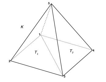
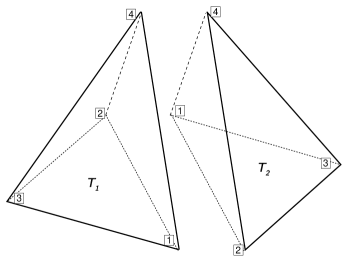
Figure 1. Left: a regular pyramid cut into two tetrahedra. Right: local vertex ordering of each tetrahedra.

The pyramid consists of five vertices

$$\mathcal{V}(K)=\{\mathsf{v}_{1},\mathsf{v}_{2},\mathsf{v}_{3},\mathsf{v}_{4},\mathsf{v}_{5}\},$$

eight edges

$$\mathcal{E}(K)=\{\mathsf{e}_{12},\;\mathsf{e}_{14},\;\mathsf{e}_{15},\;\mathsf{e}_{23},\;\mathsf{e}_{25},\;\mathsf{e}_{34},\;\mathsf{e}_{35},\;\mathsf{e}_{45}\},$$

where $\mathsf{e}_{ij}=[\mathsf{v}_{i},\mathsf{v}_{j}]$ is the edge connecting vertices $\mathsf{v}_{i}$ and $\mathsf{v}_{j}$, and five faces

$$\mathcal{F}(K)=\{\mathsf{f}_{125},\;\mathsf{f}_{145},\;\mathsf{f}_{235},\;\mathsf{f}_{345},\;\mathsf{f}_{1234}\},$$

where $\mathsf{f}_{ijk}=[\mathsf{v}_{i},\mathsf{v}_{j},\mathsf{v}_{k}]$ is a triangular face, and $\mathsf{f}_{1234}=[\mathsf{v}_{1},\mathsf{v}_{2},\mathsf{v}_{3},\mathsf{v}_{4}]$ is the base parallelogram face. Moreover, let $\mathcal{F}_{t}(K)\subset\mathcal{F}(K)$ denote the set of triangular faces of $K$, and $\mathcal{F}_{s}(K)\subset\mathcal{F}(K)$ denote the set containing the base parallelogram face of $K$.

2.3. Polynomial spaces in two dimensions

Given an element $T\subset\mathbb{R}^{2}$, we us $\mathbb{P}_{p}(T)$ to denote the space of polynomials with total degree at most $p$ defined on $T$. When $T\subset\mathbb{R}^{2}$ is the unit square, we use $\mathbb{P}_{p_{1},p_{2}}(T)$ to denote the space of tensor-product polynomials with degree at most $p_{1}$ in the $x$-coordinate, and $p_{2}$ in the $y$-coordinate. We also denote $\mathbb{Q}_{p}(T):=\mathbb{P}_{p,p}(T)$.

The lowest-order Nédélec spaces of the first kind (rotated Raviart-Thomas) on the reference triangle $\hat{\mathsf{f}}_{t}$ and reference square $\hat{\mathsf{f}}_{s}$ in $\mathbb{R}^{2}$ with Cartesian coordinates $(x,y)$ are given as follows:

$$\mathbb{ND}^{I}_{0}(\hat{\mathsf{f}}_{t}):= \;\mathbb{P}_{0}(\hat{\mathsf{f}}_{t})^{2}\oplus\boldsymbol{x}\times\mathbb{P}_{0}(\hat{\mathsf{f}}_{t}),$$

$$\mathbb{ND}^{I}_{0}(\hat{\mathsf{f}}_{s}):= \;[\mathbb{P}_{0,1}(\hat{\mathsf{f}}_{s}),\;\mathbb{P}_{1,0}(\hat{\mathsf{f}}_{s})]^{T}.$$

Here $\boldsymbol{x}\times v$ denotes the vector $[y\,v,-x\,v]^{T}$ where $v$ is a scalar-valued function. The lowest-order Nédélec space of the first kind on a physical triangle or quadrilateral in $\mathbb{R}^{3}$ is defined in terms of the corresponding space on the reference element via the standard covariant Piola mapping:

$$\mathbb{ND}^{I}_{0}({\mathsf{f}_{t}}):= \;\{(J_{t}^{\dagger})^{T}\boldsymbol{\phi}\,\circ F_{t}^{-1}:\;\;\;\boldsymbol{\phi}\in\mathbb{ND}^{I}_{0}(\hat{\mathsf{f}}_{t})\},$$ (3a)

$$\mathbb{ND}^{I}_{0}({\mathsf{f}_{s}}):= \;\{(J_{s}^{\dagger})^{T}\boldsymbol{\phi}\,\circ F_{s}^{-1}:\;\;\;\boldsymbol{\phi}\in\mathbb{ND}^{I}_{0}(\hat{\mathsf{f}}_{s}),\}$$ (3b)

where $F_{t}$ is the (affine) mapping from the reference triangle $\hat{\mathsf{f}}_{t}$ in $\mathbb{R}^{2}$ to the physical triangle $\mathsf{f}_{t}$ in $\mathbb{R}^{3}$, $J_{t}\in\mathbb{R}^{3\times 2}$ is the Jacobian matrix, and

$$J_{t}^{\dagger}=(J_{t}^{T}\,J_{t})^{-1}J_{t}^{T}$$

is the pseudo-inverse. Similarly, $F_{s}$ is the bilinear mapping from $\hat{\mathsf{f}}_{s}$ to $\mathsf{f}_{s}$, and $J_{s}\in\mathbb{R}^{3\times 2}$ is the associated Jacobian matrix.

Throughout this paper, we write $a\preceq b$, when $a\leq C\,b$ with a generic constant $C$ independent of $a,b$, and the mesh size.

3. Lowest-order composite finite elements on a pyramid

In this section, we present the lowest-order composite finite element family on a regular pyramid. These finite elements have degrees of freedom compatible with standard finite elements on tetrahedra and hexahedra. Moreover, the set functions used to define element reduce to those used for tetrahedra and hexahedra on the faces. They can be naturally combined with the standard, lowest-order, Raviart-Thomas-Nédélec finite elements to provide $H^{1}$-, $H(\mathrm{curl})$-, $H(\mathrm{div})$-, and $L^{2}$-conforming finite element spaces on a conforming hybrid mesh consisting of tetrahedra, pyramids, and hexahedra. Commuting diagrams are also respected at both element level on a single pyramid and globally on a hybrid mesh.

The classic definition of a finite element [11, 14] as a triple is recalled below for convenience:

Definition 1.

A finite element consists of a triple $(K,\mathcal{P}_{K},\Sigma_{K})$ where:

1. the element domain $K\subset\mathbb{R}^{n}$ is a bounded closed set with nonempty interior and piece-wise smooth boundary,

2. the space of shape functions $\mathcal{P}_{K}$ is a finite-dimensional space of functions on $K$,

3. the set of nodal variables $\Sigma_{K}=\{N_{1}^{K},\cdots,N_{k}^{K}\}$, or degrees of freedom, forms a basis for $\mathcal{P}_{K}^{\prime}$, where $\mathcal{P}_{K}^{\prime}$ denotes the dual space of $\mathcal{P}_{K}$.

We shall specify our spaces in terms of the nodal basis $\{\phi_{1},\phi_{2},\cdots,\phi_{k}\}$ for $\mathcal{P}_{K}$ dual to $\Sigma_{K}$ (i.e. $N_{i}(\phi_{j})=\delta_{ij}$).

To begin, recall that the regular pyramid $K$ is split into two tetrahedra $T_{1}$ and $T_{2}$ by connecting vertices $\mathsf{v}_{1}$ and $\mathsf{v}_{3}$, as shown in Figure 1. The barycentric coordinates on each tetrahedron will be used to construct our basis functions. Let $\lambda_{i}^{T_{\ell}}$ ($i=1,2,3,4,\;\ell=1,2$) denote the affine function that vanishes at all vertices of the tetrahedron $T_{\ell}$ except the $i$-th vertex, where it attains value $1$. For example, with vertices ordered as in Figure 1, $\lambda_{1}^{T_{1}}$ is the affine function, which vanishes on the face $\mathsf{f}_{125}$ and takes the value $1$ at the vertex $\mathsf{v}_{3}$.

Next, we present a new, lowest order, finite element sequence on the pyramid which we view as a composite element formed from the tetrahedra $T_{1}$ and $T_{2}$. We then show that the elements satisfy the exact sequence property and exhibit explicit interpolation operators which are shown to satisfy the commuting diagram property.

3.1. The $H^{1}$-conforming finite element

We present the lowest-order $H^{1}$-conforming composite finite element on a regular pyramid.

Definition 2.

The lowest-order composite $H^{1}$-conforming finite element is is defined by $(K,S(K),\Sigma^{S}_{K})$ where

• $K$ is a regular pyramid with parallelogram base,

• $$S(K):= \;\{v\in H^{1}(K): \;v\raise-0.86108pt\hbox{$|$}_{T_{\ell}}\in\mathbb{P}_{2}(T_{\ell}),\;\;\ell=1,2,$$ (4)

  $$\;\;\;v\raise-0.86108pt\hbox{$|$}_{\mathsf{f}}\in\mathbb{P}_{1}(\mathsf{f}),\quad\forall\mathsf{f}\in\mathcal{F}_{t}(K),$$

  $$\;\;\;v\raise-0.86108pt\hbox{$|$}_{\mathsf{f}}\in\mathbb{Q}_{1}(\mathsf{f}),\quad\forall\mathsf{f}\in\mathcal{F}_{s}(K).\}$$

• $\Sigma_{K}^{S}=\mathrm{span}\{N_{i}^{S}:\;i=1,2,3,4,5\}$ where

  $$N_{i}^{S}:=N_{i}^{\mathsf{v}}:v\longrightarrow v(\mathsf{v}_{i})\quad\forall\mathsf{v}_{i}\in\mathcal{V}_{K}.$$

  are point evaluation functionals at the vertices of $K$.

Lemma 1.

The triplet $(K,S(K),\Sigma^{S}_{K})$ is a finite element of dimension 5. The set $\{\phi^{S}_{i}:\;i=1,2,\cdots,5\}$ is the nodal basis dual to $\Sigma^{S}_{K}$, where

$$\phi_{1}^{S}= \;\left\{\begin{tabular}[]{l l}$\lambda_{2}^{T_{1}}-\lambda_{1}^{T_{1}}\lambda_{2}^{T_{1}}$&on $T_{1}$\vspace{0.2cm}\\ $\lambda_{1}^{T_{2}}-\lambda_{1}^{T_{2}}\lambda_{2}^{T_{2}}$&on $T_{2}$\end{tabular}\right.,\quad \phi_{2}^{S}=\left\{\begin{tabular}[]{l l}$\lambda_{3}^{T_{1}}+\lambda_{1}^{T_{1}}\lambda_{2}^{T_{1}}$&on $T_{1}$\vspace{0.2cm}\\ $\lambda_{1}^{T_{2}}\lambda_{2}^{T_{2}}$&on $T_{2}$\end{tabular}\right.,$$

$$\phi_{3}^{S}= \left\{\begin{tabular}[]{l l}$\lambda_{1}^{T_{1}}-\lambda_{1}^{T_{1}}\lambda_{2}^{T_{1}}$&on $T_{1}$\vspace{0.2cm}\\ $\lambda_{2}^{T_{2}}-\lambda_{1}^{T_{2}}\lambda_{2}^{T_{2}}$&on $T_{2}$\end{tabular}\right.,\quad \phi_{4}^{S}=\left\{\begin{tabular}[]{l l}$\lambda_{1}^{T_{1}}\lambda_{2}^{T_{1}}$&on $T_{1}$\vspace{0.2cm}\\ $\lambda_{3}^{T_{2}}+\lambda_{1}^{T_{2}}\lambda_{2}^{T_{2}}$&on $T_{2}$\end{tabular}\right.,$$

$$\phi_{5}^{S}= \left\{\begin{tabular}[]{l l}$\lambda_{4}^{T_{1}}$&on $T_{1}$\vspace{0.2cm}\\ $\lambda_{4}^{T_{2}}$&on $T_{2}$\end{tabular}\right.,$$

i.e., $N_{i}^{S}(\phi_{j}^{S})=\delta_{ij}.$

Proof.

First, it is easy to check that each of the above functions $\phi_{i}^{S}$ belongs to $S(K)$ and satisfies $N_{i}^{S}(\phi_{j}^{S})=\delta_{ij}$. Hence,

$$\dim S(K)\geq\dim\left(\mathrm{span}\{\phi_{i}^{S}:\;1\leq i\leq 5\}\right)=5.$$ (5)

Now, we prove unisolvence of the set of degrees of freedom $\Sigma^{S}_{K}$. Let $u\in S(K)$ be such that $N_{i}^{S}(u)=0$ for $i=1,2,\cdots,5$. In other words, $u$ vanishes at all vertices of $K$. Since the restriction of $u$ to a triangular face is a linear polynomial or to the quadrilateral face is a bilinear polynomial, we immediately have $u\raise-0.86108pt\hbox{$|$}_{\mathsf{f}}=0$ on all faces $\mathsf{f}\in\mathcal{F}(K)$. Hence, $u\raise-0.86108pt\hbox{$|$}_{T_{\ell}}\in\mathbb{P}_{2}(T_{\ell})$, for $\ell=1,2$, and $u$ vanishes on three faces of $T_{\ell}$. This implies that $u=0$. Hence, we have $\dim S(K)\leq\dim\Sigma^{S}_{K}\leq 5$. Inequality (5) now shows $\dim S(K)=5$, and the unisolvence of the set $\Sigma^{S}_{K}$ follows. ∎

3.2. The $H(\mathrm{curl})$-conforming finite element

We present the lowest-order $H(\mathrm{curl})$-conforming composite finite element on a regular pyramid. To simplify notation, we label the edges as follows:

$$\mathsf{E}_{1}=\mathsf{e}_{12},\;\mathsf{E}_{2}=\mathsf{e}_{14},\;\mathsf{E}_{3}=\mathsf{e}_{15},\;\mathsf{E}_{4}=\mathsf{e}_{23},$$

$$\mathsf{E}_{5}=\mathsf{e}_{25},\;\mathsf{E}_{6}=\mathsf{e}_{34},\;\mathsf{E}_{7}=\mathsf{e}_{35},\;\mathsf{E}_{8}=\mathsf{e}_{45},$$

and orient the edges so that the the tangential vector ${\boldsymbol{t}}_{i}$ on $\mathsf{E}_{i}$ point from the lower vertex number to higher vertex number.

Definition 3.

The lowest-order composite $H(\mathrm{curl})$-conforming finite element is is defined by $(K,{\boldsymbol{E}}(K),\Sigma^{{\boldsymbol{E}}}_{K})$ where

• $K$ is a regular pyramid with parallelogram base,

• $$\boldsymbol{E}(K):= \;\{{\boldsymbol{v}}\in H(\mathrm{curl},K): \;{\boldsymbol{v}}\raise-0.86108pt\hbox{$|$}_{T_{\ell}}\in\mathbb{P}_{1}(T_{\ell})^{3},\;\;\ell=1,2,$$ (6)

  $$\!\!\!\!\!\!\!\!\!\!\!\!\!\!\!\!\!\!{\boldsymbol{n}}\times({\boldsymbol{v}}\times{\boldsymbol{n}})\raise-0.86108pt\hbox{$|$}_{\mathsf{f}}\in\mathbb{ND}^{I}_{0}(\mathsf{f}),\quad\forall\,\mathsf{f}\in\mathcal{F}(K)\},$$

  where ${\boldsymbol{n}}$ is the unit outward normal vector on face $\mathsf{f}$.

• $\Sigma_{K}^{{\boldsymbol{E}}}=\mathrm{span}\{N_{i}^{{\boldsymbol{E}}}:\;1\leq i\leq 8\}$, where

  $$N_{i}^{{\boldsymbol{E}}}:=N_{i}^{\mathsf{E}}:{\boldsymbol{v}}\longrightarrow\int_{\mathsf{E}_{i}}{\boldsymbol{v}}\cdot{\boldsymbol{t}}_{i}\,\mathrm{ds}\quad\forall\,\mathsf{E}_{i}\in\mathcal{E}_{K}.$$

We denote the Whitney edge form on the tetrahedral $T_{\ell}$, $\ell=1,2$, as

$${\boldsymbol{\omega}}_{ij}^{T_{\ell}}:=\lambda_{i}^{T_{\ell}}{\nabla}\lambda_{j}^{T_{\ell}}-\lambda_{j}^{T_{\ell}}{\nabla}\lambda_{i}^{T_{\ell}}.$$

A basis for the space ${\boldsymbol{E}}(K)$ is given as follows.

Lemma 2.

The triplet $(K,{\boldsymbol{E}}(K),\Sigma^{{\boldsymbol{E}}}_{K})$ is a finite element of dimension 8. The set $\{{\boldsymbol{\varphi}}^{{\boldsymbol{E}}}_{i}:\;i=1,2,\cdots,8\}$ is the nodal basis dual to $\Sigma^{{\boldsymbol{E}}}_{K}$, where

$${\boldsymbol{\varphi}}^{{\boldsymbol{E}}}_{1}= \left\{\begin{tabular}[]{l l}${\boldsymbol{\omega}}_{23}^{T_{1}}+\lambda_{2}^{T_{1}}{\nabla}\lambda_{1}^{T_{1}}$&on $T_{1}$\vspace{0.2cm}\\ $\lambda_{1}^{T_{2}}{\nabla}\lambda_{2}^{T_{2}}$&on $T_{2}$\end{tabular}\right.,\quad {\boldsymbol{\varphi}}^{{\boldsymbol{E}}}_{2}=\left\{\begin{tabular}[]{l l}$\lambda_{2}^{T_{1}}{\nabla}\lambda_{1}^{T_{1}}$&on $T_{1}$\vspace{0.2cm}\\ ${\boldsymbol{\omega}}_{13}^{T_{2}}+\lambda_{1}^{T_{2}}{\nabla}\lambda_{2}^{T_{2}}$&on $T_{2}$\end{tabular}\right.,$$

$${\boldsymbol{\varphi}}^{{\boldsymbol{E}}}_{3}= \left\{\begin{tabular}[]{l l}${\boldsymbol{\omega}}_{24}^{T_{1}}$&on $T_{1}$\vspace{0.2cm}\\ ${\boldsymbol{\omega}}_{14}^{T_{2}}$&on $T_{2}$\end{tabular}\right.,\quad {\boldsymbol{\varphi}}^{{\boldsymbol{E}}}_{4}=\left\{\begin{tabular}[]{l l}${\boldsymbol{\omega}}_{31}^{T_{1}}-\lambda_{1}^{T_{1}}{\nabla}\lambda_{2}^{T_{1}}$&on $T_{1}$\vspace{0.2cm}\\ $-\lambda_{2}^{T_{2}}{\nabla}\lambda_{1}^{T_{2}}$&on $T_{2}$\end{tabular}\right.,$$

$${\boldsymbol{\varphi}}^{{\boldsymbol{E}}}_{5}= \left\{\begin{tabular}[]{l l}${\boldsymbol{\omega}}_{34}^{T_{1}}$&on $T_{1}$\vspace{0.2cm}\\ $0$&on $T_{2}$\end{tabular}\right.,\quad {\boldsymbol{\varphi}}^{{\boldsymbol{E}}}_{6}=\left\{\begin{tabular}[]{l l}$\lambda_{1}^{T_{1}}{\nabla}\lambda_{2}^{T_{1}}$&on $T_{1}$\vspace{0.2cm}\\ ${\boldsymbol{\omega}}_{23}^{T_{2}}+\lambda_{2}^{T_{2}}{\nabla}\lambda_{1}^{T_{2}}$&on $T_{2}$\end{tabular}\right.,$$

$${\boldsymbol{\varphi}}^{{\boldsymbol{E}}}_{7}= \left\{\begin{tabular}[]{l l}${\boldsymbol{\omega}}_{14}^{T_{1}}$&on $T_{1}$\vspace{0.2cm}\\ ${\boldsymbol{\omega}}_{24}^{T_{2}}$&on $T_{2}$\end{tabular}\right.,\quad {\boldsymbol{\varphi}}^{{\boldsymbol{E}}}_{8}=\left\{\begin{tabular}[]{l l}$0$&on $T_{1}$\vspace{0.2cm}\\ ${\boldsymbol{\omega}}_{34}^{T_{2}}$&on $T_{2}$\end{tabular}\right.,$$

i.e., $N_{i}^{{\boldsymbol{E}}}({\boldsymbol{\varphi}}_{j}^{{\boldsymbol{E}}})=\delta_{ij}$.

Proof.

The proof is similar to that for the $H^{1}$ case. First, we can verify directly from the definition that each function ${\boldsymbol{\varphi}}_{i}^{{\boldsymbol{E}}}$ belongs to ${\boldsymbol{E}}(K)$ and satisfies $N_{i}^{{\boldsymbol{E}}}({\boldsymbol{\varphi}}_{j}^{{\boldsymbol{E}}})=\delta_{ij}$. Hence,

$$\dim{\boldsymbol{E}}(K)\geq\dim\left(\mathrm{span}\{{\boldsymbol{\varphi}}_{i}^{{\boldsymbol{E}}}:\;1\leq i\leq 8\}\right)=8.$$

Next, we prove unisolvence of the set of degrees of freedom $\Sigma^{E}_{K}$. Let ${\boldsymbol{u}}\in{\boldsymbol{E}}(K)$ be such that $N_{i}^{{\boldsymbol{E}}}({\boldsymbol{u}})=0$ for $i=1,2,\cdots,8$. In other words, the tangential trace of ${\boldsymbol{u}}$ vanishes on all edges of $K$. Since the tangential trace of ${\boldsymbol{u}}$ on a face belongs to the lowest-order Nédélec ​​ space of the first kind, we immediately have the tangential traces of ${\boldsymbol{u}}$ vanishes on all faces of $K$. Hence, ${\boldsymbol{u}}\raise-0.86108pt\hbox{$|$}_{T_{\ell}}\in\mathbb{P}_{1}(T_{\ell})^{3}$, for $\ell=1,2$, and $u$ has vanishing tangential traces on three faces of $T_{\ell}$. This implies that ${\boldsymbol{u}}={\boldsymbol{0}}$. Hence, $\dim{\boldsymbol{E}}(K)=8$, and the set $\Sigma_{K}^{{\boldsymbol{E}}}$ is unisolvent. ∎

3.3. The $H(\mathrm{div})$-conforming finite element

We present the lowest-order $H(\mathrm{div})$-conforming composite finite element on a regular pyramid. To simplify notation, let faces be labelled such that

$$\mathsf{F}_{1}=\mathsf{f}_{125},\;\mathsf{F}_{2}=\mathsf{f}_{145},\;\mathsf{F}_{3}=\mathsf{f}_{235},\;\mathsf{F}_{4}=\mathsf{f}_{345},\;\mathsf{F}_{5}=\mathsf{f}_{1234}.$$

Definition 4.

The lowest-order composite $H(\mathrm{div})$-conforming finite element is defined by $(K,{\boldsymbol{V}}(K),\Sigma^{{\boldsymbol{V}}}_{K})$ where

• $K$ is a regular pyramid with parallelogram base,

• $$\boldsymbol{V}(K):= \;\{{\boldsymbol{v}}\in H(\mathrm{div},K): \;{\boldsymbol{v}}\raise-0.86108pt\hbox{$|$}_{T_{\ell}}\in\mathbb{P}_{0}(T_{\ell})^{3}\oplus\boldsymbol{x}\mathbb{P}_{0}(T_{\ell}),\;\;\ell=1,2,$$ (7)

  $$\;\;{\boldsymbol{v}}\cdot{\boldsymbol{n}}\raise-0.86108pt\hbox{$|$}_{\mathsf{f}}\in\mathbb{P}_{0}(\mathsf{f}),\quad\forall\mathsf{f}\in\mathcal{F}(K)\},$$

  where ${\boldsymbol{n}}$ is the unit outward normal vector on face $\mathsf{f}$.

• $\Sigma_{K}^{{\boldsymbol{V}}}=\mathrm{span}\{N_{i}^{{\boldsymbol{V}}}:\;1\leq i\leq 6\}$, where

  $$N_{i}^{{\boldsymbol{V}}}:=N_{i}^{\mathsf{F}}:{\boldsymbol{v}}\longrightarrow\int_{\mathsf{F}_{i}}{\boldsymbol{v}}\cdot{\boldsymbol{n}}\,\mathrm{ds}\quad\forall\,\mathsf{F}_{i}\in\mathcal{F}_{K},$$

  are the total normal fluxes over each face $\mathsf{F}_{i}\in\mathcal{F}_{K}$, and

  $$N_{6}^{{\boldsymbol{V}}}:=N_{0}^{\mathrm{C}}:{\boldsymbol{v}}\longrightarrow\int_{T_{1}}{\nabla\cdot}{\boldsymbol{v}}\,\mathrm{dx}-\int_{T_{2}}{\nabla\cdot}{\boldsymbol{v}}\,\mathrm{dx}.$$

  is a cell-based degrees of freedom.

We denote the Whitney face form on the tetrahedral $T_{\ell}$, $\ell=1,2$ as

$${\boldsymbol{\chi}}_{ijk}^{T_{\ell}}:=\lambda_{i}^{T_{\ell}}{\nabla}\lambda_{j}^{T_{\ell}}\times{\nabla}\lambda_{k}^{T_{\ell}}+\lambda_{j}^{T_{\ell}}{\nabla}\lambda_{k}^{T_{\ell}}\times{\nabla}\lambda_{i}^{T_{\ell}}+\lambda_{k}^{T_{\ell}}{\nabla}\lambda_{i}^{T_{\ell}}\times{\nabla}\lambda_{j}^{T_{\ell}}.$$

A basis for the space ${\boldsymbol{V}}(K)$ is given as follows.

Lemma 3.

The triplet $(K,{\boldsymbol{V}}(K),\Sigma^{{\boldsymbol{V}}}_{K})$ is a finite element of dimension 6. The set $\{{\boldsymbol{\psi}}^{{\boldsymbol{V}}}_{i}:\;i=1,2,\cdots,6\}$ is the nodal basis dual to $\Sigma^{{\boldsymbol{V}}}_{K}$, where

$${\boldsymbol{\psi}}^{{\boldsymbol{V}}}_{1}= \left\{\begin{tabular}[]{l l}$2\,{\boldsymbol{\chi}}_{234}^{T_{1}}-{\boldsymbol{\chi}}_{124}^{T_{1}}$&on $T_{1}$\vspace{0.2cm}\\ ${\boldsymbol{\chi}}_{124}^{T_{2}}$&on $T_{2}$\end{tabular}\right.,\quad {\boldsymbol{\psi}}^{{\boldsymbol{V}}}_{2}=\left\{\begin{tabular}[]{l l}${\boldsymbol{\chi}}_{124}^{T_{1}}$&on $T_{1}$\vspace{0.2cm}\\ $2\,{\boldsymbol{\chi}}_{143}^{T_{2}}-{\boldsymbol{\chi}}_{124}^{T_{2}}$&on $T_{2}$\end{tabular}\right.,$$

$${\boldsymbol{\psi}}^{{\boldsymbol{V}}}_{3}= \left\{\begin{tabular}[]{l l}$2\,{\boldsymbol{\chi}}_{143}^{T_{1}}-{\boldsymbol{\chi}}_{124}^{T_{1}}$&on $T_{1}$\vspace{0.2cm}\\ ${\boldsymbol{\chi}}_{124}^{T_{2}}$&on $T_{2}$\end{tabular}\right.,\quad {\boldsymbol{\psi}}^{{\boldsymbol{V}}}_{4}=\left\{\begin{tabular}[]{l l}${\boldsymbol{\chi}}_{124}^{T_{1}}$&on $T_{1}$\vspace{0.2cm}\\ $2\,{\boldsymbol{\chi}}_{234}^{T_{2}}-{\boldsymbol{\chi}}_{124}^{T_{2}}$&on $T_{2}$\end{tabular}\right.,$$

$${\boldsymbol{\psi}}^{{\boldsymbol{V}}}_{5}= \left\{\begin{tabular}[]{l l}${\boldsymbol{\chi}}_{132}^{T_{1}}$&on $T_{1}$\vspace{0.2cm}\\ ${\boldsymbol{\chi}}_{132}^{T_{2}}$&on $T_{2}$\end{tabular}\right.,\quad {\boldsymbol{\psi}}^{{\boldsymbol{V}}}_{6}=\left\{\begin{tabular}[]{l l}${\boldsymbol{\chi}}_{124}^{T_{1}}$&on $T_{1}$\vspace{0.2cm}\\ $-{\boldsymbol{\chi}}_{124}^{T_{2}}$&on $T_{2}$\end{tabular}\right.,$$

i.e., $N_{i}^{{\boldsymbol{V}}}({{\boldsymbol{\psi}}}^{{\boldsymbol{V}}}_{j})=\delta_{ij}$.

Proof.

The proof is again similar to the previous two cases, and is therefore omitted. ∎

3.4. The $L^{2}$-conforming finite element

We present the lowest-order $L^{2}$-conforming composite finite element on a regular pyramid.

Definition 5.

The lowest-order composite $H(\mathrm{div})$-conforming finite element is defined by $(K,{\boldsymbol{V}}(K),\Sigma^{{\boldsymbol{V}}}_{K})$ where

• $K$ is a regular pyramid with parallelogram base,

• $$W(K):= \;\{\psi\in L^{2}(K): \;\psi\raise-0.86108pt\hbox{$|$}_{T_{\ell}}\in\mathbb{P}_{0}(T_{\ell}),\;\;i=1,2\}.$$ (8)

• $\Sigma_{K}^{W}=\mathrm{span}\{N_{i}^{W}:\;i=1,2\}$, where

  $$N_{1}^{W}:v\longrightarrow \;\int_{T_{1}}v\,\mathrm{dx}+\int_{T_{2}}v\,\mathrm{dx},$$

  $$N_{2}^{W}:v\longrightarrow \;\int_{T_{1}}v\,\mathrm{dx}-\int_{T_{2}}v\,\mathrm{dx}.$$

The proof of the following result is left as an exercise for the reader.

Lemma 4.

The triplet $(K,W(K),\Sigma^{W}_{K})$ is a finite element of dimension 2. The set $\{\psi^{W}_{i}:\;i=1,2\}$ is the nodal basis dual to $\Sigma^{W}_{K}$, where

$$\psi^{W}_{1}= {\nabla\cdot}{\boldsymbol{\psi}}^{{\boldsymbol{V}}}_{5}=\left\{\begin{tabular}[]{l l}$\frac{1}{2|T_{1}|}$&on $T_{1}$\vspace{0.2cm}\\ $\frac{1}{2|T_{2}|}$&on $T_{2}$\end{tabular}\right.,\quad \psi^{W}_{2}={\nabla\cdot}{\boldsymbol{\psi}}^{{\boldsymbol{V}}}_{6}=\left\{\begin{tabular}[]{l l}$\frac{1}{2|T_{1}|}$&on $T_{1}$\vspace{0.2cm}\\ $-\frac{1}{2|T_{2}|}$&on $T_{2}$\end{tabular}\right..$$

3.5. Exact sequence property

The finite element family defined above is an exact sequence with a commuting diagram property on a regular pyramid.

Firstly, we define the following set of nodal interpolation operators defined on the elements in the usual way:

$$\varPi_{S}(v)= \sum_{i=1}^{5}N_{i}^{S}(v)\phi_{i}^{S}, \quad\forall\,v\in H^{r}(K),$$

$${\boldsymbol{\varPi}}_{E}({\boldsymbol{v}})= \;\sum_{i=1}^{8}N_{i}^{{\boldsymbol{E}}}({\boldsymbol{v}}){\boldsymbol{\varphi}}_{i}^{{\boldsymbol{E}}}, \quad\forall\,{\boldsymbol{v}}\in H^{r-1}(\mathrm{curl},K),$$

$${\boldsymbol{\varPi}}_{V}({\boldsymbol{v}})= \sum_{i=1}^{6}N_{i}^{{\boldsymbol{V}}}({\boldsymbol{v}}){\boldsymbol{\psi}}_{i}^{{\boldsymbol{V}}}, \quad\forall\,{\boldsymbol{v}}\in H^{r-1}(\mathrm{div},K),$$

$$\varPi_{W}({\boldsymbol{v}})= \;\sum_{i=1}^{2}N_{i}^{W}(v)\psi_{i}^{W}, \quad\forall\,v\in L^{2}(K),$$

where $r>3/2$. By $H^{r-1}(\mathrm{curl},K)$, we mean the space of all vector-valued functions in $H^{r-1}(K)^{3}$ whose curl is in $H^{r-1}(K)^{3}$.

The results are summarized below.

Theorem 6.

Let $K$ be a regular pyramid with a parallelogram base. Then,

(a) the following sequence is exact:

$$\mathbb{R}\overset{id}{\longrightarrow}S(K)\overset{{\nabla}}{\longrightarrow}{\boldsymbol{E}}(K)\overset{{{\nabla\times}}}{\longrightarrow}{\boldsymbol{V}}(K)\overset{{\nabla\cdot}}{\longrightarrow}W(K)\overset{}{\longrightarrow}0.$$

(b) The following diagram commutes:

That is,

$${\boldsymbol{\varPi}}_{E}{\nabla}v= \;{\nabla}\varPi_{S}v,\quad \forall\,v\in H^{r}(K),$$

$${\boldsymbol{\varPi}}_{V}{{\nabla\times}}{\boldsymbol{v}}= \;{{\nabla\times}}{\boldsymbol{\varPi}}_{E}{\boldsymbol{v}},\quad \forall\,{\boldsymbol{v}}\in H^{r-1}(\mathrm{curl},K),$$

$$\varPi_{W}{\nabla\cdot}v= \;{\nabla\cdot}{\boldsymbol{\varPi}}_{V}{\boldsymbol{v}},\quad \forall\,{\boldsymbol{v}}\in H^{r-1}(\mathrm{div},K).$$

(c) The nodal interpolation operators have the following approximation properties:

• If $v\in H^{s}(K)$ with $3/2<s\leq 2$, then

  $$\|v-\varPi_{S}v\|_{0}\preceq \;h_{K}^{s}\|v\|_{s},\;\;\|{\nabla}(v-\varPi_{S}v)\|_{0}\preceq \;h_{K}^{s-1}\|v\|_{s}.$$

• If ${\boldsymbol{v}}\in H^{s}(\mathrm{curl},K)$ with $1/2<s\leq 1$, then

  $$\|{\boldsymbol{v}}-{\boldsymbol{\varPi}}_{E}{\boldsymbol{v}}\|_{0}\preceq \;h_{K}^{s}(\|{\boldsymbol{v}}\|_{s}+\|{{\nabla\times}}{\boldsymbol{v}}\|_{s}),\;\;\|{{\nabla\times}}({\boldsymbol{v}}-{\boldsymbol{\varPi}}_{E}{\boldsymbol{v}})\|_{0}\preceq \;h_{K}^{s}\|{{\nabla\times}}{\boldsymbol{v}}\|_{s}.$$

• If ${\boldsymbol{v}}\in H^{s}(\mathrm{div},K)$ with $1/2<s\leq 1$, then

  $$\|{\boldsymbol{v}}-{\boldsymbol{\varPi}}_{V}{\boldsymbol{v}}\|_{0}\preceq \;h_{K}^{s}\|{\boldsymbol{v}}\|_{s},\;\;\|{\nabla\cdot}({\boldsymbol{v}}-{\boldsymbol{\varPi}}_{V}{\boldsymbol{v}})\|_{0}\preceq \;h_{K}^{s}\|{\nabla\cdot}{\boldsymbol{v}}\|_{s}.$$

• If $v\in H^{s}(K)$ with $1/2<s\leq 1$, then

  $$\|v-\varPi_{W}v\|_{0}\preceq \;h_{K}^{s}\|v\|_{s}.$$

Here $h_{K}$ is the diameter of the pyramid $K$.

Proof.

The exactness of the above sequence in part (a) is a direct consequence of the exactness of the following sequence on a tetrahedron $T$:

$$\mathbb{R}\overset{id}{\longrightarrow}\mathbb{P}_{2}(T)\overset{{\nabla}}{\longrightarrow}\mathbb{P}_{1}(T)^{3}\overset{{{\nabla\times}}}{\longrightarrow}\mathbb{P}_{0}(T)^{3}\oplus{\boldsymbol{x}}\,\mathbb{P}_{0}(T)\overset{{\nabla\cdot}}{\longrightarrow}\mathbb{P}_{0}(T)\overset{}{\longrightarrow}0,$$

and the trace properties of the corresponding composite spaces.

The proof of commutativity in part (b) follows from integration by parts.

The composite spaces contain (sufficiently rich) polynomial functions on the whole pyramid; specifically

$$\mathbb{P}_{1}(K)\subset \;S(K),\quad \mathbb{P}_{0}(K)^{3}\oplus{\boldsymbol{x}}\times\mathbb{P}_{0}(K)^{3}\subset\;{\boldsymbol{E}}(K),$$

$$\mathbb{P}_{0}(K)^{3}\oplus{\boldsymbol{x}}\,\mathbb{P}_{0}(K)\subset \;{\boldsymbol{V}}(K),\quad \mathbb{P}_{0}(K)\subset\;W(K).$$

The approximation estimates in part (c) then follow from a standard scaling argument and the Bramble-Hilbert Lemma; see, e.g., [24, Chapter 5]. ∎

Remark 1.

Similar approximation properties as Theorem 6(c) hold for the tetrahedral and hexahedral cases when the element $K$ is a tetrahedron or a parallelepiped with the corresponding finite element spaces given in Table 1–4; see [24, Chapter 5,6]. The degrees of freedom on a tetrahedron or a parallelepiped are the usual nodal evaluations for $H^{1}$-conforming finite elements, the tangential edge integrals for $H(\mathrm{curl})$-conforming finite elements, the normal face integrals for $H(\mathrm{div})$-conforming finite elements, and the cell integral for $L^{2}$-conforming finite elements, and the corresponding nodal interpolators are defined in the usual way.

Remark 2.

An extensive analysis on commuting diagrams can be found in Bossavit [10] for nodal interpolation operators, Clémént-type quasi-interpolation operators in Schöberl [31], and projection-based interpolatants in Demkowicz $\&$ Buffa [16].

4. Lowest-order finite elements on Tetrahedral-Hexahedral-Pyramidal (THP) partitions

4.1. Composite finite elements on non-affine pyramids

The finite elements and basis functions constructed above can be used on conforming pyramidal meshes consisting of regular pyramids with a parallelogram base. However, in practice the hexahedral elements in the mesh will have faces that are quadrilaterals. Therefore, we now turn our attention to the case of physical pyramids with a bilinear Bézier patch base (which can be attached to a trilinear-mapped hexahedron). We recall the composite quadratic mapping defined in [1]. A pyramid is uniquely determined by its five vertices $\{\mathsf{v}_{i}:1\leq i\leq 5\}$ labeled as in Figure 1. The quadrilateral base is a non-degenerate bilinear Bézier patch in $\mathbb{R}^{3}$ given by

$$\{\lambda_{1}\lambda_{2}\mathsf{v}_{1}+\lambda_{1}(1-\lambda_{2})\mathsf{v}_{2}+(1-\lambda_{1})(1-\lambda_{2})\mathsf{v}_{3}+(1-\lambda_{1})\lambda_{2}\mathsf{v}_{4}:(\lambda_{1},\lambda_{2})\in[0,1]^{2}\}.$$

The pyramid has four straight-sided triangular faces and a (possibly) non-planer quadrilateral face. Moreover, the pyramid is regular if and only if $\mathsf{v}_{P}={\boldsymbol{0}}$ where $\mathsf{v}_{P}:=\mathsf{v}_{1}-\mathsf{v}_{2}+\mathsf{v}_{3}-\mathsf{v}_{4}$.

Let $\widehat{K}$ denote the reference pyramid with vertices at

$$\hat{\mathsf{v}}_{1}=(0,0,0),\hat{\mathsf{v}}_{2}=(1,0,0),\hat{\mathsf{v}}_{3}=(1,1,0),\hat{\mathsf{v}}_{4}=(0,1,0),\hat{\mathsf{v}}_{5}=(1/2,1/2,1),$$ (9)

and let $\widehat{T}_{1}$ and $\widehat{T}_{2}$ be the two tetrahedra obtained by splitting $\widehat{K}$ as shown in Figure 1.

The mapping from $\widehat{K}$ to the physical pyramid $K$ is given as follows:

$$\Phi_{K}(\widehat{{\boldsymbol{x}}})=\left\{\begin{tabular}[]{l l}$\lambda_{1}^{\widehat{T}_{1}}\mathsf{v}_{3}+\lambda_{2}^{\widehat{T}_{1}}\mathsf{v}_{1}+\lambda_{3}^{\widehat{T}_{1}}\mathsf{v}_{2}+\lambda_{4}^{\widehat{T}_{1}}\mathsf{v}_{5}-\lambda_{1}^{\widehat{T}_{1}}\lambda_{2}^{\widehat{T}_{1}}\mathsf{v}_{P}$&if $\widehat{{\boldsymbol{x}}}\in\widehat{T}_{1}$\vspace{0.2cm}\\ $\lambda_{1}^{\widehat{T}_{2}}\mathsf{v}_{1}+\lambda_{2}^{\widehat{T}_{2}}\mathsf{v}_{3}+\lambda_{3}^{\widehat{T}_{2}}\mathsf{v}_{4}+\lambda_{4}^{\widehat{T}_{2}}\mathsf{v}_{5}-\lambda_{1}^{\widehat{T}_{2}}\lambda_{2}^{\widehat{T}_{2}}\mathsf{v}_{P}$&if $\widehat{{\boldsymbol{x}}}\in\widehat{T}_{2}$\end{tabular}\right.,$$ (12)

where ${\boldsymbol{\lambda}}^{\widehat{T}_{\ell}}=\{\lambda_{1}^{\widehat{T}_{\ell}},\cdots,\lambda_{4}^{\widehat{T}_{\ell}}\}$ are the barycentric coordinates of $\widehat{{\boldsymbol{x}}}=(\hat{x}_{1},\hat{x}_{2},\hat{x}_{3})$ on the reference tetrahedral $\widehat{T}_{\ell}$, i.e.,

$$\lambda_{1}^{\widehat{T}_{1}}=\;\hat{x}_{2}-\frac{\hat{x}_{3}}{2}, \lambda_{2}^{\widehat{T}_{1}}=\;1-\hat{x}_{1}-\frac{\hat{x}_{3}}{2},\;\;\; \lambda_{3}^{\widehat{T}_{1}}=\;\hat{x}_{1}-\hat{x}_{2},\;\; \lambda_{4}^{\widehat{T}_{1}}=\;\hat{x}_{3},$$

$$\lambda_{1}^{\widehat{T}_{2}}=\;1-\hat{x}_{2}-\frac{\hat{x}_{3}}{2},\;\;\; \lambda_{2}^{\widehat{T}_{2}}=\;\hat{x}_{1}-\frac{\hat{x}_{3}}{2},\;\; \lambda_{3}^{\widehat{T}_{2}}=\;\hat{x}_{2}-\hat{x}_{1},\;\; \lambda_{4}^{\widehat{T}_{2}}=\;\hat{x}_{3}.$$

The finite elements on the physical pyramid $K$ are defined in terms of those on the reference pyramid $\widehat{K}$ in the usual way [24]; see (2a)–(2d) in Section 1.

4.2. The THP partition and mesh refinement

A THP partition is a conforming mesh consists of affine tetrahedra, pyramids with bilinear Bézier patch bases, and trilinear-mapped hexahedra [1, Definition 2.3].

More generally, we consider a series of THP partitions of a polyhedral domain obtained via uniform refinements of a given initial THP partition where the individual elements are refined using the rules indicated in Figure 2–4.

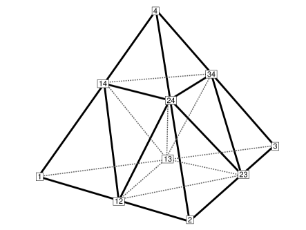
Figure 2. The original tetrahedral with vertices $(1,2,3,4)$ is divided into 8 tetrahedra with vertices $(1,12,13,14)$, $(12,2,23,24)$, $(13,23,3,34)$, $(14,24,34,4)$, $(14,12,13,24)$, $(13,12,23,24)$, $(13,23,34,24)$, $(13,34,14,24)$, where the node at vertex $ij$ is placed at the centroid of nodes at vertices $i$ and $j$.

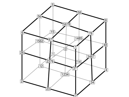
Figure 3. The original hexahedron with vertices $(1,2,3,4,5,6,7,8)$ is divided into 8 hexahedra with vertices $(15,1562,0,1485,5,56,5678,58)$, $(1485,0,3487,48,58,5678,78,8)$, $(1562,26,2376,0,56,6,67,5678)$, $(0,2376,37,3487,5678,67,7,78)$, $(1,12,1234,14,15,1562,0,1485)$, $(14,1234,34,4,1485,0,3487,48)$, $(12,2,23,1234,1562,26,2376,0)$, $(1234,23,3,34,0,2376,37,3487)$, where the new node at vertex $ijk\ell$ is placed at the centroid of nodes with vertices $i$, $j$, $k$, and $\ell$, and the new node at vertex $0$ is placed at the centroid of the nodes for all eight vertices of the original hexahedron.

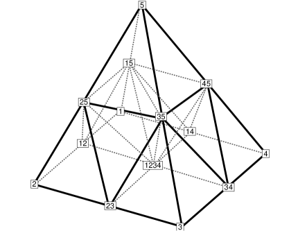
Figure 4. The original pyramid with vertices $(1,2,3,4,5)$ is divided into 4 pyramids and 8 tetrahedra with vertices $(1,12,1234,14,15)$, $(12,2,23,1234,25)$, $(1234,23,3,34,35)$, $(14,1234,34,4,45)$, $(12,15,25,1234)$, $(23,35,25,1234)$, $(34,45,35,1234)$, $(14,45,15,1234)$, $(15,25,35,5)$, $(15,35,45,5)$, $(15,35,25,1234)$, $(15,45,35,1234)$.

It is clear that a uniform refinement of a THP partition is again a THP partition.

Remark 3.

There are three choices of uniform tetrahedral refinements. Instead of choosing the diagonal edge by connecting the nodes $13$ and $24$ as shown in Figure 2, we could connect the nodes $14$ and ${23}$, or the nodes $12$ and $34$. We shall follow [28, Page 1138] to choose a particular diagonal, which guarantees the non-degeneracy of the tetrahedra in the series of THP partitions.

4.3. The global finite elements

With the finite elements on pyramids in Section 3, we are ready to construct a global lowest-order finite element exact sequence on a THP partition $\mathcal{T}_{h}$ combining with the finite elements on tetrahedra and hexahedra listed in (2a)–(2d) (and Table 1–4) in Section 1:

$$S_{h,1}= \{v\in H^{1}(\Omega): \;\;\;v\raise-0.86108pt\hbox{$|$}_{K}\in S(K),\;\;\;\forall\,K\in\mathcal{T}_{h}\}$$

$${\boldsymbol{E}}_{h,0}= \{{\boldsymbol{v}}\in H(\mathrm{curl},\Omega): \;\;\;{\boldsymbol{v}}\raise-0.86108pt\hbox{$|$}_{K}\in{\boldsymbol{E}}(K),\;\;\;\forall\,K\in\mathcal{T}_{h}\}$$

$${\boldsymbol{V}}_{h,0}= \{{\boldsymbol{v}}\in H(\mathrm{div},\Omega): \;\;\;{\boldsymbol{v}}\raise-0.86108pt\hbox{$|$}_{K}\in{\boldsymbol{V}}(K),\;\;\;\forall\,K\in\mathcal{T}_{h}\}$$

$$W_{h,0}= \{v\in L^{2}(\Omega): \;\;\;v\raise-0.86108pt\hbox{$|$}_{K}\in W(K),\;\;\;\forall\,K\in\mathcal{T}_{h}\}.$$

We define the global interpolation operators $\varPi_{S},{\boldsymbol{\varPi}}_{E},{\boldsymbol{\varPi}}_{V},$ and $\varPi_{W}$, restricted to each element to be the image of the corresponding interpolant defined on the reference element under the mapping used to define the finite elements on the physical element in terms of the finite elements on the reference element.

The global finite elements give an exact sequence on the THP partition $\mathcal{T}_{h}$ and satisfy the commuting diagram property.

Theorem 7.

(a) The sequence

$$\mathbb{R}\overset{id}{\longrightarrow}S_{h,1}\overset{{\nabla}}{\longrightarrow}{\boldsymbol{E}}_{h,0}\overset{{{\nabla\times}}}{\longrightarrow}{\boldsymbol{V}}_{h,0}\overset{{\nabla\cdot}}{\longrightarrow}W_{h,0}\overset{}{\longrightarrow}0,$$

is exact.
(b) The following diagram commutes:

where $r>3/2$.

4.4. Approximation properties

Optimal approximation properties of the above global finite elements on affine THP partitions follow directly by summing the local estimates provided in part (c) of Theorem 6 (and Remark 1). Here we prove optimal approximation properties, following [30, 20], of the global finite elements on a series of THP partitions obtained via uniform refinements of an initial coarse THP partition.

The finite elements on a physical element $K$ (tetrahedron, hexahedron, or pyramid) are defined via proper mappings from the reference element $\widehat{K}$ (reference tetrahedron (1a), reference hexahedron (1b), or reference pyramid (9)). The affine tetrahedral mapping is

$$\Phi_{K}(\widehat{x})= \;\sum_{i=1}^{4}\mathsf{v}_{i}\phi_{i},$$ (13a)

where $$\{\mathsf{v}_{i}\}_{i=1}^{4} \{\phi_{i}\}_{i=1}^{4}$$ are the vertices of the physical tetrahedron, and are the four linear nodal bases on the reference tetrahedron given in Table 1; the trilinear hexahedral mapping is

$$\Phi_{K}(\widehat{x})= \;\sum_{i=1}^{8}\mathsf{v}_{i}\phi_{i},$$ (13b)

where $\{\mathsf{v}_{i}\}_{i=1}^{8}$ are the vertices of the physical hexahedron, and $\{\phi_{i}\}_{i=1}^{8}$ are the eight trilinear nodal bases on the reference hexahedron given in Table 1; and the (composite) pyramidal mapping is given in (12).

We have the following bounds on the derivatives of the mappings on a series of uniformly refined THP partitions.

Lemma 5.

Let $\{\mathcal{T}_{h}\}_{h\downarrow 0}$ be a series of uniformly refined THP partitions of a polyhedral domain. Then,

$$\max_{i,j\in\{1,2,3\}}\left|\frac{\partial^{2}\,\Phi_{K}}{\partial\hat{x}_{i}\partial\hat{x}_{j}}\right|_{\infty,\widehat{K}}\preceq h_{K}^{2}$$

for all element $K\in\mathcal{T}_{h}$.

Proof.

We consider each type of elements in turn.

When the element $K$ is a tetrahedron, the mapping $\Phi_{K}$ is affine, and the inequality holds trivially.

When the element $K$ is a pyramid obtained by mapping a reference pyramid using the piecewise quadratic mapping (12), the second derivative of the mapping $\Phi_{K}$ is a constant in each of the tetrahedra of which it is composed, and moreover, on each such tetrahedra, we have

$$\left|\frac{\partial^{2}\,\Phi_{K}}{\partial\hat{x}_{i}\partial\hat{x}_{j}}\right|\leq|\mathsf{v}_{P}|,\quad\quad\text{ for all }i,j\in\{1,2,3\}.$$

Here $\mathsf{v}_{P}=\mathsf{v}_{1}-\mathsf{v}_{2}+\mathsf{v}_{3}-\mathsf{v}_{4}$, and $\{\mathsf{v}_{i}\}_{i=1}^{4}$ are the four vertices for the quadrilateral base of the pyramid as shown in Figure 1. Hence, in order to prove the bound in Lemma 5, it suffices to show that $|\mathsf{v}_{P}|\preceq h_{K}^{2}$.

We consider two consecutive THP partitions, $\mathcal{T}_{h}$ and $\mathcal{T}_{h/2}$, where $\mathcal{T}_{h/2}$ is obtained from $\mathcal{T}_{h}$ via a uniform refinement.

Let $K_{m}\in\mathcal{T}_{h}$ be a pyramid with vertices $(1,2,3,4,5)$, and $K_{c}\in\mathcal{T}_{h/2}$ be one of its four child pramids. Without loss of generality, we take the vertices of $K_{c}$ to be $(1,12,1234,14,5)$ as shown in Figure 4. We have

$$\mathsf{v}_{P}(K_{c})= \;\mathsf{v}_{1}-\mathsf{v}_{12}+\mathsf{v}_{1234}-\mathsf{v}_{14}$$

$$= \;\mathsf{v}_{1}-\frac{1}{2}(\mathsf{v}_{1}+\mathsf{v}_{2})+\frac{1}{4}(\mathsf{v}_{1}+\mathsf{v}_{2}+\mathsf{v}_{3}+\mathsf{v}_{4})-\frac{1}{2}(\mathsf{v}_{1}+\mathsf{v}_{4})$$

$$= \;\frac{1}{4}(\mathsf{v}_{1}-\mathsf{v}_{2}+\mathsf{v}_{3}-\mathsf{v}_{4})\;=\;\frac{1}{4}\mathsf{v}_{P}(K_{m}).$$

This means when a pyramid $K_{m}$ is subdivided, the size of each child pyramid is $1/2$ that of the mother whereas the quantity $\mathsf{v}_{P}(K_{c})$ is $(1/2)^{2}$ of the corresponding quantity $\mathsf{v}_{P}(K_{m})$. It follows by induction that $|\mathsf{v}_{P}|\preceq h_{K}^{2}$ as required.

When the element $K$ is a hexahedron obtained from the trilinear mapping (13b), each of the second cross derivatives $\frac{\partial^{2}\,\Phi_{K}}{\partial\hat{x}_{i}\partial\hat{x}_{j}}$, $i\not=j$, of the mapping $\Phi_{K}$ is a linear function, and the second derivatives $\frac{\partial^{2}\,\Phi_{K}}{\partial\hat{x}_{i}\partial\hat{x}_{i}}$ vanish identically. By symmetry, we only need to prove the bound for $\frac{\partial^{2}\,\Phi_{K}}{\partial\hat{x}_{1}\partial\hat{x}_{2}}$. Now,

$$\frac{\partial^{2}\,\Phi_{K}}{\partial\hat{x}_{1}\partial\hat{x}_{2}}=(\mathsf{v}_{1}-\mathsf{v}_{2}+\mathsf{v}_{3}-\mathsf{v}_{4})(1-\widehat{x}_{3})+(\mathsf{v}_{5}-\mathsf{v}_{6}+\mathsf{v}_{7}-\mathsf{v}_{8})\widehat{x}_{3},$$

and so, denoting $\mathsf{v}_{P}^{bot}(K):=\mathsf{v}_{1}-\mathsf{v}_{2}+\mathsf{v}_{3}-\mathsf{v}_{4}$ and $\mathsf{v}_{P}^{top}(K):=\mathsf{v}_{5}-\mathsf{v}_{6}+\mathsf{v}_{7}-\mathsf{v}_{8}$, we have

$$\left|\frac{\partial^{2}\,\Phi_{K}}{\partial\hat{x}_{1}\partial\hat{x}_{2}}\right|\leq\max\left\{|\mathsf{v}_{P}^{bot}|,|\mathsf{v}_{P}^{top}|\right\}.$$

As before, we consider two consecutive THP partitions, $\mathcal{T}_{h}$ and $\mathcal{T}_{h/2}$, and show that the right hand side of the above inequality decreases (at least) by $(1/2)^{2}$ as the mesh size decrease by $1/2$. The result then follows by induction.

Let $K_{m}\in\mathcal{T}_{h}$ be a hexahedron with vertices $(1,2,3,4,5,6,7,8)$, and $K_{c}\in\mathcal{T}_{h/2}$ be one of its eight child hexahedra. Without loss of generality, we take the vertices of $K_{c}$ to be $(15,1562,0,1485,5,56,5678,58)$ as shown in Figure 3. We have

$$\mathsf{v}_{P}^{bot}(K_{c})= \;\mathsf{v}_{15}-\mathsf{v}_{1562}+\mathsf{v}_{0}-\mathsf{v}_{1485}$$

$$= \;\frac{1}{2}(\mathsf{v}_{1}+\mathsf{v}_{5})-\frac{1}{4}(\mathsf{v}_{1}+\mathsf{v}_{5}+\mathsf{v}_{6}+\mathsf{v}_{2})+\frac{1}{8}\sum_{i=1}^{8}\mathsf{v}_{i}-\frac{1}{4}(\mathsf{v}_{1}+\mathsf{v}_{4}+\mathsf{v}_{5}+\mathsf{v}_{8})$$

$$= \;\frac{1}{8}(\mathsf{v}_{1}-\mathsf{v}_{2}+\mathsf{v}_{3}-\mathsf{v}_{4}+\mathsf{v}_{5}-\mathsf{v}_{6}+\mathsf{v}_{7}-\mathsf{v}_{8})$$

$$= \;\frac{1}{8}\left(\mathsf{v}_{P}^{bot}(K_{m})+\mathsf{v}_{P}^{top}(K_{m})\right),$$

$$\mathsf{v}_{P}^{top}(K_{c})= \;\mathsf{v}_{5}-\mathsf{v}_{56}+\mathsf{v}_{5678}-\mathsf{v}_{58}$$

$$= \;\mathsf{v}_{5}-\frac{1}{2}(\mathsf{v}_{5}+\mathsf{v}_{6})+\frac{1}{4}(\mathsf{v}_{5}+\mathsf{v}_{6}+\mathsf{v}_{7}+\mathsf{v}_{8})-\frac{1}{2}(\mathsf{v}_{5}+\mathsf{v}_{8})$$

$$= \;\frac{1}{4}\mathsf{v}_{P}^{top}(K_{m}).$$

This implies that

$$\max\left\{|\mathsf{v}_{P}^{bot}(K_{c})|,|\mathsf{v}_{P}^{top}(K_{c})|\right\}\leq\frac{1}{4}\max\left\{|\mathsf{v}_{P}^{bot}(K_{m})|,|\mathsf{v}_{P}^{top}(K_{m})|\right\}.$$

Hence, we have $|\mathsf{v}_{P}|\preceq h_{K}^{2}$ as desired. ∎

The following estimates for the Jacobian matrix and determinant of the mapping from the reference element to elements in a family of THP partitions will be useful:

Lemma 6.

Let $\{\mathcal{T}_{h}\}_{h\downarrow 0}$ be a series of uniformly refined THP partitions. Then,

$$h_{K}\preceq|F_{K}|_{0,\infty,\widehat{K}}\preceq h_{K},\quad\quad h_{K}^{3}\preceq|J_{K}|_{0,\infty,\widehat{K}}\preceq h_{K}^{3},$$ (14a)

and

$$|F_{K}|_{1,\infty,\widehat{K}}\preceq h_{K}^{2},\quad|J_{K}F_{K}^{-1}|_{1,\infty,\widehat{K}}\preceq h_{K}^{3},\quad|J_{K}|_{1,\infty,\widehat{K}}\preceq h_{K}^{4},$$ (14b)

holds for all elements $K\in\mathcal{T}_{h}$.

Proof.

Lemma 5 means that each hexahedral element in the series of THP partitions is automatically an $h^{2}$-parallelepiped in the sense defined in [20, Chapter 3]. Hence, the proof of Lemma 6 for the hexahedral case can be found in [20, Lemma 3.1]. The proof for the pyramidal case is similar and omitted, and that for the tetrahedral case is trivial. ∎

The main approximation results of the finite elements are summarized below.

Theorem 8.

Let $\{\mathcal{T}_{h}\}_{h\downarrow 0}$ be a series of uniformly refined THP partitions of a polyhedral domain $\Omega$. Then, the nodal interpolation operators have the following approximation properties:

• If $v\in H^{2}(\Omega)$, then

  $$\|v-\varPi_{S}v\|_{0}\preceq \;h^{2}\|v\|_{2},\;\;\|{\nabla}(v-\varPi_{S}v)\|_{0}\preceq \;h\|v\|_{2},$$

• If ${\boldsymbol{v}}\in H^{1}(\mathrm{curl},\Omega)$, then

  $$\|{\boldsymbol{v}}-{\boldsymbol{\varPi}}_{E}{\boldsymbol{v}}\|_{0}\preceq \;h(\|{\boldsymbol{v}}\|_{1}+\|{{\nabla\times}}{\boldsymbol{v}}\|_{1}),\;\;\|{{\nabla\times}}({\boldsymbol{v}}-{\boldsymbol{\varPi}}_{E}{\boldsymbol{v}})\|_{0}\preceq \;h\|{{\nabla\times}}{\boldsymbol{v}}\|_{1}.$$

• If ${\boldsymbol{v}}\in H^{1}(\mathrm{div},\Omega)$, then

  $$\|{\boldsymbol{v}}-{\boldsymbol{\varPi}}_{V}{\boldsymbol{v}}\|_{0}\preceq \;h\|{\boldsymbol{v}}\|_{1},\;\;\|{\nabla\cdot}({\boldsymbol{v}}-{\boldsymbol{\varPi}}_{V}{\boldsymbol{v}})\|_{0}\preceq \;h\|{\nabla\cdot}{\boldsymbol{v}}\|_{1}.$$

• If $v\in H^{1}(\Omega)$, then

  $$\|v-\varPi_{W}v\|_{0}\preceq \;h\|v\|_{1}.$$

Here $h$ is the mesh size of the THP partition $\mathcal{T}_{h}$, and all norms are evaluated on the domain $\Omega$.

Proof.

We shall prove the estimates on a single element $K$, and sum to obtain the corresponding estimates on the composite mesh.

Let $\Phi_{K}$ be the mapping from a reference element $\widehat{K}$ to a physical element $K$, and $F_{K}$ and $J_{K}$ be the corresponding Jacobian matrix and determinant, respectively.

Denote $\widehat{\varPi}_{S}$, $\widehat{{\boldsymbol{\varPi}}}_{E}$, $\widehat{{\boldsymbol{\varPi}}}_{V}$, and $\widehat{\varPi}_{W}$, respectively, be the nodal interpolators for the $H^{1}$, $H(\mathrm{curl})$, $H(\mathrm{div})$, and $L^{2}$ finite elements on the reference element, respectively.

We first prove the estimates in the $L^{2}$-norm for each of the spaces $S_{h,1}$, ${\boldsymbol{E}}_{h,0}$, ${\boldsymbol{V}}_{h,0}$, and $W_{h,0}$.

The proof for $S_{h,1}$ follows line-by-line from [30, Lemma 1]. For a given function $v\in H^{2}(K)$ on $K$, we associate the function $\widehat{v}\equiv v\circ\Phi_{K}\in H^{2}(\widehat{K})$. Thanks to Theorem 6(c) part (1) and Remark 1, there holds

$$\|\widehat{v}-\widehat{\varPi}_{S}\widehat{v}\|_{\widehat{K}}\preceq|\widehat{v}|_{2,\widehat{K}},$$

and hence, observing the relation $\varPi_{S}v({\boldsymbol{x}})=\widehat{\varPi}_{S}\widehat{v}(\widehat{{\boldsymbol{x}}})$ and using the bound for the determinant $J_{K}$ in (14a), it follows that

$$\|v-\varPi_{S}v\|_{K}\preceq h_{K}^{3/2}\|v-\varPi_{S}v\|_{\widehat{K}}\preceq h_{K}^{3/2}|\widehat{v}|_{2,\widehat{K}}.$$

To estimate the term on the right hand side, we note that

$$|\widehat{\nabla}^{2}\widehat{v}|=|\widehat{\nabla}(F_{K}^{T}\nabla v)|\preceq|F_{K}|_{1,\infty}|\nabla v|+|F_{K}|^{2}_{0,\infty}|\nabla^{2}v|\preceq h_{K}^{2}(|\nabla v|+|\nabla^{2}v|),$$

where the last inequality follows from the estimates in Lemma 6. This yields

$$\|v-\varPi_{S}v\|_{K}\preceq h_{K}^{2}\|v\|_{2,K}.$$

The proof for ${\boldsymbol{E}}_{h,0}$ follows using a similar argument to the tetrahedral case given in [24, Theorem 5.41]. For a given ${\boldsymbol{v}}\in H^{1}(\mathrm{curl};K)$ on $K$, we associate the function $\widehat{{\boldsymbol{v}}}\equiv F_{K}^{T}{\boldsymbol{v}}\circ\Phi_{K}\in H^{1}(\mathrm{curl};\widehat{K})$. By Theorem 6(c) part (2) and Remark 1, we have

$$\|\widehat{{\boldsymbol{v}}}-\widehat{{\boldsymbol{\varPi}}}_{E}\widehat{{\boldsymbol{v}}}\|_{\widehat{K}}\preceq|\widehat{{\boldsymbol{v}}}|_{1,\widehat{K}}+|\widehat{\nabla}\times\widehat{{\boldsymbol{v}}}|_{1,\widehat{K}}.$$

Hence, using the relation ${\boldsymbol{\varPi}}_{E}{\boldsymbol{v}}({\boldsymbol{x}})=F_{K}^{-T}\widehat{{\boldsymbol{\varPi}}}_{E}\widehat{{\boldsymbol{v}}}(\widehat{{\boldsymbol{x}}})$ and using the bound for the Jacobian $F_{K}$ and determinant $J_{K}$ in (14a), it follows that

$$\|{\boldsymbol{v}}-{\boldsymbol{\varPi}}_{E}{\boldsymbol{v}}\|_{K}\preceq h_{K}^{1/2}\|\widehat{{\boldsymbol{v}}}-\widehat{{\boldsymbol{\varPi}}}_{E}\widehat{{\boldsymbol{v}}}\|_{\widehat{K}}\preceq h_{K}^{1/2}(|\widehat{{\boldsymbol{v}}}|_{1,\widehat{K}}+|\widehat{\nabla}\times\widehat{{\boldsymbol{v}}}|_{1,\widehat{K}}).$$

The term on the right hand side can be estimated by noting that

$$|\widehat{\nabla}\widehat{{\boldsymbol{v}}}|\preceq|F_{K}|_{1,\infty}|{\boldsymbol{v}}|+|F_{K}|^{2}_{0,\infty}|\nabla{\boldsymbol{v}}|\preceq h_{K}^{2}(|{\boldsymbol{v}}|+|\nabla{\boldsymbol{v}}|),$$

and then

$$|\widehat{\nabla}(\widehat{\nabla}\times\widehat{{\boldsymbol{v}}})|\preceq \;|J_{K}F_{K}^{-1}|_{1,\infty}|\nabla\times{\boldsymbol{v}}|+|J_{K}F_{K}^{-1}|_{0,\infty}|F_{K}|_{0,\infty}|{\nabla}(\nabla\times{\boldsymbol{v}})|$$

$$\preceq \;h_{K}^{3}(|\nabla\times{\boldsymbol{v}}|+|\nabla(\nabla\times{\boldsymbol{v}})|),$$

thanks to the relation $\widehat{\nabla}\times\widehat{{\boldsymbol{v}}}=J_{K}F_{K}^{-1}\nabla\times{\boldsymbol{v}}$. Hence,

$$\|{\boldsymbol{v}}-{\boldsymbol{\varPi}}_{E}{\boldsymbol{v}}\|_{K}\preceq h_{K}(\|{\boldsymbol{v}}\|_{1,K}+h_{K}\|\nabla\times{\boldsymbol{v}}\|_{1,K}).$$

Let us now prove the $L^{2}$-estimate for ${\boldsymbol{V}}_{h,0}$. For a given function ${\boldsymbol{v}}\in H^{1}(\mathrm{div};K)$ on $K$, we associate the function $\widehat{{\boldsymbol{v}}}\equiv J_{K}F_{K}^{-1}{\boldsymbol{v}}\circ\Phi_{K}\in H^{1}(\mathrm{curl};\widehat{K})$. By Theorem 6(c) part (3) and Remark 1, we have

$$\|\widehat{{\boldsymbol{v}}}-\widehat{{\boldsymbol{\varPi}}}_{V}\widehat{{\boldsymbol{v}}}\|_{\widehat{K}}\preceq|\widehat{{\boldsymbol{v}}}|_{1,\widehat{K}}.$$

Hence, using the relation ${\boldsymbol{\varPi}}_{V}{\boldsymbol{v}}({\boldsymbol{x}})=J_{K}^{-1}F_{K}\widehat{{\boldsymbol{\varPi}}}_{V}\widehat{{\boldsymbol{v}}}(\widehat{{\boldsymbol{x}}})$ and using the bound for the Jacobian $F_{K}$ and determinant $J_{K}$ in (14a), it follows that

$$\|{\boldsymbol{v}}-{\boldsymbol{\varPi}}_{V}{\boldsymbol{v}}\|_{K}\preceq h_{K}^{-1/2}\|\widehat{{\boldsymbol{v}}}-\widehat{{\boldsymbol{\varPi}}}_{V}\widehat{{\boldsymbol{v}}}\|_{\widehat{K}}\preceq h_{K}^{-1/2}|\widehat{{\boldsymbol{v}}}|_{1,\widehat{K}}.$$

An estimate of the term on the right hand side follows in the same way as in the $H(\mathrm{curl})$ case:

$$|\widehat{\nabla}\widehat{{\boldsymbol{v}}}|\preceq \;|J_{K}F_{K}^{-1}|_{1,\infty}|{\boldsymbol{v}}|+|J_{K}F_{K}^{-1}|_{0,\infty}|F_{K}|_{0,\infty}|{\nabla}{\boldsymbol{v}}|\preceq\;h_{K}^{3}(|{\boldsymbol{v}}|+|\nabla{\boldsymbol{v}}|),$$

so that

$$\|{\boldsymbol{v}}-{\boldsymbol{\varPi}}_{V}{\boldsymbol{v}}\|_{K}\preceq h_{K}\|{\boldsymbol{v}}\|_{1,K}.$$

Finally, we prove the $L^{2}$-estimate for $W_{h,0}$. For a given function $v\in H^{1}(K)$ on $K$, we associate the function $\widehat{{\boldsymbol{v}}}\equiv J_{K}v\circ\Phi_{K}\in H^{1}(\widehat{K})$. By Theorem 6(c) part (4) and Remark 1, we have

$$\|\widehat{v}-\widehat{\varPi}_{W}\widehat{v}\|_{\widehat{K}}\preceq|\widehat{v}|_{1,\widehat{K}}.$$

Hence, observing the relation $\varPi_{W}v({\boldsymbol{x}})=J_{K}^{-1}\widehat{\varPi}_{W}\widehat{v}(\widehat{{\boldsymbol{x}}})$ and using the bound for the determinant $J_{K}$ in (14a), it follows that

$$\|v-\varPi_{W}v\|_{K}\preceq h_{K}^{-3/2}\|\widehat{v}-\widehat{\varPi}_{W}\widehat{v}\|_{\widehat{K}}\preceq h_{K}^{-3/2}|\widehat{v}|_{1,\widehat{K}}.$$

To estimate the term on the right hand side, we note that

$$|\widehat{\nabla}\widehat{v}|\preceq \;|J_{K}|_{1,\infty}|v|+|J_{K}|_{0,\infty}|F_{K}|_{0,\infty}|{\nabla}v|\preceq\;h_{K}^{4}(|v|+|\nabla v|),$$

and hence

$$\|v-\varPi_{W}v\|_{K}\preceq h_{K}\|v\|_{1,K}.$$

It remains to prove the estimates (1)–(4) for the derivatives. In fact, these estimates are immediate consequence of the commuting diagram property. In particular, observing ${\nabla}\varPi_{S}=\varPi_{E}{\nabla}$, there holds

$$\|{\nabla}(v-\varPi_{S}v)\|_{K}=\|{\nabla}v-{\boldsymbol{\varPi}}_{E}{\nabla}v\|_{K}\preceq \;h_{K}\|{\nabla}v\|_{1,K},$$

observing ${{\nabla\times}}{\boldsymbol{\varPi}}_{E}={\boldsymbol{\varPi}}_{V}{{\nabla\times}}$, there holds

$$\|{{\nabla\times}}({\boldsymbol{v}}-{\boldsymbol{\varPi}}_{E}{\boldsymbol{v}})\|_{K}=\|{{\nabla\times}}{\boldsymbol{v}}-{\boldsymbol{\varPi}}_{V}({{\nabla\times}}{\boldsymbol{v}})\|_{K}\preceq \;h_{K}\|{{\nabla\times}}{\boldsymbol{v}}\|_{1,K},$$

while observing ${\nabla\cdot}{\boldsymbol{\varPi}}_{V}=\varPi_{W}{\nabla\cdot}$, there holds

$$\|{\nabla\cdot}({\boldsymbol{v}}-{\boldsymbol{\varPi}}_{V}{\boldsymbol{v}})\|_{K}=\|{\nabla\cdot}{\boldsymbol{v}}-\varPi_{W}({\nabla\cdot}{\boldsymbol{v}})\|_{K}\preceq \;h_{K}\|{\nabla\cdot}{\boldsymbol{v}}\|_{1,K}.$$

∎

5. Conclusion

In this paper, we introduced a set of lowest-order composite finite elements for the de Rham complex on pyramids. The finite elements are compatible with those for the lowest-order Raviart-Thomas-Nédélec sequence on tetrahedra and hexahedra, and, as such, can be used to construct conforming finite element spaces on THP partitions consisting of tetrahedra, pyramids, and hexahedra. Moreover, the finite element spaces deliver optimal error estimates on a sequence of successively refined THP partitions.

References

- [1] M. Ainsworth, O. Davydov, and L. L. Schumaker, Bernstein-Bézier finite elements on tetrahedral-hexahedral-pyramidal partitions, Comput. Methods Appl. Mech. Engrg., 304 (2016), pp. 140–170.
- [2] D. N. Arnold and A. Logg, Periodic Table of the Finite Elements, SIAM News, 47 (2014).
- [3] T. C. Baudouin, J.-F. Remacle, E. Marchandise, F. Henrotte, and C. Geuzaine, A frontal approach to hex-dominant mesh generation, Adv. Model. Simul. Eng. Sci., 1:8 (2014), pp. 1–30.
- [4] G. Bedrosian, Shape functions and integration formulas for three-dimensional finite element analysis, Internat. J. Numer. Methods Engrg., 35 (1992), pp. 95–108.
- [5] M. Bergot, G. Cohen, and M. Duruflé, Higher-order finite elements for hybrid meshes using new nodal pyramidal elements, J. Sci. Comput., 42 (2010), pp. 345–381.
- [6] M. Bergot and M. Duruflé, Approximation of with high-order optimal finite elements for pyramids, prisms and hexahedra, Commun. Comput. Phys., 14 (2013), pp. 1372–1414.
- [7] , High-order optimal edge elements for pyramids, prisms and hexahedra, J. Comput. Phys., 232 (2013), pp. 189–213.
- [8] , Higher-order discontinuous Galerkin method for pyramidal elements using orthogonal bases, Numer. Methods Partial Differential Equations, 29 (2013), pp. 144–169.
- [9] M. J. Bluck and S. P. Walker, Polynomial basis functions on pyramidal elements, Comm. Numer. Methods Engrg., 24 (2008), pp. 1827–1837.
- [10] A. Bossavit, Computational electromagnetism, Electromagnetism, Academic Press, Inc., San Diego, CA, 1998. Variational formulations, complementarity, edge elements.
- [11] S. C. Brenner and L. R. Scott, The mathematical theory of finite element methods, vol. 15 of Texts in Applied Mathematics, Springer, New York, third ed., 2008.
- [12] J. Chan and T. Warburton, A comparison of high order interpolation nodes for the pyramid, SIAM J. Sci. Comput., 37 (2015), pp. A2151–A2170.
- [13] , A short note on a Bernstein-Bezier basis for the pyramid, SIAM J. Sci. Comput., 38 (2016), pp. A2162–A2172.
- [14] P. G. Ciarlet, The finite element method for elliptic problems, North-Holland Publishing Co., Amsterdam-New York-Oxford, 1978. Studies in Mathematics and its Applications, Vol. 4.
- [15] B. Cockburn and G. Fu, A systematic construction of finite element commuting exact sequences, SIAM J. Numer. Anal., (2017). To appear.
- [16] L. Demkowicz and A. Buffa, , and -conforming projection-based interpolation in three dimensions. Quasi-optimal -interpolation estimates, Comput. Methods Appl. Mech. Engrg., 194 (2005), pp. 267–296.
- [17] F. Fuentes, B. Keith, L. Demkowicz, and S. Nagaraj, Orientation embedded high order shape functions for the exact sequence elements of all shapes, Comput. Math. Appl., 70 (2015), pp. 353–458.
- [18] A. Gillette, Serendipity and tensor product pyramid finite elements, SMAI Journal of Computational Mathematics, 2 (2016), pp. 215–228.
- [19] V. Gradinaru and R. Hiptmair, Whitney elements on pyramids, Electron. Trans. Numer. Anal., 8 (1999), pp. 154–168.
- [20] R. Ingram, M. F. Wheeler, and I. Yotov, A multipoint flux mixed finite element method on hexahedra, SIAM J. Numer. Anal., 48 (2010), pp. 1281–1312.
- [21] P. Knabner and G. Summ, The invertibility of the isoparametric mapping for pyramidal and prismatic finite elements, Numer. Math., 88 (2001), pp. 661–681.
- [22] L. Liu, K. B. Davies, M. Kří žek, and L. Guan, On higher order pyramidal finite elements, Adv. Appl. Math. Mech., 3 (2011), pp. 131–140.
- [23] L. Liu, K. B. Davies, K. Yuan, and M. Kří žek, On symmetric pyramidal finite elements, Dyn. Contin. Discrete Impuls. Syst. Ser. B Appl. Algorithms, 11 (2004), pp. 213–227. First Industrial Mathematics Session.
- [24] P. Monk, Finite element methods for Maxwell’s equations, Numerical Mathematics and Scientific Computation, Oxford University Press, New York, 2003.
- [25] J.-C. Nédélec, Mixed finite elements in , Numer. Math., 35 (1980), pp. 315–341.
- [26] N. Nigam and J. Phillips, High-order conforming finite elements on pyramids, IMA J. Numer. Anal., 32 (2012), pp. 448–483.
- [27] , Numerical integration for high order pyramidal finite elements, ESAIM Math. Model. Numer. Anal., 46 (2012), pp. 239–263.
- [28] M. E. Ong, Uniform refinement of a tetrahedron, SIAM J. Sci. Comput., 15 (1994), pp. 1134–1144.
- [29] S. J. Owen and S. Saigal, Formation of pyramid elements for hexahedra to tetrahedra transitions, Comput. Methods Appl. Mech. Engrg., 190 (2001), pp. 4505–4518.
- [30] R. Rannacher and S. Turek, Simple nonconforming quadrilateral Stokes element, Numer. Methods Partial Differential Equations, 8 (1992), pp. 97–111.
- [31] J. Schöberl, A posteriori error estimates for Maxwell equations, Math. Comp., 77 (2008), pp. 633–649.
- [32] S. J. Sherwin, Hierarchical finite elements in hybrid domains, Finite Elem. Anal. Des., 27 (1997), pp. 109–119.
- [33] S. J. Sherwin, T. Warburton, and G. E. Karniadakis, Spectral/ methods for elliptic problems on hybrid grids, in Domain decomposition methods, 10 (Boulder, CO, 1997), vol. 218 of Contemp. Math., Amer. Math. Soc., Providence, RI, 1998, pp. 191–216.
- [34] T. Warburton, Application of the discontinuous Galerkin method to Maxwell’s equations using unstructured polymorphic -finite elements, in Discontinuous Galerkin methods (Newport, RI, 1999), vol. 11 of Lect. Notes Comput. Sci. Eng., Springer, Berlin, 2000, pp. 451–458.
- [35] C. Wieners, Conforming Discretizations on tetrahedrons, pyramids, prisms and hexahedrons, (1997). preprint Bericht 97/15, University of Stuttgart.