On the sub-Gaussianity of the Beta and Dirichlet distributions
Abstract
We obtain the optimal proxy variance for the sub-Gaussianity of Beta distribution, thus proving upper bounds recently conjectured by Elder (2016). We provide different proof techniques for the symmetrical (around its mean) case and the non-symmetrical case. The technique in the latter case relies on studying the ordinary differential equation satisfied by the Beta moment-generating function known as the confluent hypergeometric function. As a consequence, we derive the optimal proxy variance for the Dirichlet distribution, which is apparently a novel result. We also provide a new proof of the optimal proxy variance for the Bernoulli distribution, and discuss in this context the proxy variance relation to log-Sobolev inequalities and transport inequalities.
1 Introduction
The sub-Gaussian property (Buldygin and Kozachenko,, 1980, 2000; Pisier,, 2016) and related concentration inequalities (Boucheron et al.,, 2013; Raginsky and Sason,, 2013) have attracted a lot of attention in the last couple of decades due to their applications in various areas such as pure mathematics, physics, information theory and computer sciences. Recent interest focused on deriving the optimal proxy variance for discrete random variables like the Bernoulli distribution (Buldygin and Moskvichova,, 2013; Kearns and Saul,, 1998; Berend and Kontorovich,, 2013) and the missing mass (McAllester and Schapire,, 2000; McAllester and Ortiz,, 2003; Berend and Kontorovich,, 2013; Ben-Hamou et al.,, 2017). Our focus is instead on two continuous random variables, the Beta and Dirichlet distributions, for which the optimal proxy variance was not known to the best of our knowledge. Some upper bounds were recently conjectured by Elder, (2016) that we prove in the present article by providing the optimal proxy variance for both Beta and Dirichlet distributions. Similar concentration properties of the Beta distribution have been recently used in many contexts including Bayesian adaptive data analysis (Elder,, 2016), Bayesian nonparametrics (Castillo,, 2016) and spectral properties of random matrices (Perry et al.,, 2016).
We start by reminding the definition of sub-Gaussian property for random variables:
Definition 1 (Sub-Gaussian variables).
A random variable with finite mean is sub-Gaussian if there is a positive number such that:
| (1) |
Such a constant is called a proxy variance (or sub-Gaussian norm), and we say that is -sub-Gaussian. If is sub-Gaussian, one is usually interested in the optimal proxy variance:
Note that the variance always gives a lower bound on the optimal proxy variance: . In particular, when , is said to be strictly sub-Gaussian.
Every compactly supported distribution, as is the Beta distribution, is sub-Gaussian. This can be seen by Hoeffding’s classic inequality: any random variable supported on with mean satisfies
thus exhibiting as an upper bound to the proxy variance. This bound can be improved by taking into account the location of the mean within the interval . An early step in this direction is the second inequality in Hoeffding, (1963) paper, indexed (2.2). It states that if , then for any positive , , where
| (2) |
thus indicating that has a right tail lighter than a Gaussian tail of variance . Hoeffding’s result was strengthened by Kearns and Saul, (1998) to comply with Definition 1 of sub-Gaussianity111Note indeed that Equation (1), together with Markov inequality, imply . as follows
| (3) |
thus indicating that is a distribution-sensitive proxy variance for any -supported random variable with mean (see also Berend and Kontorovich,, 2013, for a detailed proof of this result). If this is the optimal proxy variance for the Bernoulli distribution (see Theorem 2.1 and Theorem 3.1 of Buldygin and Moskvichova,, 2013), it is clear from our result that it does not hold true for the Beta distribution. However, fixing and letting , , the distribution concentrates to the distribution, and we show that we recover the optimal proxy variance for the Bernoulli distribution (Theorem 2).
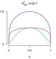
An interesting common feature between optimal proxy variances for the Bernoulli distribution: , and that of the Beta distribution derived later on, is that they deteriorate in a similar fashion as the mean goes to 0 or 1, see for instance the left panel of Figure 1. We briefly present here classical proof techniques for sub-Gaussianity hinging on certain tools from functional analysis. We show how they apply in the Bernoulli setting, and let as an interesting open problem how our proof in the Beta distribution setting could be supplemented by these same functional analysis tools.
Essentially two (related) functional inequalities allow one to derive a sub-Gaussian property: log-Sobolev inequalities, which date back to Gross, (1975), and transport inequalities. The relation with the former inequalities is called Herbst’s argument. It states that if a probability measure satisfies a log-Sobolev inequality with some constant, then it is sub-Gaussian with the same constant as a proxy variance222The implied predicate is actually stronger than sub-Gaussianity, but it is not useful for our purposes. (see for instance Ledoux,, 1999, Section 2.3 and Proposition 2.3). The optimal constant in the log-Sobolev inequality satisfied by the Bernoulli distribution also produces its optimal proxy variance (Ledoux,, 1999, Corollary 5.9).
The relation with transport inequalities is usually referred to as Marton’s argument (see for instance Raginsky and Sason,, 2013, Section 3.4). Define the Wasserstein distance between two probability measures and on a space by
where is the set of probability measures on with fixed marginal distributions respectively and . The Wasserstein distance depends on some choice of a distance on . A probability measure is said to satisfy a transport inequality with constant , if for any probability measure dominated by ,
| (4) |
where is the entropy, or Kullback–Leibler divergence, between and . The transport inequality (4) is denoted by .
Bobkov and Götze, (1999) proved that implies -sub-Gaussianity. See also Proposition 3.6 and Theorem 3.4.4 of Raginsky and Sason, (2013) for general results. Further developments in the discrete setting are interesting for our purposes. Equip a discrete space with the Hamming metric, . The induced Wasserstein distance then reduces to the total variation distance, . In that setting, Ordentlich and Weinberger, (2005) proved the distribution-sensitive transport inequality:
| (5) |
where the function is defined in Equation (2) and the coefficient is called the balance coefficient of , and is defined by . In particular, the Bernoulli balance coefficient is easily shown to coincide with its mean. Hence, applying the result of Bobkov and Götze, (1999) to the transport inequality (5) yields a distribution-sensitive proxy variance of for the Bernoulli with mean . It is optimal, see for instance Theorem 3.4.6 of Raginsky and Sason, (2013). This viewpoint highlights the key role played by the balance coefficient in the non-uniformity of the optimal proxy variance for discrete distributions such as the Bernoulli. However, it is not clear how this argument would carry over to non discrete distributions such as the Beta distribution for explaining similar sensitivity to the mean. However, to quote Raginsky and Sason, (2013), the general approach may not produce optimal concentration estimates, that often require case-by-case treatments. This is the route followed in this note for the Beta distribution.
The outline of the note is as follows. We introduce the Beta distribution and state the main result (Theorem 1) in Section 2.1. We then prove our result depending on whether (Section 2.2) or (Section 2.3). In the first case, the proof is elementary and based on comparing the coefficients of the entire series representations of the functions of both sides of inequality (1). However, it does not directly carry over to the second case, whose proof requires some finer analysis tool: the study of the ordinary differential equation (ODE) satisfied by the confluent hypergeometric function . Although the second proof also covers the case upon slight modifications, the independent proof for the symmetric case is kept owing to its simplicity. As a by-product, we derive the optimal proxy variance for the Bernoulli and the Dirichlet distributions in Section 3. The R code for the plots presented in this note and for a function deriving the optimal proxy variance in terms of and is available at http://www.julyanarbel.com/software.
2 Optimal proxy variance for the Beta distribution
2.1 Notations and main result
The distribution, with , is characterized by a density on the segment given by:
where is the Beta function. The moment-generating function of a distribution is given by a confluent hypergeometric function (also known as Kummer’s function):
| (6) |
This is equivalent to say that the raw moment of a random variable is given by:
| (7) |
where is the Pochhammer symbol, also known in the literature as a rising factorial. In particular, the mean and variance are given by:
The Beta distribution is ubiquitous in statistics. It plays a central role in the binomial model in Bayesian statistics where it is a conjugate prior distribution (the associated posterior distribution is also Beta): if and , then . It is also key to Bayesian nonparametrics where it embodies, among others, the distribution of the breaks in the stick-breaking representation of the Dirichlet process and the Pitman–Yor process; marginal distributions of Polya trees (Castillo,, 2016); the posterior distribution of discovery probabilities under a Bayesian nonparametrics model (Arbel et al.,, 2017). Our main result opens new research avenues for instance about asymptotic (frequentist) assessments of these procedures.
Our main result regarding the Beta distribution is the following:
Theorem 1 (Optimal proxy variance for the Beta distribution).
For any , the Beta distribution is -sub-Gaussian with optimal proxy variance given by:
| (8) |
A simple and explicit upper bound to
is given by :
- for we have
- for we have .
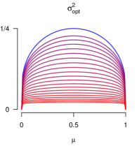
Equation (8) defining is a transcendental equation, the solution of which is not available in closed form. However, it is simple to evaluate numerically. The values of the variance, optimal proxy variance and its simple upper bound are illustrated on Figure 1. Note that for a fixed value of the sum of the parameters, , the optimal proxy variance deteriorates when , or equivalently , gets close to 0 or to . This is reminiscent of the Bernoulli optimal proxy variance behavior which deteriorates when the success probability moves away from (Buldygin and Moskvichova,, 2013).
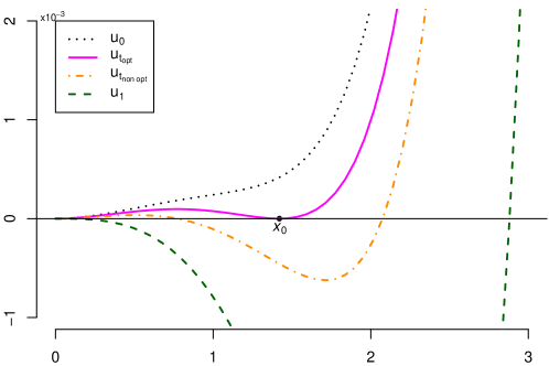
The intuition of the proof can be seen from Figure 2 (Section 2.3.3) where we represent the difference for various values of . The main argument is that the optimal proxy variance is obtained for the curve (in magenta) whose positive local minimum equals zero, thus leading to the system of equations of Theorem 1.
Corollary 1.
The Beta distribution is strictly sub-Gaussian if and only if .
As a direct consequence, we obtain the strict sub-Gaussianity of the uniform, the arc-sine and the Wigner semicircle distributions, as special cases up to a trivial rescaling of the Beta distribution respectively with equal to , and .
2.2 The distribution is strictly sub-Gaussian
Let . Since a random variable is symmetric around , only its even centered moments are non-zero. The reason why is because the coefficients of the series expansions at of each side:
| (9) | ||||
| (10) |
satisfy the inequalities:
| (11) |
Indeed, algebra yields:
| (12) |
Combining the expression of the raw moments (7) with the following inequality:
| (13) |
in (9) concludes the proof.
Remark 1.
The non-symmetrical distribution with has even centered moments whose expressions are not as simple as (12). Moreover, it has obviously non-zero odd centered moments. For this last reason, the present proof does not carry over to the case .
2.3 Optimal proxy variance for the distribution
2.3.1 Connection with ordinary differential equations
In this section, we assume that with . We denote (we omit the dependence on and for compactness) and define for all :
In other words, the decreasing function maps the interval to the interval with . Then, we introduce the function defined by:
where -sub-Gaussianity amounts to non negativity of on . Since the confluent hypergeometric function satisfies the linear second order ordinary differential equation , we obtain together with equation (6) that is the unique solution of the Cauchy problem:
| (14) |
where is a polynomial of degree in :
For normalization purposes, we also define:
| (15) |
The function is the unique solution of the Cauchy problem:
| (18) |
with:
Note that and have the same sign hence proving that is positive (resp. negative) is equivalent to proving that is positive (resp. negative). From standard theory on ODEs (Birkhoff and Rota,, 1989; Robinson,, 2004), we get that the functions and are . Indeed, the only possible singularity is at but the initial conditions imply that the function is regular at this point. In particular, a Taylor expansion at shows that:
| (19) |
We also observe that the discriminant of the polynomial is given by:
Hence we conclude that for , admits two distinct real zeros that are positive, while for it remains strictly positive on . For , admits a double zero and thus remains positive on appart from its zero.
By definition (15), we want to study the sign of on . Indeed, showing that is positive on then is equivalent to showing -sub-Gaussianity. We first observe that we may restrict the sign study on . Indeed, if we prove that:
| (20) |
then, the case is automatically obtained by noting that , whose mean is . Therefore, applying (20) to gives that for all :
Eventually, in agreement with the general theory, we observe that for (i.e. ), is not -sub-Gaussian. Indeed, the series expansion at (19), shows that for , is strictly negative in a neighborhood of . On the contrary, for , the function is strictly positive in a neighborhood of so that we may not directly conclude. Note also that for any value of , we always have .
2.3.2 Proof that the distribution is -sub-Gaussian
In this section, we take . As explained above, this corresponds to a case where is positive on (apart from its double zero). We prove that for by proceeding by contradiction. Let us assume that there exists such that . Since the non-empty set is compact (because ) and excludes a neighborhood of , we may define . Let us now define the set:
Since and the facts that is strictly positive in a neighborhood of and is continuous on , Rolle’s theorem shows that is not empty and that:
Evaluating the ODE (14) at and using the fact that the polynomial is positive on (appart from its double zero) leads to:
| (21) |
However, combined with , this contradicts the fact that changes sign at .
Thus, we conclude that there cannot exist such that . Since is strictly positive in a neighborhood of and continuous on , we conclude that it must remain strictly positive on .
Remark 2.
In this proof, the case requires an adaptation since . Thus, we must determine ( by symmetry) to ensure that the function is locally convex and remains strictly positive in a neighborhood of . Apart from this minor verification, the rest of the proof applies also to this case.
2.3.3 Proof of the optimal proxy variance for the distribution
In this section we assume that . From general theorems regarding ODEs, we have that the application:
| (22) |
is smooth (). Indeed, the -dependence of the coefficients of the ODE (18) is polynomial and thus smooth. The -dependence of the coefficients of the ODE (18) is polynomial and as explained above, the only possible singularity in is at but initial conditions ensure that the solutions are always regular there. Since for all we have , we also have that the function:
is continuous.
We now observe that for any , the functions are strictly positive in a neighborhood of . More precisely, if we choose a segment with , then for all we have that . Hence, we may choose such that for all , we have is strictly positive on . Moreover, since , is bounded from below on by a constant . Thus, since is continuous, there exists a neighborhood of in which all solutions remain greater than on and thus strictly positive on . This shows that for , is not optimal.
Let us now introduce the set:
Then, from the results presented above, we know that is non-empty, that it contains a neighborhood of and that it is bounded from above by . Moreover, by connection with the initial problem (15), is an interval and thus is of the form with . Indeed implies by construction that for all , . Note also that since is strictly negative in a neighborhood of and thus . Hence, the continuity of shows that there exists a neighborhood of in which the solutions are non-positive on . For the function must have a zero on otherwise by continuity of we may find a neighborhood of for which remains strictly positive thus contradicting the maximality of . Since must remain positive, the zero is at least a double zero and therefore we find that there exists such that , and . From (6) and (15), the conditions , are equivalent to the following system of equations (we use here the contiguous relations for the confluent hypergeometric function: ):
| (23) |
This is equivalent to say that is the solution of the transcendental equation:
and that is given by:
Note that by symmetry, we have hence, . Moreover, if then while implies . We may illustrate the situation with Figure 2 which displays the difference function .
Remark 3.
The system of equations (23) admits only one solution on . Indeed, let us transpose the problem from to using (15) and assume that there exist two points such that , and , with strictly positive on (hence and ). Using (14), this implies that and . If we denote the potential distinct positive zeros of we may exclude that . Indeed, if then we may apply the same argument to on the interval as the one developed for in Section 2.3.2 and obtain a contradiction. Thus, the only remaining case is to assume . In that case, since , , and is positive on , we may apply the same argument to on the interval as the one developed for in Section 2.3.2 and obtain a contradiction.
3 Relations to other distributions
3.1 Optimal proxy variance for the Bernoulli distribution
We show that our proof technique can be used to recover the optimal proxy variance for the Bernoulli distribution, known since Kearns and Saul, (1998). This is illustrated by the center panel of Figure 1.
Theorem 2 (Optimal proxy variance for the Bernoulli distribution).
For any , the Bernoulli distribution with mean is sub-Gaussian with optimal proxy variance given by:
| (24) |
Proof.
In the limit with fixed equal to , the differential equation (14) simplifies into:
with the Cauchy initial conditions and . The solution of this Cauchy problem is explicit and given by:
| (25) |
Therefore the optimal proxy variance is given by where is determined by the system of equations: and , thus defining implicitly and as functions of . In order to solve explicitly the last system of equations, we perform the change of variables: so that the solution (25) is now given by:
Consequently, we have to solve the system:
Introducing another change of variable , the last system is equivalent to:
We now observe that and is a solution of the former system. Performing back the various changes of variables, this is equivalent to say that so that or equivalently . Consequently, the optimal proxy variance is given by:
which is precisely the optimal proxy variance of a Bernoulli random variable with mean . ∎
3.2 Optimal proxy variance for the Dirichlet distribution
We start by reminding the definition of sub-Gaussian property for random vectors:
Definition 2 (Sub-Gaussian vectors).
A random -dimensional vector with finite mean is -sub-Gaussian if the random variable is -sub-Gaussian for any unit vector in the simplex . This is equivalent to say that:
where . Eventually, a random vector is said to be strictly sub-Gaussian, if the random variables are strictly sub-Gaussian for any unit vector .
Let . The Dirichlet distribution , with positive parameters , is characterized by a density on the simplex given by:
where and . It generalizes the Beta distribution in the sense that the components are Beta distributed. More precisely, for any non-empty and strict subset of :
However, we remind the reader that the components are not independent and the variance/covariance matrix is given by:
Eventually, if we define , then the moments of the Dirichlet distribution are given by:
This is equivalent to say that the moment-generating function of the Dirichlet distribution is:
where we have defined and
Let us define the canonical vector of and . From Definition 1 and the results regarding the distribution obtained in Section 2.3, we immediately get that is -sub-Gaussian with defined from Theorem 1. Moreover, in direction , is the optimal proxy variance. Therefore, the remaining issue is to generalize these results for arbitrary unit vectors on . We obtain the following result:
Theorem 3 (Optimal proxy variance for the Dirichlet distribution).
For any parameter , the Dirichlet distribution is sub-Gaussian with optimal proxy variance given from Theorem 1 and:
Proof.
We first observe that the computations of correspond to cases where the sum is fixed to and thus independent of . Therefore, is maximal when is minimal, i.e. when the distance from to is minimal. It is easy to see that this corresponds to choosing (by looking at the two possible cases and ).
We then observe that cannot be improved. Indeed, let us denote one of the components for which the maximum is obtained. Then, if we take , the discussion presented above shows that is the optimal proxy variance in this direction. Hence the optimal proxy variance cannot be lower than .
Let us now prove that is -sub-Gaussian. Let be a unit vector on and . We define for clarity . We have:
| (26) |
Note that we also have:
| (27) |
Moreover we have the inequality:
because both sides have the same number of terms in the product (i.e. ) but those of the right hand side are always greater or equal to those of the left hand side. Hence, from (26) and (27), we find:
Using the optimal proxy variance of the Beta distribution proven in Theorem 1, we find:
thus showing that is -sub-Gaussian and concluding the proof. ∎
Note that using Theorem 3, we obtain the following corollary:
Corollary 2.
For any integer , the Dirichlet distribution is strictly sub-Gaussian if and only if and .
Indeed, we first need to require so that all directions have the same optimal proxy variance. Then, each component satisfies and Theorem 1 shows that is the optimal proxy variance for if and only if , i.e. if and only if .
Acknowledgments
We wish to thank Stéphane Boucheron for an enlightening discussion of our results and an anonymous referee for insightful suggestions. O.M. would like to thank Université de Lyon, Université Jean Monnet and Institut Camille Jordan for financial support. This work was supported by the LABEX MILYON (ANR-10-LABX-0070) of Université de Lyon, within the program “Investissements d’Avenir” (ANR-11-IDEX-0007) operated by the French National Research Agency (ANR). J.A. would like to thank Inria Grenoble Rhône-Alpes and Laboratoire Jean Kuntzmann, Université Grenoble Alpes for financial support. J.A. is also member of Laboratoire de Statistique, CREST, Paris. This work was partially conducted during a scholar visit of J.A. at the Department of Statistics & Data Science of the University of Texas at Austin.
References
- Arbel et al., (2017) Arbel, J., Favaro, S., Nipoti, B., and Teh, Y. W. (2017). Bayesian nonparametric inference for discovery probabilities: credible intervals and large sample asymptotics. Statistica Sinica, 27:839–858.
- Ben-Hamou et al., (2017) Ben-Hamou, A., Boucheron, S., and Ohannessian, M. I. (2017). Concentration inequalities in the infinite urn scheme for occupancy counts and the missing mass, with applications. Bernoulli, 23(1):249–287.
- Berend and Kontorovich, (2013) Berend, D. and Kontorovich, A. (2013). On the concentration of the missing mass. Electronic Communications in Probability, 18(3):1–7.
- Birkhoff and Rota, (1989) Birkhoff, G. and Rota, G.-C. (1989). Ordinary Differential Equations. John Wiley and Sons Editions.
- Bobkov and Götze, (1999) Bobkov, S. G. and Götze, F. (1999). Exponential integrability and transportation cost related to logarithmic sobolev inequalities. Journal of Functional Analysis, 163(1):1–28.
- Boucheron et al., (2013) Boucheron, S., Lugosi, G., and Massart, P. (2013). Concentration inequalities: A nonasymptotic theory of independence. Oxford University Press.
- Buldygin and Kozachenko, (1980) Buldygin, V. V. and Kozachenko, Y. V. (1980). Sub-Gaussian random variables. Ukrainian Mathematical Journal, 32(6):483–489.
- Buldygin and Kozachenko, (2000) Buldygin, V. V. and Kozachenko, Y. V. (2000). Metric characterization of random variables and random processes, volume 188. American Mathematical Society, Providence, Rhode Island.
- Buldygin and Moskvichova, (2013) Buldygin, V. V. and Moskvichova, K. (2013). The sub-Gaussian norm of a binary random variable. Theory of probability and mathematical statistics, 86:33–49.
- Castillo, (2016) Castillo, I. (2016). Pólya tree posterior distributions on densities. Annales de l’Institut Henri Poincaré, to appear.
- Elder, (2016) Elder, S. (2016). Bayesian adaptive data analysis guarantees from subgaussianity. arXiv preprint: arXiv:1611.00065.
- Gross, (1975) Gross, L. (1975). Logarithmic sobolev inequalities. American Journal of Mathematics, 97(4):1061–1083.
- Hoeffding, (1963) Hoeffding, W. (1963). Probability inequalities for sums of bounded random variables. Journal of the American statistical association, 58(301):13–30.
- Kearns and Saul, (1998) Kearns, M. and Saul, L. (1998). Large deviation methods for approximate probabilistic inference. In Proceedings of the Fourteenth conference on Uncertainty in artificial intelligence, pages 311–319.
- Ledoux, (1999) Ledoux, M. (1999). Concentration of measure and logarithmic sobolev inequalities. Lecture notes in mathematics - Springer Verlag-, pages 120–216.
- McAllester and Ortiz, (2003) McAllester, D. A. and Ortiz, L. (2003). Concentration inequalities for the missing mass and for histogram rule error. Journal of Machine Learning Research, 4:895–911.
- McAllester and Schapire, (2000) McAllester, D. A. and Schapire, R. E. (2000). On the convergence rate of Good-Turing estimators. In COLT, pages 1–6.
- Ordentlich and Weinberger, (2005) Ordentlich, E. and Weinberger, M. J. (2005). A distribution dependent refinement of pinsker’s inequality. IEEE Transactions on Information Theory, 51(5):1836–1840.
- Perry et al., (2016) Perry, A., Wein, A. S., and Bandeira, A. S. (2016). Statistical limits of spiked tensor models. arXiv preprint: arXiv:1612.07728.
- Pisier, (2016) Pisier, G. (2016). Subgaussian sequences in probability and Fourier analysis. arXiv preprint: arXiv:1607.01053.
- Raginsky and Sason, (2013) Raginsky, M. and Sason, I. (2013). Concentration of measure inequalities in information theory, communications, and coding. Foundations and Trends in Communications and Information Theory, 10(1-2):1–246.
- Robinson, (2004) Robinson, J. C. (2004). An introduction to Ordinary Differential Equations. Cambridge University Press.