Blended Cured Quasi-Newton for Geometry Optimization

Abstract

Optimizing deformation energies over a mesh, in two or three dimensions, is a common and critical problem in physical simulation and geometry processing. We present three new improvements to the state of the art: a barrier-aware line-search filter that cures blocked descent steps due to element barrier terms and so enables rapid progress; an energy proxy model that adaptively blends the Sobolev (inverse-Laplacian-processed) gradient and L-BFGS descent to gain the advantages of both, while avoiding L-BFGS’s current limitations in geometry optimization tasks; and a characteristic gradient norm providing a robust and largely mesh- and energy-independent convergence criterion that avoids wrongful termination when algorithms temporarily slow their progress. Together these improvements form the basis for Blended Cured Quasi-Newton (BCQN), a new geometry optimization algorithm. Over a wide range of problems over all scales we show that BCQN is generally the fastest and most robust method available, making some previously intractable problems practical while offering up to an order of magnitude improvement in others.

1 Introduction

Many fundamental physical and geometric modeling tasks reduce to minimizing nonlinear measures of deformation over meshes. Simulating elastic bodies, parametrization, deformation, shape interpolation, deformable inverse kinematics, and animation all require robust, efficient, and easily automated geometry optimization. By robust we mean the algorithm should solve every reasonable problem to any accuracy given commensurate time, and only reports success when the accuracy has truly been achieved. By efficient we mean rapid convergence in wall-clock time, even if that may mean more (but cheaper) iterations. By automated we mean the user needn’t adjust algorithm parameters or tolerances at all to get good results when going between different problems. With these three attributes, a geometry optimization algorithm can be reliably used in production software.

We propose a new algorithm, Blended Cured Quasi-Newton (BCQN), with three core contributions based on analysis of where prior methods faced difficulties:

• an adaptively blended quadratic energy proxy for the deformation energy combining the Sobolev gradient and a quasi-Newton secant approximation, allowing a low cost per iterate with second-order acceleration but avoiding secant artifacts where the Laplacian is more robust;

• a barrier-aware filter on search directions, that gains larger step sizes and so improved convergence progress in line search for the common case of iterates where individual elements degenerate towards collapse.

• a characteristic gradient norm convergence criterion, which is immune to terminating prematurely due to algorithm stagnation, and is consistent across mesh sizes, scales, and choice of energy so per-problem adjustment is unnecessary.

Over a wide range of test cases we show that BCQN makes the solution of some previously intractable problems practical, offers up to an order of magnitude speed-up in other cases, and in all cases investigated so far either improves on or closely matches the performance of the best-in-class optimizers available. We claim BCQN achieves our goals for production software.

2 Problem Statement and Overview

The geometry optimization problem we face is solving

$$x^{*}=\mathop{\rm argmin}_{x\in\mathbb{R}^{dn}}E(x),$$ (1)

for $n$ vertex locations in $d$-dimensional space stored in vector $x$, where the energy $E(x)$ is a measure of the deformation, and $x$ is subject to boundary conditions. The energy is expressed as a sum over elements $t$ in a triangulation $T$ (triangles or tetrahedra depending on dimension),

$$E(x)=\sum_{t\in T}a_{t}W\big{(}F_{t}(x)\big{)},$$ (2)

where $a_{t}>0$ is the area or volume of the rest shape of element $t$, $W$ is an energy density function taking the deformation gradient as its argument, and $F_{t}$ computes the deformation gradient for element $t$. This problem may be given as is, or may be the result of a discretization of a continuum problem with linear finite elements for example.

2.1 Iterative solvers for nonlinear minimization

Solution methods for the above generally apply an algorithmic strategy of iterated approximation and stepping [Bertsekas 2016], built from three primary ingredients: an energy approximation, a line search, and a termination criteria.

Energy Approximation At the current iterate $x_{i}$ we form a local quadratic approximation of the energy, or proxy:

$$E_{i}(x)=E(x_{i})+(x-x_{i})^{T}\nabla E(x_{i})+\tfrac{1}{2}(x-x_{i})^{T}H_{i}(x-x_{i})$$ (3)

where $H_{i}$ is a symmetric matrix. Near the solution, if $H_{i}$ accurately approximates the Hessian we can achieve fast convergence optimizing this proxy, but it is also critical that it be stable — symmetric positive definite (SPD) — to ensure the proxy optimization is well-posed everywhere; we also want $H_{i}$ to be cheap to solve with, preferring sparser matrices and ideally not having to refactor at each iteration.

Line Search Quadratic models allow us to apply linear solvers to find stationary points $x_{i}^{*}=\mathop{\rm argmin}_{x}E_{i}(x)$ of the local energy approximation. A step

$$p_{i}=x_{i}^{*}-x_{i}=-H_{i}^{-1}\nabla E(x_{i})$$ (4)

towards this stationary point then forms a direction for probable energy descent. However, quadratic models are only locally accurate for nonlinear energies in general, thus line-search is used to find an improved length $\alpha_{i}>0$ along $p_{i}$ to get a new iterate

$$x_{i+1}\leftarrow x_{i}+\alpha_{i}p_{i},$$ (5)

for adequate decrease in nonlinear energy $E$. Of particular concern for the geometric problems we face is energies which blow up to infinity for degenerate (flattened) elements: in a given step, the elements where this may come close to happening rapidly depart from the proxy, and the step size $\alpha_{i}$ may have to be very small indeed, see Figure 1, impeding progress globally.

Termination Iteration continues until we are able to stop with a “good enough” solution – but this requires a precise computational definition. Typically we monitor some quantity which approaches zero if and only if the iterates are approaching a stationary point. The standard in unconstrained optimization is to check the norm of the gradient of the energy, which is zero only at a stationary point and otherwise positive; however, the raw gradient norm depends on the mesh size, scaling, and choice of energy, which makes finding an appropriate tolerance to compare against highly problem-dependent and difficult to automate.

3 Related Work

3.1 Energies and Applications

A wide range of physical simulation and geometry processing computations are cast as variational tasks to minimize measures of distortion over domains.

To simulate elastic solids with large deformations, we typically need to minimize hyper-elastic potentials formed by integrating strain-energy densities over the body. These material models date back to Mooney Mooney:1940:ATO and Rivlin Rivlin:1948:SAO. Their Mooney-Rivlin and Neo-Hookean materials, and many subsequent hyperelastic materials, e.g. St. Venant-Kirchoff, Ogden, Fung [Bonet and Burton 1998], are constructed from empirical observation and analysis of deforming real-world materials. Unfortunately, all but a few of these energy densities are nonconvex. This makes their minimization highly challenging. Constants in these models are determined by experiment for scientific computing applications [Ogden 1972], or alternately are directly set by users in other cases [Xu et al. 2015], e.g., to meet artistic needs.

In geometry processing a diverse range of energies have been proposed to minimize various mapping distortions, generally focused on minimizing either measures of isometric [Sorkine and Alexa 2007, Chao et al. 2010, Smith and Schaefer 2015, Aigerman et al. 2015, Liu et al. 2008] or conformal [Hormann and Greiner 2000, Lévy et al. 2002, Desbrun et al. 2002, Ben-chen et al. 2008, Mullen et al. 2008, Weber et al. 2012] distortion. While some of these energies do not prohibit inversion [Sorkine and Alexa 2007, Chao et al. 2010, Lévy et al. 2002, Desbrun et al. 2002] many others have been explicitly constructed with nonconvex terms that guarantee preservation of local injectivity [Hormann and Greiner 2000, Aigerman et al. 2015, Smith and Schaefer 2015]. Other authors have also added constraints to strictly bound distortion, for example, but we restrict attention to unconstrained minimization — but note constrained optimization often relies on unconstrained algorithms as an inner kernel.

Our goal here is to provide a tool to minimize arbitrary energy density functions as-is. We take as input energy functions provided by the user, irrespective of whether these energies are custom-constructed for geometry tasks, physical energies extracted from experiment, or energies hand-crafted by artists. Our work focuses on the better optimization of the important nonconvex energies whose minimization remains the primary challenging bottleneck in many modern geometry and simulation pipelines. In the following sections, to evaluate and compare algorithms, we consider a range of challenging nonconvex deformation energies currently critical in physical simulation and geometry processing: Mooney-Rivlin (MR) [Bower 2009], Neo-Hookean (NH) [Bower 2009], Symmetric Dirichlet (ISO) [Smith and Schaefer 2015], Conformal Distortion (CONF) [Aigerman et al. 2015], and Most-Isometric Parameterizations (MIPS) [Hormann and Greiner 2000].

3.2 Energy Approximations

Broadly, existing models for the local energy approximation in (3) fall into four rough categories that vary in the construction of the proxy matrix $H_{i}$. Newton-type methods exploit expensive second-order derivative information; first-order methods use only first derivatives and apply lightweight fixed proxies; quasi-Newton methods iteratively update proxies to approximate second derivatives using just differences in gradients; Geometric Approximation methods use more domain knowledge to directly construct proxies which relate to key aspects of the energy, resembling Newton-type methods but not necessarily taking second derivatives.

Newton-type methods generally can achieve the most rapid convergence but require the costly assembly, factorization and backsolve of new linear systems per step. At each iterate Newton’s method uses the energy Hessian, $\nabla^{2}E(x_{i})$, to form a proxy matrix. This works well for convex energies like ARAP [Chao et al. 2010], but requires modification for nonconvex energies [Nocedal and Wright 2006] to ensure that the proxy is at least positive semi-definite (PSD). Composite Majorization (CM), a tight convex majorizer, was recently proposed as an analytic PSD approximation of the Hessian [Shtengel et al. 2017]. The CM proxy is efficient to assemble but is limited to two-dimensional problems and just a trio of energies: ISO, NH and symmetric ARAP. More general-purpose solutions include adding small multiples of the identity, and projection of the Hessian to the PSD cone but these generally damp convergence too much [Liu et al. 2017, Shtengel et al. 2017, Nocedal and Wright 2006]. More effective is the Projected Newton (PN) method that projects per-element Hessians to the PSD cone prior to assembly [Teran et al. 2005]. Both CM and PN generally converge rapidly in the nonconvex setting with CM often outperforming PN in the subset of 2D cases where CM can be applied [Shtengel et al. 2017], while PN is more general purpose for 3D and 2D problems. Both PN and CM have identical per-element stencils and so identical proxy structures. Despite low iteration counts they both scale prohibitively due to per-iteration cost and storage as we attempt increasingly large optimization problems.

First-order methods build descent steps by preconditioning the gradient with a fixed proxy matrix. These proxies are generally inexpensive to solve and sparse so that cost and storage remain tractable as we scale to larger systems. However, they often suffer from slower convergence as we lack higher-order information. Direct gradient descent, $H_{i}\leftarrow Id$, and Jacobi-preconditioned gradient descent, $H_{i}\leftarrow diag(\nabla^{2}E(x_{i})\big{)}$ offer attractive opportunities for parallelization [Wang and Yang 2016, Fu et al. 2015] but suffer from especially slow convergence due to poor scaling. The Laplacian matrix, $L$, forms an excellent preconditioner, that both smooths and rescales the gradient [Neuberger 1985, Martin et al. 2013, Kovalsky et al. 2016]. Unlike the Hessian, the Laplacian is a constant PSD proxy that can be pre-factorized once and backsolved separately per-coordinate. Iterating descent with $H_{i}\leftarrow L$, is the Sobolev-preconditioned gradient descent (SGD) method. SGD was first introduced, to our knowledge, by Neuberger Neuberger:1985:SDA, but has since been rediscovered in graphics as the local-global method for minimizing ARAP [Sorkine and Alexa 2007]. As noted by Kovalsky et al. Kovalsky:2016:AQP Local-global for ARAP is exactly SGD. More recently Kovalsky et al. Kovalsky:2016:AQP developed the highly effective Accelerated Quadratic Proxy (AQP) method by adding a Nesterov-like acceleration [Nesterov 1983] step to SGD. This improves AQP’s convergence over SGD. However, as this acceleration is applied after line search, steps do not guarantee energy decrease and can even contain collapsed or inverted elements — preventing further progress. More generally, the Laplacian is constant and so ignores valuable local curvature information — we see this issue in a number of examples in Section 8 where AQP stagnates and is unable to converge. Curvature can make the critical difference to enable progress.

Quasi-Newton methods lie in between these two extremes. They successively, per descent iterate, update approximations of the system Hessian using a variety of strategies. Quasi-Newton methods employing sequential gradients to updates proxies, i.e. L-BFGS and variants, have traditionally been highly successful in scaling up to large systems [Bertsekas 2016]. Their updates can be performed in a compute and memory efficient manner and can guarantee the proxy is SPD even where the exact Hessian is not. While not fully second-order, they achieve superlinear convergence, regaining much of the advantage of Newton-type methods. L-BFGS convergence can be improved with the choice of initializer. Initializing with the diagonal of the Hessian [Nocedal and Wright 2006], application-specific structure [Jiang et al. 2004] or even the Laplacian [Liu et al. 2017] can help. However, so far, for geometry optimization problems, L-BFGS has consistently and surprisingly failed to perform competitively [Kovalsky et al. 2016, Rabinovich et al. 2016] irrespective of choice of initializer. Nocedal and Wright point out that the secant approximation can implicitly create a dense proxy, unlike the sparse true Hessian, directly and incorrectly coupling distant vertices. This is visible as swelling artifacts for intermediate iterations in Figure 4.

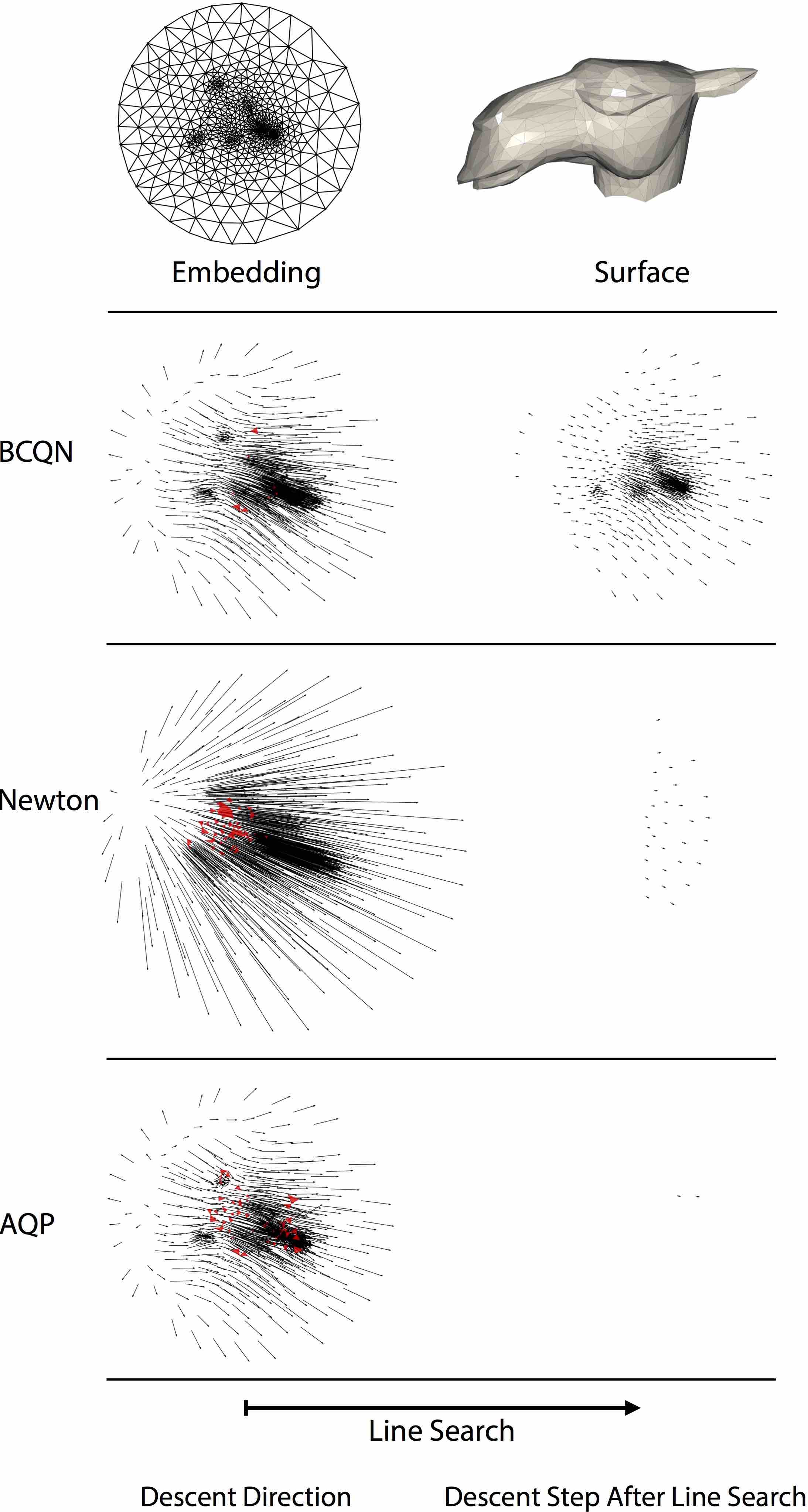
Figure 1: Line-search blocking. Barrier terms in nonconvex energies (here we use ISO) of the form $1/g(\sigma)$ can severely restrict step sizes in line searches even when expensive, high-quality methods such as Newton-type methods are applied. Left column: descent-direction vector fields, per vertex, in a descent step generated by BCQN, PN and AQP with potential blocking triangles rendered in red. Right, bottom rows: after line-search, close to collapsing elements have restricted the global step size for AQP and PN to effectively block progress. Right, top row: BCQN’s barrier-aware line-search filtering enables progress with significant descent directions.

Geometric Approximation methods specifically for geometry optimization have also been developed recently: SLIM [Rabinovich et al. 2016] and the AKAP preconditioner [Claici et al. 2017]. SLIM extends the local-global strategy to a wide range of distortion energies while AKAP applies an approximate Killing Vector Field operator as the proxy matrix. Both require re-assembly and factorization of their proxies for each iterate. SLIM and AKAP convergence are generally well improved over SGD and AQP [Rabinovich et al. 2016, Claici et al. 2017]. However, they do not match the convergence quality of the second-order, Newton-type methods, CM and PN [Shtengel et al. 2017]. SLIM falls well short of both CM and PN [Shtengel et al. 2017]. AKAP is more competitive than SLIM but remains generally slower to converge than PN in our testing, and is much slower than CM. At the same time SLIM and AKAP stencils, and so their fill-in, match CM’s and PN’s; see Figure 7. SLIM and AKAP thus require the same per-iteration compute cost and storage for linear solutions as PN and CM without the same degree of convergence benefit [Shtengel et al. 2017].

In summary, for smaller systems Newton-type methods have been, till now, our likely best choice for geometry optimization, while as we scale we have inevitably needed to move to first-order methods to remain tractable, while accepting reduced convergence rates and even the possibility of nonconvergence altogether. We develop a new quasi-Newton method, BCQN, that locally blends gradient information with the matrix Laplacian at each iterate to regain improved and robust convergence with efficient per-iterate storage and computation across scales while avoiding the current pitfalls of L-BFGS methods.

3.3 Line search

Once we have applied the effort to compute a search direction we would like to maximize its effectiveness by taking as large a step along it as possible. Because the energies we treat are nonlinear, too large a step size will actually make things worse by accidentally increasing energy. A wide range of line-search methods are thus employed that search along the step direction for sufficient decrease [Nocedal and Wright 2006]. However, when we seek to minimize nonconvex energies on meshes the situation is even tougher. Most (although not all) popular and important nonlinear energies, both in geometry processing and physics, are composed by the sum of rational fractions of singular values of the deformation gradient $W(F)=W(\sigma)=f(\sigma)/g(\sigma)$ where the denominator $g(\sigma)\rightarrow 0$ as $\sigma_{i}\rightarrow 0,\forall i\in[1,d]$. Notice that these $1/g(\sigma)$ barrier functions block element inversion. Irrespective of their source, these blocking nonconvex energies rapidly increase energy along any search direction that would collapse elements. To prevent this (and likewise the possibility of getting stuck in an inverted state) search directions are capped to prevent inversion of every element in the mesh. This is codified by Smith and Schaeffer’s Smith:2015:BPW line-search filter, applied before traditional line search, that computes the maximal step size that guarantees no inversions anywhere.

Unfortunately, this has some serious consequences for progress. Notice that if even a single element is close to inversion this can amputate the full descent step so much that almost no progress can be made at all; see Figure 1. This in many senses seems unfair as we should expect to be able to make progress in other regions where elements may be both far from inversion and yet also far from optimality. To address these barrier issues we develop an efficient barrier-aware filter that allows us to avoid blocking contributions from individual elements close to collapse while still taking large steps elsewhere in the mesh, see Figure 1, top.

3.4 Termination

Naturally we want to take as few iterates as possible while being sure that when we stop, we have arrived at an accurate solution according to some easily specified tolerance. The gold-standard in optimization is to iterate until the gradient is small $\|\nabla E\|<\epsilon$, for a specified tolerance $\epsilon>0$. This is robust as $\nabla E$ is zero only at stationary points, and with a bound on Hessian conditioning near the solution can even provide an estimate on the distance of $x$ to the solution.

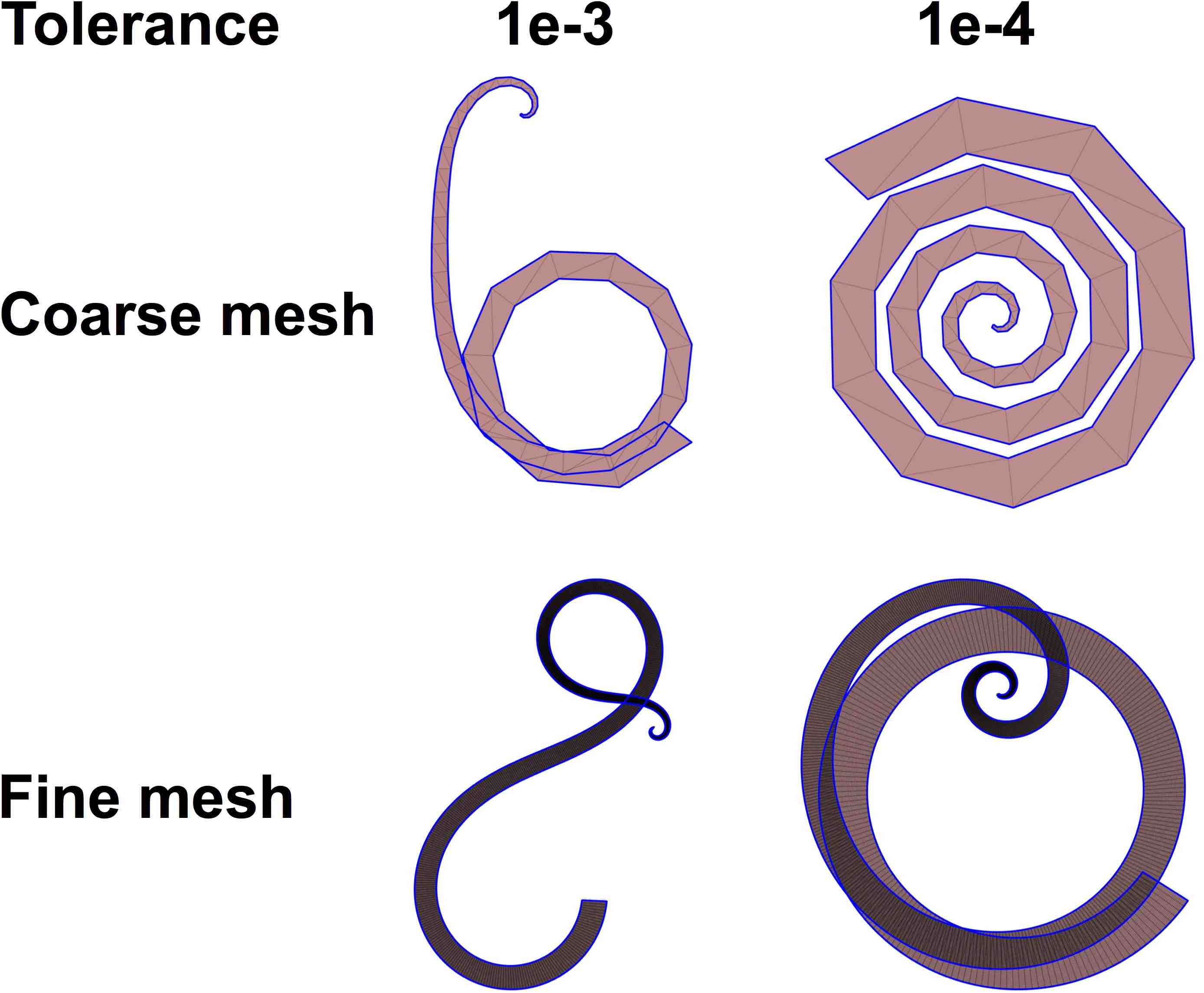
Figure 2: Standard termination measures, e.g. the vertex-scaled gradient norm above, are inconsistent across mesh, energy and scale changes.

However, an appropriate value of $\epsilon$ for a given application is highly depend on the mesh, its dimensions, degree of refinement, energy, etc. A common engineering rule of thumb to deal with refinement consistency is to instead divide the $L2$-norm of $\nabla E$ by the number of mesh vertices. However, as we see in the inset figure, this normalization does not help significantly, for example here across changes in mesh resolution for the 2D swirl test; see Section 8.2 for more experiments.

To avoid problem dependence, recent geometry optimization codes generally either take a fixed (small) number of iterations [Rabinovich et al. 2016] or iterate until an absolute or relative error in energy $\|E_{i+1}-E_{i}\|$ and/or position $\|x_{i+1}-x_{i}\|$ are small [Shtengel et al. 2017, Kovalsky et al. 2016]. However, experiments underscore there is not yet any method which always converges satisfactorily in the same fixed number of iterations, no matter varying boundary conditions, shape difficulty, mesh resolution, and choice of energy. Measuring the change in energy or position, absolutely or in relative terms, unfortunately cannot distinguish between an algorithm converging and simply stagnating in its progress far from the solution; again, there is not yet any method which can provably guarantee any degree of progress at every iterate before true convergence. Figure 3 illustrates, on the swirl example, how the reference AQP implementation declares convergence well before it reaches a satsifactory solution, when early on it hits a difficult configuration where it makes little local progress.

To provide reassuring termination criteria in practice and to enable fair comparisons of current and future geometry optimization problems we develop a gradient-based stopping criterion which remains consistent for optimization problems even as we vary scale, mesh resolution and energy type. This allows us, and future users, to set a default convergence tolerance in our solver once and leave it unchanged, independent of scale, mesh and energy. This likewise enables us to compare algorithms without the false positives given by non-converged algorithms that have halted due to lack of progress.

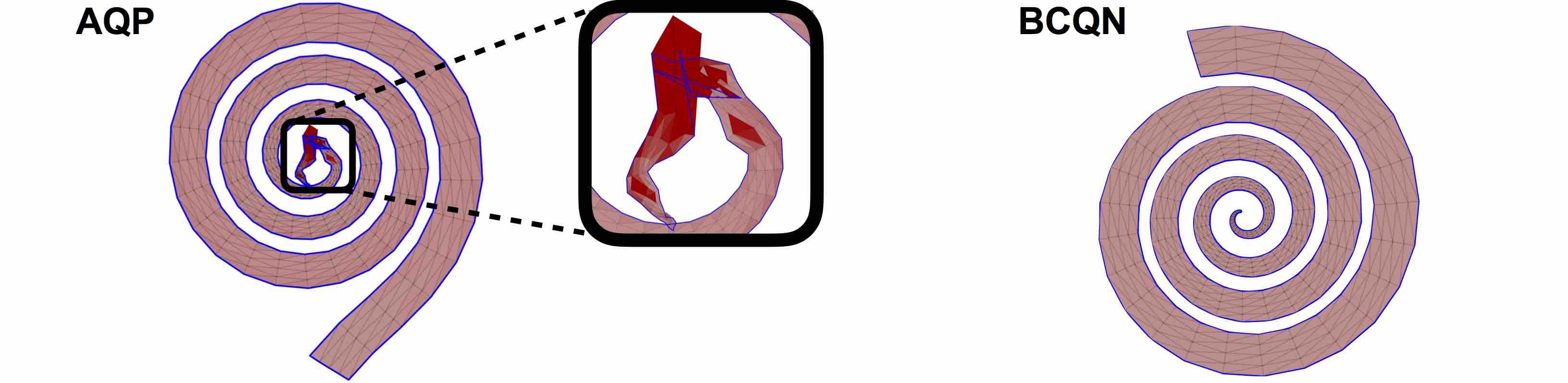
Figure 3: In the 2D swirl example, BCQN with our reliable termination criterion (right) only stops once it has actually reached a satsifactory solution. The reference AQP implementation (left) erroneously declares success early on when it finds two iterates have barely changed, but this is due only to hitting a difficult configuration where AQP struggles to make progress.

4 Blended Quasi-Newton

In this section we construct a new quadratic energy proxy which effectively blends the Sobolev gradient with L-BFGS-style updates to capture curvature information, avoiding the troubles previous quasi-Newton methods have encountered in geometry optimization. Apart from the aforementioned issue of a dense proxy incorrectly coupling distant vertices in L-BFGS and SL-BFGS, we also find that the gradients for non-convex energies with barriers can have highly disparate scales, causing further trouble for L-BFGS. The much smoother Sobolev gradient diffuses large entries from highly distorted elements to the neighborhood, giving a much better scaling. The Laplacian also provides essentially the correct structure for the proxy, only directly coupling neighboring elements in the mesh, and is well-behaved initially when far from the solution, thus we seek to stay close to the Sobolev gradient, as much as possible, while still capturing valuable curvature information from gradient history.

The standard (L-)BFGS approach exploits the secant approximation from the difference in successive gradients, $y_{i}=\nabla E(x_{i+1})-\nabla E(x_{i})$ compared to the difference in positions $s_{i}=x_{i+1}-x_{i}$,

$$\nabla^{2}E(x_{i+1})s_{i} \simeq y_{i}$$ (6)

$$\Rightarrow\quad\nabla^{2}E(x_{i+1})^{-1}y_{i} \simeq s_{i},$$

updating the current inverse proxy matrix $D_{i}$ (approximating $\nabla^{2}E^{-1}$ in some sense) so that $D_{i+1}y_{i}=s_{i}$. The BFGS quasi-Newton update is generically

$$\mathrm{QN}_{i}(z,D)=V_{i}(z)^{T}DV_{i}(z)+\frac{s_{i}s_{i}^{T}}{s_{i}^{T}z},\>\>V_{i}(z)=I-\tfrac{zs_{i}^{T}}{s_{i}^{T}z}.$$ (7)

We can understand this as using a projection matrix $V_{i}$ to annihilate the old $D$’s action on $z$, then adding a positive semi-definite symmetric rank-one matrix to enforce $\mathrm{QN}_{i}(z,D)z=s_{i}$. Classic BFGS uses $D_{i+1}=\mathrm{QN}_{i}(y_{i},D_{i})$, whereas L-BFGS uses

$$D_{i+1}=\mathrm{QN}_{i}(y_{i},\tilde{D}_{i}),$$ (8)

where $\tilde{D}_{i}$ has the oldest $\mathrm{QN}$ update removed, and crucially represents each $D$ as a product of linear operators, rather than an explicit full matrix. Only the last $m$ $\{s,y\}$ vector pairs (we use $m=5$) along with the initial $D_{1}$ (we use the inverse Laplacian, storing only its Cholesky factor) are stored; application of $D$ is then just a few vector dot-products and updates along with backsolves for the Laplacian.

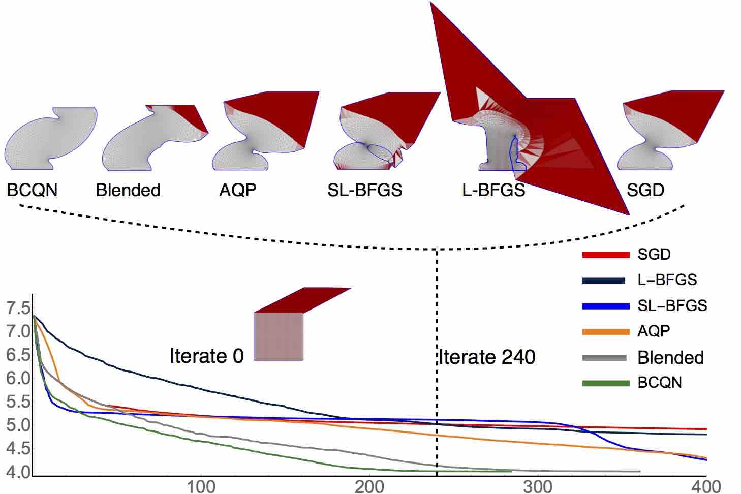
Figure 4: A 2D shearing deformation stress test with MIPS energy, comparing methods by plotting iteration vs. energy. Both L-BFGS as well as inverse Laplacian initialized (SL-BFGS) have slow convergence as previously reported – especially when compared to SGD and AQP which use just the Laplacian. At iteration 240 the visualized deformations show both L-BFGS-based methods suffering from swelling due to inaccurate coupling of distant elements. Applying our blending model alone (Blended) is highly effective, while our full BCQN method gives the best results overall.

4.1 Greedy Laplacian Blending

Experiments show that far from the solution, the Laplacian is often a much more effective proxy than the L-BFGS secant version: see AQP/SGD vs. L-BFGS in Figure 4. In particular, the difference in energies $y$ may introduce spurious coupling or have badly scaled entries near distorted triangles. In this case if the energy were based on the Laplacian itself (the Dirichlet energy), the difference in gradients would be the better behaved $Ls$. This motivates trying the update with $Ls$ instead of $y$,

$$D_{i+1}=\mathrm{QN}_{i}(Ls_{i},\tilde{D}_{i}),$$ (9)

which will keep us consistent with Sobolev preconditioning, which is very effective in initial iterations. However, to achieve the superlinear convergence L-BFGS offers, near the solution we will want to come closer to satsifying the secant equation, switching to using $y$ instead.

We can thus imagine a blending strategy, which uses

$$z_{i}=(1-\beta_{i})y_{i}+\beta_{i}Ls_{i}$$ (10)

in $\mathrm{QN}(z_{i},\tilde{D}_{i})$, with blending parameter $\beta_{i}\in[0,1]$. A greedy strategy might choose $\beta_{i}$ to scale $Ls_{i}$ to be as close to $y_{i}$ as possible,

$$\beta_{i}=\mathop{\rm argmin}_{\beta\in[0,1]}\|y_{i}-\beta Ls_{i}\|^{2},$$ (11)

in other words using the projection of $y_{i}$ onto $Ls_{i}$. This comes as close as possible to satsifying the secant equation with $Ls_{i}$, then makes up the rest with $y_{i}$. Solving (11) gives

$$\beta_{i}=\mathrm{proj}_{[0,1]}\left(\frac{{y_{i}}^{T}Ls_{i}}{\|Ls_{i}\|^{2}}\right).$$ (12)

Observe that when $Ls$ is roughly aligned with the gradient jump $y$ , but $y$ is as large or larger, $\beta$ grows and Laplacian smoothing increases — as we might hope for initially when far from the solution, where the Sobolev gradient is most effective. When the energy Hessian diverges strongly from from the Laplacian approximation, perhaps when the cross-terms between coordinates missing from the scalar Laplacian are important, then $\beta$ will decrease, so that contributions from $y_{i}$ again grow. Finally, as the gradient magnitudes decreases close to the solution, $\beta$ will similarly decay, ideally regaining the superlinear convergence of L-BFGS near local minima.

4.2 Blended Quasi-Newton

With the blending projection (12) in place we experimented with a range of rescalings in hopes of further improving efficiency and robustness. After extensive testing we have so far found the following scaling to offer the best performance:

$$\begin{split}\beta_{i}=\mathrm{proj}_{[0,1]}\Big{(}\frac{\mathrm{normest}(L){y_{i}}^{T}Ls_{i}}{A(V,T)}\Big{)},\\ \text{with}\>\>A(V,T)=\Big{(}\sum_{t\in T}a_{t}\Big{)}^{\frac{2(d-1)}{d}}.\end{split}$$ (13)

Here $\mathrm{normest}(L)$ is an efficient estimate of the matrix 2-norm using power iteration, and $A(V,T)$ is a constant normalizing term with appropriate dimensions and so no longer has the same potential concern for sensitivity in the denominator when $Ls$ is small but $s$ isn’t. Both terms are computed just once before iterations begin and reused throughout.

As mentioned, we initialize the inverse proxy with $D_{1}=L^{-1}$, thus starting with Laplacian preconditioning. With line search satisfying Wolfe confitions our proxy remains SPD across all steps [Nocedal and Wright 2006]. Each step jointly updates $D_{i}$ using the standard two-loop recursion and finds the next descent direction $s_{i}=-D_{i}\nabla E(x_{i})$. Figure 4 illustrates the gains possible from blended quasi-Newton compared to both standard L-BFGS and Sobolev gradient algorithms, while then applying our barrier-aware filter, derived in our next section gives best results with our full BCQN algorithm.

5 Barrier-Aware Line Search Filtering

As mentioned in Section 3.3 and shown in Figure 1, the barrier factor $1/g(\sigma)$ in nonconvex energies typically dominates step size in line search. Even a single element that is brought close to collapse by the descent direction, $p_{i}$, can restrict the line search step size severely. The computed step size $\alpha_{i}$ then scales $p_{i}$ globally so that all elements, not just those that are going to collapse along $p_{i}$, are prevented from making progress. To avoid this, a natural strategy suggests itself: when the descent direction would cause elements to degenerate towards collapse along the full step, rather than simply truncating line search as in Smith and Schaefer Smith:2015:BPW, we filter collapsing contributions from the search direction prior to line search. We call this strategy barrier-aware line search filtering.

5.1 Curing line search

Figure 5: Direct filtering does not work. Zeroing out inverting components of descent directions or gradients makes the search direction inconsistent with the objective and so prevents convergence, leading to termination at poor solutions (a) and (b). Left: we initialize a 2D shear deformation, constraining the top of a bar to slide rightwards. Middle: direct filtering of the descent direction (a) and the gradient (b) allow large descent steps forward unblocked from the contributions of close-to-collapsed elements. However, this results in termination at shapes that that do not satisfy optimality of the original minimization. Right: compare to an optimal solution for this problem (c) obtained with BCQN.

Figure 5 illustrates how the simplest possible filters, zeroing out contributions from nearly-inverted elements in either the search direction (5a) or the gradient before Laplacian smoothing (5b) fail. We must be able to make progress in nearly-inverted elements when the search direction can help, or there is no hope for reaching the actual solution; simple zeroing fails to converge, which is no surprise as it in essence is arbitrarily manipulating the target energy, changing the problem being solved. We instead want to augment the original optimization problem in a way which doesn’t change the solution, but gives us a tool to safely deal with problem elements so the search direction $p_{i}$ doesn’t cause them to invert, ideally with a small fixed cost per iteration.

5.2 One-Sided Barriers in Geometry Optimization

Element $t\in T$ is inverted at positions $x$ precisely when the orientation function $a_{t}(x)=\det(F_{t}(x))$ is negative. Concatenating over $T$, the global vector-valued function for element orientations is then

$$a(\cdot)=\big{(}a_{1}(\cdot),...,a_{m}(\cdot)\big{)}^{T}.$$ (14)

As long as $a(x)>0$, no element is collapsed or inverted, and the energy remains finite. Note, however, many energies are also finite for inverted elements $a_{t}(x)<0$, only blowing up at collapse $a_{t}(x)=0$, so technically there may exist local minima where $\nabla E(x^{*})=0$ yet some elements are inverted. Generally, practitioners wish to rule these potential solutions out however, with two implicit but so far informal assumptions of locality: the initial guess is not inverted, $a(x_{1})>0$, and that the solver follows a path which never jumps through the barrier to inversion.

We formalize these requirements in the optimization as

$$\mathop{\rm min}_{x}\{E(x)\ :\ a(x)\geq 0\}.$$ (15)

Adding the constraint $a(x)\geq 0$ now explicitly restricts our optimization to noninverting deformations but otherwise leaves the desired solution unchanged. (See Supplement, Section 1, for proof.)

5.3 Iterating Away from Collapse

With problem statement (15) in place, we now exploit it in curing the search direction from collapsing elements. At each iterate $i$, form the projection

$$\mathop{\rm min}_{p}\left\{\|p+D_{i}\nabla E(x_{i})\|_{2}^{2}\>:\>a(x_{i})+\nabla a(x_{i})^{T}p\geq 0\right\}$$ (16)

of the predicted descent direction $\tilde{p}_{i}=-D_{i}\nabla E(x_{i})$ onto the subset satisfying a linearization of the no-collapse condition. Satisfying (16) exactly would ensure that projected directions would not locally generate collapse and likewise preserve symmetry [Smith et al. 2012]. However, its exact solution is neither necessary nor efficient. Instead, we construct an approximate solution to (16) as a filter that helps avoid collapse, preserves symmetry, and guarantees a low cost for computation for all descent steps.

Strict convexity of the projection guarantees that a minimizer $p^{*}$ of (16) is given by the KKT conditions [Bertsekas 2016]

$$p^{*}+D_{i}\nabla E(x_{i})-\nabla a(x_{i})\lambda^{*}=0,$$ (17)

$$0\leq\lambda^{*}\perp a(x_{i})+\nabla a(x_{i})^{T}p^{*}\geq 0.$$ (18)

We simplify with $C_{i}=\nabla a(x_{i})$, $M_{i}=\nabla a(x_{i})^{T}\nabla a(x_{i})$, and $b_{i}=a(x_{i})$, then form the Schur complement of the above to arrive at an equivalent Linear Complementarity Problem (LCP) [Cottle et al. 2009]

$$\begin{split}0\leq\lambda^{*}\perp M_{i}\lambda^{*}+C_{i}^{T}p_{i}+b_{i}\geq 0,\end{split}$$ (19)

and then a damped Jacobi splitting with $M_{i}=\omega^{-1}T_{i}+(M_{i}-\omega^{-1}T_{i})$, diagonal $T_{i}=\mathrm{diag}(M_{i})$ and damping parameter $\omega\in(0,1)$. This gives us an iterated LCP ranging over iteration superscripts $j$,

$$\begin{split}0\leq\lambda^{j+1}\perp\omega^{-1}T_{i}\lambda^{j+1}+M_{i}\lambda^{j}-\omega^{-1}T_{i}\lambda^{j}+C_{i}^{T}p_{i}+b_{i}\geq 0.\end{split}$$ (20)

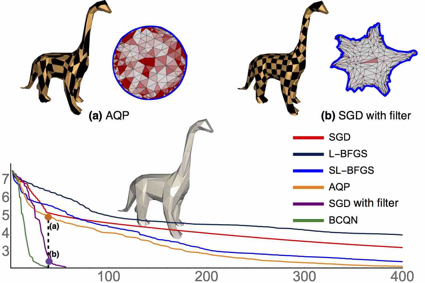
Figure 6: Line search filtering. Bottom: We optimize a uv-parameterization with the MIPS energy to consider line search filtering behavior, plotting energy (y-axis) against iteration counts for a range of methods. Just adding our barrier-aware line search filtering alone to SGD improves its convergence by well over an order of magnitude, and almost an order of magnitude over AQP as well as plain L-BFGS and SL-BFGS. BCQN with blending and line search filtering improves convergence even further. Top: a comparison of the embeddings and texture-maps for AQP and SGD with the filter at the $40^{\textrm{th}}$ iterate.

5.4 Line Search Filtering

Each iteration of the splitting (20) simplifies to the damped projected Jacobi (DPJ) update

$$\lambda^{j+1}\leftarrow\left[\lambda^{j}-\omega T^{-1}\big{(}C_{i}^{T}(C_{i}\lambda^{j})+c_{i}\big{)}\right]^{+},$$ (21)

with constant $c_{i}=C_{i}^{T}p_{i}+b_{i}$. Here each of the $m$ entries in $\lambda^{j+1}$ can be updated in parallel (unlike with Gauss-Seidel iteration). As $M_{i}$ is PSD this iteration process converges to (19) [Cottle et al. 2009] and so to (16). We do not seek a tight solution, however, as we just want to be sure the worst blocks to line search are filtered away. Therefore we initialize with $\lambda^{0}=0$ to avoid unnecessary perturbation, use a coarse termination tolerance for DPJ (see below), and never use more than a maximum of 20 DPJ iterations.

At each DPJ iteration $j$ we check for termination with an LCP specialized measure, the Fischer-Burmeister function [Fischer 1992] $\mathrm{FB}(\lambda^{j},M_{i}\lambda^{j}+c_{i})$ evaluated as

$$\mathrm{FB}(a,b)=\sqrt{\sum_{k\in[1,m]}\left(a_{k}+b_{k}-\sqrt{a_{k}^{2}+b_{k}^{2}}\right)^{2}}.$$ (22)

As we initialize with $\lambda^{0}=0$, when $p_{i}$ is non-collapsing $\mathrm{FB}=0$, and thus no line search filtering iterations will be applied. Likewise, we stop iterations whenever the $\mathrm{FB}$ measure is roughly satisfied by either a relative error of $<10^{-3}$ or an absolute error $<10^{-6}$.

Filtering thus applies a fixed maximum upper limit on computation and performs no iterations when not necessary. Upon termination of DPJ iterations, plugging our final $\lambda$ into (17) we obtain our update to form the line search filtered descent direction

$$p^{\ell}_{i}=p_{i}+C_{i}\lambda.$$ (23)

As Figure 1 shows, despite the rough nature of the filter, it can make a dramatic difference in line search.

6 Termination Criteria

Every iterative method for minimizing an objective function $E(x)$ must incorporate stopping criteria: when should an approximate solution be considered good enough to stop and claim success? Clearly, in the usual case where the actual minimum value of $E(x)$ is unknown, basing the test on the current value of $E(x_{i})$ is futile. As noted in Section 3.4, stopping when successive iterates are closer than some tolerance is vulnerable to false positives (halting far from a solution), as is using a fixed number of iterations. Although monitoring $\|\nabla E\|$ is robust, each individual problem may need a different tolerance to define a satisfactory solution even when normalized by number of vertices: see Figures 2 and 10. We thus propose a new way to derive and construct an appropriate, roughly problem-independent, relative scale for a gradient-based measure for a stopping criterion.

6.1 Characteristic Gradient Norm

All energies we consider are summations of per-element energy densities $W(\cdot)$ computed from the deformation gradient $F_{t}(x)$ and weights $a_{t}$, in each element $t$, as per equation (2). To simplify the following we can then evaluate energy densities on the vectorized deformation gradient as $W\big{(}vec(F_{t})\big{)}=W(G_{t}x)$, where $G_{t}$ is the linear gradient operator for element $t$. The full energy gradient is then

$$\nabla E(x)=\sum_{t\in T}a_{t}G_{t}^{T}\nabla W(G_{t}x).$$ (24)

We wish to generate a “characteristic” value we can compare this gradient to meaningfully, with the same dimensions; we will do this with each component of the above summation separately.

First observe that the deformation gradient, $F_{t}$, the argument to $W$, is dimensionless and therefore $\nabla W$ has the same dimensions as $W$, and even as the element Hessian $\nabla^{2}W$. For the simplest quadratic energy densities, this Hessian has the attractive property of being constant; we thus choose to use the 2-norm of the Hessian, evaluated about the deformation gradient at rest ($F_{t}=I$), to get a representative value for $\nabla W$:

$$\langle W\rangle=\|\nabla^{2}W(I)\|_{2}.$$ (25)

Second, note that the $i^{\textrm{th}}$ part of $G_{t}$ for a triangle (respectively tetrahedra) $t$ containing vertex $i$ will attain its maximum value for fields which are constant along the opposing edge (triangle) and that value will be the reciprocal of the altitude. Up to a factor of $2$ ($3$), this is the length (area) of the opposing edge (triangle) divided by the rest area (volume), of the element, i.e. $a_{t}$. Summing over all incident elements, weighted by $a_{t}$, we arrive at a characteristic value for vertex $i$ of $\ell_{i}$ equalling the perimeter (surface) area of the one-ring of vertex $i$. We compute this value for all vertices, giving us the vector $\ell(V,T)=(\ell_{1},...,\ell_{n})^{T}\in\mathbb{R}^{n}$, with one scalar entry per vertex.

The product of our energy and mesh values together form the characteristic value for the norm of the gradient

$$\langle W\rangle\|\ell(V,T)\|,$$ (26)

where we take the same vector norm as that with which we evaluate $\|\nabla E(x)\|$; we use the 2-norm in all our experiments. For all methods we stop iterating when

$$\|\nabla E(x)\|\leq\epsilon\langle W\rangle\|\ell(V,T)\|,$$ (27)

given a dimensionless tolerance $\epsilon$ from the user, which is now essentially mesh- and energy-independent. See Figures 2, 9 and 10 as well as our experimental analysis in Section 8 for evaluation.

7 The BCQN Algorthim

Given: $x_{1}$, $E$, $\epsilon$    

Initialize and Precompute:

          $s=\epsilon\langle W\rangle\|\ell(V,T)\|$     // Characteristic termination value (§6)

          $L,\>\>D\leftarrow L^{-1}$     // Initialize blend model (§4)

          $g_{1}=\nabla E(x_{1}),\>\>i=1$

while $\|g_{i}\|>s$ do   // Termination criteria (§6)

    $p\leftarrow-Dg_{i}$    // Precondition gradient (§4)

    // Assemble for DPJ iterations (§5):

       $C\leftarrow\nabla a(x_{i})$

       $M\leftarrow C^{T}C,\>\>c\leftarrow C^{T}p+a(x_{i})$

       $E\leftarrow\mathrm{diag}(M)^{-1},\>\>\lambda\leftarrow 0$

    $\mathit{fb}\leftarrow\textrm{FB}(\lambda,M\lambda+c)$    // LCP residual (Equation (22) in §5)

    for $j=1$ to 20    // Line-search preconditioning (§5)

      if $\mathit{fb}<10^{-6}$ then   break    end if

      $\mathit{fb}\leftarrow\mathit{fb}_{\mathrm{next}}$

       $\lambda\leftarrow[\lambda-\tfrac{1}{2}E\big{(}C^{T}(C\lambda)+c\big{)}]^{+}$ // Parallel project (§5)

      $\mathit{fb}_{\mathrm{next}}\leftarrow\textrm{FB}(\lambda,M\lambda+c)$

      if $|\mathit{fb}-\mathit{fb}_{\mathrm{next}}|/\mathit{fb}<10^{-3}$ then   break    end if

   end for

    $p^{\ell}\leftarrow p+C\lambda$    // Line-search filtered search direction (§5)

   $\alpha\leftarrow\text{LineSearch}(x_{i},p^{\ell},E)$     // Line search (§4)

   $x_{i+1}=x_{i}+\alpha p^{\ell}$     // Descent step (§4)

    $g_{i+1}=\nabla E(x_{i+1})$

   $D\leftarrow\text{Blend}(D,L,x_{i+1},x_{i},g_{i+1},g_{i})$   // BCQN blending update (§4)

   $i\leftarrow i+1$

end while

ALGORITHM 1 Blended Cured Quasi-Newton (BCQN)

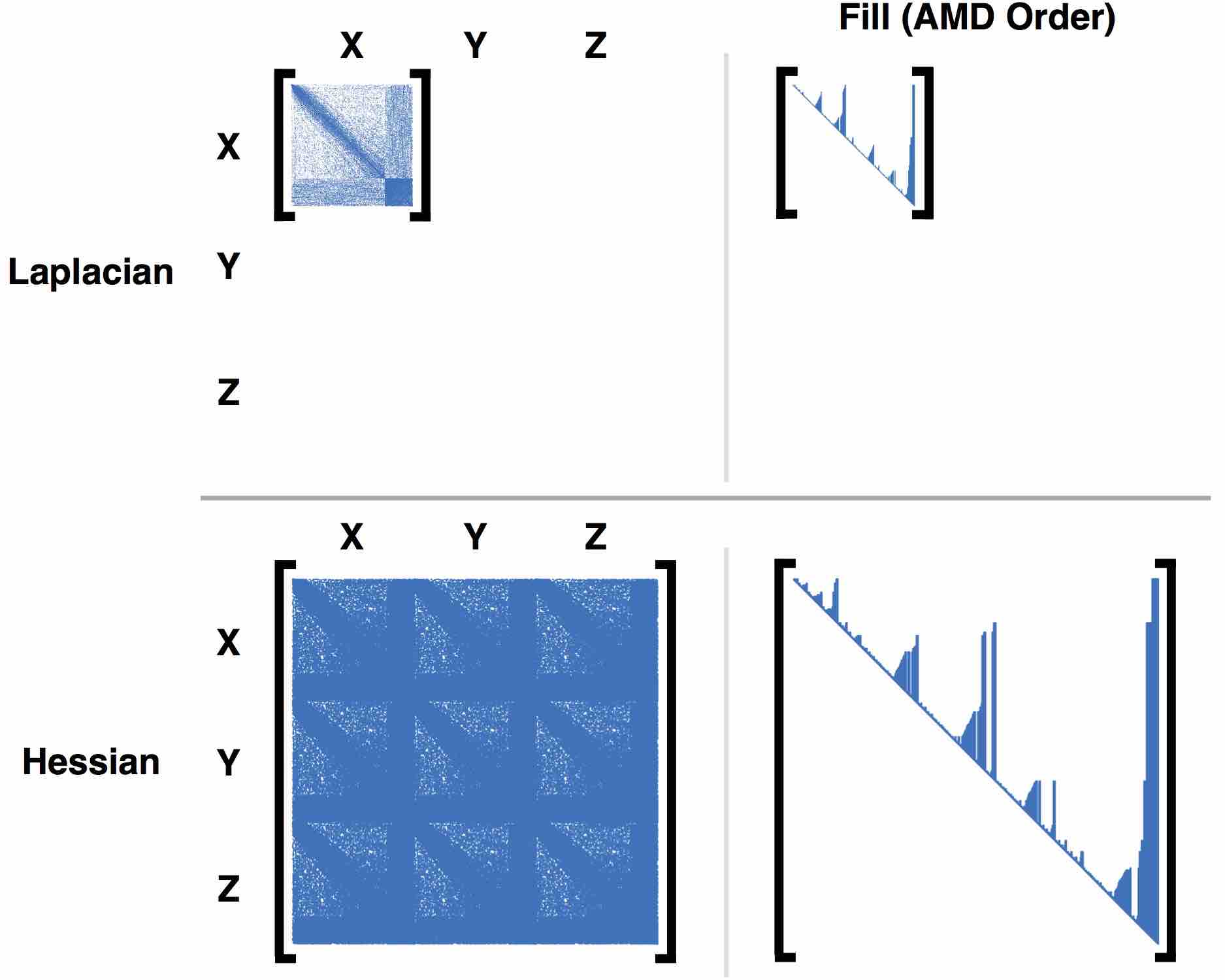
Figure 7: Sparsity Differences in Proxies. Left: The scalar Laplacian (top) is smaller and sparser than the Hessian and its approximations (bottom) used in CM, PN, SLIM and AKAP. Right: This results in a much cheaper factorization and solve for the Laplacian; it is applied in both BCQN and AQP independently to each coordinate.

Algorithm 1 contains our full BCQN algorithm in pseudocode. The dominant cost, for both memory and runtime, is the Laplacian solve embedded in the application of $D$, which again is not stored as a single matrix, but rather is a linear transformation involving a few sparse triangular solves with the Laplacian’s Cholesky factor and outer-product updates with a small fixed number of L-BFGS history vectors. Recall that we separately solve for each coordinate with a scalar Laplacian, not using a larger vector Laplacian on all coordinates simultaneously; this also exposes some trivial parallelism. Apart from the Laplacian, all steps are either linear (dot-products, vector updates, gradient evaluations, etc.) or typically sublinear (DJP assembly and iterations, which only operate on the small number of collapsing triangles, and again are easily parallelized).

As Lipton et al. proved lipton:1979:gnd, the lower bounds for Cholesky factorization on a two-dimensional mesh problem with $n$ degrees of freedom are $O(n\log n)$ space and $O(n^{3/2})$ sequential time, and in three-dimensional problems where vertex separators are at least $O(n^{2/3})$, their Theorem 10 shows the lower bounds are $O(n^{4/3})$ space and $O(n^{2})$ sequential time. On moderate size problems running on current computers, the cost to transfer memory tends to dominate arithmetic, so the space bound is more critical until very large problem sizes are reached.

7.1 Comparison with Other Algorithms

The per-iterate performance profile of AQP is most similar to BCQN: it too is dominated by a Laplacian solve. The only difference is the extra linear and sublinear work which BCQN does for the quasi-Newton update and the barrier-aware filtering; even on small problems, this overhead is usually well under half the time BCQN spends, and as the next section will show, the improved convergence properties of BCQN render it faster.

The second-order methods we compare against, PN and CM, as well as the more approximate proxy methods, SLIM and AKAP, all use a fuller stencil which couples coordinates. The same asymptotics for Cholesky apply, but whereas AQP and BCQN can solve a scalar $n\times n$ Laplacian $d$ times (once for each coordinate, independently), these other methods must solve a single denser $nd\times nd$ matrix, with $d^{2}$ times more nonzeros: see Figure 7. Moreover, the matrix changes at each iteration and must be refactored, adding substantially to the cost: factorization is significantly slower than backsolves.

8 Evaluation

8.1 Implementation

We implemented a common test-harness code to enable the consistent evaluation of the comparitive performance and convergence behavior of SGD, PN, CM, AQP, L-BFGS and BCQN across a range of energies and geometry optimization tasks including parameterization as well as 2D and 3D deformations, where these methods allow. For AQP this extends the number of energies it can be tested with, while more generally providing a consistent environment for evaluating all methods. We hope that this code will also help support the future evaluation and development of new methods for geometry optimization.

The main body of the test code is in MATLAB to support rapid prototyping. All linear system solves are performed with MATLAB’s native calls to SuiteSparse [Chen et al. 2008] with additional computational-heavy modules, primarily common energy, gradient and iterative LCP evaluations, implemented in C++. As linear solves are the bottleneck in all methods covered here, an additional speed-up to all methods is possible with Pardiso [Petra et al. 2014b, Petra et al. 2014a] in place of SuiteSparse; however, as discussed in Section 8.4 this does not change the relative merits of the methods, and would add an additional external dependency to the test code. For verification we also confirm that iterations in the test-harness AQP and CM implementations match the official AQP [Kovalsky et al. 2016] and CM [Shtengel et al. 2017] codes.

All experiments were timed on a four-core Intel 3.50GHz CPU. We have parallelized the damped Jacobi LCP iterations with Intel TBB; with more cores the overhead reported below for LCP iterations is expected to diminish rapidly. For all UV parameterization problems we compute initial locally injective embeddings via the initialization code from Kovalsky et al. Kovalsky:2016:AQP. On rare occasions this code fails to find a locally injective map, so we then revert to a Tutte embedding as a failsafe using the initialization code from Rabinovich et al. Rabinovich:2016:SLI. To enforce Dirichlet boundary conditions, i.e. positional constraints, we use a standard subspace projection [Nocedal and Wright 2006], i.e. removing those degrees of freedom from the problem. When line search is employed we first find a maximal non-inverting step size with Smith and Schaefer’s method Smith:2015:BPW, followed by standard line search with Armijo and curvature conditions.

8.2 Termination

To evaluate termination criteria behavior we first instrumented two geometry optimization stress-test examples: the Swirl deformation [Chen et al. 2013] and the Hilbert curve UV parametrization [Smith and Schaefer 2015]. We run both examples to convergence ($10^{-6}$ using our characteristic gradient) reaching the final target shapes for each. Within these optimizations we record the 2-norm of gradient, the vertex-normalized 2-norm of gradient, the relative error measure [Kovalsky et al. 2016, Shtengel et al. 2017] and our characteristic gradient norm for all iterations.

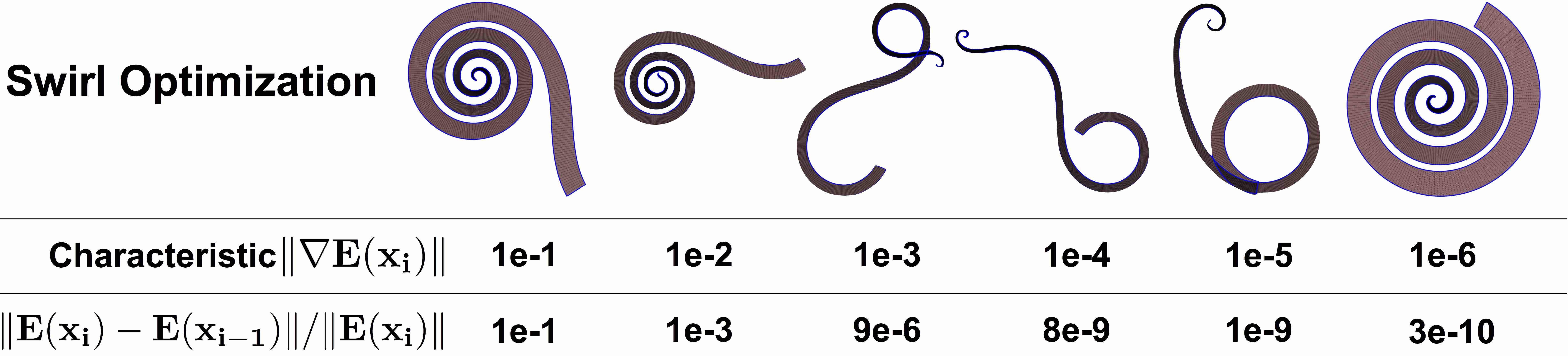
Figure 8: Termination criteria comparison. Left to right: We find key points in the sequential progress of the optimized mesh in the Swirl optimization (ISO energy) example at regular intervals of $10\times$ decrease in our characteristic norm. We compare with the relative error measures at these same points.

Figure 8 shows the Swirl mesh obtained during BCQN iteration at regular intervals of $10\times$ decrease in our characteristic norm. Observe that they correspond to natural points of progress; see our supplemental video of the entire optimization sequence for reference. For comparison we also provide the corresponding relative error measures, which varies much less steadily.

In Figure 9 we compare termination criteria more closely for a UV parametrization problem, the Hilbert curve example. We plot our characteristic gradient norm (blue) and the relative energy error [Kovalsky et al. 2016, Shtengel et al. 2017] (orange) as BCQN proceeds. Note that the characteristic gradient norm provides consistent decrease corresponding to improved shapes and so provides a practical measure of improvement. The local error in energy, on the other hand, varies greatly, making it impossible to judge how much global progress has been made towards the optimum.

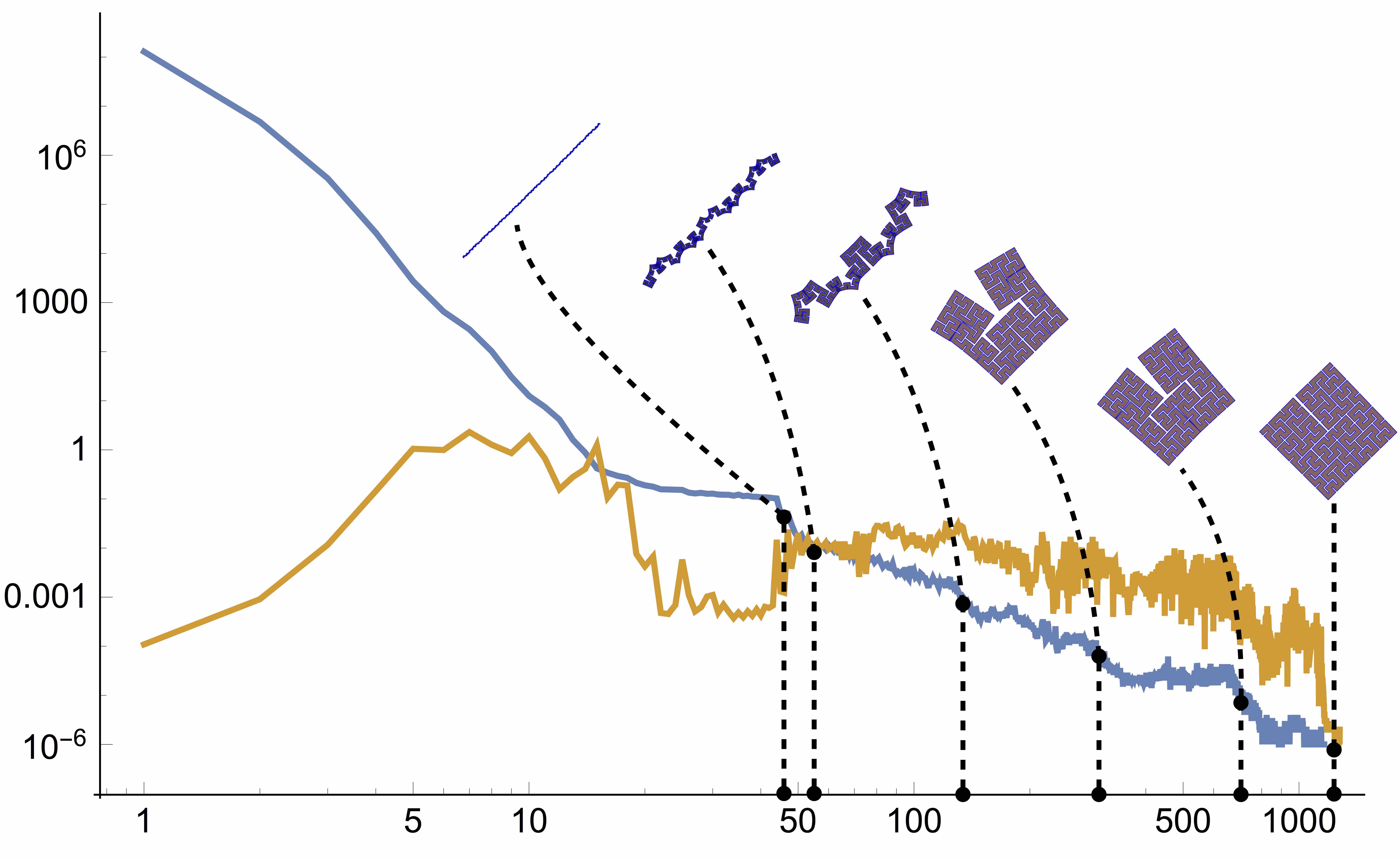
Figure 9: Measuring improvement. Solving a UV parametrization of the Hilbert curve with BCQN, we plot our characteristic gradient norm in blue and the relative energy error in orange as the method proceeds, on a logarithmic scale. Iterates are shown at decreases in the characteristic gradient norm by factors of 10, illustrating its efficacy as a global measure of progress, while the relative energy error measures only local changes with little overall trend.

Figure 10 illustrates consistency across changing tolerance values, mesh resolutions, and scales. example. We show the iterates at measures $10^{-3}$, $10^{-4}$and $10^{-5}$ for both our characteristic gradient norm and the raw gradient norm, for meshes with varying refinement and varying dimension (rescaling coordinates by a large factor). Similar to Figure 2 comparing the vertex-normalized gradient norm, there are large disparities for the raw gradient norm, but our characteristic gradient norm is consistent.

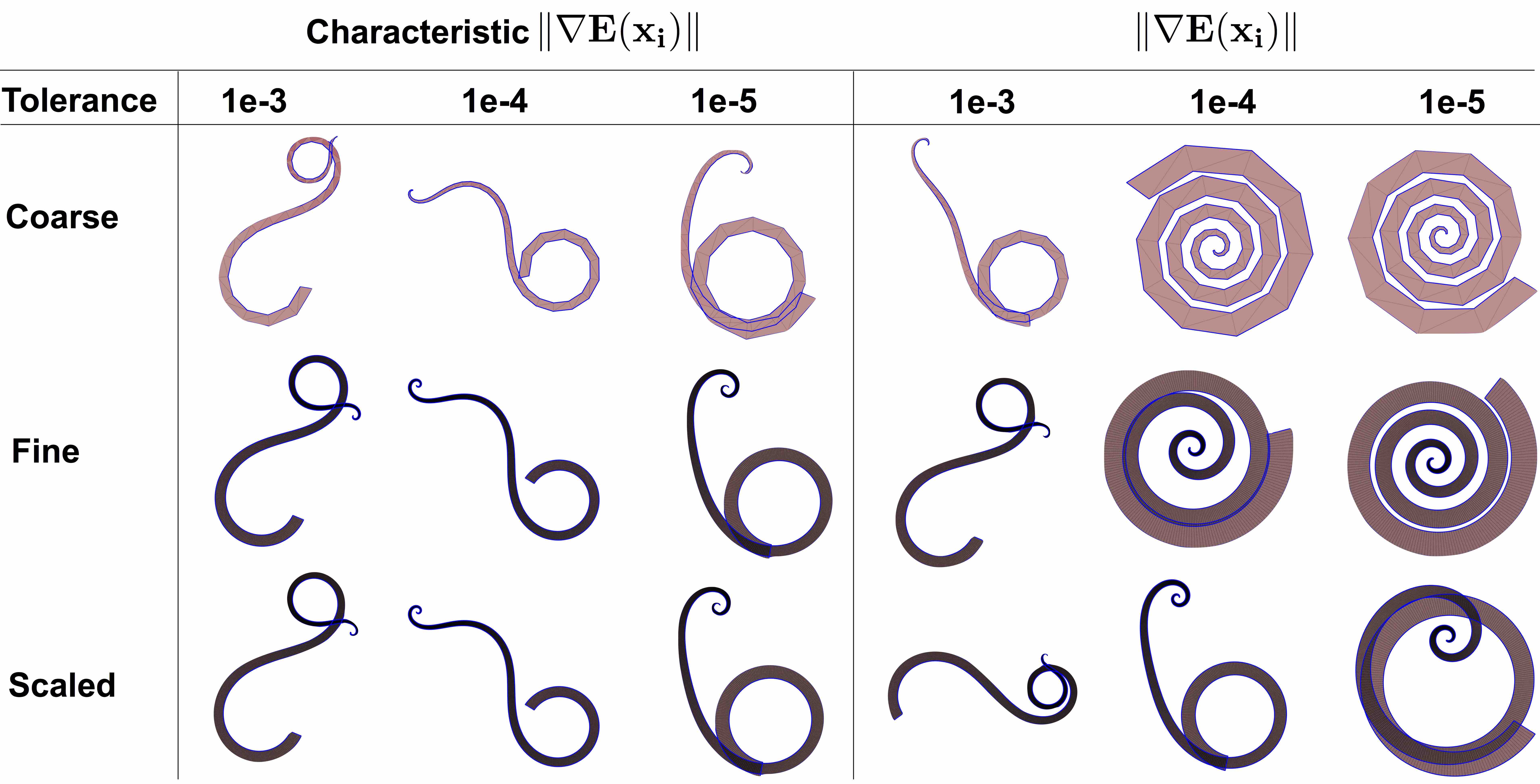
Figure 10: Termination criteria comparison across mesh refinement and scale. Left and right: we show the Swirl optimization when our characteristic norm (left) and the standard gradient norm (right) reach $10^{-3},10^{-4}$ and $10^{-5}$. Top to bottom: the rows show optimization with a coarse mesh, a fine mesh, and the same fine mesh uniformly scaled in dimension by $100\times$. Note the consistency across mesh resolution and scaling for our characteristic norm and the disparity across the standard gradient norm.

Tolerances

The Swirl and Hilbert curve examples are both extreme stress tests that require passing through low curvature regions to transition from unfolding to folding; see e.g., Figure 8 above and our videos. For these extreme tests we used a tolerance of $10^{-6}$ for our characteristic gradient norm to consistently reach the final target shape. However, for most practical geometry optimization tasks such a tolerance is excessively precise. In experiments across a wide range of energies and UV parametrization, 2D and 3D deformation tasks, including those detailed below, we found that $\|\nabla E(x)\|\leq 10^{-3}\langle W\rangle\|\ell(V,T)\|$ consistently obtained good-looking solutions with essentially no further visible (or energy value) improvement possible. We argue this is a sensible default except in pathological examples. For all examples discussed here and below, with the exception of the Swirl and the Hilbert curve tests, we thus use $\epsilon=10^{-3}$ for testing termination.

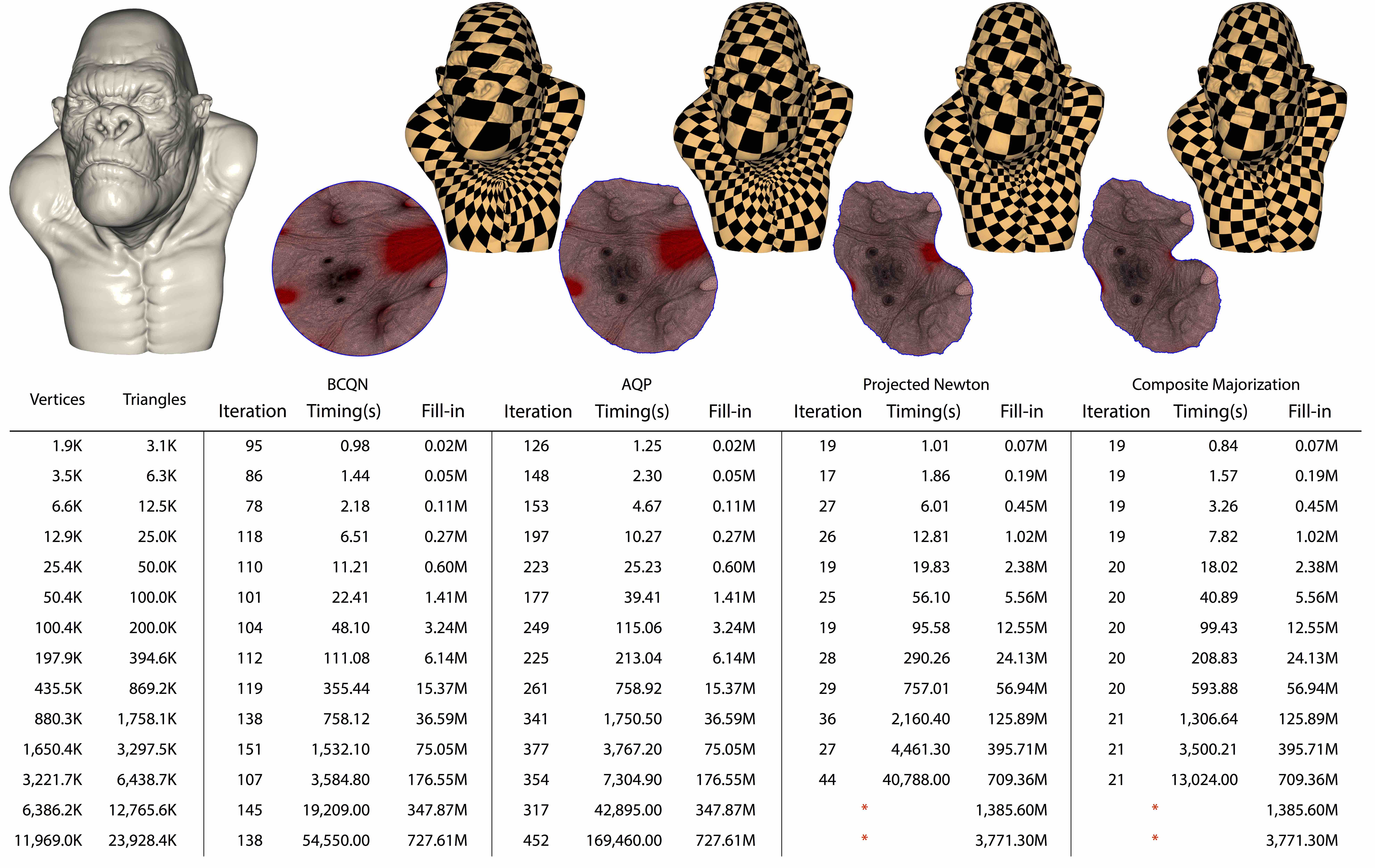
Figure 11: UV Parameterization Scaling, Timing and Sparsity. Performance statistics and memory use for increasing mesh sizes up to 23.9M triangles, comparing BCQN with AQP, PN and CM. For the Gorilla UV parametrization with ISO energy we repeatedly double the mesh resolution and, for each method, report number of iterations to convergence (characteristic norm $<10^{-3}$), wall-clock time (seconds) to convergence, and the nonzero fill-in for the linear systems solved by each method. We use * to indicate out-of-memory failure for matrix factorization; see §8 for discussion. Also note that stencils for CM and PN are identical (differing only by actual entries) while AQP and BCQN both solve with the same smaller scalar Laplacian.

8.3 Newton-type methods

While Newton’s method, on its own, handles convex energies like ARAP well [Chao et al. 2010] it is insufficient for nonconvex energies: modification of the Hessian is required [Shtengel et al. 2017, Nocedal and Wright 2006]. Here we examine the convergence, performance and scalability of Projected Newton (PN) [Teran et al. 2005], a general-purpose modification for nonconvex energies, and CM [Shtengel et al. 2017], a more recent convex majorizer currently restricted to 2D problems and a trio of energies (ISO, Symmetric ARAP and NH), and compare them with AQP and BCQN. For the 2D parameterization problems in Figure 11 we can compare all four methods while for the 3D deformation problems in Figures 12 and 13 CM is not applicable.

As we increase the size of the 2D problem by mesh refinement in Figure 11, both CM and PN maintain low and almost constant iteration counts to converge, with CM enjoying an advantage for larger problems; in Figure 12

Figures 11, 12, and 13 examine the scaling behavior of the various methods under mesh refinement, for 2D parameterization and 3D deformation. The Newton-type methods PN and CM (when applicable) maintain low iteration counts that only grow slowly with increasing mesh size; from the outset BCQN and AQP require more iterations, though the iteration count also grows slowly for BCQN. Nonetheless, BCQN is the fastest across all scales in each test as its overall cost per iteration remains much lower. BCQN iterations require no re-factorizations (which scales poorly, particularly in 3D, as discussed in Section 7) and only solves smaller and sparser scalar Laplacian problems per coordinate compared to the larger and denser system of CM and PN. This advantage for BCQN only increases as problem size grows; indeed, for the largest problems BCQN succeeded where CM and PN ran out of memory for factorization.

8.4 A Note on Solving Proxies and Pardiso

Recent methods including CM have taken advantage of the efficiencies and optimizations provided by the Pardiso solver. While this can improve runtime of the factorization and backsolves by a constant factor, it cannot change the asymptotic lower bounds on complexity; the sparse matrix orderings in both SuiteSparse and Pardiso already appear to achieve the bound on typical mesh problems. In tests on our computer, across a large range of scales in two and three dimensions, we found Pardiso was occasionally slower than SuiteSparse but usually 1.4 to 3 times faster, and at most to 8.1 times faster (for backsolving with a 3D scalar Laplacian).

Individual iterates of AQP have the same overall efficiency as BCQN (dominated by the linear solves); switching to Pardiso leaves the relative performance of the two methods unchanged. While CM and PN are even more dependent on the efficiency of the linear solver, due to more costly refactorization each step, the same speed-ups possible with Pardiso also apply to BCQN, so again there is no significant change in relative performance between the methods.

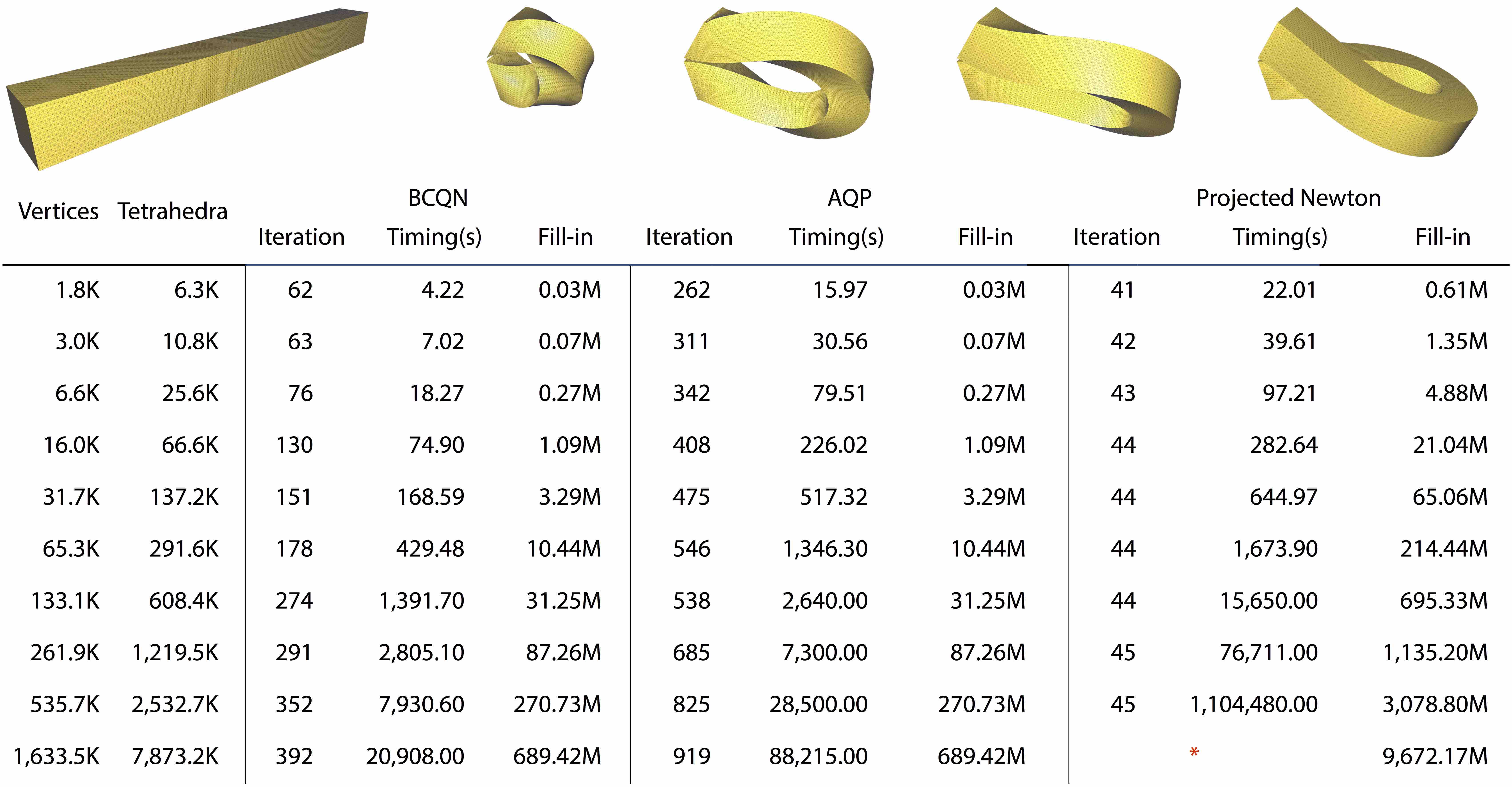
Figure 12: Three-Dimensional Deformation Scaling, Timing and Sparsity. Performance statistics and memory use for increasing mesh sizes up to 7.8M tetrahedra, comparing BCQN with AQP and PN. (CM does not extend to 3D.) We initialize a bar with a straight rest shape to start in a tightly twisted shape, constraining both ends to stay fixed and then optimize over increasing resolutions. For each method we report number of iterations to convergence (characteristic norm $<10^{-3}$), wall-clock time (seconds) to convergence, and the nonzero fill-in for the linear system solved by each method. We use * to indicate out of memory for the computation on our test system; see §8 for discussion.

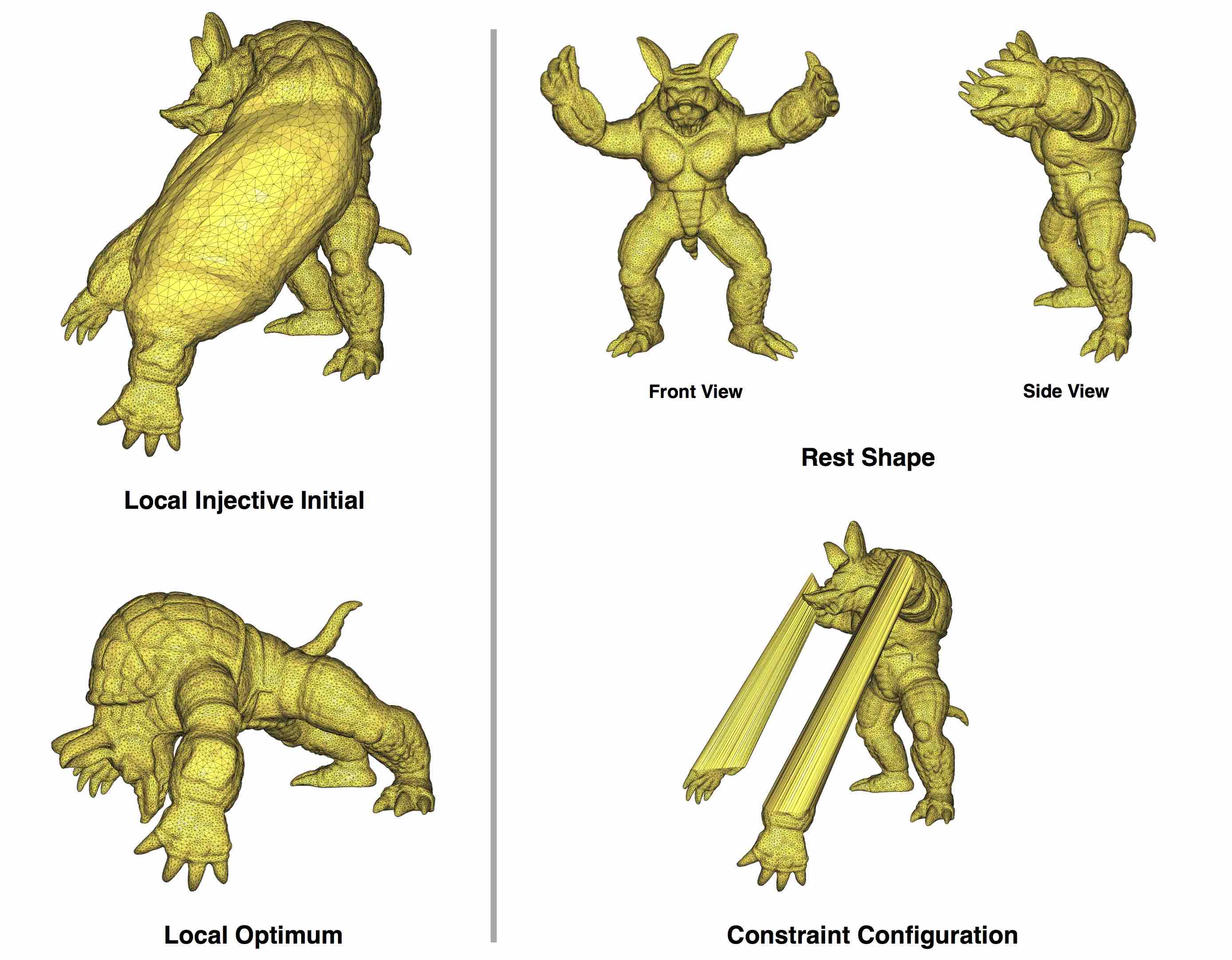
Figure 13: Armadillo Deformation Test. We compare three-dimensional deformation optimizations of a 1.5M element tetrahedral mesh of the T-pose armadillo with BCQN and PN. We constrain the armadillo’s feet to rest position, its hands to touch the ground and use the LBD method to create a locally injective initialization for the solvers. Here BCQN requires 393 iterations to converge while PN converges in just 9. However, as BCQN is much cheaper and more scalable per iterate it takes only 4,148 seconds, while PN spends 13,447 seconds.

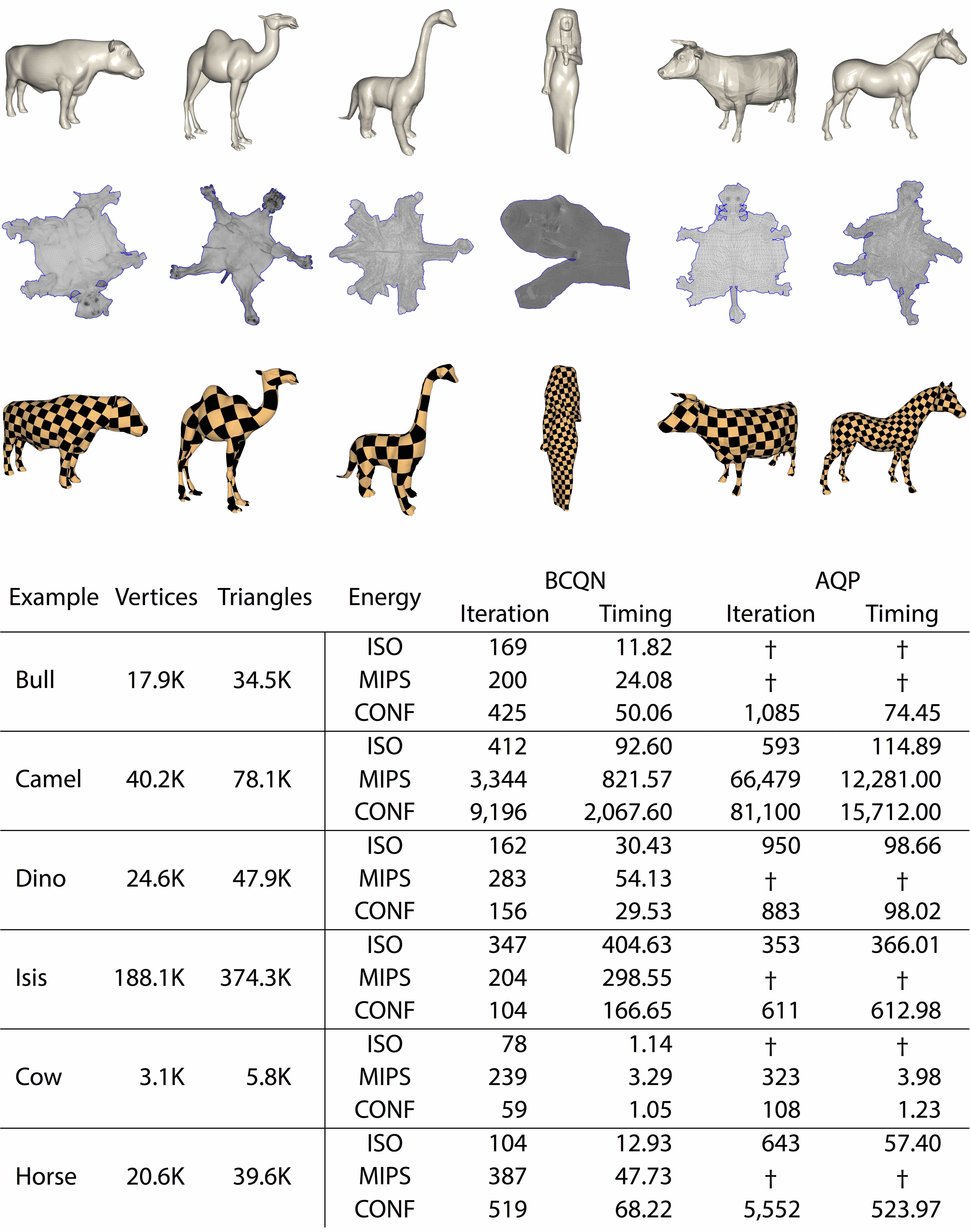
Figure 14: UV parameterization. Top row: 3D meshes for UV parametrization with ISO, MIPS, and CONF distortion energies. Middle two rows: converged maps and texturing from BCQN on ISO examples. Bottom: for each method / problem pair we report number of iterations to convergence (characteristic norm $<10^{-3}$) and wall-clock time (seconds) to convergence. We use ${\bf\dagger}$ to indicate when AQP does not converge; see §8.5.

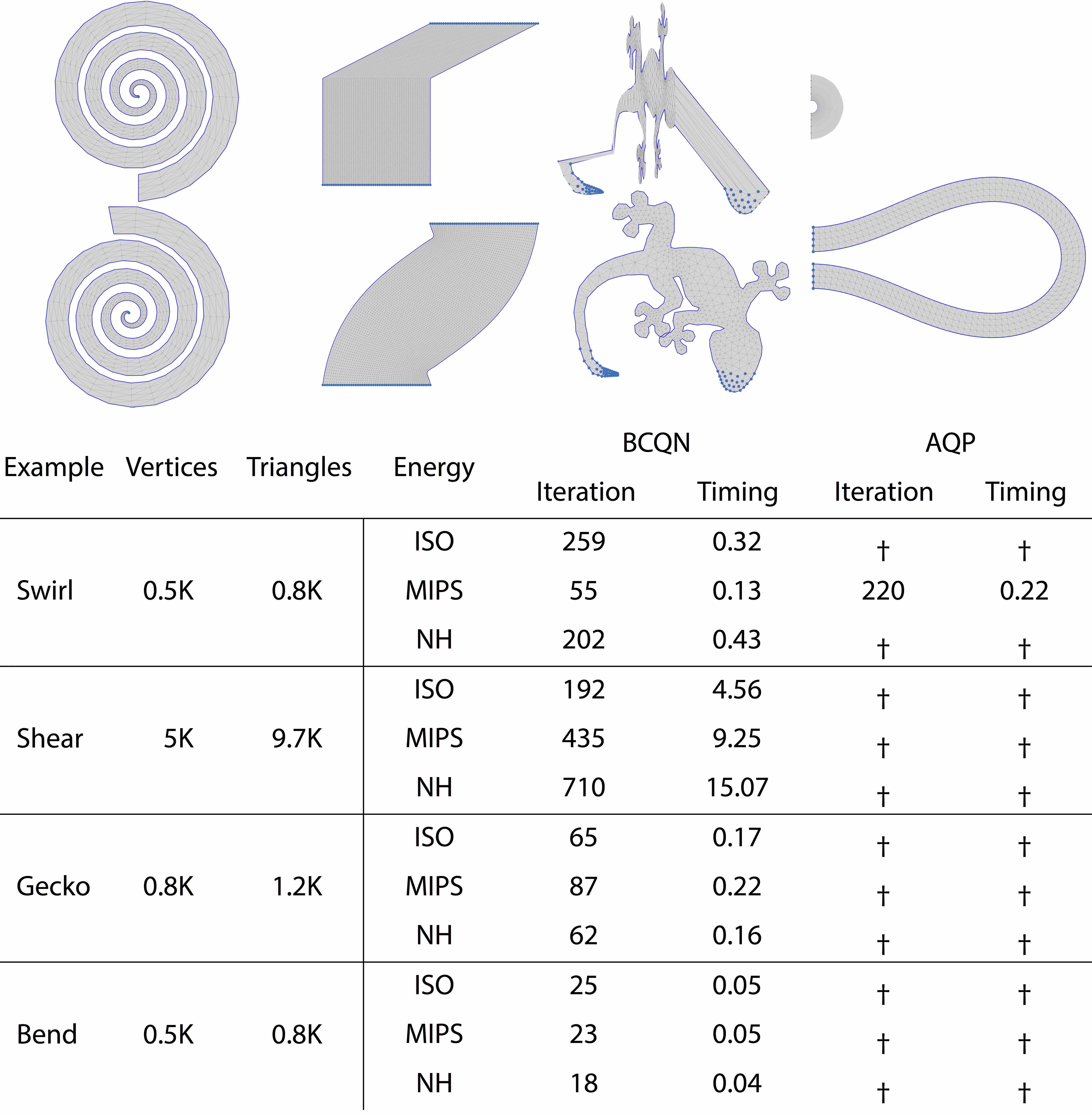
Figure 15: Two-Dimensional Deformation. Top: initial conditions and vertex constraints (blue points) for deformation problems minimizing ISO, MIPS, and NH deformation energies. Middle: converged solutions from BCQN on ISO examples. Bottom: for each method / problem pair we report number of iterations to convergence (characteristic norm $<10^{-3}$) and wall-clock time (seconds) to convergence. We use ${\bf\dagger}$ to indicate when AQP does not converge; see §8.5.

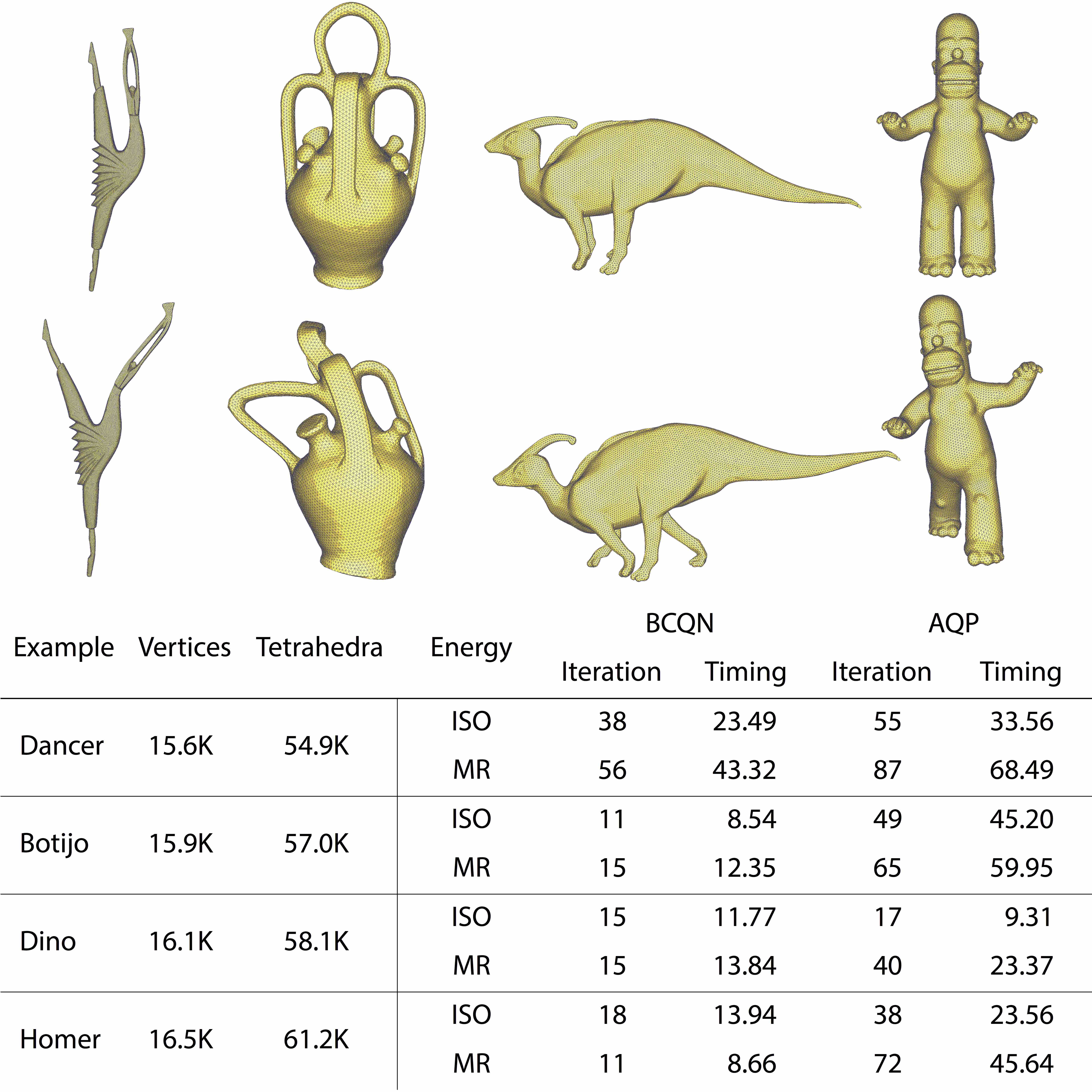
Figure 16: Three-Dimensional Deformation. Top: initial conditions for vertex-constrained deformation problems minimizing ISO and MR deformation energies. Middle: converged solutions satisfying constraints from BCQN on MR examples. Bottom: for each method / problem pair we report number of iterations to convergence (characteristic norm $<10^{-3}$) and wall-clock time (seconds) to convergence.

8.5 First-order methods

Among existing first-order methods for geometry optimization AQP has so far shown best efficiency [Kovalsky et al. 2016] with improved convergence over SGD as well as standard L-BFGS. Likewise, as we see in Figures 11, 12, and 13, when we scale to increasingly larger problems AQP will dominate over Newton-type methods and so potentially offers the promise of reliability across applications. Finally although small BQCN performs a small fixed amount of extra work per-iteration in the line-search filter and quasi-Newton update. Thus in Figures 11, 12, 14 and 16. we compare AQP and BCQN over a range of practical geometry optimization applications: respectively UV-parameterization, 2D deformation, and 3D deformation with nonconvex energies from geometry processing and physics. Throughout we note three key features distinguishing BCQN:

Reliability and robustness. AQP will fail to converge in some cases, see e.g. Figure 3, while BCQN reliably converges. In our testing AQP fails to converge in over 40% of our tests with nonconvex energies; see e.g. Figures 14 and 15. This behavior is duplicated in our test-harness code and AQP’s reference implementation.

Convergence speed. When AQP is able to converge, BCQN consistently provides faster convergence rates for nonconvex energies. In our experiments convergence rates range up to well over 10X with respect to AQP.

Performance. BCQN is efficient. When AQP is able to converge, BCQN remains fast with up to a well over 7X speedup over AQP on nonconvex energies.

8.6 Across the Board Comparisons

Here we compare the performance and memory usage of BCQN with best-in-class geometry optimization methods across the board: AQP, PN and CM for both 2D parameterization and 3D deformation tasks. Results are summarized in Figures 11, 12 and 13. Note that CM does not extend to 3D.

In Figures 11 and 12 we examine the scaling of AQP, PN, CM and BCQN to larger meshes and thus to larger problem sizes in both 2D parametrization (up to 23.9M triangles) and 3D deformation (up to 7.8M tetrahedra). As noted above: from the outset, BCQN requires more iterations than CM and PN; however, BCQN’s overall low cost per iteration makes it faster in performance across problem sizes when compared to both CM and PN. We then note that AQP, on the other hand, has slower convergence and so, at smaller sizes it often does not compete with CM and PN. However, once we reach larger mesh problems, e.g. $\sim\geq$ 6M triangles in Figure 11, the cost of factorization and backsolve of the denser linear systems of CM and PN becomes significant so that even AQP’s slower convergence results in improvement. This is the intended domain for which first-order methods are designed but here too, as we see in Figure 11, BCQN continues to outperform both AQP as well as CM and PN across all scales. Please see our supplemental video for visual comparisons of the relative progress of PN, CM, AQP and BCQN.

9 Conclusion

In this work we have taken new steps to both advance the state of the art for optimizing challenging nonconvex deformation energies and to better evaluate new and improved methods as they are subsequently developed. Looking forward these minimization tasks are likely to remain fundamental bottlenecks in practical codes and so advancement here is critical. Our three primary contributions together form the BCQN algorithm which pushes current limits in deformation optimization forward in terms of speed, reliability, and automatibility. At the same time looking ahead we also expect that each contribution individually should lead to even more improvements in the near future.

9.1 Limitations and Future Work

While our focus is on recent challenging nonconvex energies not addressed by the popular local-global framework, similar to AQP we have observed significant speedup for convex energies as well. Currently in comparing AQP and BCQN on the same set of 2D and 3D tasks with the convex ARAP energy we observe a generally modest improvement in convergence, up to a little over $4\times$, which is generally balanced by the small additional overhead of BCQN iterations. Note for energies like ARAP there is no barrier, hence no need for our line search filtering, but other opportunities for improvement may be abailable in future research.

While our current blending model works well in our extensive testing, it is empirically constructed; it is in no sense proven optimal. We believe that further analysis, better understanding and additional improvements in quasi-Newton blending are all exciting and promising avenues of future investigation.

Finally, we note that while we have focused here on optimizing deformation energies defined on meshes, there is a wide range of critical optimization problems that take similar general structure: minimizing separable nonlinear energies on graphs. Further extensions are thus exciting directions of ongoing investigation.

Appendix A Equivalence

Theorem. For our energy densities $W(\sigma)={f(\sigma)}/{g(\sigma)}$ with $f(\sigma)>0$ and $g(\sigma)\rightarrow 0$ as $\sigma\rightarrow 0$, $x^{*}$ is a stationary point of $\{E(x):a(x)\geq 0\}$ iff it is a locally injective stationary point of the unconstrained energy $E(x)$.

Proof.

The $1/g(\sigma)$ term drives element energies $W\big{(}F_{t}(x)\big{)}\rightarrow\infty$ as $a_{t}(x)\rightarrow 0$. Stationary points $x_{u}^{*}$ of unconstrained $E$ are given by $\nabla E(x_{u}^{*})=0$ and must satisfy $|a(x_{u}^{*})|>0$. The addition of local injectivity then requires $a(x_{u}^{*})>0$. Stationary points $x_{c}^{*}$ of $\{E(x)\>:\>a(x)\geq 0\}$ are given by the Karush-Kuhn-Tucker (KKT) conditions

$$\nabla E(x_{c}^{*})-\nabla a(x_{c}^{*})\lambda=0\>\>\text{and}\>\>0\leq\lambda\perp a(x_{c}^{*})\geq 0.$$ (28)

(Here $\lambda=(\lambda_{1},..,\lambda_{m})^{T}\in R^{m}$ is a Lagrange multiplier and $\mbox{{{$\mathsf{x}$}}}\perp\mbox{{{$\mathsf{y}$}}}$ is the complementarity condition $y_{t}z_{t}=0,\ \forall t$.) All $x_{u}^{*}$ satisfy (28) with $\lambda>0$. For $x_{c}^{*}$ satisfying (28) any $\lambda_{t}=0\implies a_{t}(x_{c}^{*})=0\implies W\big{(}F_{t}(x_{c}^{*})\big{)}=\infty$. Thus we must have $\lambda>0\implies a(x_{c}^{*})>0$ so that $x_{c}^{*}$ are locally injective stationary points of the unconstrained energy $E(x)$. ∎

References

- [\citenameAigerman et al. 2015] Aigerman, N., Poranne, R., and Lipman, Y. 2015. Seamless surface mappings. ACM Transactions on Graphics (TOG) 34, 4, 72.
- [\citenameBen-chen et al. 2008] Ben-chen, M., Gotsman, C., and Bunin, G. 2008. Conformal flattening by curvature prescription and metric scaling. COMPUTER GRAPHICS FORUM 27.
- [\citenameBertsekas 2016] Bertsekas, D. P. 2016. Nonlinear Programming. Athena Scientific.
- [\citenameBonet and Burton 1998] Bonet, J., and Burton, A. 1998. A simple orthotropic, transversely isotropic hyperelastic constitutive equation for large strain computations. Computer methods in applied mechanics and engineering 162, 1, 151–164.
- [\citenameBotsch et al. 2006] Botsch, M., Pauly, M., Gross, M. H., and Kobbelt, L. 2006. Primo: coupled prisms for intuitive surface modeling. In Symposium on Geometry Processing, no. EPFL-CONF-149310, 11–20.
- [\citenameBouaziz et al. 2012] Bouaziz, S., Deuss, M., Schwartzburg, Y., Weise, T., and Pauly, M. 2012. Shape-up: Shaping discrete geometry with projections. In Computer Graphics Forum, vol. 31, Wiley Online Library, 1657–1667.
- [\citenameBouaziz et al. 2014] Bouaziz, S., Martin, S., Liu, T., Kavan, L., and Pauly, M. 2014. Projective dynamics: fusing constraint projections for fast simulation. ACM Transactions on Graphics (TOG) 33, 4, 154.
- [\citenameBower 2009] Bower, A. F. 2009. Applied mechanics of solids. CRC press.
- [\citenameByrd et al. 1992] Byrd, R. H., Liu, D. C., and Nocedal, J. 1992. On the behavior of broyden’s class of quasi-newton methods. SIAM Journal on Optimization 2, 4, 533–557.
- [\citenameByrd et al. 1994] Byrd, R. H., Nocedal, J., and Schnabel, R. B. 1994. Representations of quasi-newton matrices and their use in limited memory methods. Mathematical Programming 63, 1-3, 129–156.
- [\citenameChao et al. 2010] Chao, I., Pinkall, U., Sanan, P., and Schröder, P. 2010. A simple geometric model for elastic deformations. ACM Transactions on Graphics (TOG) 29, 4, 38.
- [\citenameChen et al. 2008] Chen, Y., Davis, T. A., Hager, W. W., and Rajamanickam, S. 2008. Algorithm 887: Cholmod, supernodal sparse cholesky factorization and update/downdate. ACM Transactions on Mathematical Software (TOMS) 35, 3.
- [\citenameChen et al. 2013] Chen, R., Weber, O., Keren, D., and Ben-Chen, M. 2013. Planar shape interpolation with bounded distortion. ACM Transactions on Graphics (TOG) 32, 4, 108:1–108:12.
- [\citenameClaici et al. 2017] Claici, S., Bessmeltsev, M., Schaefer, S., and Solomon, J. 2017. Isometry-aware preconditioning for mesh parameterization. In Proceedings of the Symposium on Geometry Processing.
- [\citenameCottle et al. 2009] Cottle, R. W., Pang, J.-S., and Stone, R. E. 2009. The Linear Complementarity Problem. Society for Industrial & Applied Mathematics (SIAM).
- [\citenameDegener et al. 2003] Degener, P., Meseth, J., and Klein, R. 2003. An adaptable surface parameterization method. IMR 3, 201–213.
- [\citenameDesbrun et al. 2002] Desbrun, M., Meyer, M., and Alliez, P. 2002. Intrinsic parameterizations of surface meshes. In Computer Graphics Forum, vol. 21, Wiley Online Library, 209–218.
- [\citenameFischer 1992] Fischer, A. 1992. A special newton-type optimization method. 269–284.
- [\citenameFloater and Hormann 2005] Floater, M. S., and Hormann, K. 2005. Surface parameterization: a tutorial and survey. In Advances in multiresolution for geometric modelling. Springer, 157–186.
- [\citenameFu and Liu 2016] Fu, X.-M., and Liu, Y. 2016. Computing inversion-free mappings by simplex assembly. ACM Transactions on Graphics (TOG) 35, 6, 216.
- [\citenameFu et al. 2015] Fu, X.-M., Liu, Y., and Guo, B. 2015. Computing locally injective mappings by advanced mips. ACM Transactions on Graphics (TOG) 34, 4, 71.
- [\citenameGast et al. 2015] Gast, T. F., Schroeder, C., Stomakhin, A., Jiang, C., and Teran, J. M. 2015. Optimization integrator for large time steps. IEEE transactions on visualization and computer graphics 21, 10, 1103–1115.
- [\citenameHager 1984] Hager, W. W. 1984. Condition estimates. SIAM Journal on Scientific and Statistical Computing 5, 2.
- [\citenameHairer et al. 2006] Hairer, E., Lubich, C., and Wanner, G. 2006. Geometric Numerical Integration. Springer.
- [\citenameHecht et al. 2012] Hecht, F., Lee, Y. J., Shewchuk, J. R., and O’Brien, J. F. 2012. Updated sparse cholesky factors for corotational elastodynamics. ACM Transactions on Graphics (TOG) 31, 5, 123.
- [\citenameHormann and Greiner 2000] Hormann, K., and Greiner, G. 2000. Mips: An efficient global parametrization method. Tech. rep., DTIC Document.
- [\citenameHuang et al. 2006] Huang, J., Shi, X., Liu, X., Zhou, K., Wei, L.-Y., Teng, S.-H., Bao, H., Guo, B., and Shum, H.-Y. 2006. Subspace gradient domain mesh deformation. In ACM Transactions on Graphics (TOG), vol. 25, ACM, 1126–1134.
- [\citenameJiang et al. 2004] Jiang, L., Byrd, R. H., Eskow, E., and Schnabel, R. B. 2004. A preconditioned l-bfgs algorithm with application to molecular energy minimization. Tech. rep., DTIC Document.
- [\citenameJiang et al. 2017] Jiang, Z., Schaefer, S., and Panozzo, D. 2017. Simplicial complex augmentation framework for bijective maps. ACM Transactions on Graphics (TOG) 36, 6, 186:1–186:9.
- [\citenameKarush 1939] Karush, W. 1939. Minima of functions of several variables with inequalities as side constraints.
- [\citenameKovalsky et al. 2014] Kovalsky, S. Z., Aigerman, N., Basri, R., and Lipman, Y. 2014. Controlling singular values with semidefinite programming. ACM Trans. Graph. 33, 4, 68–1.
- [\citenameKovalsky et al. 2015] Kovalsky, S. Z., Aigerman, N., Basri, R., and Lipman, Y. 2015. Large-scale bounded distortion mappings. ACM Trans. Graph 34, 6, 191.
- [\citenameKovalsky et al. 2016] Kovalsky, S. Z., Galun, M., and Lipman, Y. 2016. Accelerated quadratic proxy for geometric optimization. ACM Transactions on Graphics (proceedings of ACM SIGGRAPH) 35, 4.
- [\citenameKuhn and Tucker 1951] Kuhn, H. W., and Tucker, A. W. 1951. Nonlinear programming. Proceedings of the Second Berkeley Symposium on Mathematical Statistics and Probability, 481—–492.
- [\citenameLevi and Weber 2016] Levi, Z., and Weber, O. 2016. On the convexity and feasibility of the bounded distortion harmonic mapping problem. ACM Transactions on Graphics (TOG) 35, 4, 106.
- [\citenameLevi and Zorin 2014] Levi, Z., and Zorin, D. 2014. Strict minimizers for geometric optimization. ACM Transactions on Graphics (TOG) 33, 6, 185.
- [\citenameLévy et al. 2002] Lévy, B., Petitjean, S., Ray, N., and Maillot, J. 2002. Least squares conformal maps for automatic texture atlas generation. In ACM Transactions on Graphics (TOG), vol. 21, ACM, 362–371.
- [\citenameLipman 2012] Lipman, Y. 2012. Bounded distortion mapping spaces for triangular meshes. ACM Transactions on Graphics (TOG) 31, 4, 108.
- [\citenameLipton et al. 1979] Lipton, R., Rose, D., and Targan, R. 1979. Generalized nested dissection. SIAM J. Numer. Anal. 16, 2, 346–358.
- [\citenameLiu et al. 2008] Liu, L., Zhang, L., Xu, Y., Gotsman, C., and Gortler, S. J. 2008. A local/global approach to mesh parameterization. In Computer Graphics Forum, vol. 27, Wiley Online Library, 1495–1504.
- [\citenameLiu et al. 2013] Liu, T., Bargteil, A. W., O’Brien, J. F., and Kavan, L. 2013. Fast simulation of mass-spring systems. ACM Transactions on Graphics (TOG) 32, 6, 214.
- [\citenameLiu et al. 2017] Liu, T., Bouaziz, S., and Kavan, L. 2017. Quasi-newton methods for real-time simulation of hyperelastic materials. ACM Transactions on Graphics (TOG) 36, 3, 23.
- [\citenameMartin et al. 2013] Martin, T., Joshi, P., Bergou, M., and Carr, N. 2013. Efficient non-linear optimization via multi-scale gradient filtering. In Computer Graphics Forum, vol. 32, Wiley Online Library, 89–100.
- [\citenameMooney 1940] Mooney, M. 1940. A theory of large elastic deformation. Journal of Applied Physics 11, 9, 582–592.
- [\citenameMullen et al. 2008] Mullen, P., Tong, Y., Alliez, P., and Desbrun, M. 2008. Spectral conformal parameterization. In Proceedings of the Symposium on Geometry Processing, Eurographics Association, SGP ’08, 1487–1494.
- [\citenameNarain et al. 2016] Narain, R., Overby, M., and Brown, G. E. 2016. Admm projective dynamics: Fast simulation of general constitutive models. In Proceedings of the ACM SIGGRAPH/Eurographics Symposium on Computer Animation, Eurographics Association, 21–28.
- [\citenameNesterov 1983] Nesterov, Y. 1983. A method of solving a convex programming problem with convergence rate O(1/sqr(k)). Soviet Mathematics Doklady 27, 372–376.
- [\citenameNeuberger 1985] Neuberger, J. 1985. Steepest descent and differential equations. Journal of the Mathematical Society of Japan 37, 2, 187–195.
- [\citenameNocedal and Wright 2006] Nocedal, J., and Wright, S. 2006. Numerical Optimization. Springer Series in Operations Research and Financial Engineering. Springer New York.
- [\citenameNocedal 1980] Nocedal, J. 1980. Updating quasi-newton matrices with limited storage. Mathematics of computation 35, 151, 773–782.
- [\citenameOgden 1972] Ogden, R. 1972. Large deformation isotropic elasticity – on the correlation of theory and experiment for incompressible rubberlike solids. In Proceedings of the Royal Society of London. Series A, Mathematical and Physical Sciences, 565–584.
- [\citenameParikh and Boyd 2014] Parikh, N., and Boyd, S. 2014. Proximal algorithms. Found. Trends Optim. 1, 3, 127–239.
- [\citenamePetra et al. 2014a] Petra, C. G., Schenk, O., and Anitescu, M. 2014. Real-time stochastic optimization of complex energy systems on high-performance computers. IEEE Computing in Science & Engineering 16, 5.
- [\citenamePetra et al. 2014b] Petra, C. G., Schenk, O., Lubin, M., and Gärtner, K. 2014. An augmented incomplete factorization approach for computing the schur complement in stochastic optimization. SIAM Journal on Scientific Computing 36, 2.
- [\citenamePoranne and Lipman 2014] Poranne, R., and Lipman, Y. 2014. Provably good planar mappings. ACM Transactions on Graphics (TOG) 33, 4, 76.
- [\citenameRabinovich et al. 2016] Rabinovich, M., Poranne, R., Panozzo, D., and Sorkine-Hornung, O. 2016. Scalable locally injective mappings.
- [\citenameRivlin 1948] Rivlin, R. S. 1948. Some applications of elasticity theory to rubber engineering. In Proc. Rubber Technology Conference, 1–8.
- [\citenameSchenk et al. 2001] Schenk, O., Gärtner, K., Fichtner, W., and Stricker, A. 2001. Pardiso: A high-performance serial and parallel sparse linear solver in semiconductor device simulation. Future Gener. Comput. Syst. 18, 1, 69–78.
- [\citenameSchüller et al. 2013] Schüller, C., Kavan, L., Panozzo, D., and Sorkine-Hornung, O. 2013. Locally injective mappings. In Computer Graphics Forum, vol. 32, Wiley Online Library, 125–135.
- [\citenameSheffer et al. 2006] Sheffer, A., Praun, E., and Rose, K. 2006. Mesh parameterization methods and their applications. Foundations and Trends® in Computer Graphics and Vision 2, 2, 105–171.
- [\citenameShtengel et al. 2017] Shtengel, A., Poranne, R., Sorkine-Hornung, O., Kovalsky, S. Z., and Lipman, Y. 2017. Geometric optimization via composite majorization. ACM Transactions on Graphics (TOG) 36, 4, 11.
- [\citenameSmith and Schaefer 2015] Smith, J., and Schaefer, S. 2015. Bijective parameterization with free boundaries. ACM Transactions on Graphics (TOG) 34, 4, 70.
- [\citenameSmith et al. 2012] Smith, B., Kaufman, D. M., Vouga, E., Tamstorf, R., and Grinspun, E. 2012. Reflections on simultaneous impact. ACM Transactions on Graphics (Proceedings of SIGGRAPH 2012) 31, 4, 106:1–106:12.
- [\citenameSorkine and Alexa 2007] Sorkine, O., and Alexa, M. 2007. As-rigid-as-possible surface modeling. In Symposium on Geometry processing, vol. 4.
- [\citenameStomakhin et al. 2012] Stomakhin, A., Howes, R., Schroeder, C., and Teran, J. M. 2012. Energetically consistent invertible elasticity. In Proceedings of the ACM SIGGRAPH/Eurographics Symposium on Computer Animation, Eurographics Association, 25–32.
- [\citenameTeran et al. 2005] Teran, J., Sifakis, E., Irving, G., and Fedkiw, R. 2005. Robust quasistatic finite elements and flesh simulation. In Proceedings of the 2005 ACM SIGGRAPH/Eurographics symposium on Computer animation, ACM, 181–190.
- [\citenameWang and Yang 2016] Wang, H., and Yang, Y. 2016. Descent methods for elastic body simulation on the gpu. ACM Transactions on Graphics (TOG) 35, 6, 212.
- [\citenameWang 2015] Wang, H. 2015. A chebyshev semi-iterative approach for accelerating projective and position-based dynamics. ACM Transactions on Graphics (TOG) 34, 6, 246.
- [\citenameWeber et al. 2012] Weber, O., Myles, A., and Zorin, D. 2012. Computing extremal quasiconformal maps. In Computer Graphics Forum, vol. 31, Wiley Online Library, 1679–1689.
- [\citenameXu et al. 2015] Xu, H., Sin, F., Zhu, Y., and Barbič, J. 2015. Nonlinear material design using principal stretches. ACM Transactions on Graphics (TOG) 34, 4, 75.