Parameter Estimation in Computational Biology by Approximate Bayesian Computation coupled with Sensitivity Analysis

Abstract

Motivation: We address the problem of parameter estimation in models of systems biology from noisy observations. The models we consider are characterized by simultaneous deterministic nonlinear differential equations whose parameters are either taken from in vitro experiments, or are hand-tuned during the model development process to reproduces observations from the system. We consider the family of algorithms coming under the Bayesian formulation of Approximate Bayesian Computation (ABC), and show that sensitivity analysis could be deployed to quantify the relative roles of different parameters in the system. Parameters to which a system is relatively less sensitive (known as sloppy parameters) need not be estimated to high precision, while the values of parameters that are more critical (stiff parameters) need to be determined with care. A tradeoff between computational complexity and the accuracy with which the posterior distribution may be probed is an important characteristic of this class of algorithms.
Results: With sensitivity analysis identifying the relative roles of different parameters, we show that a judicious allocation of computational budget can be made, achieving efficient parameter estimation. We demonstrate a three stage strategy, in which after identifying different parameters as sloppy and stiff, a coarse, computationally inexpensive step could be used to set the sloppy parameters. This is followed by an optimization stage with more stringent sample acceptance criteria to estimate stiff parameters. We also apply a recently developed adaptive algorithm for gradual cooling of the acceptance threshold within the ABC framework. We demonstrate the effectiveness of the proposed method on three models of oscillatory systems and one of transient response of an organism to heat shock, taken from the systems biology literature.
Contact:M.Niranjan@Southampton.ac.uk

1 Introduction

Computational modeling of biological systems is about describing quantitative relationships of biochemical reactions by systems of differential equations (Kitano, 2002). Knowledge of biological processes captured in such equations, when solutions to them match measurements made from the system of interest, help confirm our understanding of systems level function. Examples of such models include cell cycle progression (Chen et al., 2000), integrate and fire generation of heart pacemaker pulses (Zhang et al., 2000) and cellular behavior in synchrony with the circadian cycle (Leloup and Goldbeter, 2003). A particular appeal of modeling is that models can be interrogated with what if type questions to improve our understanding of the system, or be used to make quantitative predictions in domains in which measurements are unavailable.

A central issue in developing computational models of biological systems is setting parameters such as rate constants of biochemical reactions, synthesis and decay rates of macromolecules, delays incurred in transcription of genes and translation of proteins, and sharpness of nonlinear effects (Hill coefficient) are examples of such parameters. Parameter values are usually determined by conducting in vitro experiments (e.g. (Niedenthal et al., 1996; Wadsworth et al., 2001; Tseng et al., 2002; Wiedenmann et al., 2004)). When parameter values are not available from experimental measurements, modelers often resort to hand-tuning during the model development process and publish the range of values of a parameter required to achieve a match between model output and observed data. In dynamical systems characterized by variations over time, concentrations of different molecular species (proteins, metabolites etc.) may also be of interest. In this setting, we encounter two difficulties. First, parameters measured by in vitro experiments may not be good reflections of the in vivo reality. And, second, some parameters in a system may not be amenable to experimental measurements. These limitations motivate the need to infer parameters in a computational model based on input-output observations and recent literature on computational and systems biology has seen intense activity along these lines (Barenco et al., 2006; Vyshemirsky and Girolami, 2008; Jayawardhana et al., 2008; Henderson et al., 2010; Liu and Niranjan, 2012).

One way of setting parameters systematically is based in techniques for search and optimization. For example, Mendes and Kell (1998) compared several optimization based algorithms for estimating parameters along biochemical pathways, concluding that no single approach significantly outperforms other available approaches. Similar work on a developmental gene regulation circuit is described in Fomekong-Nanfack et al. (2009), and on a spline approximation based method for learning the parameters of enzyme kinetic model in a cell cycle system is described in Zhan and Yeung (2011).

An alternate approach is the use of probabilistic Bayesian formulations to quantify uncertainties in the process of estimating parameters. Work described in Golightly and Wilkinson (2005); Dewar et al. (2010); Barenco et al. (2006); Vyshemirsky and Girolami (2008); Jayawardhana et al. (2008) fall into this category. With time varying or dynamical systems, some authors have pointed out advantages of sequential estimation models, formulating the problem as state and parameter estimation in a state-space modeling framework (Quach et al., 2007; Sun et al., 2008; Lillacci and Khammash, 2010). Kalman filtering and its variants, and nonparametric particle filtering have been applied, in this setting (Yang et al., 2007; Liu and Niranjan, 2012).

An approach that has attracted much interest recently is the method of Approximate Bayesian Computation (ABC) or likelihood-free inference. While this approach has its roots in population genetics (Tavaré et al., 1997), where the likelihood is usually too complicated to write down in a computable form, it is also seen as a viable tool in systems biology parameter estimation problems ((Toni et al., 2009; Secrier et al., 2009)). In brief, the ABC approach assumes it is easier to simulate data from a model of interest than it is to compute and work with its likelihood under some assumed noise model. Hence a structured search could be carried out, in which one repeatedly simulates with parameter values sampled from a prior distribution, computes the error between simulated and observed data and decides to retain or reject a sample based on this error exceeding a threshold. Samples thus retained define a posterior density in the space of parameters to be estimated.

Several enhancements to this basic scheme of Tavaré et al. (1997) have been developed. Beaumont et al. (2002) used a weighted linear regression adjustment to improve the efficiency of search (ABC-Regression) with interesting applications (Hamilton et al., 2005). In systems biology, Toni et al. (2009) proposed a Sequential Importance Sampling (SIS) based ABC approach to infer the parameters of Lotka-Volterra and repressilator models. This ABC-SIS method was also utilized by Secrier et al. (2009) to estimate the parameters of mitogen-activated protein kinase (MAPK) signaling pathway (Krauss, 2006).

In implementing ABC algorithms, an inherent compromise between computational efficiency and accuracy of inference has to be made. This compromise is in the form of the acceptance threshold ($\epsilon$), also referred to as tolerance. Setting $\epsilon$ to a high value results in a large number of acceptances but the resulting inference will be inaccurate. Researchers use arbitrary user-specified approaches (Sisson et al., 2007; Beaumont et al., 2009; Toni et al., 2009) to deal with this issue, i.e. start with a large $\epsilon$ and progressively reduce in value as the algorithm converges. In an elegant piece of work recently, Del Moral et al. (2012) showed how such an $\epsilon$ scheduling approach can be adaptively set. For the ABC class of algorithms this adaptive technique is indeed a major breakthrough.

Chiachio et al. (2014) demonstrate the effectiveness of this adaptive ABC method by estimating parameters of two stochastic benchmark models (the second order moving average process and the white noise corrupt linear oscillator). Hainy et al. (2016) also used this algorithm to learn parameters in the spatial extremes model from the data on maximum annual summer temperatures from 39 sites in the Midwest region of the USA. In epidemiology, Lintusaari et al. (2016) utilized such likelihood-free approach to identify of transmission dynamic models for infectious diseases.

An additional point to consider, which we pursue in this work, is that in models of Systems Biology not all parameters behave in the same way. Gutenkunst et al. (2007) observe that in a large number of models, systems level behavior is not sensitive to some parameters while being critically sensitive to others. These are referred to as ‘sloppy’ and ‘stiff’ parameters, respectively. Over a wide range of values with sloppy parameters, system output varies very slightly, while even small changes to the setting of stiff parameters cause large perturbations in outputs. The ABC framework, with its analysis by synthesis structure, is ideally suited to exploit this observation as we demonstrate in this work. Additionally, we comment on the inherent compromise between accuracy and computational efficiency in choosing the number of particles and parallel filters for the adaptive ABC-SMC algorithm.

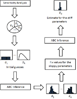
Figure 1: Computational steps in the proposed approach: Carrying the global sensitivity analysis technique (extended Fourier amplitude sensitivity test), we identify the sloppy and stiff parameters in system. Following this, starting from an initial guess of parameter values (most likely to be non-informative), we carry out estimation of parameters by Approximate Bayesian Computation (ABC) method associated with a coarse acceptance criterion. In the examples considered, we are using the advanced ABC algorithm for having the tolerance schedule adaptively. Details are described in Section 2.1. The sloppy parameters are then fixed to values determined by this coarse analysis. In the final stage, we estimate the stiff parameters of the system by running the ABC method to tighter error tolerance. This achieves a selective partitioning of the computational budget, and reliable estimates can be achieved within reasonable times.

2 Methods

The computational approach we propose, shown schematically in Fig. 1, is a combination of sensitivity analysis (Saltelli et al., 1999) and advanced ABC-SMC (Del Moral et al., 2012). We choose a particular method of sensitivity analysis (global sensitivity analysis, discussed later), to group the unknown parameters of a model into stiff and sloppy parameters. The sloppy parameters are estimated by a coarse search, which in ABC algorithms is achieved by using large values for acceptance thresholds. Once these are set, stiff parameters are estimated with adaptive evaluation of acceptance thresholds over a finer range.

We now summarize the methods of ABC-SMC with adaptive acceptance tolerance and the global sensitivity analysis techniques used in this work. We start with a succinct, tutorial type description of the ABC-SMC and Sensitivity Analysis frameworks, and present implemetation details to Supplementary Material.

2.1 Adaptive ABC-SMC

In parameter estimation problems, we seek a posterior distribution over parameters given observations, denoted $p(\boldsymbol{\theta}|\textbf{X})$. As noted in the Introduction, the basic idea in ABC algorithms is to sample the unknown from a prior distribution, $\theta^{\ast}\sim\pi(\theta)$, synthesize data from the model under study, $\textbf{X}^{\ast}\sim f(\textbf{x}_{0},\theta^{\ast})$, where $\textbf{x}_{0}$ is the initial condition and $f(\cdot,\cdot)$ is the model, and accept $\theta^{\ast}$ as a sample for the posterior if the synthesized data $\textbf{X}^{\ast}$ (referred to pseudo-observations in the following descriptions) is close enough in some sense to the observations X. In its earliest form (Tavaré et al., 1997), the generated particle $\theta^{\ast}$ was accepted only if $\textbf{X}^{\ast}$ was identical to the observations X. It became immediately evident that this is an inefficient procedure because thousands of trials needed to be performed before accepting one of the generated particles. A modification to the scheme, introduced by Pitt and Shephard (1999) was to define a tolerance $\epsilon$ and accept particles when the discrepancy between $\textbf{X}^{\ast}$ and X was smaller than this. In our discussion with Systems Biology models, we will focus on $f(\cdot,\cdot)$ being a set of ordinary differential equations which can be numerically integrated, and use Euclidean distance between the pseudo-observations and the model output as measure of discrepancy.

The Sequential Monte Carlo (SMC) method has recently been applied within the ABC setting (Sisson et al., 2007; Toni et al., 2009; Beaumont et al., 2009), in which, instead of synthesis from a single sample drawn from the prior being tested for acceptance of the sample, a population of samples is drawn, and progressively perturbed and synthesis from them tested for acceptance. At any stage, particles are drawn by sampling from the population of the previous stage in proportion to weights associated with them and perturbed via a transition kernel ${\theta}^{\ast\ast}\sim k({\theta}^{\ast})$. Pseudo-observations are then synthesized from the underlying model for the new population of samples: $\textbf{X}^{\ast}\sim f(\textbf{x}_{0},{\theta}^{\ast\ast})$. Particle ${\theta}^{\ast\ast}$ is accepted and weighted if the discrepancy between synthetic data $\textbf{X}^{\ast}$ and true dataset X is lower than the current tolerance $\epsilon_{t}$. To preserve diversity of particles, i.e. when {$\sum_{i=1}^{N_{\text{smc}}}{(w_{t}^{i})^{2}}\}^{-1}\leq\frac{N_{\text{smc}}}{2}$, resampling is also applied (Doucet et al., 2001). This population based approach is shown to result in more effective exploration of the space. Additionally, as mentioned before, the acceptance criterion is gradually reduced sequence of tolerance thresholds $\boldsymbol{\epsilon}=\{\epsilon_{1},\ldots,\epsilon_{T}\}$ at Sisson et al. (2007); Beaumont et al. (2009); Toni et al. (2009), in an arbitrary, user-defined way.

Del Moral et al. (2006) introduced a SMC sampler which constructs $M_{\text{smc}}$ (referred to integer factor) Markov kernels being operated in parallel. In the series of ABC developments, Del Moral et al. (2012) extended this concept to the ABC setting and formed an adaptive algorithm to determine the tolerance schedule $\boldsymbol{\epsilon}$. The weight calculation of this SMC sampler is given as

$${w}_{t}^{i} \propto{w}_{t-1}^{i}\frac{\sum_{m=1}^{M_{\text{smc}}}{\mathcal{I}_{\text{A}_{\epsilon_{t}}}(\textbf{S}_{m,t-1}^{\ast,i},\textbf{X})}}{\sum_{m=1}^{M_{\text{smc}}}{\mathcal{I}_{\text{A}_{\epsilon_{t-1}}}(\textbf{S}_{m,t-1}^{\ast,i},\textbf{X})}}$$ (1)

where $\textbf{S}^{\ast}\in\mathbb{R}^{M_{\text{smc}}\times N_{\text{smc}}\times D_{\text{s}}\times N_{\text{OT}}}$ are the pseudo-observations, and $\textbf{S}_{m,t-1}^{\ast,i}$ is the sub-block of pseudo-observations ($\textbf{S}_{m,t-1}^{\ast,i}$ is equivalent to aforementioned $\textbf{X}^{\ast}$) can be interpreted as the $m^{th}$ synthetic outputs generated by the $i^{th}$ parameter particle at $t$ iteration $\boldsymbol{\theta}_{t-1}^{i}$. $D_{\text{s}}$ and $N_{\text{OT}}$ are the dimension of states in system and the number of data points in output, respectively. $\mathcal{I}_{\epsilon_{t}}(\textbf{S}_{m,t-1}^{\ast,i},\textbf{X})$ is an indicator function that returns one if the discrepancy between pseudo-observation $\textbf{S}_{m,t-1}^{\ast i}$ and data X is less than the tolerance $\epsilon_{t}$, zero otherwise. A is the discrepancy, and which is measured by an Euclidean distance in this work.

By taking advantage of distribution of particles in the parallel filters, ABC-SMC is able to adaptively select the current tolerance level $\epsilon_{t}$. The idea behind this automatic scheme is to determine an appropriate reduction of the tolerance level based on the proportion of particles surviving under the current tolerance. If a large amount of particles remain ‘alive’, it implies the acceptance criterion is relatively loose and it is safe to make a jump for the next tolerance level. In contrast, if the ratio of ‘alive’ particles is low, this means that particles are less likely to describe the posterior and therefore, a tiny movement should be considered.

Given the proportion of ‘alive’ particles by

$$\text{PA}(\textbf{w}_{t},\epsilon_{t})=\frac{\sum_{i=1}^{N_{\text{smc}}}{\mathbb{I}_{(0,\infty)}({w}_{t}^{i})}}{N_{\text{smc}}}$$ (2)

the next tolerance level $\epsilon_{t+1}$ is chosen by making such proportion equals to a given percentage of the current tolerance $\text{PA}(\textbf{w}_{t},\epsilon_{t+1})=\alpha_{\text{smc}}\text{PA}(\textbf{w}_{t},\epsilon_{t})$, where $\alpha_{\text{smc}}$ is the tolerance reduction factor. The search of $\epsilon_{t+1}$ is achieved by fzero function in Matlab via setting the starting point to $\epsilon_{t}$.

To solve ODEs in use of running filters parallel, the initial conditions are set to $\widehat{\textbf{X}}_{0}\sim\mathcal{U}(\textbf{x}_{0},k\textbf{x}_{0})$, where $\widehat{\textbf{X}}_{0}\in\mathbb{R}^{M_{\text{smc}}\times\text{D}_{\text{s}}}$, $\textbf{x}_{0}$ is ‘true’ initial values for generating observations and $k$ is the scaling factor to control consistency/inconsistency of initial conditions across filters. Additionally, for moving particles to explore the parameter space, similarly to the previous work (Liu and Niranjan, 2012), we use the kernel smoothing with shrinkage as parameter evolution (Liu and West, 2001), instead of random walk kernel. The details and pseudo-code of ABC-SMC can be found in Section 2 of Supplementary materials accompanying the online version of this paper.

The Matlab code of proposed method is available at: https://github.com/brianliu2/ABCSMC-SA

2.2 Extended Fourier Amplitude Sensitivity Test

The extended Fourier amplitude sensitivity test (eFAST) (Saltelli et al., 1999) is one of the global sensitivity analysis techniques, which is derived by decomposing variance and claimed to be applicable for analyzing the nonlinear and non-monotonic systems. It has been successfully deployed to analyze the property of parameters in TCR-activated MAPK signalling pathway model (Zheng and Rundell, 2006) and thermodynamics gene expression model (Dresch et al., 2010). The algorithm initially partitions the total variance of the data, evaluating what fraction of the variance can be determined by variations in the parameter of interest. This quantity, known as the sensitivity index, defines the property of stiff or sloppy, is calculated as

$$\text{SI}=\frac{\text{Var}_{\boldsymbol{\theta}}[\text{E}(\textbf{X}^{\ast}|\boldsymbol{\theta})]}{\text{Var}(\textbf{X}^{\ast})}=\frac{V_{\theta}}{V}.$$ (3)

The variance is calculated with respect to sets of synthesis which are generated by solving the model associated with samples of parameters. In order to draw samples for parameters, Saltelli (2002) derived a heuristic sinusoidal function, given as

$$\boldsymbol{\theta} =G(\sin(\boldsymbol{\omega}\boldsymbol{s}+\boldsymbol{\varphi}))$$

$$=\frac{1}{2}+\frac{1}{\pi}\arcsin(\sin(\boldsymbol{\omega}\boldsymbol{s}+\boldsymbol{\varphi})),$$ (4)

where $\boldsymbol{\varphi}$ is the $D_{\text{p}}\times N_{\text{se}}$ matrix for providing random phase-shifting and which follows uniformly distributed $[0,2\pi]$. $N_{\text{se}}$ specifies the number of samples drawn from the function $G(\cdot)$. $D_{\text{p}}$ is the dimension of parameters in system. $\boldsymbol{s}$ in Eqn. (2.2) defines a $1\times N_{\text{se}}$ equally spaced vector where each interval is equally distributed from $-\pi$ to $\pi$. In this scheme, it is crucial to properly determine the frequency vector $\boldsymbol{\omega}:D_{\text{p}}\times 1$, in which the highest value referred to maximum frequency $\omega_{\text{max}}=(N_{\text{se}}-1)/2M_{\text{e}}$ is assigned to the parameter under study. $M_{\text{e}}$ is known as the interference factor and acts as the remover for numerical amplitude from superposing of waves. From the empirical investigation (Saltelli, 2002; Marino et al., 2008b), it is usually used as 4 or 6 (we use 4 in this work). Other frequencies in $\boldsymbol{\omega}$ are set in the range $[1,\ \omega_{-i,\text{max}}]$ with a regular increment $\frac{\omega_{-i,\text{max}}}{D_{\text{p}}}$, where $\omega_{-i,\text{max}}=\frac{\omega_{\text{max}}}{2M_{\text{e}}}$.

This strategy means that the sensitivity of underlying parameter is assessed by picking the samples with the highest frequency $\omega_{\text{max}}$, while the samples for the rest of the parameters are selected with the complementary frequencies $\boldsymbol{\omega}_{-i}$. This process is repeated until the samples of each parameter is drawn with highest frequency once. An illustrative example of this cycling process is shown in Fig. 2.

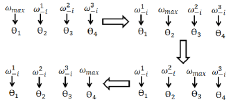
Figure 2: When we wise to evaluate the sensitivity of parameter $\theta_{1}$, its samples are drawn with the highest frequency $\omega_{\text{max}}$, while the samples for other parameters $\boldsymbol{\theta}_{-i}=\{\theta_{2},\ \theta_{3},\ \theta_{4}\}$ in the system are picked using the complementary frequencies $\boldsymbol{\omega}_{-i}=\{\omega^{1}_{-i},\ \omega^{2}_{-i},\ \omega^{3}_{-i}\}$. Through this process, all parameters in system should be assigned to the highest frequency once.

Consequently, the parameter can be seen as the most sensitive when which has the largest normalized variance, i.e. its variation causes the highest uncertainty. In addition, for any sample of parameter drawn from the unit hypercube $\boldsymbol{K}^{i}=(\boldsymbol{\theta}|0\leq\theta_{i}\leq 1;\ i=1,\ldots,D_{\text{p}})$, it has to be re-scaled to real-valued space as such the model evaluation can be carried out. Hence, a non-informative prior covered whole range of parameter value is required. In this work, we consider the suggestion from Marino et al. (2008a), where authors claimed that eFAST artificially yields small but non-zero sensitivity indexes for parameters, and thus a ‘dummy’ parameter which does not really exist in model and has no influence on behaving dynamics in any way, is introduced in eFAST to absorb such artifacts. The complete description of eFAST including the mathematical derivation and pseudo-code are presented in Section 3 of Supplementary materials.

3 Results and Discussion

We demonstrate the effectiveness of the proposed method using three models of sustained periodic oscillations and and one model of transient response to shock. These are models used by previous authors, including ourselves, enabling comparisons to be made. We give details of implementation in Section 6 of Supplementary materials. Crucial results from the heat shock and repressilator systems are discussed here and results from the remaining two systems are given in Supplementary materials.

The heat shock model We consider the case of estimating all six parameters of this model simultaneously. This is the most difficult case considered in our previous work (Liu and Niranjan, 2012), in which particle filters were able to correctly estimate four of the six unknown parameters, and failed in the remaining two ($k_{d}$ and $\alpha_{d}$). Fig. 3.A shows results of sensitivity analysis of one of the states $S_{t}$ (see equations of the system in Supplementary materials). Of these, parameters $\alpha_{d}$, $k_{d}$ and $\alpha_{0}$, to which $S_{t}$ is most sensitive to, are treated as stiff and the remainder as sloppy. Posterior distributions over estimates of the stiff parameters, using the proposed method, are shown in Fig. 3.C and the corresponding sloppy ones are given in Fig. S1(c). While the posterior means of $k_{d}$ and $\alpha_{d}$ are estimated to a high level of accuracy, $\alpha_{0}$ is not. This is explained by the sensitivity results in which we note that, though we took all these three to be stiff parameters, the state is not as sensitive to $\alpha_{0}$ as it is to $k_{d}$ and $\alpha_{d}$. Hence, relatively poor estimates of $\alpha_{0}$ will still lead to accurate reconstruction of the model outputs.

In Fig. 3.B, we show two responses synthesized from the posterior mean values of particle distributions from a classic particle filtering approach (as considered in our previous work, Liu and Niranjan (2012)) and the ABC-SMC method proposed here. We note that in this difficult problem of estimating all six parameters of the model, ABC-SMC is able to successfully find solutions of parameters from which the underlying state could be accurately generated for the state $S_{t}$ in the heat shock model. We observe the same to be true for the other two states, $D_{t}$ and $U_{f}$ as well (graphs shown in Fig. S1.(a) of Supplementary materials).

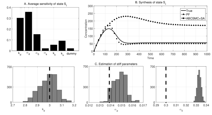
Figure 3: Sensitivity analysis, inference of parameters and system re-synthesis of heat shock model. A: Average sensitivity of parameters with respect to state $S_{t}$. B: Reproduction of state $S_{t}$ by using true values, estimates from ABC+SA (dotted line) and PF (dotted triangle) respectively. C:Histograms for the stiff parameters $k_{d}$, $\alpha_{d}$ and $\alpha_{0}$. The black lines indicate the true values of parameters proposed in the literature.

Repressilator system The deterministic repressilator system is constructed as a synthetic gene regulatory circuit which can sustain oscillations by the mutual repression of gene transcription (Elowitz and Leibler, 2000). This system consists of six differential equations, from three pairs of mRNA and protein, and has four parameters. This system was analysed by Toni et al. (2009) to demonstrate their ABC-SIS approach.

While we have set the posterior means of a coarse search to sloppy parameters ($\alpha$ and $\beta$), ABC-SMC is capable to find accurate solutions of stiff parameters, given allocated extra computational budget. Posterior distributions of a stiff ($\alpha_{0}$) and sloppy ($\alpha$) parameters from our proposed method and its predecessor ABC-SIS are shown in Fig.4.B-E. We note that, with an identical tight acceptance condition $\epsilon_{T}$, both methods are adequate in estimating stiff parameters to a relatively high level of accuracy. However, ABC-SIS shows a distinguishable advantage in identifying sloppy parameters, whereas our proposed method fails to achieve convergence to the correct estimate. Reconstruction of model behavior, using the posterior mean values from both methods, tells that the failure of finding solutions for sloppy parameters does not hugely hamper the effectiveness in characterizing dynamics. The complete results are shown as color figure in Fig. S2-S3 of Supplementary materials. In addition, we also tested how sensitivity analysis affects ABC-SMC by setting all possible combinations of stiffness/sloppiness to parameters, we found that at lease one stiff parameter is correctly chosen, ABC-SMC is able to find solutions. Results are given in Table S7.

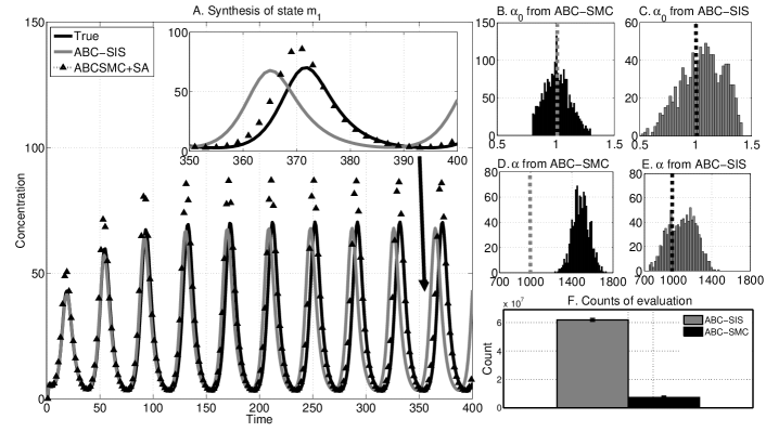
Figure 4: System synthesis, inference and computational performance: A: Synthesis of system behavior by using the true values from literature, inferred values from two methods. The proposed method (denoted by dotted triangle) captures the system behavior in terms of periodicity, but with larger amplitude. ABC-SIS successfully recovers the maximum, while a slight offset occurs in the last few time instants. The zoom-in version concentrates the last periodicity. The clear and color version of these graphs are given as Fig.S2. B-C: The estimates of stiff parameter $\alpha_{0}$ from ABC-SMC+SA and ABC-SIS. D-E: The estimates of sloppy parameter $\alpha$ from ABC-SMC+SA and ABC-SIS. In these graphs, the dash lines indicate the true values of corresponding parameters. F: Counts of model evaluation taken by ABC-SIS and the ABC-SMC+SA to achieve the final tolerance $\epsilon_{T}$.

In order to show how ABC-SIS is influenced by the suboptimal user-specific algorithmic setting, we compare the computational expense between ABC-SIS and our proposed method using identical initial and final tolerances. Since ABC-SMC on average requires 140 iterations to reach $\epsilon_{T}$, we therefore reduce the tolerance from $\epsilon_{0}$ down to $\epsilon_{T}$ using 140 steps at regular intervals. The algorithm efficiency is quantified by counting the number of model evaluations, at which most of computational budget is spent, to reach final tolerance $\epsilon_{T}$. Fig. 4.F clearly shows that the number of evaluations made by ABC-SIS is approximately seven times greater than ABC-SMC. This is because the suboptimal chosen transition kernel and tolerance schedule make ABC-SIS expend considerable computation on searching for acceptable particles.

Other systems We further consider delay-driven oscillatory system and cell cycle system, for which the complete descriptions and results are given in Section 4.3 and Section 4.4 of Supplementary materials.

In the delay-driven oscillatory example, for testing the general advantage of proposed method, we use the non-sophisticated ABC-MCMC (Marjoram et al., 2003) instead of ABC-SMC in this example. From the results given in Fig. S4, it is easy to observe that the original ABC-MCMC poorly performs with the coarse acceptance criterion, while it can produce the accurate inference by using a small tolerance $\epsilon$. When the similar precision of inferences is achieve, as expected, the proposed method greatly outperforms in efficiency (the comparison is shown in Fig. S4.F).

The cell cycle system, with 12 free parameters in the model, is a relatively high dimensional system. When particles are sampled in this space, we found that for a significant fraction of the samples, the ODE solver failed to terminate. With the proposed method, because sensitivity analysis identifies the sloppy parameters which have been set to the posterior means of a coarse search, the dimensionality is reduced and this issue gets circumvented.

However, since the state $RA$ in this cell cycle has no influential parameter in behaving dynamics (sensitivity analysis with respect to $RA$ is given in Fig. S8), therefore, a favorable computational budget allocation for state $RA$ can only be provided by associating the higher-order sensitivity index (influence on outputs caused by the interaction between parameters).

Effect of $M_{\text{smc}}$ and $N_{\text{smc}}$ In running ABC-SMC algorithms, we would ideally like to choose large values for $M_{\text{smc}}$ and $N_{\text{smc}}$ for achieving high accuracy of exploring the posterior density. Naturally, this will increase the computational complexity of the implementation. How does one trade-off spending a given computational budget across $M_{\text{smc}}$ (the number of parallel filters) and $N_{\text{smc}}$ (the number of particles per filter)? The choice is likely to be problem dependent, but an empirical exploration, using the repressillator system, over three sets of values for these $M_{\text{smc}}$ = 20 and $N_{\text{smc}}$ = 2, 000; $M_{\text{smc}}$ = 200 and $N_{\text{smc}}$ = 200; and $M_{\text{smc}}$ = 2, 000 and $N_{\text{smc}}$ = 20, keeping their product at 40, 000, is shown in Fig. 5. The corresponding accuracies of inference are given in Table 1.

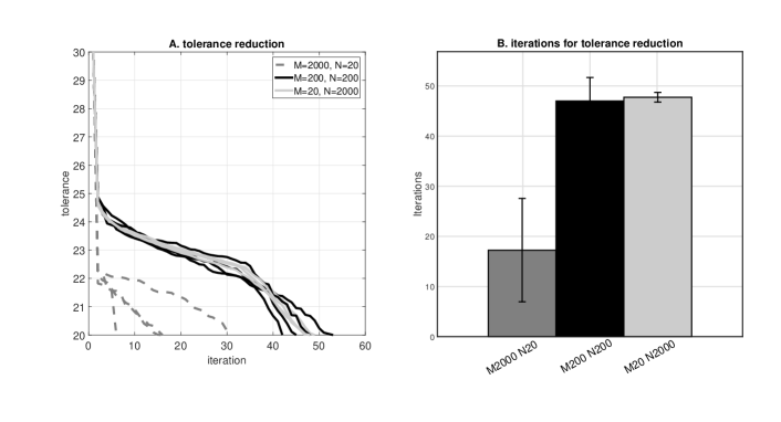
Figure 5: Effect of $M_{\text{smc}}$ versus $N_{\text{smc}}$ on approaching target tolerance $\epsilon_{T}$ . The total amount of particles remains the same, i.e. 40,000, and particles are distributed in different settings of $M_{\text{smc}}$ and $N_{\text{smc}}$. The above example, three combinatins are examined: $M_{\text{smc}}$ = 2, 000 and $N_{\text{smc}}$ = 20; $M_{\text{smc}}$ = 200 and $N_{\text{smc}}$ = 200; $M_{\text{smc}}$ = 20 and $N_{\text{smc}}$ = 2, 000. Each combination is carried out 4 times on the repressilator system. A: Trajectories of approaching target tolerance $\epsilon_{T}$ by different combinations. B: Average iterations carried out by different combinations. Overlapping graphs are presented more clearly as color figure in Fig. S12 of Supplementary materials.

Table 1: Comparison of NRMSE for different settings of $M_{\text{smc}}/N_{\text{smc}}$

		NRMSE
$M_{\text{smc}}$	$N_{\text{smc}}$	$\alpha_{0}$	$n$	$\beta$	$\alpha$
2000	20	6.41$\pm$2.71	1.92$\pm$0.20	1.01$\pm$0.20	1.04$\pm$0.34
200	200	6.17$\pm$0.72	1.21$\pm$0.04	1.21$\pm$0.10	1.11$\pm$0.10
20	2000	5.20$\pm$0.45	1.11$\pm$0.04	1.03$\pm$0.05	0.99$\pm$0.02

As seen in the graphs, smaller values of $M_{\text{smc}}$ are computationally less expensive. This is due to lower value of $M_{\text{smc}}$ causing a higher probability of particles being ‘killed’ and having a zero weight. As as consequence, decrements taken in $\boldsymbol{\epsilon}$ are smaller slowing convergence to its target $\epsilon_{\text{T}}$. For instance, considering the large $M_{\text{smc}}$ example, i.e. $M_{\text{smc}}$ = 2000, evaluating importance using Eqn.1, the zero weight barely appears. Intuitively, the greater non-zero proportion of the weight vector implies that most particles fulfill the current acceptance criterion, therefore, a large decrement should be taken for the next tolerance level. From the perspective of accuracy, when gaining a larger number of particles, the diversity of realizations increases and better performance in terms of precision is naturally expected. This conclusion is verified by the comparison of Normalized Root Mean Squared Error (NRMSE) which is a measurement to quantify the quality of prediction and its expression is given as:

$$\text{NRMSE}=\frac{\sqrt{\frac{\sum_{i=1}^{N}{\widehat{\theta}_{i}-\theta_{\text{true}}}}{N}}}{\max({\widehat{\boldsymbol{\theta}}})-\min({\widehat{\boldsymbol{\theta}}})}$$ (5)

From the results shown in Table 1, the higher $N_{\text{smc}}$ value generally delivers the better inference, where $N_{\text{smc}}$ = 2000 performs best among all considered settings.

Why use eFAST for sensitivity analysis? We have chosen eFAST, a global method, for sensitivity analysis in this work. The search carried out by this method, systematically exploring a wide range in the parameter space is computational expensive. An alternate method of quantifying parameter sensitivities, particularly in the context of particle filtering, adopted by Toni et al. (2009) is based on principal component analysis (PCA) of the particle distribution, and to use the principal directions as indicators of sloppy and stiff directions of parameter combinations. Parameters that are well aligned to the directions may show the declared stiff and sloppy. However, this simplistic approach is inadequate for our purpose for two reasons. Firstly, we wish to identify sloppy and stiff parameters of the models before running the particle filters, hence PCA on the distribution of a converged solution is not very useful. Secondly, and somewhat more importantly, PCA is a good representation of data that is multivariate Gaussian. If we expect the distribution of particles to be multivariate Gaussian, we would not be running particle filtering anyway, because Kalman filter type updates of posterior means and covariances are the known optimal solutions. In order to confirm this, we took the distributions of particles, after convergence, of all the four models considered and tested them for multivariate Gaussianity using Henze-Zirkler (multivariate normality) test (Henze and Zirkler, 1990). Such test is carried out upon measuring the non-negative functional distance between two distributions. If data of interest are distributed as multivariate normal, the test statistic is approximately log-normally distributed. The function hzTest from R package MVN (Korkmaz et al., 2014) is used in this work. From the test, we found three of them to be non-Gaussian. This confirms that the choice of global variance based sensitivity analysis is the correct one for our analysis.

4 Conclusion

In this work, we proposed an inference method for analyzing Systems Biology models that couples sensitivity analysis and approximate Bayesian computation. Our proposed method is particularly advantageous in difficult settings of estimating all (or most of) the parameters of a model from noisy observations, because it strikes a balance between accuracy and efficiency. The method exploits the fact that all parameters in model have different significance in characterizing model dynamics in terms of their sensitivities. By re-synthesis data from models with estimated parameters, we show that the values of parameters that are more critical (stiff parameters) need to be determined with care, while the sloppy parameters need not be estimated to high precision. To facilitate such inference, we have proposed a three stage strategy in which a selective computational budget allocation is implemented via sensitivity analysis, in which the sloppy group is estimated by a coarse search followed the re-estimation of stiff parameters to tighter error tolerances.

We have demonstrated the effectiveness of the proposed approach on three systems of oscillatory behavior and one of transient response. The results show that the introduction of favorable inference strategy allows to reduce the dimension of unknown parameters, and paves a potential way to tackle the complex problems. Additionally, the used ABC-SMC has attracted much interest due to its adaptivity in determining tolerance schedule $\boldsymbol{\epsilon}$ and the ‘no rejection’ of particles allows to boost the efficiency via parallel computing. In the simple problem, e.g. the delay-driven oscillatory system, with performing similarly in accuracy, the proposed inference method expends much less computational cost than the existed ABC methods.

References

- Barenco et al. (2006) M Barenco, D Tomescu, D Brewer, R Callard, J Stark, and M Hubank. Ranked prediction of p53 targets using hidden variable dynamic modeling. Genome Biology, 7(3):R25, 2006.
- Beaumont et al. (2009) M. Beaumont, C. P. Robert, J. M. Marin, and J. M. Cornuet. Adaptivity for ABC algorithms: the ABC-PMC scheme. Biometrika, 94(4):983–990, 2009.
- Beaumont et al. (2002) M. A. Beaumont, W. Zhang, and D. J. Balding. Approximate bayesian computation population genetics. Genetics, 162(4):2025–2035, 2002.
- Chen et al. (2000) K. C. Chen, A. Csikasz-Nagy, B. Gyorffy, J. Val, B. Novak, and J. J. Tyson. Kinetic analysis of a molecular model of the budding yeast cell cycle. Mol. Biol. Cell, 11(12):369–391, 2000.
- Chiachio et al. (2014) M. Chiachio, J. L. Beck, J. Chiachio, and G. Rus. Approximate Bayesian computation by subset simulation. SIAM Journal on Scientific Computing, 36(3):A1339–A1358, 2014.
- Del Moral et al. (2006) P. Del Moral, A. Doucet, and A. Jasra. Sequential Monte Carlo samplers. J. R. Stat. Soc. B, 68(3):411–436, 2006.
- Del Moral et al. (2012) P. Del Moral, Arnaud. Doucet, and A. Jasra. An adaptive sequential monte carlo method for approximate bayesian computation. Stat. Comput, 22(5):1009–1020, 2012.
- Dewar et al. (2010) M. A. Dewar, V. Kadirkamanathan, M. Opper, and G. Sanguinetti. Parameter estimation and inference for stochastic reaction-diffusion systems: application to morphogenesis in D. melanogaster. BMC Systems Biology, 4(1):21, 2010.
- Doucet et al. (2001) A. Doucet, J. F. G. de Freitas, and N. Gordon. Sequential Monte Carlo Methods in Practice. Springer, 2001. ISBN 978-0387951461.
- Dresch et al. (2010) J. M. Dresch, X. Liu, D. N. Arnosti, and A. Ay. Thermodynamic modeling of transcription: sensitivity analysis differentiates biological mechanism from mathematical model-induced effects. BMC systems biology, 4(1):142, 2010.
- Elowitz and Leibler (2000) M. B. Elowitz and S. Leibler. A synthetic oscillatory network of transcriptional regulators. Nature, 403(6767):335–338, 2000.
- Fomekong-Nanfack et al. (2009) Yves Fomekong-Nanfack, Marten Postma, and Jaap. A. Kaandorp. Inferring Drosophila gap gene regulatory network: a parameter sensitivity and perturbation analysis. BMC Systems Biology, 3(1):94, 2009. ISSN 1752-0509.
- Golightly and Wilkinson (2005) A. Golightly and D. J. Wilkinson. Bayesian inference for stochastic kinetic models using a diffusion approximation. Biometrics, 61(3):781–788, 2005.
- Gutenkunst et al. (2007) R. N. Gutenkunst, J. J. Waterfall, F. P. Casey, K. S. Brown, C. R. Myers, and J. P. Sethna. Universally sloppy parameter sensitivities in systems biology models. PLoS Comput. Biol., 3(10):e189, 2007.
- Hainy et al. (2016) M. Hainy, W. G. Müller, and H. Wagner. Likelihood-free simulation-based optimal design with an application to spatial extremes. Stochastic Environmental Research and Risk Assessment, 30(2):481–492, 2016.
- Hamilton et al. (2005) G. Hamilton, M. Stoneking, and L. Excoffier. Molecular analysis reveals tighter social regulation of immigration in patrilocal populations than in matrilocal population. Proc. Natl. Acad. Sci, 102(21):7476–7480, 2005.
- Henderson et al. (2010) D. A. Henderson, R. J. Boys, C. J. Proctor, and D. J. Wilkinson. Linking systems biology models to data: a stochastic kinetic model of p53 oscillations. In A. O’Hagan and M. West, editors, Handbook of applied Bayesian analysis, pages 155–187. Oxford University Press, 2010.
- Henze and Zirkler (1990) N. Henze and B. Zirkler. A class of invariant consistent tests for multivariate normality. Communications in Statistics-Theory and Methods, 19(10):3595–3617, 1990.
- Jayawardhana et al. (2008) B. Jayawardhana, D. B. Kell, and M. Rattray. Bayesian inference of the sites of perturbations in metabolic pathways via Markov Chain Monte Carlo. Bioinformatics, 24(9):1191–1197, 2008.
- Kitano (2002) H. Kitano. Systems biology: A brief overview. Science, 295(5560):1662–1664, 2002.
- Korkmaz et al. (2014) S. Korkmaz, D. Goksuluk, and G. Zararsiz. MVN: an R package for assessing multivariate normality. The R Journal, 6(2):151–162, 2014.
- Krauss (2006) G. Krauss. Biochemistry of signal transduction and regulation. John Wiley & Sons, Weinheim, 2006.
- Leloup and Goldbeter (2003) J-C. Leloup and A. Goldbeter. Toward a detailed computational model for the mammalian circadian clock. Proc. Natl. Acad. Sci., 100(12):7051–7056, 2003.
- Lillacci and Khammash (2010) G Lillacci and M Khammash. Parameter estimation and model selection in computational biology. PLoS Comput. Biol., 6(3):696–713, 2010.
- Lintusaari et al. (2016) J. Lintusaari, M. U. Gutmann, S. Kaski, and J. Corander. On the identifiability of transmission dynamic models for infectious diseases. Genetics, 202(3):911–918, 2016.
- Liu and West (2001) J Liu and M West. Combined parameter and state estimation in simulation-based filtering. In Sequential Monte Carlo Methods in Practice, pages 197–217. Springer New York, 2001.
- Liu and Niranjan (2012) X Liu and M. Niranjan. State and parameter estimation of the heat shock response system using Kalman and particle filters. Bioinformatics, 28(11):1501–1507, 2012.
- Marino et al. (2008a) I. B. Marino, S. Hogue, C. J. Ray, and D. E. Kirschner. A methodology for performing global uncertainty and sensitivity analysis in systems biology. J Theor Biol, 7(254):178–196, 2008a.
- Marino et al. (2008b) S. Marino, I. B. Hogue, C. J. Ray, and D. E. Kirschner. A methodology for performing global uncertainty and sensitivity analysis in systems biology. J. Theor. Biol, 254(1):178–196, 2008b.
- Marjoram et al. (2003) P. Marjoram, J. Molitor, V. Plagnol, and S. Tavaré. Markov Chain Monte Carlo without likelihoods. Proc. Natl. Acad. Sci, 100(26):15324–15328, 2003.
- Mendes and Kell (1998) P Mendes and D Kell. Non-linear optimization of biochemical pathways: applications to metabolic engineering and parameter estimation. Bioinformatics, 14(10):869–883, 1998.
- Niedenthal et al. (1996) R. K. Niedenthal, L. Riles, M. Johnston, and J. H. Hegemann. Green fluorescent protein as a marker for gene expression and subcellular localization in budding yeast. Yeast, 12(8):773–786, 1996.
- Pitt and Shephard (1999) M. K Pitt and N Shephard. Filtering via simulation: Auxiliary particle filters. J.Amer.Statist.Assoc, 94(446):590–599, 1999.
- Quach et al. (2007) M. Quach, N. Brunel, and F. d’Alché Buc. Estimating parameters and hidden variables in non-linear state-space models based on ODEs for biological networks inference. Bioinformatics, 23(23):3209–3216, 2007.
- Saltelli (2002) A. Saltelli. Making best use of model evaluations to compute sensitivity indices. Computer Physics Communications, 145(2):280–297, 2002.
- Saltelli et al. (1999) A. Saltelli, S. Tarantola, and K. P. S. Chan. A quantitative model-independent method for global sensitivity analysis of model output. Technometrics, 41(1):39–56, 1999.
- Secrier et al. (2009) M. Secrier, T. Toni, and M. P. Stumpf. The ABC of reverse engineering biological signalling systems. Mol. BioSyst., 5(12):1925–1935, 2009.
- Sisson et al. (2007) S. A. Sisson, Y. Fan, and M. M. Tanaka. Sequential Monte Carlo without likelihoods. Proc. Natl. Acad. Sci., 104(6):1760–1765, 2007.
- Sun et al. (2008) X. Sun, L. Jin, and M. Xiong. Extended Kalman filter for estimation of parameters in non-linear state-space models of biochemical networks. PLoS ONE, 3(11):e3758, 11 2008.
- Tavaré et al. (1997) S. Tavaré, D. J. Balding, R. C. Griffiths, and P. Donnelly. Inferring coalescence times from DNA sequence data. Genetics, 145(2):505–518, 1997.
- Toni et al. (2009) T. Toni, D. Wlech, N. Strelkowa, A. Ipsen, and M. P. Stumpf. Approximate Bayesian computation scheme for parameter inference and model seletion in dynamical systems. J. R. Soc, 6(31):187–202, 2009.
- Tseng et al. (2002) H. C. Tseng, Y. Zhou, Y. Shen, and L. H. Tsai. A survey of cdk5 activator p35 and p25 levels in Alzheimer’s disease brains. FEBS Letters, 523(1):58–62, 2002.
- Vyshemirsky and Girolami (2008) V. Vyshemirsky and M. A. Girolami. BioBayes: A software package for Bayesian inference in systems biology. Bioinformatics, 24(17):1933–1934, 2008.
- Wadsworth et al. (2001) J. D. F. Wadsworth, S. Joiner, A. F. Hill, T. A. Campbell, M. Desbruslais, P. J. Luthert, and J. Collinǵe. Tissue distribution of protease resistant prion protein in variant Creutzfeldt-Jakob disease using a highly sensitive immunoblotting assay. LANCET, 359(9277):171–180, 2001.
- Wiedenmann et al. (2004) J. Wiedenmann, S. Ivanchenko, F. Oswald, F. Schmitt, C. Röcker, A. Salih, K-D. Spindler, and G. U. Nienhaus. EosFP, a fluorescent marker protein with UV-inducible green-to-ren fluorescence conversion. Proc. Natl. Acad. Sci, 101(45):15905–15910, 2004.
- Yang et al. (2007) J. Yang, V. Kadirkamanathan, and S. A. Billings. In vivo intracellular metabolite dynamics estimation by sequential Monte Carlo filter. In Computational Intelligence and Bioinformatics and Computational Biology, 2007. CIBCB ’07. IEEE Symposium on, pages 387 –394, april 2007.
- Zhan and Yeung (2011) C Zhan and L. F. Yeung. Parameter estimation in systems biology models using spline approximation. BMC Systems Biology, 5(1):14, 2011.
- Zhang et al. (2000) H. Zhang, A. V. Holden, I. Kodama, H. Honjo, M. Lei, T. Varghese, and M. R. Boyett. Mathematical models of action potentials in the periphery and center of the rabbit sinoatrial node. American Journal of Physiology - Heart and Circulatory Physiology, 279(1):397–421, 2000.
- Zheng and Rundell (2006) Y. Zheng and A. Rundell. Comparative study of parameter sensitivity analyses of the TCR-activated Erk-MAPK signalling pathway. IEE Proceedings-Systems Biology, 153(4):201–211, 2006.