Cross-damping effects in 1S-3S spectroscopy
of hydrogen and deuterium

Abstract

We calculate the cross-damping frequency shift of a laser-induced two-photon transition monitored through decay fluorescence, by adapting the analogy with Raman scattering developed by Amaro et al. [P. Amaro et al., PRA 92, 022514 (2015)]. We apply this method to estimate the frequency shift of the 1S-3S transition in hydrogen and deuterium. Taking into account our experimental conditions, we find a frequency shift of less than 1 kHz, that is smaller than our current statistical uncertainty.

I Introduction

High-resolution spectroscopy plays an important role in testing fundamental theories. Recently, the proton radius puzzle Pohl et al. (2013); Carlson (2015) has stimulated a search for overlooked systematic effects that could shift atomic transition frequencies. Among such effects is the so-called cross-damping effect, or quantum interference. This effect can occur when an optically induced atomic transition is detected via the ensuing fluorescence Horbatsch and Hessels (2010). It stems from the presence of neighboring, off-resonant states than can be coherently excited along with the resonant transition, and whose decay is detected in a non-selective manner. The interference between the different paths leads to a distorted and shifted line shape. This shift of the transition frequency can be important if the off-resonant transitions are close enough Brown et al. (2013).

Frequency shifts due to quantum interference have been estimated precisely for several transitions in muonic hydrogen, deuterium and helium by P. Amaro et al. Amaro et al. (2015), and they have been found to be negligible. However, it is also necessary to evaluate these shifts in the case of electronic hydrogen, especially for the 2S-4P Beyer et al. (2015) and 1S-3S transitions.

The two-photon 1S-3S transition of electronic hydrogen is currently studied by the group of T.W. Hänsch in Garching Yost et al. (2016) and our group in Paris Galtier et al. (2015). In both experiments, the transition is detected through the Balmer-$\alpha$ fluorescence at 656 nm (3S-2P). The cross-damping effect is caused by the presence of the 3D levels, a few GHz away from the 3S level, that can be off-resonantly excited and will also decay to the 2P levels while emitting photons at 656 nm. In Garching, the hydrogen atoms are excited by a picosecond pulsed laser. Evaluating the quantum interference shift for their measurements Yost et al. (2014) required the use of the density matrix formalism, leading to complex calculations with many coupled equations. In our experiment, on the contrary, the excitation laser at 205 nm is a continuous-wave laser. This allows us to use a simpler method, similar to the one developed by P. Amaro et al. Amaro et al. (2015), to estimate the magnitude of the cross-damping effect.

Furthermore, it is also possible to perform the spectroscopy of the 1S-3S transition of deuterium using the same experimental setup. In this article, we shall study the quantum interference shifts both in hydrogen and in deuterium.

II Theory and calculus

II.1 Method

In order to evaluate the shift due to this quantum interference effect, we follow the method described in Amaro et al. (2015), adapting it for a two-photon transition and our experimental geometry. In the same manner, we can consider the spectroscopy as a two-step process equivalent to Raman Stokes scattering, albeit with a two-photon excitation.

As detailed in Fig. 1, we will denote $i$ the initial energy level (1S), $\nu$ the intermediate level (3S or 3D) of natural linewidth $\Gamma_{\nu}$, and $f$ the final level (2P). Table 1 gives the energies of the relevant hyperfine sublevels.

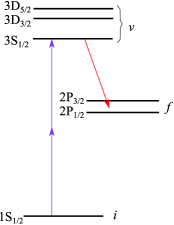
Figure 1: The relevant fine-structure energy levels of hydrogen (I=1/2) or deuterium (I=1).

	Hydrogen		Deuterium
Level	$F$	Freq.(MHz)	$F$	Freq.(MHz)
3S1/2	0	$-39.457$	1/2	$-8.084$
	1	$13.152$	3/2	$4.042$
3D3/2	1	$2927.249$	1/2	$2929.542$
	2	$2931.458$	3/2	$2930.027$
			5/2	$2930.835$
3D5/2	2	$4011.639$	3/2	$4013.498$
	3	$4014.344$	5/2	$4013.844$
			7/2	$4014.329$

Table 1: Energies of the $n=3$ hyperfine sublevels relative to the fine structure 3S_1/2 level, for hydrogen and deuterium. These energy levels were calculated using the NIST database Jentschura et al. (2005) and hyperfine structure data published in Karshenboim and Ivanov (2002). The linewidth $\Gamma_{\nu}/2\pi$ is 1.0 MHz for the 3S level and 10.3 MHz for the 3D levels.

Assuming a near-resonant excitation, this scattering process can be described by an equation of the Kramers-Heisenberg type, similar to eq. (2) of Amaro et al. (2015), in which the excitation operator has been replaced by a two-photon operator :

$$\frac{d\sigma}{d\Omega}\propto\underset{f}{\sum}\left\lvert\underset{\nu}{\sum}~{}\dfrac{Q_{\nu i}(D_{f\nu})^{*}}{\omega_{\nu i}-2\omega-i\Gamma_{\nu}/2}\right\lvert^{2}.$$ (1)

In this equation, $d\sigma/d\Omega$ is the differential cross section of the scattering amplitude, $\omega_{\nu i}$ the transition angular frequency, $\omega$ the laser angular frequency, $Q_{\nu i}$ the matrix element of the two-photon excitation operator, and $D_{f\nu}$ the dipole matrix element corresponding to the one-photon decay.

The cross-damping effect involves transitions from the same initial state ($J_{i}=1/2$, $F_{i}$). For a given $F_{i}$, the sum over $\nu$ can be restricted to the 3S and 3D sublevels allowed by the selection rules Grynberg (1976):
- for the 3S_1/2 level: $F_{\nu}=F_{i}$, due to the selection rule $\Delta F=0$ for two-photon transitions between $J=1/2$ states;
- for the 3D levels: $\Delta F\leq 2$, with $F_{i}=0\to F_{\nu}=1$ and $F_{i}=1/2\to F_{\nu}=1/2$ forbidden.

In the present article, we estimate the cross-damping shift for all possible 1S-3S hyperfine transitions ($F_{i}=0$ and 1 for hydrogen, $F_{i}=1/2$ and 3/2 for deuterium). In our current hydrogen experiment, we study the $F_{i}=1$ transition because the 1S${}_{1/2}^{F=1}$ sublevel is more populated.

II.2 Our experimental situation

We define here the geometry of the scattering process in accordance with our experimental situation. The excitation CW laser at 205 nm is resonant in a Fabry-Perot cavity whose axis is horizontal and collinear with the atomic beam. The laser polarization is vertical. The 3S-2P fluorescence at 656 nm is collected by an imaging system situated directly above the excitation region, and detected by a photo-multiplier. We do not detect the polarization of this fluorescence.

Figure 2 shows the relevant vectors and angles. The two incident photons have the same polarization $\boldsymbol{\varepsilon}_{1}$ (parallel to the $z$ axis), and opposite wave-vectors $\textbf{k}_{1}=-\textbf{k}^{\prime}_{1}$ along the $x$ axis. The wave-vector $\textbf{k}_{2}$ of the scattered photon makes an angle $\theta$ with the vertical $z$ axis, which is chosen as the quantization axis. As mentioned in Brown et al. (2013) and Amaro et al. (2015), the quantum interference effect depends only on this angle $\theta$ between the incident polarization and the scattering direction. Without any loss of generality, we will assume that this wave-vector $\textbf{k}_{2}$ is in the plane $xOz$. We also define $\chi_{2}$ as the angle between the scattered photon’s polarization $\boldsymbol{\varepsilon}_{2}$ and the plane $xOz$.

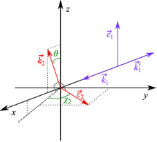
Figure 2: The incident photons have opposite wave-vectors $\textbf{k}_{1}=-\textbf{k}^{\prime}_{1}$ and the same polarization $\boldsymbol{\varepsilon}_{1}$. The direction of the wave-vector $\textbf{k}_{2}$ of the scattered photon defines the angle $\theta$. This photon’s polarization $\boldsymbol{\varepsilon}_{2}$, which lies in a plane perpendicular to $\textbf{k}_{2}$, makes an angle $\chi_{2}$ with the scattering plane $xOz$.

The following calculation is done first in the case of a point-like detector situated at an angle $\theta$ from the $z$ axis. In order to simulate more closely our experimental situation, we will then evaluate the effect for a finite angular aperture of the detection system.

II.3 Details of the calculation

The polarization vectors of the incident ($\boldsymbol{\varepsilon}_{1}$) and scattered ($\boldsymbol{\varepsilon}_{2}$) photons, as defined above, can be written in a spherical basis:

$$\varepsilon_{1}^{(\pm 1)} =0,~{}~{}\varepsilon_{1}^{(0)}=1,$$

$$\varepsilon_{2}^{(\pm 1)} =\mp\dfrac{(\cos\chi_{2}\cos\theta\pm i\sin\chi_{2})}{\sqrt{2}},~{}~{}\varepsilon_{2}^{(0)}=-\cos\chi_{2}\sin\theta.$$ (2)

The dipole matrix element is defined as $D_{f\nu}=\boldsymbol{\varepsilon}_{2}.\textbf{D}_{f\nu}=\langle f|\boldsymbol{\varepsilon}_{2}.\textbf{r}|\nu\rangle$. We can expand the scalar product in the spherical basis, while taking into account the hyperfine structure:

$$D_{F_{f}m_{f}J_{f}}^{F_{\nu}m_{\nu}J_{\nu}}=\underset{\lambda=-1}{\overset{1}{\sum}} (-1)^{\lambda}\varepsilon_{2}^{(-\lambda)}$$ (3)

$$\langle n_{f}L_{f}F_{f}m_{f}J_{f}|r_{\lambda}|n_{\nu}L_{\nu}F_{\nu}m_{\nu}J_{\nu}\rangle.$$

The two-photon matrix element is expressed as:

$$Q_{\nu i} = \left|\underset{r}{\sum}\frac{(\boldsymbol{\varepsilon}_{1}.\textbf{D}_{\nu r})(\boldsymbol{\varepsilon}_{1}.\textbf{D}_{ri})}{\omega-\omega_{ri}}\right|^{2}$$ (4)

$$= \left|\underset{r}{\sum}\frac{\langle\nu|\boldsymbol{\varepsilon}_{1}.\textbf{r}|r\rangle\langle r|\boldsymbol{\varepsilon}_{1}.\textbf{r}|i\rangle}{\omega-\omega_{ri}}\right|^{2}.$$

It can also be written as the matrix element of a $k^{\text{th}}$-order tensor operator $\textsf{{T}}^{(k)}$, with $k=0$ for 1S-3S, $k=2$ for 1S-3D Grynberg (1976). Since the incident polarization $\boldsymbol{\varepsilon}_{1}$ is along the quantization axis (this implies $m_{\nu}=m_{i}$), we simply have:

$$Q_{F_{\nu}m_{\nu}J_{\nu}}^{F_{i}m_{i}J_{i}}=\langle n_{\nu}L_{\nu}F_{\nu}m_{\nu}J_{\nu}|T_{0}^{(k)}|n_{i}L_{i}F_{i}m_{i}J_{i}\rangle.$$ (5)

Defining $\textsf{{T}}^{(1)}=\textbf{r}$, the matrix elements on the right-hand side of eqs. (3) and (5) can be simplified by introducing the reduced matrix element, then successively decoupling the angular momenta to separate radial and angular parts, using the following usual relations Edmonds (1957):

$$\langle n^{\prime}L^{\prime}F^{\prime}m^{\prime}J^{\prime}|T_{\lambda}^{(k)}|nLFmJ\rangle=(-1)^{F^{\prime}-m^{\prime}}\left(\begin{array}[]{ccc}F^{\prime}&k&F\\ -m^{\prime}&\lambda&m\end{array}\right)\langle n^{\prime}L^{\prime}F^{\prime}J^{\prime}||\textsf{{T}}^{(k)}||nLFJ\rangle,$$ (8)

$$\langle n^{\prime}L^{\prime}F^{\prime}J^{\prime}||\textsf{{T}}^{(k)}||nLFJ\rangle=(-1)^{J^{\prime}+I+F+k}\sqrt{[F,F^{\prime}]}\left\{\begin{array}[]{ccc}J^{\prime}&F^{\prime}&I\\ F&J&k\end{array}\right\}\langle n^{\prime}L^{\prime}J^{\prime}||\textsf{{T}}^{(k)}||nLJ\rangle,$$ (11)

$$\langle n^{\prime}L^{\prime}J^{\prime}||\textsf{{T}}^{(k)}||nLJ\rangle=(-1)^{L^{\prime}+S+J+k}\sqrt{[J,J^{\prime}]}\left\{\begin{array}[]{ccc}L^{\prime}&J^{\prime}&S\\ J&L&k\end{array}\right\}\langle n^{\prime}L^{\prime}||\textsf{{T}}^{(k)}||nL\rangle,$$ (14)

with the notation $[J,J^{\prime}]=(2J+1)(2J^{\prime}+1)$. One obtains

$$D_{F_{f}m_{f}J_{f}}^{F_{\nu}m_{\nu}J_{\nu}} =\langle n_{f}L_{f}||\textbf{r}||n_{\nu}L_{\nu}\rangle\times\underset{\lambda=-1}{\overset{1}{\sum}}(-1)^{\lambda}\varepsilon_{2}^{(-\lambda)}A^{f\nu}_{\lambda}(1),$$

$$Q_{F_{\nu}m_{\nu}J_{\nu}}^{F_{i}m_{i}J_{i}} =\langle n_{\nu}L_{\nu}||\textsf{{T}}^{(k)}||n_{i}L_{i}\rangle\times A^{\nu i}_{0}(k),$$ (15)

where we have introduced the angular coefficient $A_{\lambda}(k)$ for a $k^{\text{th}}$-order tensor operator $\textsf{{T}}^{(k)}$:

$$A_{\lambda}(k) =(-1)^{F^{\prime}-m^{\prime}}\left(\begin{array}[]{ccc}F^{\prime}&k&F\\ -m^{\prime}&\lambda&m\end{array}\right)$$ (18)

$$\times (-1)^{J^{\prime}+I+F+k}\sqrt{[F,F^{\prime}]}\left\{\begin{array}[]{ccc}J^{\prime}&F^{\prime}&I\\ F&J&k\end{array}\right\}$$ (21)

$$\times (-1)^{L^{\prime}+S+J+k}\sqrt{[J,J^{\prime}]}\left\{\begin{array}[]{ccc}L^{\prime}&J^{\prime}&S\\ J&L&k\end{array}\right\}.$$ (24)

It should be noted that $A_{0}(0)=1$, as there is no angular coefficient for the 1S-3S excitation.

One can then rearrange the terms to separate radial and angular parts:

$$Q_{F_{\nu}m_{\nu}J_{\nu}}^{F_{i}m_{i}J_{i}}\left(D_{F_{f}m_{f}J_{f}}^{F_{\nu}m_{\nu}J_{\nu}}\right)^{*}=S_{f\nu i}~{}\Omega_{J_{i}J_{\nu}J_{f}}^{F_{i}F_{\nu}F_{f}},$$ (25)

with

$$S_{f\nu i}=\langle n_{f}L_{f}||\textbf{r}||n_{\nu}L_{\nu}\rangle\langle n_{\nu}L_{\nu}||\textsf{{T}}^{(k)}||n_{i}L_{i}\rangle,$$ (26)

$$\Omega_{J_{i}J_{\nu}J_{f}}^{F_{i}F_{\nu}F_{f}}=\underset{m_{\nu},\lambda}{\sum}(-1)^{\lambda}\left(\varepsilon_{2}^{(-\lambda)}\right)^{*}A_{0}(k)A_{\lambda}(1).$$ (27)

Replacing in eq. (1), one obtains:

$$\frac{d\sigma}{d\Omega}\propto\underset{\begin{subarray}{c}F_{f},J_{f},\\ m_{i},m_{f},\boldsymbol{\varepsilon}_{2}\end{subarray}}{\sum}~{}\left\lvert\underset{F_{\nu},J_{\nu}}{\sum}~{}\dfrac{S_{f\nu i}~{}\Omega_{J_{i}J_{\nu}J_{f}}^{F_{i}F_{\nu}F_{f}}}{\omega_{\nu i}-2\omega-i\Gamma_{\nu}/2}\right\lvert^{2}.$$ (28)

It is necessary to sum over $\boldsymbol{\varepsilon}_{2}$ because the polarization of the scattered photon is not detected.

As in Amaro et al. (2015), the terms can be further rearranged to show direct and cross terms:

$$\frac{d\sigma}{d\Omega}\propto\underset{F_{\nu},J_{\nu}}{\sum}\dfrac{S_{f\nu i}^{2}~{}\Lambda_{J_{i}J_{\nu}}^{F_{i}F_{\nu}}}{(\omega_{\nu i}-2\omega)^{2}+(\Gamma_{\nu}/2)^{2}}~{}+~{}\text{Re}\left[\underset{(F^{\prime}_{\nu},J^{\prime}_{\nu})>(F_{\nu},J_{\nu})}{\sum}\dfrac{S_{f\nu i}~{}S_{f\nu^{\prime}i}~{}\Xi_{J_{i}J_{\nu}J_{\nu^{\prime}}}^{F_{i}F_{\nu}F_{\nu^{\prime}}}}{(\omega_{\nu i}-2\omega-i\Gamma_{\nu}/2)(\omega_{\nu^{\prime}i}-2\omega+i\Gamma_{\nu^{\prime}}/2)}\right]$$ (29)

where we have defined

$$\Lambda_{J_{i}J_{\nu}}^{F_{i}F_{\nu}}=\underset{\begin{subarray}{c}F_{f},J_{f},\\ m_{i},m_{f},\boldsymbol{\varepsilon}_{2}\end{subarray}}{\sum}\left|\Omega_{J_{i}J_{\nu}J_{f}}^{F_{i}F_{\nu}F_{f}}\right|^{2}~{}~{}~{}\text{and}~{}~{}~{}\Xi_{J_{i}J_{\nu}J_{\nu^{\prime}}}^{F_{i}F_{\nu}F_{\nu^{\prime}}}=2\text{Re}\left[\underset{\begin{subarray}{c}F_{f},J_{f},\\ m_{i},m_{f},\boldsymbol{\varepsilon}_{2}\end{subarray}}{\sum}\Omega_{J_{i}J_{\nu}J_{f}}^{F_{i}F_{\nu}F_{f}}\left(\Omega_{J_{i}J_{\nu^{\prime}}J_{f}}^{F_{i}F_{\nu^{\prime}}F_{f}}\right)^{*}\right].$$ (30)

II.4 Radial part

The two matrix elements in eq. (26) can be evaluated in the following way.

$\langle n_{f}L_{f}||\textbf{r}||n_{\nu}L_{\nu}\rangle$ is the well-known reduced matrix element of the radial operator r and can be easily calculated using the Wigner-Eckart theorem:

$$\langle nLm| r_{\lambda}| n^{\prime}L^{\prime}m^{\prime}\rangle$$ (33)

$$= (-1)^{L-m}\left(\begin{array}[]{ccc}L&1&L^{\prime}\\ -m&\lambda&m\end{array}\right)\langle nL||\textbf{r}||n^{\prime}L^{\prime}\rangle.$$

For example, defining $\psi_{nLm}$ as the usual electronic wave function of hydrogen, one has:

$$\langle 2\text{P}0|z|3\text{D}0\rangle = (-1)^{1-0}\left(\begin{array}[]{ccc}1&1&2\\ 0&0&0\end{array}\right)\langle 2\text{P}||\textbf{r}||3\text{D}\rangle$$ (36)

$$= \int\psi_{210}^{*}(r)~{}z~{}\psi_{320}(r)~{}d^{3}r,$$ (37)

where the integral is calculated over the whole space.

The two-photon matrix element has been calculated by M. Haas et al. Haas et al. (2006). It is given by:

$$\langle n_{\nu}L_{\nu}||\textsf{{T}}^{(k)}||n_{i}L_{i}\rangle=-\frac{2hc\epsilon_{0}}{e^{2}}\times\beta_{ge}^{(k)},$$ (38)

where the coefficients $\beta_{ge}^{(k)}=\beta_{ge}$ for 1S-3S and $\beta_{ge}^{(2)}$ for 1S-3D are given in tables II and III of Haas et al. (2006). These coefficients are given in Hz(W/m²)^-1.

In our case, the radial part is

$$\langle 3\text{S}||\textsf{{T}}^{(0)}||1\text{S}\rangle=1.00333\times C,$$

$$\langle 3\text{D}||\textsf{{T}}^{(2)}||1\text{S}\rangle=-6.16579\times C,$$

$$\langle 2\text{P}||\textbf{r}||3\text{S}\rangle=0.938404\times a_{0},$$

$$\langle 2\text{P}||\textbf{r}||3\text{D}\rangle=-6.71467\times a_{0},$$ (39)

where $C=-10^{-5}\times\frac{2hc\epsilon_{0}}{e^{2}}$ and $a_{0}$ is the Bohr radius. Both constants are global factors and we do not take them into account.

In the numerical calculations, we then simply used:

$$S_{f\nu i}=\left\{\begin{array}[]{cc}1.00333\times 0.938404&\text{for }\nu=\text{3S}\\ -6.16579\times(-6.71467)&\text{for }\nu=\text{3D}\end{array}\right.$$ (40)

II.5 Angular part

As noted earlier, the quantum interference effect depends only on the angle $\theta$ between the incident polarization and the scattering direction. Hence, the coefficients $\Lambda$ and $\Xi$ have a simple angular dependence and can be parametrized as follows:

$$\Lambda_{J_{i}J_{\nu}}^{F_{i}F_{\nu}}(\theta)=a_{0}+a_{2}P_{2}(\cos\theta),$$

$$\Xi_{J_{i}J_{\nu}J_{\nu^{\prime}}}^{F_{i}F_{\nu}F_{\nu^{\prime}}}(\theta)=b_{2}P_{2}(\cos\theta),$$ (41)

where $P_{2}$ is the second-order Legendre polynomial: $P_{2}(x)=(3x^{2}-1)/2$.

Table 2 gives the coefficients of this parametrization for hydrogen: direct terms for each hyperfine transition, and cross terms between the 1S-3S transition and the 1S-3D transitions. In deuterium, the hyperfine structure is different but the method developed above can be directly applied: the radial part is the same (eq. (40)), and the angular part should be changed accordingly (Table 3).

The cross terms between 3D levels play a negligible role in the distortion and shifting of the 1S-3S line. They are not included in these tables but are given in the Appendix.

$F_{i}$	$L_{\nu}$	$F_{\nu}$	$J_{\nu}$	$a_{0}$	$a_{2}$	$b_{2}$
0	0	1	1/2	2/3	0
	2	2	3/2	4/375	-7/1875	$4\sqrt{2}/75$
	2	2	5/2	2/125	-4/625	$2\sqrt{2}/25$
1	0	1	1/2	2	0
	2	1	3/2	2/125	-7/2500	$2\sqrt{2}/25$
	2	2	3/2	2/125	-7/2500	$2\sqrt{2}/25$
	2	2	5/2	4/375	-4/1875	$4\sqrt{2}/75$
	2	3	5/2	14/375	-8/625	$14\sqrt{2}/75$

Table 2: Angular coefficients for hydrogen, $F_{i}=0$ and 1.

$F_{i}$	$L_{\nu}$	$F_{\nu}$	$J_{\nu}$	$a_{0}$	$a_{2}$	$b_{2}$
1/2	0	1/2	1/2	4/3	0
	2	3/2	3/2	8/1875	-14/46875	$8\sqrt{2}/375$
	2	5/2	3/2	32/1875	-224/46875	$32\sqrt{2}/375$
	2	3/2	5/2	32/1875	-224/46875	$32\sqrt{2}/375$
	2	5/2	5/2	28/1875	-184/46875	$28\sqrt{2}/375$
3/2	0	3/2	1/2	8/3	0
	2	1/2	3/2	4/375	0	$4\sqrt{2}/75$
	2	3/2	3/2	32/1875	0	$32\sqrt{2}/375$
	2	5/2	3/2	28/1875	-14/9375	$28\sqrt{2}/375$
	2	3/2	5/2	8/1875	0	$8\sqrt{2}/375$
	2	5/2	5/2	32/1875	-436/459375	$32\sqrt{2}/375$
	2	7/2	5/2	16/375	-16/1225	$16\sqrt{2}/75$

Table 3: Angular coefficients for deuterium, $F_{i}=1/2$ and 3/2.

III Results

In order to estimate the frequency shift due to the cross-damping effect, we calculate a simulated signal taking into account the direct and cross terms using eq. (29). We then fit the 1S-3S line with a simple Lorentzian function, leaving all fit parameters (position, width, amplitude) free. The shift is defined here as the difference between the position given by the fit and the theoretical position used in the calculation.

We do not add any noise to the simulated spectrum; in our experiment, there is a rather large background so the noise can be approximated by a white noise. We have checked that adding a white noise to the simulated signal does not significantly change the result of the fit.

III.1 Point-like detector

Figure 3(a) shows the simulated signal for hydrogen, $F_{i}=1$, in the case of a point-like detector situated directly above the excitation point ($\theta=0$). The second term on the right-hand side of eq. (29) is the signature of quantum interference, and is represented in Fig. 3(b). Its dispersion shape is responsible for the shift of the transition frequency. All the results given below are shifts of the laser frequency $\omega/2\pi$, and differ from the atomic transition frequency shifts by a factor of two.

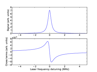
Figure 3: (a) Simulated 1S-3S signal for hydrogen, $F_{i}=1$, $\theta=0$. (b) Sum of the cross terms; the arbitrary units are the same as in (a), but the vertical scale is amplified by a factor of 500.

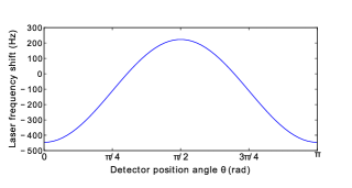
Figure 4: Shift of the laser frequency as a function of detector position angle $\theta$.

Figure 4 shows the frequency shift as a function of the position of a point-like detector. The shift is maximal for $\theta=0$, and is proportional to $P_{2}(\cos\theta)$, having the same angular dependence as the amplitude of the cross terms. This fact is not surprising, since the shift is very small compared to the natural linewidth, and can be expected to vary linearly with the amplitude of the cross terms.

This figure is comparable to the results of D. Yost et al. (Fig. 5 of Yost et al. (2014)), that were calculated using a completely different method in which the continuous excitation was treated as a special case.

	$F_{i}$	Shift (Hz)
H	0	$-$440
	1	$-$446
D	1/2	$-$444
	3/2	$-$445

Table 4: Calculated shift for $\theta=0$, in Hz.

Table 4 gives the maximal shift, calculated for $\theta=0$, for the four possible hyperfine transitions. It is interesting to notice that we find very similar shifts for the different cases. This is due to the fact that the hyperfine structure of the 3D levels is not resolved because it is smaller than the natural linewidth of these levels. The frequency shift is thus at most of $-$0.45 kHz for all 1S-3S transitions; we also find this result if we ignore the hyperfine structure in the calculations.

One can also compare this shift to a naive estimate derived from the simplified case of a three-level atom. The calculation of the first term in eq. (25) of Horbatsch and Hessels (2010) would give, with $\Gamma=1$ MHz and $\Delta\approx 3000$ MHz:

$$\Gamma^{2}/4\Delta\approx 0.08~{}\rm kHz.$$ (42)

In fact, this gives the atomic frequency shift due to a single cross term between excited levels of linewidth $\Gamma$ and separated by $\Delta$, assuming that the cross term and direct term have the same amplitude. In our case, there are several cross-terms, and as we can see in eq. (29), these cross terms all have different amplitudes; thus, we should take into account the amplitude ratio between each cross term and the direct term, and sum over all 3D sublevels $\nu^{\prime}$ interfering with the 3S level $\nu$, in order to calculate the total atomic frequency shift:

$$\delta(2\omega)\approx\underset{\nu^{\prime}}{\sum}\left[\frac{\Gamma_{\nu}^{2}}{4(\omega_{\nu i}-\omega_{\nu^{\prime}i})}\times\frac{S_{f\nu^{\prime}i}\times\Xi_{J_{i}J_{\nu}J_{\nu^{\prime}}}^{F_{i}F_{\nu}F_{\nu^{\prime}}}(\theta)}{S_{f\nu i}\times\Lambda_{J_{i}J_{\nu}}^{F_{i}F_{\nu}}}\right].$$ (43)

For $\theta=0$, this equation gives $\delta(2\omega)\approx-0.45$ kHz, which is indeed a very good estimate of the shift.

III.2 Extended detector

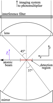
Figure 5: Side view of the fluorescence collection system.

In order to simulate more closely our experiment, we can integrate the signal over the angular aperture of our imaging system. The point-like detector case for $\theta=0$ gives an upper bound for the frequency shift; any integration over this angle will only reduce the effect. Furthermore, integrating over the whole space cancels the effect altogether.

The fluorescence collection system is shown in Fig. 5. The scattered photons are collected through an aspheric lens of radius 25 mm and an interference filter at 656 nm. A spherical metallic mirror, having the same radius as the lens and situated below the excitation region, increases the solid angle of detection by redirecting photons emitted downwards. The 10^∘ acceptance angle of the interference filter limits the length of the detection region along the atomic beam, which is then a segment of length 12 mm centered on the waist of the 205 nm Fabry-Perot cavity. The center of this detection region is the focal point of the lens as well as the center of curvature of the spherical mirror.

Let us assume for now that the detection region is infinitesimal and centered: in this situation, only photons emitted at the center of the cavity are detected. We can first integrate the simulated signal over the upper part of the collection system:

$$Signal=\int_{0}^{\theta_{max}}f(\theta)\times 2\pi\sin(\theta)d\theta,$$ (44)

where $f(\theta)$ is the right-hand side of eq. (29), and $\theta_{max}$ is the half angle of the detection cone. With $\theta_{max}=45^{\circ}$ defined by the diameter of the lens, equation (44) leads to a laser frequency shift of $-$0.27 kHz.

Then, it is possible to calculate the signal for a given position of the emission point along the detection region. The angular acceptance of the filter can be approximated by a step function of the incident angle, so that the distribution of the emission points is assumed to be uniform along the segment. Integrating over the length of the detection region does not change the result significantly ($<$1 Hz).

We can thus simply add to the previous signal of eq. (44) the integral over the downwards-emitted photons reflected by the spherical mirror, with an opening half- angle of 37^∘, neglecting the losses due to the reflection on the mirror:

$$Signal=\int_{0}^{45^{\circ}} f(\theta) \times 2\pi\sin(\theta)d\theta$$ (45)

$$+ \int_{0}^{37^{\circ}}f(\theta)\times 2\pi\sin(\theta)d\theta.$$

This results in a frequency shift of $-$0.29 kHz.

IV Conclusion

In this article, we have estimated the frequency shift, due to the cross-damping effect, of the 1S-3S transition of hydrogen and deuterium, in the conditions of the experiment in progress in our group. This shift is similar for both isotopes, and depends on the angle at which the fluorescence photon is emitted with respect to the polarization of the incident laser light. The maximal shift of the laser frequency is of $-$0.45 kHz, assuming a point-like detector situated at the vertical of the excitation point. After taking into account the actual geometry of our detection system, we found a laser frequency shift of $-$0.29 kHz. This corresponds to a shift of the atomic frequency of $-$0.58 kHz, that is smaller than the current statistical uncertainty (2.2 kHz Galtier et al. (2015)) of our measurements.

*

Appendix A

Tables 5 and 6 present the coefficient $b_{2}$, as defined in eq. (41), for the cross terms between the different 3D hyperfine sublevels. These cross terms do not play any significant role in shifting the 1S-3S line.

$F_{i}$	$F_{\nu}$	$J_{\nu}$	$F_{\nu^{\prime}}$	$J_{\nu^{\prime}}$	$b_{2}$
0	2	3/2	2	5/2	-2/625
1	1	3/2	2	3/2	-7/1250
	1	3/2	2	5/2	-7/1875
	1	3/2	3	5/2	-2/1875
	2	3/2	2	5/2	1/625
	2	3/2	3	5/2	-4/625
	2	5/2	3	5/2	-8/1875

Table 5: Angular coefficients of cross terms between 3D sublevels of hydrogen.

$F_{i}$	$F_{\nu}$	$J_{\nu}$	$F_{\nu^{\prime}}$	$J_{\nu^{\prime}}$	$b_{2}$
1/2	3/2	3/2	5/2	3/2	-112/46875
	3/2	3/2	3/2	5/2	-112/46875
	3/2	3/2	5/2	5/2	52/46875
	5/2	3/2	3/2	5/2	-16/15625
	5/2	3/2	5/2	5/2	-64/15625
	3/2	5/2	5/2	5/2	-64/15625
3/2	1/2	3/2	3/2	3/2	-56/9375
	1/2	3/2	5/2	3/2	-14/9375
	1/2	3/2	3/2	5/2	-14/9375
	1/2	3/2	5/2	5/2	-16/9375
	1/2	3/2	7/2	5/2	0
	3/2	3/2	5/2	3/2	-56/9375
	3/2	3/2	3/2	5/2	0
	3/2	3/2	5/2	5/2	-208/65625
	3/2	3/2	7/2	5/2	-128/65625
	5/2	3/2	3/2	5/2	2/3125
	5/2	3/2	5/2	5/2	32/21875
	5/2	3/2	7/2	5/2	-144/21875
	3/2	5/2	5/2	5/2	-64/21875
	3/2	5/2	7/2	5/2	-32/65625
	5/2	5/2	7/2	5/2	-1152/153125

Table 6: Angular coefficients of cross terms between 3D sublevels of deuterium.

References

- Pohl et al. (2013) R. Pohl, R. Gilman, G. A. Miller, and K. Pachucki, Annu. Rev. Nucl. Part. Sci. 63, 175 (2013).
- Carlson (2015) C. E. Carlson, Prog. Part. Nucl. Phys. 82, 59 (2015).
- Horbatsch and Hessels (2010) M. Horbatsch and E. A. Hessels, Phys. Rev. A 82, 052519 (2010).
- Brown et al. (2013) R. C. Brown, S. Wu, J. V. Porto, C. J. Sansonetti, C. E. Simien, S. M. Brewer, J. N. Tan, and J. D. Gillaspy, Phys. Rev. A 87, 032504 (2013).
- Amaro et al. (2015) P. Amaro, B. Franke, J. J. Krauth, M. Diepold, F. Fratini, L. Safari, J. Machado, A. Antognini, F. Kottmann, P. Indelicato, R. Pohl, and J. P. Santos, Phys. Rev. A 92, 022514 (2015).
- Beyer et al. (2015) A. Beyer, L. Maisenbacher, K. Khabarova, A. Matveev, R. Pohl, T. Udem, T. W. Hänsch, and N. Kolachevsky, Physica Scripta T165, 014030 (2015).
- Yost et al. (2016) D. C. Yost, A. Matveev, A. Grinin, E. Peters, L. Maisenbacher, A. Beyer, R. Pohl, N. Kolachevsky, K. Khabarova, T. W. Hänsch, and T. Udem, Phys. Rev. A 93, 042509 (2016).
- Galtier et al. (2015) S. Galtier, H. Fleurbaey, S. Thomas, L. Julien, F. Biraben, and F. Nez, J. Phys. Chem. Ref. Data 44, 031201 (2015).
- Yost et al. (2014) D. C. Yost, A. Matveev, E. Peters, A. Beyer, T. W. Hänsch, and T. Udem, Phys. Rev. A 90, 012512 (2014).
- Jentschura et al. (2005) U. Jentschura, S. Kotochigova, E. LeBigot, P. Mohr, and B. Taylor, The Energy Levels of Hydrogen and Deuterium (version 2.1) (National Institute of Standards and Technology, Gaithersburg, MD, 2005) available at http://physics.nist.gov/HDEL .
- Karshenboim and Ivanov (2002) S. G. Karshenboim and V. G. Ivanov, Eur. Phys. J. D 19, 13 (2002).
- Grynberg (1976) G. Grynberg, Thèse de doctorat d’Etat, Université Pierre et Marie Curie (1976), available at https://tel.archives-ouvertes.fr/tel-00011825 .
- Edmonds (1957) A. R. Edmonds, Angular momentum in quantum mechanics (Princeton University Press, Princeton, NJ, 1957).
- Haas et al. (2006) M. Haas, U. D. Jentschura, C. H. Keitel, N. Kolachevsky, M. Herrmann, P. Fendel, M. Fischer, T. Udem, R. Holzwarth, T. W. Hänsch, M. O. Scully, and G. S. Agarwal, Phys. Rev. A 73, 052501 (2006).