The topological face of recommendation:
models and application to bias detection

Abstract

Recommendation plays a key role in e-commerce and in the entertainment industry. We propose to consider successive recommendations to users under the form of graphs of recommendations. We give models for this representation. Motivated by the growing interest for algorithmic transparency, we then propose a first application for those graphs, that is the potential detection of introduced recommendation bias by the service provider. This application relies on the analysis of the topology of the extracted graph for a given user; we propose a notion of recommendation coherence with regards to the topological proximity of recommended items (under the measure of items’ $k$-closest neighbors, reminding the ”small-world” model by Watts & Stroggatz). We finally illustrate this approach on a model and on Youtube crawls, targeting the prediction of ”Recommended for you” links (i.e., biased or not by Youtube).

The output of recommender systems are benchmarked by researchers and practitioners based on their precision and recall performances on test datasets [11]. Yet, while those metrics have proven useful for assessing the performances of recommenders, we find that the graph data-structure has not been applied for studying and learning about the recommendations made to users (i.e., the recommenders’ outputs). We argue that graph theory and the wide spectrum of graph algorithms available for data mining complex networks can be as well leveraged for complementing studies about recommender results. Our proposal is to represent the recommendations to users in either a global graph of recommendations, available by the service provider at a given point in time, or as a user-graph of recommendations that only captures the recommendation space to a single user, and that can also be observed at the service or by the user herself through the crawling of the service recommendation interface. The extracted graph topology is thus to be leveraged for analysis.

One application we target is related to the field of algorithmic transparency. Some major service providers, such as Youtube, comment on the high level implementation of their recommender, without specifying details that would allow a transparent use by the public [4]. Recently, there has been an increase in the will for accountability of the service provided by those systems, that can be viewed as black-boxes operating in the cloud, and that a user interacts with by providing her profile or by calling API operations [8, 9, 13]. In the setup of the observation by a user of what she gets as recommendations, both the input (her user profile) and the output (tens of recommendations) are very sparse in comparison to the dataset belonging to the service provider for analysis. In this paper, we show as an application that observed user-graphs of recommendations, despite their sparsity, bring interesting learning.

We first illustrate in next section the construction of a user-graph of recommendations.

1 Illustration: user’s recommendations as a graph

Recommendations on a website take the simple form of a set of displayed items, for the user to interact with. We propose to go beyond the collection of this flat item-set, by crawling from each proposed item, recursively, up to a limited depth $h$ (for obvious practical reasons). On the canonical example of crawling from an item web-page (e.g., video), where $k$ other related items are recommended, and where each item is only recommended once in total, we would obtain a balanced tree of $n_{tree}^{h}(k)=\frac{k^{h+1}-1}{k-1}$ nodes.

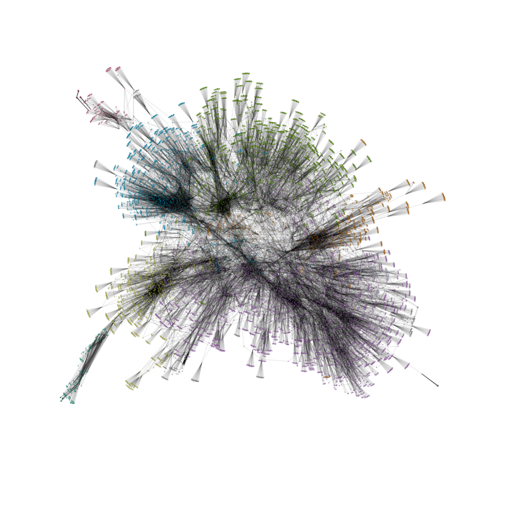
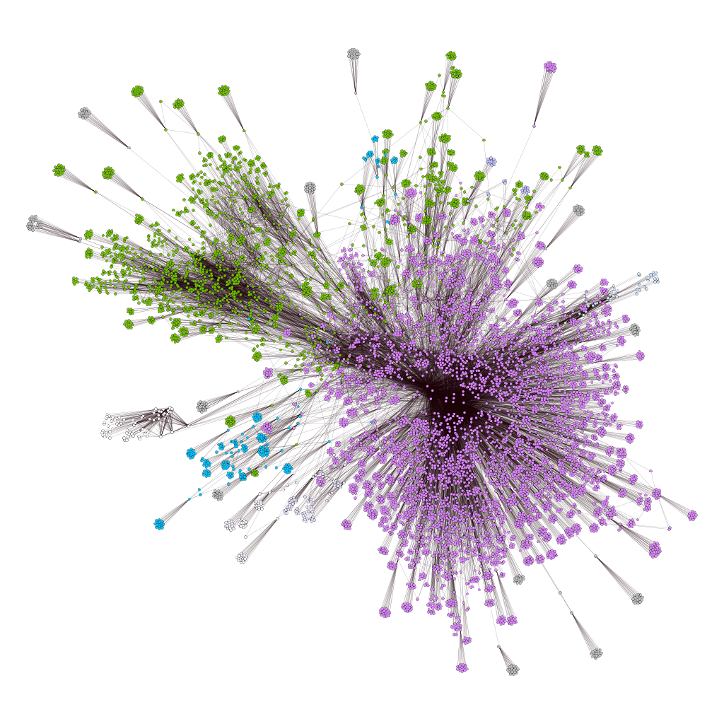
Figure 1: 4-hops recommendation graphs from a Youtube video, new user (left) and returning user (right).

We use the example of video recommendation in this paper. In the mainstream Youtube platform, we start crawling recommended video web-pages from a given video (a popular one from Lady Gaga), with $h=4$. The crawling does not appear to be rate-limited, so we could collect tens of thousands of web-pages in the order of a minute. We remark that 19 videos are recommended at each page ($k=19$). There are two clear modes of video viewing in such a system; (i) case $\bcancel{\mathcal{C}}$: a user is new to the platform, or (ii) $\mathcal{C}$: she is a returning user, and thus has a history on it (recognized by Youtube through the passing of a cookie by our web-crawler). Drastic differences occur when building the graphs for both scenario (the two crawls are separated by only few seconds); $\bcancel{\mathcal{C}}$: $n_{\bcancel{\mathcal{C}}}^{4}(19)=14,121$ nodes and has $36,435$ edges. In case $\mathcal{C}$, $n_{\mathcal{C}}^{4}(19)=8,786$ nodes and has $24,731$ edges. Both graphs are displayed on Figure 1. First observation is that as $n_{tree}^{4}(19)=137,561$, there is a high redundancy of recommendations, within both $\bcancel{\mathcal{C}}$ and $\mathcal{C}$. Very interestingly, crawl $\mathcal{C}$ contains around $38\%$ less nodes than $\bcancel{\mathcal{C}}$. This has to be interpreted by the recommender system “knowing” the user, and then trying at each video access to insist in the recommendation of what it thinks is best suited for that user to enjoy. In case $\bcancel{\mathcal{C}}$ (new user), the recommender presents videos related to the start one as well, but also includes in its recommendations videos from different categories (sport, news, …), in the probable hope to gain knowledge faster about the user by varying its propositions. Those phenomenons are confirmed by analyzing graph structures: a search for main clustered components (through the modularity algorithm with $p=5.0$) indicates $7$ components of size at least $1\%$ of the graph size for graph from $\bcancel{\mathcal{C}}$, versus only $3$ for case $\mathcal{C}$ (i.e., more precise recommendations lead to fewer clusters of interest for the returning user). Node colors corresponds to components they belong to, on Figure 1. Another key difference is the degree distribution, with $3$ nodes having more than $100$ in-neighbors for $\bcancel{\mathcal{C}}$, versus $10$ in the second case: videos assumed relevant by the system are consistently recommended to the returning user.

An immediate conclusion drawn from the structural analysis of both $\bcancel{\mathcal{C}}$ and $\mathcal{C}$ graphs, is that their topological comparison informs about the degree of knowledge of the system about the observing user, even under a limited exploration scope. Having illustrated the possibility for a user to crawl a recommender system and analyze its output under the form of a graph of recommendations, we now define two variants of a general graph model for analyzing recommendations.

2 Representation for graphs of recommendations

The aim of recommendation is to propose suited items to users, in the global set of available items, and based on the freshest information available for those users. We focus for this model on item-item recommendation [11], i.e., other items that are presented to a user enjoying or reviewing a given item.

Let’s imagine the service provider taking a snapshot of the recommender’s system data-structures, so that all operations on those data-structures are frozen and observable at arbitrary time $t$. From such a snapshot, the recommendations for a given user-item tuple $\langle u,i\rangle$, provided by an arbitrary recommendation algorithm, are observable or computable under the form of e.g., a ranked list of items.

Definition 2.1 (Graph of recommendations).

The directed graph $G_{t}=(V_{t},E_{t},W_{t})$ is extracted at time $t$, with $V_{t}$ the set of available items (nodes), $E_{t}$ the set of edges (i.e., the recommendations) connecting some nodes from $V_{t}$, and $W_{t}$ the weight of those edges (i.e., their number of occurrences). Edges are thus $E_{t}\subseteq V_{t}\times V_{t}$, and gathered from the system data-structures as the union of recommendation lists for every user from user set $U_{t}$, at time $t$: $E_{t}=\cup^{u\in U_{t},i\in V_{t}}\langle u,i\rangle$.

The recommender system’s working internals, adapting to the inherent data and user churn on the platform as the time passes by, are triggering changes on the graph to be observed.

We now introduce the user-centric counterpart of Definition 2.1:

Definition 2.2 (User-graph of recommendations).

The directed graph $G_{t}(u)=(V_{t},E_{t})$ is extracted at time $t$, using the same data-structures as in Definition 2.1, with the restriction to recommendations to a single given user $u$: $E_{t}=\cup^{u,i\in V_{t}}\langle u,i\rangle$.

$G_{t}$ from Definition 2.1 is of interest for service providers, for instance for estimating user flows among the proposed videos (e.g., such as in the random surfer model over web-pages linked as a graph [2]), while $G_{t}(u)$ from Definition 2.2 is of interest for a user observation of her recommendation outputs (as discussed in the paper sequel).

The dynamics of graphs of recommendations

While snapshotting data-structures to build $G_{t}$ or $G_{t}(u)$ (i.e., for a target user $u$) is expected to be relatively straightforward for service operators with full control over their recommender system (even in the context of distributed data-structures [1]), this is more complex for an external observer such as a user of a platform proposing recommendations.

The observation by a user $u$ of her user-graph of recommendation may e.g., be conducted through the platform API or by a crawling the service interface (as exposed in Section 1). Because item/user churn and recommendation computation on a large platform is expected to occur quickly, and because a crawl is in essence a sequential operation, such an observation may differ from a system snapshot $G_{t}(u)$: (i) clearly, the worst case for an observer is when in between the access to two items, the system has updated its recommendations, thus possibly triggering another state for the user-graph of recommendations. (ii) Yet, for practical implementation reasons of the recommender service (most notably recommendation latency), batch-oriented pre-computations are implemented, rather than on-demand computation of recommendations [5]; this means that recommendations are updated for instance few times a day, which leaves the observer with a more stable system to observe. We assume such a practical scenario for our application based on observations, in the sequel of this paper.

Definition 2.3 (Observed user-graph of recommendations).

$\hat{G}_{t}^{h}(u,i)$ denotes a user observation of $G_{t}(u)$, where $t$ is indicating the arbitrary time at which the first item $i$ is collected to sequentially build the user-graph of recommendations, and $h$ is the depth of exploration away from $i$.

The aim of the observer is thus to collect an observation as close as possible from a snapshot, by e.g., collecting a $\hat{G}_{t}^{h}(u,i)$ with a small $h$ (thus referring to a local observation around the initial item $i$, minimizing access to other items), and as quickly as possible to mitigate recommendation re-computations. In practice, this is the data we gather in Section 2 by using a web-crawler.

3 An application for graphs of recommendations: detecting recommendation bias with topology

A recently discussed topic is the influence of online medias, and their capacity to shape opinion and user tastes based on item recommendations. We propose a technical approach based on user-graphs of recommendations for this question.

Recommender Model

We consider recommenders that, given an item $i\in V_{t}$ long with some other type of information like the user profile) return a score $s_{R}^{i}:V_{t}\mapsto[0,1]$ typically capturing items similar to $i$ [11]. The output of such a recommender system $R$ is then exploited by a service that selects the subset of best matching items that will get recommended when a user $u$ consults $i$ (typically a ranking operation, as exposed in [4]). Let $R_{i}(u)\subset V_{t}$ be this set of recommended items to $u$ at a web-page: $\forall j\in R_{i}(u),j^{\prime}\in V_{t}\setminus R_{i}(u),s_{R}^{i}(u,j)\geq s_{R}^{i}(u,j^{\prime})$. By selecting a recommended item $j\in R_{i}(u)$, $u$ enjoys $j$, and in turn gets recommended items similar to $j$, namely $R_{j}(u)$.

In this context, the user-graph of recommendations (Definition 2.2) for $u$ is $G_{t}(u)$, in which an edge $(i,j)\in E_{t}\Leftrightarrow j\in R_{i}(u)$, at time $t$. In a system that biases recommendations, the user is proposed certain items (for economical, or legal reasons for instance): this translates in biased edges toward items from set $V_{t}$.

Bias in an observed user-graph of recommendations

The service officially exploits the recommender $R$ (such as the one advertised in  [4]). The service may add recommendation bias in destination to user $u$ for orienting her navigation among items; this translates into $G_{t}(u)$ containing biased edges. Let $E_{t,B}$ this set of biased edges; we thus have $G_{t}(u)=(V_{t},E_{t}\cup E_{t,B})$, observed as $\hat{G}_{t}^{h}(u,i)$.

We now ask the following question: having access to $\hat{G}_{t}^{h}(u,i)$, can user $u$ decide whether a given edge of that graph is biased or not? Hereafter, we propose a model for addressing this question, that is based on the small-world parallel with graphs of recommendations.

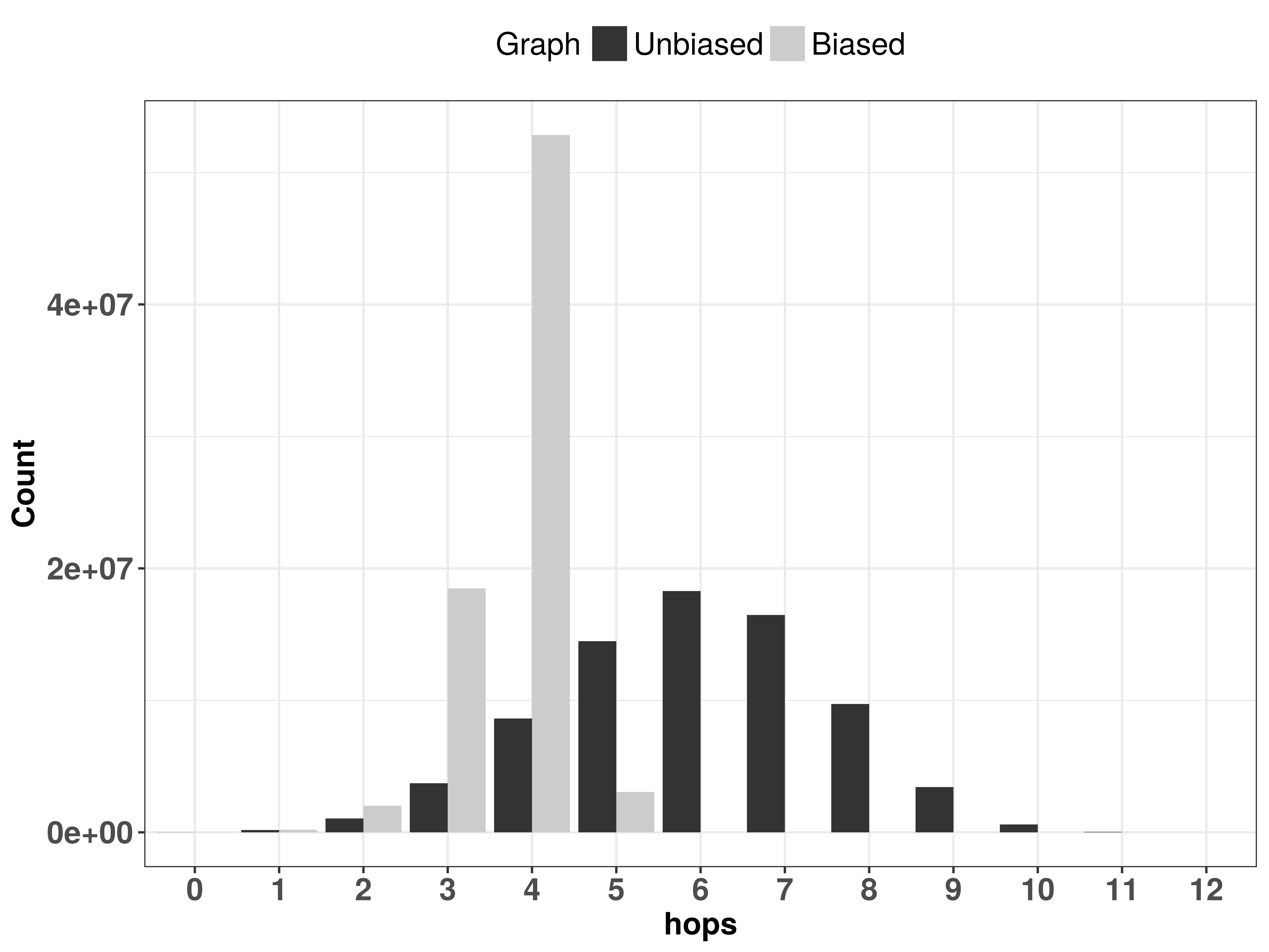
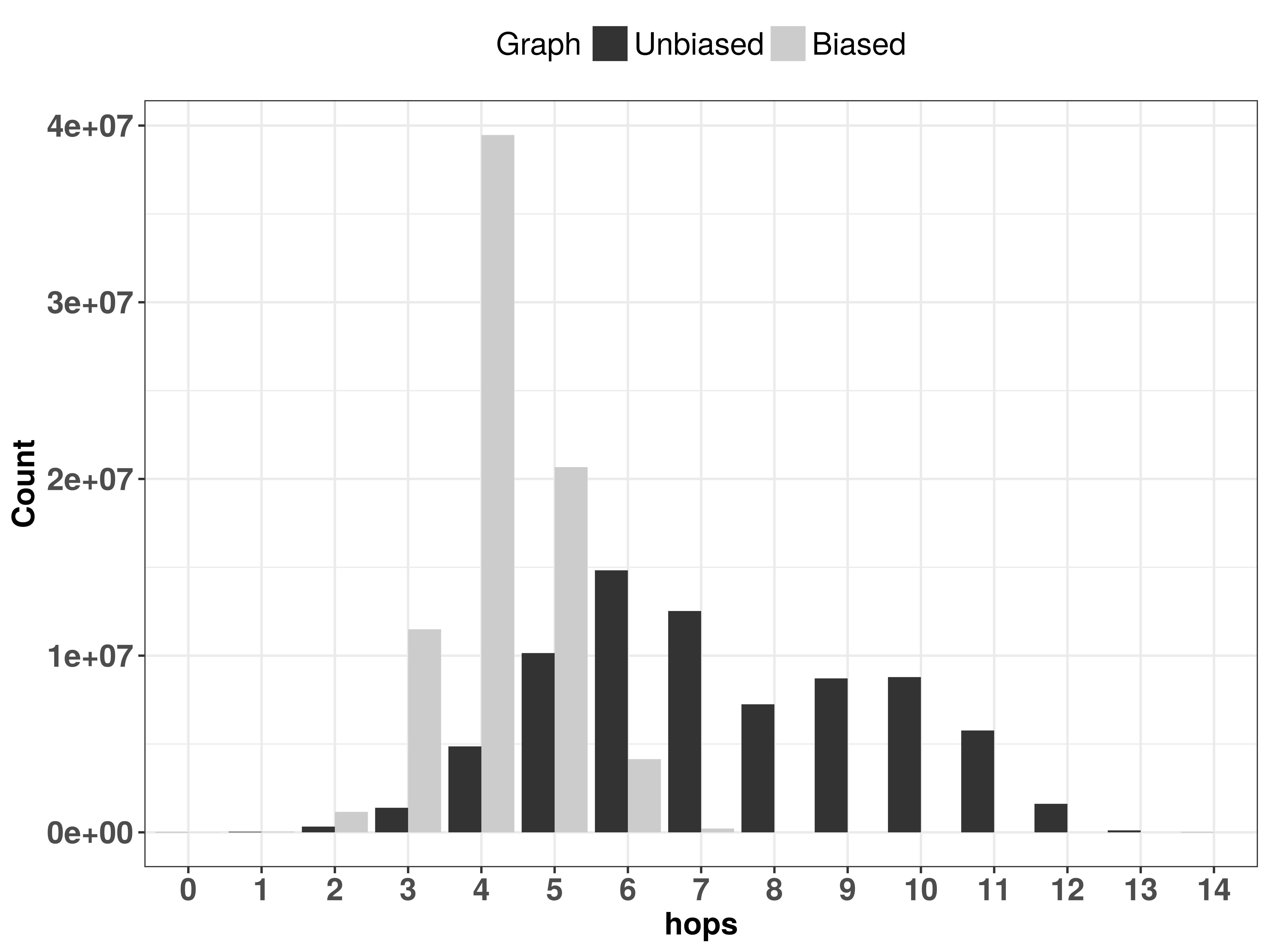
Figure 2: Distribution of graph path lengths for the experiments: model (left) and a Youtube crawl (right).

3.1 Towards algorithms for tagging long biased edges

We propose to study potential bias in recommendation graphs, in relation to the locality or not of recommended items. For avoiding a formal - and possibly debatable - definition of bias, we instead state two of its most probable topological consequences on user-graph of recommendations $\hat{G}_{t}(u,i)$:
Proposition 1 Biased edges impact graph structure: if the service bothers to bias recommendations to a user, it is because it effectively impacts that user navigation among items. That is, users do not navigate the same way in an unbiased graph than in a graph $G_{t}(u)$ containing biased edges. Therefore, the existence of biased edges must significantly change the properties of the observed graph.
Proposition 2 Recommenders leverage item proximity, and this appears in a graph observation: most of recommenders exploit some underlying coherence among the items. Collaborative filtering exploits correlations in users’ tastes: if users enjoying $a$ also usually enjoy $b$, $b$ will be recommended from $a$ and vice versa [11]. This symmetry translates into edge locality in $G_{t}(u)$, captured by e.g., clustering (as appearing through clusters on Figure 1). Biased edges might not rely on such property, and therefore are less likely to produce locality. We also can argue that if bias actually results in the proposal of usual (i.e., local) items for a user, she is not likely to consider those recommendations as biased.

In practice, machine learning algorithms associate to each item a $d$-dimensional vector of features; a recommender then for instance rely on $k$ nearest neighbors ($k$NN) or cosine similarity on those vectors. Recommended items are thus often close-by in the $d$-dimensional feature space, while we expect biased edges to point to items that are relatively far in the feature space. Note that this observation of the effect of biased edges on the topology may relate to services providing serendipitous recommendations [11] (for bringing diversity to a user); this nevertheless arguably constitutes a form of bias w.r.t. user habits.

A small-world perspective

We now propose to identify bias using a parallel to the Watts-Strogatz “small-world” model [14]. In that model, nodes have local connectivity in a given space between them (capturing for instance a geographical proximity), but also have so called long-range links (capturing for instance a familial relationship, loosely related to a geographical proximity). The consequences of these long edges are well known: they drastically impact average path length. We argue that biased links added to the recommender output have the same impact: provided they are different enough from the recommender edges, they will impact the graph structure. To capture this degree of difference, we propose the following model:

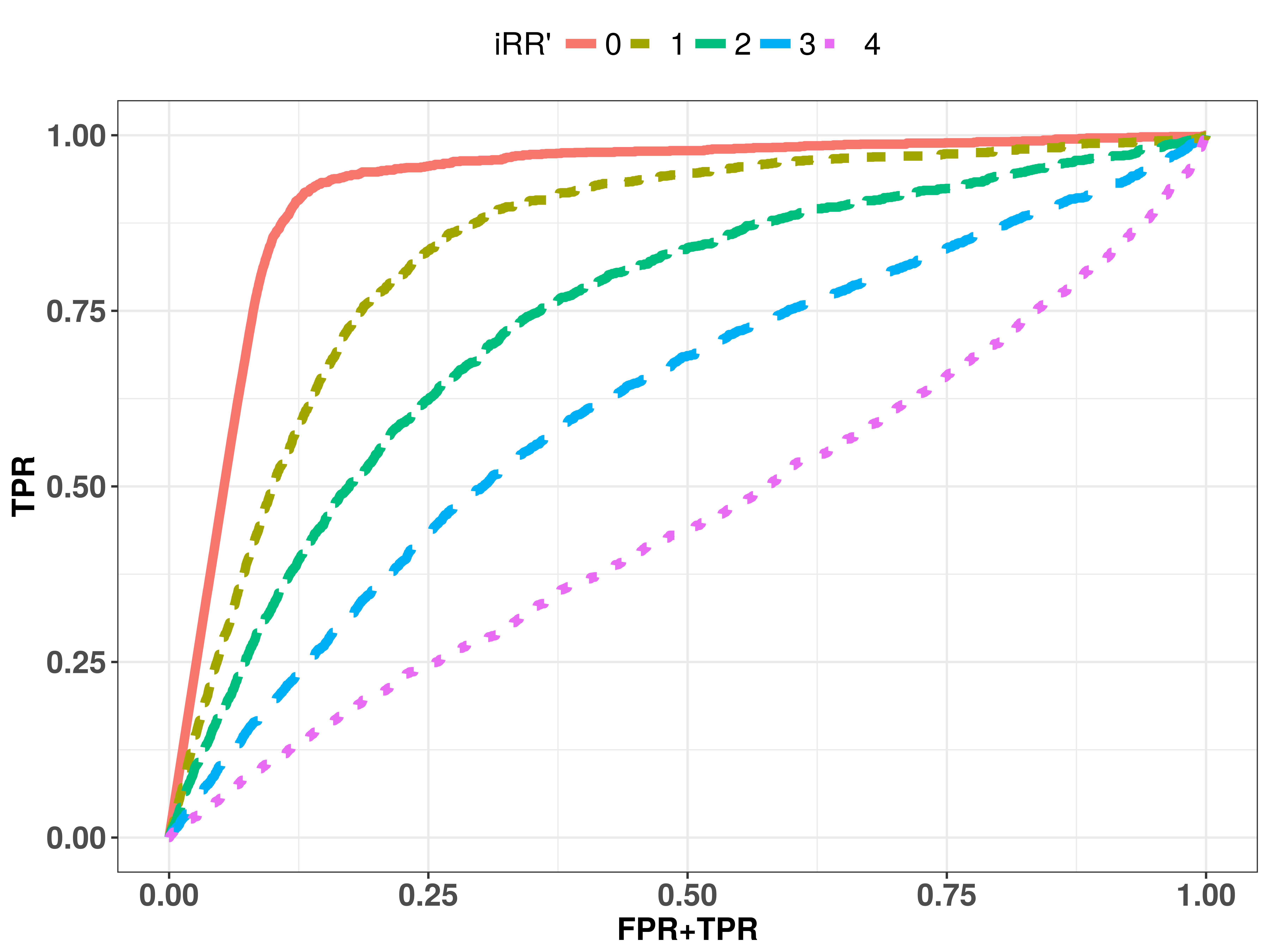
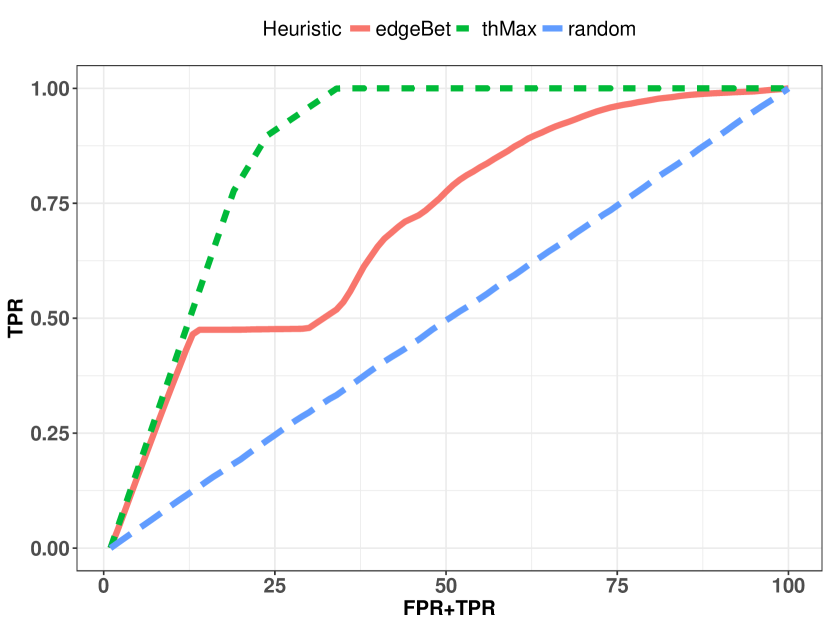
Figure 3: Feasibility of tagging biased edges: ROC curves for an edge-betweenness tagging algorithm. Model (left) and Youtube crawls (right).

A biased recommendation model

Our model considers two recommenders: one “official” $R$, and one used to issue “biased” recommendations, $R^{\prime}$. To model the fact that biased recommendations may not be completely unrelated to normal recommendations, we use a tuning parameter $i_{RR^{\prime}}$ presented hereafter. Let $R$ be a $k$NN recommendation system producing $k_{R}$ items per query ($\forall i\in V_{t},|R_{i}(u)|=k_{R}$), based on the $p_{i}\in\mathbb{R}^{d}$ feature vector: $\forall i,j\in V_{t}^{2},s^{i}_{R}(u,j)=||p_{i}p_{j}||_{2}$. Let $E_{t}$ be the set of produced edges.

In addition to its $p_{i}$ vector, each item $i\in V_{t}$ is associated with another $d^{\prime}$ dimensional feature vector $b_{i}\in\mathbb{R}^{d^{\prime}}$, representing “hidden” features (profitability, political support, …) leveraged to bias recommendation. Biased edge set $E_{t,R^{\prime}}$ is produced by a $k$NN recommender with $k_{B}$ output using $b_{i}$. The user-graph of recommendation is then $G_{t}(u)=(V_{t},E_{t}\cup E_{t,R^{\prime}})$ in which nodes have an out-degree of $k=k_{R}+k_{B}$.

Features are generated uniformly at random: $\forall i\in V_{t}:(p_{i}[c])_{1\leq c\leq d}\sim U(0,1)$ and $(b_{i}[c])_{1\leq c\leq d^{\prime}}\sim U(0,1)$. However, to vary the amount of bias, the dependency between $p_{i}$ and $b_{i}$ is as following: let $0\leq i_{RR^{\prime}}\leq min(d,d^{\prime})$. We set $\forall i\in V_{t},\forall 1\leq c\leq i_{RR^{\prime}},b_{i}[c]\leftarrow p_{i}[c]$. That is, if $d=d^{\prime}=i_{RR^{\prime}}$, both recommenders $R$ and $R^{\prime}$ will produce exactly the same results (and therefore equivalent user-graphs of recommendations). On the other hand, if $i_{RR^{\prime}}=0$, $p_{i}$ and $b_{i}$ are independent, and so are the results of $R$ and $R^{\prime}$.

3.2 Experiments

We use three Youtube crawls, such as the one presented as $\mathcal{C}$ (Section 1), from a returning user $u$, and from the same Lady Gaga video (with around one month delay between each of them). In the set of Youtube recommendations at each page, some (around $20\%$) are tagged with the flag “Recommended for you” (whereas other videos simply display their number of views). For the experiment, we consider those recommendations as part of the biased set we seek to tag (i.e., the ground truth). We parameter the model for comparable topology properties: $|V_{t}|=8753,k_{R}=17,k_{B}=2$. We set $d=d^{\prime}=5$.

First, we look at the small-world parallel with introduced bias under Proposition 1 on Figure 2, where we plot the path length distribution of respectively one $\hat{G}_{t}^{4}(u,i)$ observation (said biased) where $i$ is the Lady Gaga video, and one $\hat{G}_{t}^{4}(u,i)\setminus E_{t,R^{\prime}}$ (said unbiased), i.e., we respectively use the YouTube full crawl, and then remove the “Recommended for you” edges to obtain the unbiased graph.

We note a clear change in the graph properties when biased edges are present: they shortcut many paths, and then cause a more compact distribution of lengths, on both the model and the Youtube crawl. This exact effect of long edges is a well studied feature of small-world graphs [14].

Second, Proposition 2 is examined on Figure 3. For doing so, we run a symmetric edge-betweenness centrality [7] algorithm on $\hat{G}_{t}^{4}(u,i)$ graphs, for that metric is aimed at finding topologically important edges (typically linking clusters). We plot the ROC curves, representing the probability of biased edges actually ending-up in sorted top-result of the centrality metric (note that the the Youtube experiment, the plot is the average result over the three crawls). For the model, independent set of edges ($iRR$=0) indicates the awaited ease to differentiate them, while a bias based on few feature dependencies (e.g., $iRR^{\prime}$=1 or 2) also clearly allows for accurate edge tagging. For Youtube, the heuristic is also significantly above a random tagging baseline, close to the maximum possible (thMax) at the beginning of the experiment (i.e., top-ranked edges are indeed all biased). There is then a plateau regime (following top-ranked edges are mistagged), after which accurate tagging progresses smoothly. For both experiments, we conclude that tagging algorithms, to be proposed, have a clear room for providing accurate results: if one seeks the $4491$ biased edges of the dataset, the edge-betweenness algorithm on Youtube directly allows to identify close to $50\%$ of the biased set, at $x=12.5\%$.

4 Related Work

The usage of graph representations are common in the literature of recommender systems, for analyzing their input datasets, and adapt recommender algorithms accordingly. Notably, authors of [10] propose multiple graph representations of input of a recommender dataset (ratings, users, items): a bipartite graph of users and items, a “social network” of users having consumed the same items, and both the previous graphs with a so called recommender graph. Dataset is assumed to be the resulting of users activity in the system following recommendations. They show the approach useful for comparing recommender algorithms as a function of the pairs of users they are connecting a posteriori. Authors of [6] propose to build a graph of items, item categories and users (with edges being the number of times a user consumed an item), and perform random walks over that graph to find nodes similarities. The temporality of user preferences (long-term and short-term) are incorporated with approach in [15] to build an input (bipartite) graph that is then leveraged by a random walk-based method to issue recommendations (similar to personalized Pagerank). Our work differs in that we aim to analyze the output of recommenders, possibly at runtime. Our models and proposed analysis rely on a item-item graph representation.

There is a recent research focus on providing tools capable of assessing the behavior of remote algorithms. XRay [9] proposes a Bayesian approach for inferring which data of a user profile, given as an input, is associated to a personalized ad to that user. Authors in [8] propose a graph theoretic approach to gain understanding on which centrality metrics are in use by platforms that offer peer-ranking services. Work in [13] shows that machine learning models can be extracted by a user from the cloud platform were they reside. Regarding recommender systems, paper [12] exposes the users perspective on what they wait from recommendation; interestingly, transparency was already a concern in 2001. Yet, despite a recent rise of concerns, they are not yet well identified tools to start addressing the problem from an observer (user) standpoint.

5 Conclusion

There are two main conclusions to this study. First, graphs are an interesting - yet vastly unexplored - tool for analyzing recommender outputs. Graphs of recommendations may be leveraged by service operators to compute general metrics about the consequence of their recommendations to users, in the light of e.g., Pagerank applied to the graph of web-pages. User-graphs of recommendations, when observed by users themselves may also carry information: they clearly display the item locality a service provides users with; we illustrate this through the clustering of recommendations to a returning user and later make the parallel with the small-world phenomenon.

Second, we believe that the representation of user-graphs of recommendations are of important interest for the growing domain of algorithmic transparency: if a service aims at biasing some recommendations, the effects might be witnessed on graph topologies.

We believe these conclusions bring both analytical and algorithmic interest in the scope of the study of personalization transparency. Future work includes generalization to other recommender types (e.g., neural network based), and other applications of those graphs of recommendations.

References

- [1] S. Agarwal, D. Borthakur, and I. Stoica. Snapshots in the hadoop distributed file system. In UC Berkeley Technical Report UCB/EECS, 2011.
- [2] A. Blum, T.-H. H. Chan, and M. R. Rwebangira. A random-surfer web-graph model. In ANALCO, 2006.
- [3] A. Casteigts, P. Flocchini, W. Quattrociocchi, and N. Santoro. Time-varying graphs and dynamic networks. In H. Frey, X. Li, and S. Ruehrup, editors, ADHOC-NOW, 2011.
- [4] P. Covington, J. Adams, and E. Sargin. Deep neural networks for youtube recommendations. In RecSys, 2016.
- [5] J. Davidson, B. Liebald, J. Liu, P. Nandy, T. Van Vleet, U. Gargi, S. Gupta, Y. He, M. Lambert, B. Livingston, and D. Sampath. The youtube video recommendation system. In RecSys, 2010.
- [6] F. Fouss, A. Pirotte, J. m. Renders, and M. Saerens. Random-walk computation of similarities between nodes of a graph with application to collaborative recommendation. IEEE Transactions on Knowledge and Data Engineering, 19(3):355–369, March 2007.
- [7] M. Girvan and M. E. J. Newman. Community structure in social and biological networks. Proceedings of the National Academy of Sciences, 99(12):7821–7826, 2002.
- [8] E. Le Merrer and G. Trédan. Uncovering influence cookbooks : Reverse engineering the topological impact in peer ranking services. In CSCW, 2017.
- [9] M. Lécuyer, G. Ducoffe, F. Lan, A. Papancea, T. Petsios, R. Spahn, A. Chaintreau, and R. Geambasu. Xray: Enhancing the web’s transparency with differential correlation. In USENIX Security Symposium, 2014.
- [10] B. J. Mirza, B. J. Keller, and N. Ramakrishnan. Studying recommendation algorithms by graph analysis. Journal of Intelligent Information Systems, 20(2):131–160, 2003.
- [11] F. Ricci, L. Rokach, B. Shapira, and P. B. Kantor. Recommender Systems Handbook. 1st edition, 2010.
- [12] S. Sinha, K. S. Rashmi, and R. Sinha. Beyond algorithms: An hci perspective on recommender systems, 2001.
- [13] F. Tramèr, F. Zhang, A. Juels, M. K. Reiter, and T. Ristenpart. Stealing machine learning models via prediction apis. In USENIX Security Symposium, 2016.
- [14] D. J. Watts and S. H. Strogatz. Collective dynamics of’small-world’networks. Nature, 393(6684):409–10, 1998.
- [15] L. Xiang, Q. Yuan, S. Zhao, L. Chen, X. Zhang, Q. Yang, and J. Sun. Temporal recommendation on graphs via long- and short-term preference fusion. In KDD, 2010.