Parseval Networks: Improving Robustness to Adversarial Examples

Abstract

We introduce Parseval networks, a form of deep neural networks in which the Lipschitz constant of linear, convolutional and aggregation layers is constrained to be smaller than $1$. Parseval networks are empirically and theoretically motivated by an analysis of the robustness of the predictions made by deep neural networks when their input is subject to an adversarial perturbation. The most important feature of Parseval networks is to maintain weight matrices of linear and convolutional layers to be (approximately) Parseval tight frames, which are extensions of orthogonal matrices to non-square matrices. We describe how these constraints can be maintained efficiently during SGD. We show that Parseval networks match the state-of-the-art in terms of accuracy on CIFAR-10/100 and Street View House Numbers (SVHN), while being more robust than their vanilla counterpart against adversarial examples. Incidentally, Parseval networks also tend to train faster and make a better usage of the full capacity of the networks.

1 Introduction

Deep neural networks achieve near-human accuracy on many perception tasks (He et al., 2016; Amodei et al., 2015). However, they lack robustness to small alterations of the inputs at test time (Szegedy et al., 2014). Indeed when presented with a corrupted image that is barely distinguishable from a legitimate one by a human, they can predict incorrect labels, with high-confidence. An adversary can design such so-called adversarial examples, by adding a small perturbation to a legitimate input to maximize the likelihood of an incorrect class under constraints on the magnitude of the perturbation (Szegedy et al., 2014; Goodfellow et al., 2015; Moosavi-Dezfooli et al., 2015; Papernot et al., 2016a). In practice, for a significant portion of inputs, a single step in the direction of the gradient sign is sufficient to generate an adversarial example (Goodfellow et al., 2015) that is even transferable from one network to another one trained for the same problem but with a different architecture (Liu et al., 2016; Kurakin et al., 2016).

The existence of transferable adversarial examples has two undesirable corollaries. First, it creates a security threat for production systems by enabling black-box attacks (Papernot et al., 2016a). Second, it underlines the lack of robustness of neural networks and questions their ability to generalize in settings where the train and test distributions can be (slightly) different as is the case for the distributions of legitimate and adversarial examples.

Whereas the earliest works on adversarial examples already suggested that their existence was related to the magnitude of the hidden activations gradient with respect to their inputs (Szegedy et al., 2014), they also empirically assessed that standard regularization schemes such as weight decay or training with random noise do not solve the problem (Goodfellow et al., 2015; Fawzi et al., 2016). The current mainstream approach to improving the robustness of deep networks is adversarial training. It consists in generating adversarial examples on-line using the current network’s parameters (Goodfellow et al., 2015; Miyato et al., 2015; Moosavi-Dezfooli et al., 2015; Szegedy et al., 2014; Kurakin et al., 2016) and adding them to the training data. This data augmentation method can be interpreted as a robust optimization procedure (Shaham et al., 2015).

In this paper, we introduce Parseval networks, a layerwise regularization method for reducing the network’s sensitivity to small perturbations by carefully controlling its global Lipschitz constant. Since the network is a composition of functions represented by its layers, we achieve increased robustness by maintaining a small Lipschitz constant (e.g., 1) at every hidden layer; be it fully-connected, convolutional or residual. In particular, a critical quantity governing the local Lipschitz constant in both fully connected and convolutional layers is the spectral norm of the weight matrix. Our main idea is to control this norm by parameterizing the network with parseval tight frames (Kovačević & Chebira, 2008), a generalization of orthogonal matrices.

The idea that regularizing the spectral norm of each weight matrix could help in the context of robustness appeared as early as (Szegedy et al., 2014), but no experiment nor algorithm was proposed, and no clear conclusion was drawn on how to deal with convolutional layers. Previous work, such as double backpropagation (Drucker & Le Cun, 1992) has also explored jacobian normalization as a way to improve generalization. Our contribution is twofold. First, we provide a deeper analysis which applies to fully connected networks, convolutional networks, as well as Residual networks (He et al., 2016). Second, we propose a computationally efficient algorithm and validate its effectiveness on standard benchmark datasets. We report results on MNIST, CIFAR-10, CIFAR-100 and Street View House Numbers (SVHN), in which fully connected and wide residual networks were trained (Zagoruyko & Komodakis, 2016) with Parseval regularization. The accuracy of Parseval networks on legitimate test examples matches the state-of-the-art, while the results show notable improvements on adversarial examples. Besides, Parseval networks train significantly faster than their vanilla counterpart.

In the remainder of the paper, we first discuss the previous work on adversarial examples. Next, we give formal definitions of the adversarial examples and provide an analysis of the robustness of deep neural networks. Then, we introduce Parseval networks and its efficient training algorithm. Section 5 presents experimental results validating the model and providing several insights.

2 Related work

Early papers on adversarial examples attributed the vulnerability of deep networks to high local variations (Szegedy et al., 2014; Goodfellow et al., 2015). Some authors argued that this sensitivity of deep networks to small changes in their inputs is because neural networks only learn the discriminative information sufficient to obtain good accuracy rather than capturing the true concepts defining the classes (Fawzi et al., 2015; Nguyen et al., 2015).

Strategies to improve the robustness of deep networks include defensive distillation (Papernot et al., 2016b), as well as various regularization procedures such as contractive networks (Gu & Rigazio, 2015). However, the bulk of recent proposals relies on data augmentation (Goodfellow et al., 2015; Miyato et al., 2015; Moosavi-Dezfooli et al., 2015; Shaham et al., 2015; Szegedy et al., 2014; Kurakin et al., 2016). It uses adversarial examples generated online during training. As we shall see in the experimental section, regularization can be complemented with data augmentation; in particular, Parseval networks with data augmentation appear more robust than either data augmentation or Parseval networks considered in isolation.

3 Robustness in Neural Networks

We consider a multiclass prediction setting, where we have $Y$ classes in ${\cal Y}=\{1,...,Y\}$. A multiclass classifier is a function $\hat{g}:(x\in\mathbb{R}^{D},W\in{\cal W})\mapsto\operatorname*{argmax}_{{\bar{y}}\in{\cal Y}}g_{\bar{y}}(x,W)$, where $W$ are the parameters to be learnt, and $g_{\bar{y}}(x,W)$ is the score given to the (input, class) pair $(x,{\bar{y}})$ by a function $g:\mathbb{R}^{D}\times{\cal W}\rightarrow\mathbb{R}^{Y}$. We take $g$ to be a neural network, represented by a computation graph $G=({\cal N},{\cal E})$, which is a directed acyclic graph with a single root node, and each node $n\in{\cal N}$ takes values in $\mathbb{R}^{d_{out}^{(n)}}$ and is a function of its children in the graph, with learnable parameters $W^{(n)}$:

$$n:x\mapsto\phi^{(n)}\big{(}W^{(n)},\big{(}n^{\prime}(x)\big{)}_{n^{\prime}:(n,n^{\prime})\in{\cal E}}\big{)}\,.$$ (1)

The function $g$ we want to learn is the root of $G$. The training data $((x_{i},y_{i}))_{i=1}^{m}\in({{\cal X}}\times{\cal Y})^{m}$ is an i.i.d. sample of ${\cal D}$, and we assume ${\cal X}\subset\mathbb{R}^{D}$ is compact. A function $\ell:\mathbb{R}^{Y}\times{\cal Y}\rightarrow\mathbb{R}$ measures the loss of $g$ on an example $(x,y)$; in a single-label classification setting for instance, a common choice for $\ell$ is the log-loss:

$$\ell\big{(}g(x,W),y\big{)}=-g_{y}(x,W)+\log\big{(}\sum_{{\bar{y}}\in{\cal Y}}e^{g_{{\bar{y}}}(x,W)}\big{)}.\!\!$$ (2)

The arguments that we develop below depend only on the Lipschitz constant of the loss, with respect to the norm of interest. Formally, we assume that given a $p$-norm of interest $\|.\|_{p}$, there is a constant $\lambda_{p}$ such that

$$\forall z,z^{\prime}\in\mathbb{R}^{Y},\forall{\bar{y}}\in{\cal Y},|\ell(z,{\bar{y}})-\ell(z^{\prime},{\bar{y}})|\leq\lambda_{p}\|z-z^{\prime}\|_{p}\,.$$ (3)

For the log-loss of (2), we have $\lambda_{2}\leq\sqrt{2}$ and $\lambda_{\infty}\leq 2$. In the next subsection, we define adversarial examples and the generalization performance of the classifier. Then, we make the relationship between robustness to adversarial examples and the lipschitz constant of the networks.

3.1 Adversarial examples

Given an input (train or test) example $(x,y)$, an adversarial example is a perturbation of the input pattern $\tilde{x}=x+\delta_{x}$ where $\delta_{x}$ is small enough so that $\tilde{x}$ is nearly undistinguishable from $x$ (at least from the point of view of a human annotator), but has the network predict an incorrect label. Given the network parameters and structure $g(.,W)$ and a $p$-norm, the adversarial example is formally defined as

$$\tilde{x}=\operatorname*{argmax}_{\tilde{x}:\|\tilde{x}-x\|_{p}\leq\epsilon}\ell\big{(}g(\tilde{x},W),y\big{)}\,,$$ (4)

where $\epsilon$ represents the strength of the adversary. Since the optimization problem above is non-convex, Shaham et al. (2015) propose to take the first order taylor expansion of $x\mapsto\ell(g(x,W),y)$ to compute $\delta_{x}$ by solving

$$\tilde{x}=\operatorname*{argmax}_{\tilde{x}:\|\tilde{x}-x\|_{p}\leq\epsilon}\big{(}\nabla_{x}\ell(g(x,W),y)\big{)}^{T}(\tilde{x}-x)\,.$$ (5)

If $p=\infty$, then $\tilde{x}=x+\epsilon\text{sign}(\nabla_{x}\ell(g(x,W),y))$. This is the fast gradient sign method. For the case $p=2$, we obtain $\tilde{x}=x+\epsilon\nabla_{x}\ell(g(x,W),y)$. A more involved method is the iterative fast gradient sign method, in which several gradient steps of (5) are performed with a smaller stepsize to obtain a local minimum of (4).

3.2 Generalization with adversarial examples

In the context of adversarial examples, there are two different generalization errors of interest:

$$L(W) =\mathop{\mathbb{E}}\limits_{(x,y)\sim{\cal D}}\big{[}\ell(g(x,W),y)\big{]}\!\!\,,$$

$$L_{adv}(W,p,\epsilon) =\mathop{\mathbb{E}}\limits_{(x,y)\sim{\cal D}}\big{[}\max_{\tilde{x}:\|\tilde{x}-x\|_{p}\leq\epsilon}\ell(g(\tilde{x},W),y)\big{]}\!\!\,.$$

By definition, $L(W)\leq L_{adv}(W,p,\epsilon)$ for every $p$ and $\epsilon\!>\!0$. Reciprocally, denoting by $\lambda_{p}$ and $\Lambda_{p}$ the Lipschitz constant (with respect to $\|.\|_{p}$) of $\ell$ and $g$ respectively, we have:

$$\begin{split}&L_{adv}(W,p,\epsilon)\leq L(W)\\ &+\mathop{\mathbb{E}}\limits_{(x,y)\sim{\cal D}}\big{[}\max_{\tilde{x}:\|\tilde{x}-x\|_{p}\leq\epsilon}|\ell(g(\tilde{x},W),y)-\ell(g(x,W),y)|\big{]}\!\!\\ &\phantom{L_{adv}(W,p,\epsilon)}\leq L(W)+\lambda_{p}\Lambda_{p}\epsilon\,.\end{split}$$

This suggests that the sensitivity to adversarial examples can be controlled by the Lipschitz constant of the network. In the robustness framework of (Xu & Mannor, 2012), the Lipschitz constant also controls the difference between the average loss on the training set and the generalization performance. More precisely, let us denote by ${\cal C}_{p}({\cal X},\gamma)$ the covering number of ${\cal X}$ using $\gamma$-balls for $\|.\|_{p}$. Using $M=\sup_{x,W,y}\ell(g(x,W),y)$, Theorem 3 of (Xu & Mannor, 2012) implies that for every $\delta\in(0,1)$, with probability $1-\delta$ over the i.i.d. sample $((x_{i},y_{i})_{i=1}^{m}$, we have:

$$L(W)\leq \frac{1}{m}\sum_{i=1}^{m}\ell(g(x_{i},W),y_{i})$$

$$+\lambda_{p}\Lambda_{p}\gamma+M\sqrt{\frac{2Y{\cal C}_{p}({\cal X},\frac{\gamma}{2})\ln(2)-2\ln(\delta)}{m}}\,.$$

Since covering numbers of a $p$-norm ball in $\mathbb{R}^{D}$ increases exponentially with $\mathbb{R}^{D}$, the bound above suggests that it is critical to control the Lipschitz constant of $g$, for both good generalization and robustness to adversarial examples.

3.3 Lipschitz constant of neural networks

From the network structure we consider (1), for every node $n\in{\cal N}$, we have (see below for the definition of $\Lambda_{p}^{(n,n^{\prime})}$):

$$\|n(x)-n(\tilde{x})\|_{p}\leq\sum_{n^{\prime}:(n,n^{\prime})\in{\cal E}}\Lambda_{p}^{(n,n^{\prime})}\|n^{\prime}(x)-n^{\prime}(\tilde{x})\|_{p}\,,$$

for any $\Lambda_{p}^{(n,n^{\prime})}$ that is greater than the worst case variation of $n$ with respect to a change in its input $n^{\prime}(x)$. In particular we can take for $\Lambda_{p}^{(n,n^{\prime})}$ any value greater than the supremum over $x_{0}\in{\cal X}$ of the Lipschitz constant for $\|.\|_{p}$ of the function ($\mathbbm{1}_{n^{\prime\prime}=n^{\prime}}$ is $1$ if $n^{\prime\prime}=n^{\prime}$ and $0$ otherwise):

$$x\mapsto\phi^{(n)}\big{(}W^{(n)},\big{(}n^{\prime\prime}(x_{0}+\mathbbm{1}_{n^{\prime\prime}=n^{\prime}}(x-x_{0}))\big{)}_{n^{\prime\prime}:(n,n^{\prime\prime})\in{\cal E}}\big{)}\,.$$

The Lipschitz constant of $n$, denoted by $\Lambda_{p}^{(n)}$ satisfies:

$$\Lambda_{p}^{(n)}\leq\sum_{n^{\prime}:(n,n^{\prime})\in{\cal E}}\Lambda_{p}^{(n,n^{\prime})}\Lambda_{p}^{(n^{\prime})}$$ (6)

Thus, the Lipschitz constant of the network $g$ can grow exponentially with its depth. We now give the Lipschitz constants of standard layers as a function of their parameters:

Linear layers:

For layer $n(x)=W^{(n)}n^{\prime}(x)$ where $n^{\prime}$ is the unique child of $n$ in the graph, the Lipschitz constant for $\|.\|_{p}$ is, by definition, the matrix norm of $W^{(n)}$ induced by $\|.\|_{p}$, which is usually denoted $\|W^{(n)}\|_{p}$ and defined by

$$\|W^{(n)}\|_{p}=\sup_{z:\|z\|_{p}=1}\|W^{(n)}z\|_{p}\,.$$

Then $\Lambda_{2}^{(n)}=\|W^{(n)}\|_{2}\Lambda_{2}^{(n^{\prime})}$, where $\|W^{(n)}\|_{2}$, called the spectral norm of $W^{(n)}$, is the maximum singular value of $W^{(n)}$. We also have $\Lambda_{\infty}^{(n)}=\|W^{(n)}\|_{\infty}\Lambda_{\infty}^{(n^{\prime})}$, where $\|W^{(n)}\|_{\infty}=\max_{i}\sum_{j}|W^{(n)}_{ij}|$ is the maximum $1$-norm of the rows. $W^{(n)}$.

Convolutional layers:

To simplify notation, let us consider convolutions on 1D inputs without striding, and we take the width of the convolution to be $2k+1$ for $k\in\mathbb{N}$. To write convolutional layers in the same way as linear layers, we first define an unfolding operator $U$, which prepares the input $z$, denoted by $U(z)$. If the input has length $T$ with $d_{in}$ inputs channels, the unfolding operator maps $z$ For a convolution of the unfolding of $z$ considered as a $T\times(2k+1)d_{in}$ matrix, its $j$-th column is:

$$U_{j}(z)=[z_{j-k};...;z_{j+k}]\,,$$ (7)

where “;” is the concatenation along the vertical axis (each $z_{i}$ is seen as a column $d_{in}$-dimensional vector), and $z_{i}=0$ if $i$ is out of bounds ($0$-padding). A convolutional layer with $d_{out}$ output channels is then defined as

$$n(x)=W^{(n)}\ast n^{\prime}(x)=W^{(n)}U(n^{\prime}(x))\,,$$ (8)

where $W^{(n)}$ is a $d_{out}\times(2k+1)d_{in}$ matrix. We thus have $\Lambda_{2}^{(n)}\leq\|W\|_{2}\|U(n^{\prime}(x))\|_{2}$. Since $U$ is a linear operator that essentially repeats its input $(2k+1)$ times, we have $\|U(n^{\prime}(x))-U(n^{\prime}(\tilde{x}))\|_{2}^{2}\leq(2k+1)\|n^{\prime}(x)-n^{\prime}(\tilde{x})\|_{2}^{2}$, so that $\Lambda_{2}^{(n)}\leq\sqrt{2k+1}\|W\|_{2}\Lambda_{2}^{(n^{\prime})}$. Also, $\|U(n^{\prime}(x))-U(n^{\prime}(\tilde{x}))\|_{\infty}=\|n^{\prime}(x)-n^{\prime}(\tilde{x})\|_{\infty}$, and so for a convolutional layer, $\Lambda_{\infty}^{(n)}\leq\|W^{(n)}\|_{\infty}\Lambda_{\infty}^{(n^{\prime})}$.

Aggregation layers/transfer functions:

Layers that perform the sum of their inputs, as in Residual Netowrks (He et al., 2016), fall in the case where the values $\Lambda_{p}^{(n,n^{\prime})}$ in (6) come into play. For a node $n$ that sums its inputs, we have $\Lambda_{p}^{(n,n^{\prime})}=1$, and thus $\Lambda_{p}^{(n)}\leq\sum_{n^{\prime}:(n,n^{\prime})\in{\cal E}}\Lambda_{p}^{(n^{\prime})}$ . If $n$ is a tranfer function layer (e.g., an element-wise application of ReLU) we can check that $\Lambda_{p}^{(n)}\leq\Lambda_{p}^{(n^{\prime})}$, where $n^{\prime}$ is the input node, as soon as the Lipschitz constant of the transfer function (as a function $\mathbb{R}\rightarrow\mathbb{R}$) is $\leq 1$.

4 Parseval networks

Parseval regularization, which we introduce in this section, is a regularization scheme to make deep neural networks robust, by constraining the Lipschitz constant (6) of each hidden layer to be smaller than one, assuming the Lipschitz constant of children nodes is smaller than one. That way, we avoid the exponential growth of the Lipschitz constant, and a usual regularization scheme (i.e., weight decay) at the last layer then controls the overall Lipschitz constant of the network. To enforce these constraints in practice, Parseval networks use two ideas: maintaining orthonormal rows in linear/convolutional layers, and performing convex combinations in aggregation layers. Below, we first explain the rationale of these constraints and then describe our approach to efficiently enforce the constraints during training.

4.1 Parseval Regularization

Orthonormality of weight matrices:

For linear layers, we need to maintain the spectral norm of the weight matrix at $1$. Computing the largest singular value of weight matrices is not practical in an SGD setting unless the rows of the matrix are kept orthogonal. For a weight matrix $W\in\mathbb{R}^{d_{out}\times d_{in}}$ with $d_{out}\leq d_{in}$, Parseval regularization maintains $W^{T}W\approx I_{d_{out}\times d_{out}}$, where $I$ refers to the identity matrix. $W$ is then approximately a Parseval tight frame (Kovačević & Chebira, 2008), hence the name of Parseval networks. For convolutional layers, the matrix $W\in\mathbb{R}^{d_{out}\times(2k+1)d_{in}}$ is constrained to be a Parseval tight frame (with the notations of the previous section), and the output is rescaled by a factor $(2k+1)^{-1/2}$. This maintains all singular values of $W$ to $(2k+1)^{-1/2}$, so that $\Lambda_{2}^{(n)}\leq\Lambda_{2}^{(n^{\prime})}$ where $n^{\prime}$ is the input node. More generally, keeping the rows of weight matrices orthogonal makes it possible to control both the spectral norm and the $\|.\|_{\infty}$ of a weight matrix through the norm of its individual rows. Robustness for $\|.\|_{\infty}$ is achieved by rescaling the rows so that their $1$-norm is smaller than $1$. For now, we only experimented with constraints on the $2$-norm of the rows, so we aim for robustness in the sense of $\|.\|_{2}$.

Remark 1 (Orthogonality is required).

Without orthogonality, constraints on the $2$-norm of the rows of weight matrices are not sufficient to control the spectral norm. Parseval networks are thus fundamentally different from weight normalization (Salimans & Kingma, 2016).

Aggregation Layers:

In parseval networks, aggregation layers do not make the sum of their inputs, but rather take a convex combination of them:

$$n(x)=\sum_{n^{\prime}:(n,n^{\prime})\in{\cal E}}\alpha^{(n,n^{\prime})}n^{\prime}(x)$$ (9)

with $\sum_{n^{\prime}:(n,n^{\prime})\in{\cal E}}\alpha^{(n,n^{\prime})}=1$ and $\alpha^{(n,n^{\prime})}\geq 0$. The parameters $\alpha^{(n,n^{\prime})}$ are learnt, but using (6), these constraint guarantee that $\Lambda_{p}^{(n)}\leq 1$ as soon as the children satisfy the inequality for the same $p$-norm.

4.2 Parseval Training

Orthonormality constraints:

The first significant difference between Parseval networks and its vanilla counterpart is the orthogonality constraint on the weight matrices. This requirement calls for an optimization algorithm on the manifold of orthogonal matrices, namely the Stiefel manifold. Optimization on matrix manifolds is a well-studied topic (see (Absil et al., 2009) for a comprehensive survey). The simplest first-order geometry approaches consist in optimizing the unconstrained function of interest by moving in the direction of steepest descent (given by the gradient of the function) while at the same time staying on the manifold. To guarantee that we remain in the manifold after every parameter update, we need to define a retraction operator. There exist several pullback operators for embedded submanifolds such as the Stiefel manifold based for example on Cayley transforms (Absil et al., 2009). However, when learning the parameters of neural networks, these methods are computationally prohibitive. To overcome this difficulty, we use an approximate operator derived from the following layer-wise regularizer of weight matrices to ensure their parseval tightness (Kovačević & Chebira, 2008):

$$R_{\beta}(W_{k})=\frac{\beta}{2}\|W_{k}^{\top}W_{k}-I\|_{2}^{2}.$$ (10)

$\Theta=\{W_{k},\boldsymbol{\alpha}_{k}\}_{k=1}^{K}$, $e\leftarrow 0$
while  $e\leq E$  do

       Sample a minibatch $\{(x_{i},y_{i})\}_{i=1}^{B}$.
for $k\in\{1,\dots,K\}$ do

             Compute the gradient: $G_{W_{k}}\leftarrow\nabla_{W_{k}}\ell(\Theta,\{(x_{i},y_{i})\})$, $G_{\boldsymbol{\alpha}_{k}}\leftarrow\nabla_{\boldsymbol{\alpha}_{k}}\ell(\Theta,\{(x_{i},y_{i})\})$.
Update the parameters:
$W_{k}\leftarrow W_{k}-\epsilon\cdot G_{W_{k}}$
$\boldsymbol{\alpha}_{k}\leftarrow\boldsymbol{\alpha}_{k}-\epsilon\cdot G_{\boldsymbol{\alpha}_{k}}$.
if hidden layer then

                   Sample a subset $S$ of rows of $W_{k}$.
Projection:
$W_{S}\leftarrow(1+\beta)W_{S}-\beta W_{S}W_{S}^{\top}W_{S}$.
$\boldsymbol{\alpha}_{k}\leftarrow\operatorname*{argmin}_{\boldsymbol{\gamma}\in\Delta^{K-1}}\|\boldsymbol{\alpha}_{K}-\boldsymbol{\gamma}\|_{2}^{2}$

            

      $e\leftarrow e+1$.

Algorithm 1 Parseval Training

Optimizing $R_{\beta}(W_{k})$ to convergence after every gradient descent step (w.r.t the main objective) guarantees us to stay on the desired manifold but this is an expensive procedure. Moreover, it may result in parameters that are far from the ones obtained after the main gradient update. We use two approximations to make the algorithm more efficient: First, we only do one step of descent on the function $R_{\alpha}(W_{k})$. The gradient of this regularization term is $\nabla_{W_{k}}R_{\beta}(W_{k})=\beta(W_{k}W_{k}^{\top}-I)W_{k}$. Consequently, after every main update we perform the following secondary update:

$$W_{k}\leftarrow(1+\beta)W_{k}-\beta W_{k}W_{k}^{\top}W_{k}.$$ (11)

Optionally, instead of updating the whole matrix, one can randomly select a subset $S$ of rows and perform the update from Eq. (11) on the submatrix composed of rows indexed by $S$. This sampling based approach reduces the overall complexity to $\mathcal{O}(|S|^{2}d)$. Provided the rows are carefully sampled, the procedure is an accurate Monte Carlo approximation of the regularizer loss function (Drineas et al., 2006). The optimal sampling probabilities, also called statistical leverages are approximately equal if we start from an orthogonal matrix and (approximately) stay on the manifold throughout the optimization since they are proportional to the eigenvalues of $W$ (Mahoney et al., 2011). Therefore, we can sample a subset of columns uniformly at random when applying this projection step.

While the full update does not result in an increased overhead for convolutional layers, the picture can be very different for large fully connected layers making the sampling approach computationally more appealing for such layers. We show in the experiments that the weight matrices resulting from this procedure are (quasi)-orthogonal. Also, note that quasi-orthogonalization procedures similar to the one described here have been successfully used previously in the context of learning overcomplete representations with independent component analysis (Hyvärinen & Oja, 2000).

Convexity constraints in aggregation layers:

In Parseval networks, aggregation layers output a convex combination of their inputs instead of e.g., their sum as in Residual networks (He et al., 2016). For an aggregation node $n$ of the network, let us denote by $\boldsymbol{\alpha}=(\alpha^{(n,n^{\prime})})_{n^{\prime}:(n,n^{\prime})\in{\cal E}}$ the $K$-size vector of coefficients used for the convex combination output by the layer. To ensure that the Lipschitz constant at the node $n$ is such that $\Lambda_{p}^{(n)}\leq 1$, the constraints of 9 call for a euclidean projection of $\boldsymbol{\alpha}$ onto the positive simplex after a gradient update:

$$\boldsymbol{\alpha}^{*}=\operatorname*{argmin}_{\boldsymbol{\gamma}\in\Delta^{K-1}}\|\boldsymbol{\alpha}-\boldsymbol{\gamma}\|_{2}^{2}\,,$$ (12)

where $\Delta^{K-1}=\{\boldsymbol{\gamma}\in\mathbb{R}^{K}|\boldsymbol{1}^{\top}\boldsymbol{\gamma}=1,\boldsymbol{\gamma}\geq 0\}$. This is a well studied problem (Michelot, 1986; Pardalos & Kovoor, 1990; Duchi et al., 2008; Condat, 2016). Its solution is of the form: $\alpha^{*}_{i}=\max(0,\alpha_{i}-\tau(\boldsymbol{\alpha}))$, with $\tau:\mathbb{R}^{K}\rightarrow\mathbb{R}$ the unique function satisfying $\sum_{i}(x_{i}-\tau(\boldsymbol{\alpha}))=1$ for every $\boldsymbol{x}\in\mathbb{R}^{K}$. Therefore, the solution essentially boils down to a soft thresholding operation. If we denote $\alpha_{1}\geq\alpha_{2}\geq\dots\alpha_{K}$ the sorted coefficients and $k(\boldsymbol{\alpha})=\max\{k\in(1,\dots,K)|1+k\alpha_{k}>\sum_{j\leq k}\alpha_{j}\}$, the optimal thresholding is given by (Duchi et al., 2008):

$$\tau(\boldsymbol{\alpha})=\frac{(\sum_{j\leq k(\boldsymbol{\alpha})}\alpha_{j})-1}{k(\boldsymbol{\alpha})}$$ (13)

Consequently, the complexity of the projection is $O(K\log(K))$ since it is only dominated by the sorting of the coefficients and is typically cheap because aggregation nodes will only have few children in practice (e.g. 2). If the number of children is large, there exist efficient linear time algorithms for finding the optimal thresholding $\tau(\boldsymbol{\alpha})$ (Michelot, 1986; Pardalos & Kovoor, 1990; Condat, 2016). In this work, we use the method detailed above (Duchi et al., 2008) to perform the projection of the coefficient $\boldsymbol{\alpha}$ after every gradient update step.

5 Experimental evaluation

We evaluate the effectiveness of Parseval networks on well-established image classification benchmark datasets namely MNIST, CIFAR-10, CIFAR-100 (Krizhevsky, 2009) and Street View House Numbers (SVHN) (Netzer et al., ). We train both fully connected networks and wide residual networks. The details of the datasets, the models, and the training routines are summarized below.

Figure 1: Sample images from the CIFAR-10 dataset, with corresponding adversarial examples. We show the original image and adversarial versions for SNR values of 24.7, 12.1 and 7.8.

5.1 Datasets

CIFAR. Each of the CIFAR datasets is composed of 60K natural scene color images of size $32\times 32$ split between 50K training images and 10K test images. CIFAR-10 and CIFAR-100 have respectively 10 and 100 classes. For these two datasets, we adopt the following standard preprocessing and data augmentation scheme (Lin et al., 2013; He et al., 2016; Huang et al., 2016a; Zagoruyko & Komodakis, 2016): Each training image is first zero-padded with 4 pixels on each side. The resulting image is randomly cropped to produce a new $32\times 32$ image which is subsequently horizontally flipped with probability $0.5$. We also normalize every image with the mean and standard deviation of its channels. Following the same practice as (Huang et al., 2016a), we initially use 5K images from the training as a validation set. Next, we train de novo the best model on the full set of 50K images and report the results on the test set. SVHN The Street View House Number dataset is a set of $32\times 32$ color digit images officially split into 73257 training images and 26032 test images. Following common practice (Zagoruyko & Komodakis, 2016; He et al., 2016; Huang et al., 2016a, b), we randomly sample 10000 images from the available extra set of about $600K$ images as a validation set and combine the rest of the pictures with the official training set for a total number of 594388 training images. We divide the pixel values by 255 as a preprocessing step and report the test set performance of the best performing model on the validation set.

5.2 Models and Implementation details

5.2.1 ConvNets

Models. For the CIFAR and SVHN datasets, we trained wide residual networks (Zagoruyko & Komodakis, 2016) as they perform on par with standard resnets (He et al., 2016) while being faster to train thanks to a reduced depth. We used wide resnets of depth 28 and width 10 for both CIFAR-10 and CIFAR-100. For SVHN we used wide resnet of depth 16 and width 4. For each architecture, we compare Parseval networks with the vanilla model trained with standard regularization both in the adversarial and the non-adversarial training settings.

Training. We train the networks with stochastic gradient descent using a momentum of 0.9. On CIFAR datasets, the initial learning rate is set to $0.1$ and scaled by a factor of $0.2$ after epochs 60, 120 and 160, for a total number of 200 epochs. We used mini-batches of size 128. For SVHN, we trained the models with mini-batches of size 128 for 160 epochs starting with a learning rate of 0.01 and decreasing it by a factor of $0.1$ at epochs 80 and 120. For all the vanilla models, we applied by default weight decay regularization (with parameter $\lambda=0.0005$) together with batch normalization and dropout since this combination resulted in better accuracy and increased robustness in preliminary experiments. The dropout rate use is 0.3 for CIFAR and 0.4 for SVHN. For Parseval regularized models, we choose the value of the retraction parameter to be $\beta=0.0003$ for CIFAR datasets and $\beta=0.0001$ for SVHN based on the performance on the validation set. In all cases, We also adversarially trained each of the models on CIFAR-10 and CIFAR-100 following the guidelines in (Goodfellow et al., 2015; Shaham et al., 2015; Kurakin et al., 2016). In particular, we replace $50\%$ of the examples of every minibatch by their adversarially perturbed version generated using the one-step method to avoid label leaking (Kurakin et al., 2016). For each mini-batch, the magnitude of the adversarial perturbation is obtained by sampling from a truncated Gaussian centered at $0$ with standard deviation 2.

5.2.2 Fully Connected

Model. We also train feedforward networks composed of 4 fully connected hidden layers of size 2048 and a classification layer. The input to these networks are images unrolled into a $C\times 1024$ dimensional vector where $C$ is the number of channels. We used these models on MNIST and CIFAR-10 mainly to demonstrate that the proposed approach is also useful on non-convolutional networks. We compare a Parseval networks to vanilla models with and without weight decay regularization. For adversarially trained models, we follow the guidelines previously described for the convolutional networks.

Training. We train the models with SGD and divide the learning rate by two every 10 epochs. We use mini-batches of size 100 and train the model for 50 epochs. We chose the hyperparameters on the validation set and re-train the model on the union of the training and validation sets. The hyperparameters are $\beta$, the size of the row subset $S$, the learning rate and its decrease rate. Using a subset $S$ of $30\%$ of all the rows of each of weight matrix for the retraction step worked well in practice.

5.3 Results

5.3.1 (Quasi)-orthogonality.

We first validate that Parseval training (Algorithm 1) indeed yields (near)-orthonormal weight matrices. To do so, we analyze the spectrum of the weight matrices of the different models by plotting the histograms of their singular values, and compare these histograms for Parseval networks to networks trained using standard SGD with and without weight decay (SGD-wd and SGD).

Figure 2: Histograms of the singular values of the weight matrices at layers 1 and 4 of our network in CIFAR-10.

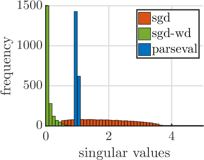
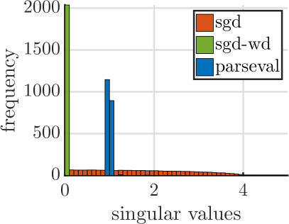
The histograms representing the distribution of singular values at layers 1 and 4 for the fully connected network (using $S=30\%$) trained on the dataset CIFAR-10 are shown in Fig. 2 (the figures for convolutional networks are similar). The singular values obtained with our method are tightly concentrated around 1. This experiment confirms that the weight matrices produced by the proposed optimization procedure are (almost) orthonormal. The distribution of the singular values of the weight matrices obtained with SGD has a lot more variance, with nearly as many small values as large ones. Adding weight decay to standard SGD leads to a sparse spectrum for the weight matrices, especially in the higher layers of the network suggesting a low-rank structure. This observation has motivated recent work on compressing deep neural networks (Denton et al., 2014).

5.3.2 Robustness to adversarial noise.

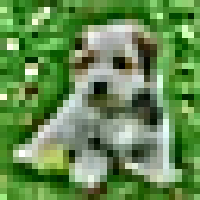
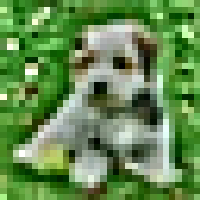
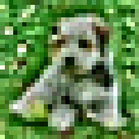
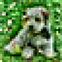
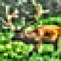
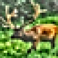
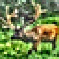
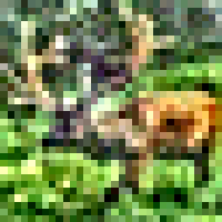
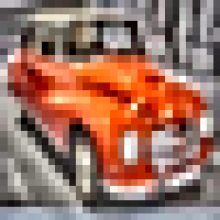
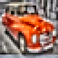
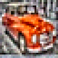
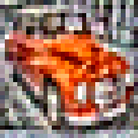
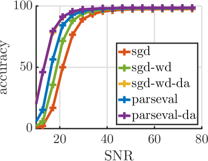
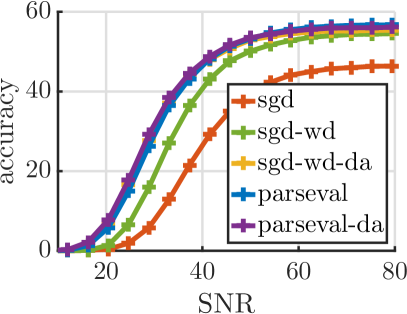
We evaluate the robustness of the models to adversarial noise by generating adversarial examples from the test set, for various magnitudes of the noise vector. Following common practice (Kurakin et al., 2016), we use the fast gradient sign method to generate the adversarial examples (using $\|.\|_{\infty}$, see Section 3.1). Since these adversarial examples transfer from one network to the other, the fast gradient sign method allows to benchmark the network for reasonable settings where the opponent does not know the network. We report the accuracy of each model as a function of the magnitude of the noise. To make the results easier to interpret, we compute the corresponding Signal to Noise Ratio (SNR). For an input $x$ and perturbation $\delta_{x}$, the SNR is defined as $\text{SNR}(x,\delta_{x})=20\log_{10}\frac{\|x\|_{2}}{\|\delta_{x}\|_{2}}$. We show some adversarial examples in Fig. 1.

Figure 3: Performance of the models for various magnitudes of adversarial noise on MNIST (left) and CIFAR-10 (right).

Table 1: Classification accuracy of the models on CIFAR-10 and CIFAR-100 with the (combination of) various regularization scheme. $\epsilon$ represents here the value of the signal to noise ratio (SNR). At $\epsilon=30$, an adversarially perturbed image is perceptible by a human. For each dataset, the top 3 rows report results for non-adversarial training and the bottom 3 rows report results for adversarial training.

	Model	Clean	$\epsilon\approx 50$	$\epsilon\approx 45$	$\epsilon\approx 40$	$\epsilon\approx 33$
CIFAR-10	Vanilla	95.63	90.16	85.97	76.62	67.21
	Parseval(OC)	95.82	91.85	88.56	78.79	61.38
	Parseval	96.28	93.03	90.40	81.76	69.10
	Vanilla	95.49	91.17	88.90	86.75	84.87
	Parseval(OC)	95.59	92.31	90.00	87.02	85.23
	Parseval	96.08	92.51	90.05	86.89	84.53
CIFAR-100	Vanilla	79.70	65.76	57.27	44.62	34.49
	Parseval(OC)	81.07	70.33	63.78	49.97	32.99
	Parseval	80.72	72.43	66.41	55.41	41.19
	Vanilla	79.23	67.06	62.53	56.71	51.78
	Parseval(OC)	80.34	69.27	62.93	53.21	52.60
	Parseval	80.19	73.41	67.16	58.86	39.56
SVHN	Vanilla	98.38	97.04	95.18	92.71	88.11
	Parseval(OC)	97.91	97.55	96.35	93.73	89.09
	Parseval	98.13	97.86	96.19	93.55	88.47

Fully Connected Nets.

Figure 3 depicts a comparison of Parseval and vanilla networks with and without adversarial training at various noise levels. On both MNIST and CIFAR-10, Parseval networks consistently outperforms weight decay regularization. In addition, it is as robust as adversarial training (SGD-wd-da) on CIFAR-10. Combining Parseval Networks and adversarial training results in the most robust method on MNIST.

ResNets.

Table 1 summarizes the results of our experiments with wide residual Parseval and vanilla networks on CIFAR-10, CIFAR-100 and SVHN. In the table, we denote Parseval(OC) the Parseval network with orthogonality constraint and without using a convex combination in aggregation layers. Parseval indicates the configuration where both of the orthogonality and convexity constraints are used. We first observe that Parseval networks outperform vanilla ones on all datasets on the clean examples and match the state of the art performances on CIFAR-10 $(96.28\%)$ and SVHN $(98.44\%)$. On CIFAR-100, when we use Parseval wide Resnet of depth 40 instead of 28, we achieve an accuracy of $81.76\%$. In comparison, the best performance achieved by a vanilla wide resnet (Zagoruyko & Komodakis, 2016) and a pre-activation resnet (He et al., 2016) are respectively $81.12\%$ and $77.29\%$. Therefore, our proposal is a useful regularizer for legitimate examples. Also note that in most cases, Parseval networks combining both the orthogonality constraint and the convexity constraint is superior to use the orthogonality constraint solely.

The results presented in the table validate our most important claim: Parseval networks significantly improve the robustness of vanilla models to adversarial examples. When no adversarial training is used, the gap in accuracy between the two methods is significant (particularly in the high noise scenario). For an SNR value of $40$, the best Parseval network achieves $55.41\%$ accuracy while the best vanilla model is at $44.62\%$. When the models are adversarially trained, Parseval networks remain superior to vanilla models in most cases. Interestingly, adversarial training only slightly improves the robustness of Parseval networks in low noise setting (e.g. SNR values of 45-50) and sometimes even deteriorates it (e.g. on CIFAR-10). In contrast, combining adversarial training and Parseval networks is an effective approach in the high noise setting. This result suggests that thanks to the particular form of regularizer (controlling the Lipschitz constant of the network), Parseval networks achieves robustness to adversarial examples located in the immediate vicinity of each data point. Therefore, adversarial training only helps for adversarial examples found further away from the legitimate patterns. This observation holds consistently across the datasets considered in this study.

5.3.3 Better use of capacity

Table 2: Number of dimensions (in $\%$ of the total dimension) necessary to capture 99% of the covariance of the activations.

		SGD-wd			SGD-wd-da			Parseval
		all	class		all	class		all	class
Layer 1		72.6	34.7		73.6	34.7		89.0	38.4
Layer 2		1.5	1.3		1.5	1.3		82.6	38.2
Layer 3		0.5	0.5		0.4	0.4		81.9	30.6
Layer 4		0.5	0.4		0.4	0.4		56.0	19.3

Given the distribution of singular values observed in Figure 2, we want to analyze the intrinsic dimensionality of the representation learned by the different networks at every layer. To that end, we use the local covariance dimension (Dasgupta & Freund, 2008) which can be measured from the covariance matrix of the data. For each layer $k$ of the fully connected network, we compute the activation’s empirical covariance matrix $\frac{1}{n}\sum_{i=1}^{n}\phi_{k}(x)\phi_{k}(x)^{\top}$ and obtain its sorted eigenvalues $\sigma_{1}\geq\dots\geq\sigma_{d}$. For each method and each layer, we select the smallest integer $p$ such that $\sum_{i=1}^{p}\sigma_{i}\geq 0.99\sum_{i=1}^{d}\sigma_{i}$. This gives us the number of dimensions that we need to explain $99\%$ of the covariance. We can also compute the same quantity for the examples of each class, by only considering in the empirical estimation of the covariance of the examples $x_{i}$ such that $y_{i}=c$. We report these numbers both on all examples and the per-class average on CIFAR-10 in Table 2.

Table 2 shows that the local covariance dimension of all the data is consistently higher for Parseval networks than all the other approaches at any layer of the network. SGD-wd-da contracts all the data in very low dimensional spaces at the upper levels of the network by using only $0.4\%$ of the total dimension (layer 3 and 4) while Parseval networks use about $81\%$ and $56\%$ at of the whole dimension respectively in the same layers. This is intriguing given that SGD-wd-da also increases the robustness of the network, apparently not in the same way as Parseval networks. For the average local covariance dimension of the classes, SGD-wd-da contracts each class into the same dimensionality as it contracts all the data at the upper layers of the network. For Parseval, the data of each class is contracted in about $30\%$ and $19\%$ of the overall dimension. These results suggest that Parseval contracts the data of each class in a lower dimensional manifold (compared to the intrinsic dimensionality of the whole data) hence making classification easier.

5.3.4 faster convergence

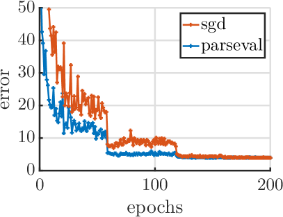
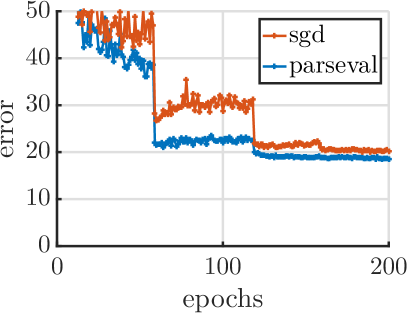
Parseval networks converge significantly faster than vanilla networks trained with batch normalization and dropout as depicted by figure 4. Thanks to the orthogonalization step following each gradient update, the weight matrices are well conditioned at each step during the optimization. We hypothesize this is the main explanation of this phenomenon. For convolutional networks (resnets), the faster convergence is not obtained at the expense of larger wall-time since the cost of the projection step is negligible compared to the total cost of the forward pass on modern GPU architecture thanks to the small size of the filters.

Figure 4: Learning curves of Parseval wide resnets and Vanilla wide resnets on CIFAR-10 (right) and CIFAR-100 (left). Parseval networks converge faster than their vanilla counterpart.

6 Conclusion

We introduced Parseval networks, a new approach for learning neural networks that are intrinsically robust to adversarial noise. We proposed an algorithm that allows us to optimize the model efficiently. Empirical results on three classification datasets with fully connected and wide residual networks illustrate the performance of our approach. As a byproduct of the regularization we propose, the model trains faster and makes a better use of its capacity. Further investigation of this phenomenon is left to future work.

References

- Absil et al. (2009) Absil, P-A, Mahony, Robert, and Sepulchre, Rodolphe. Optimization algorithms on matrix manifolds. Princeton University Press, 2009.
- Amodei et al. (2015) Amodei, Dario, Anubhai, Rishita, Battenberg, Eric, Case, Carl, Casper, Jared, Catanzaro, Bryan, Chen, Jingdong, Chrzanowski, Mike, Coates, Adam, Diamos, Greg, et al. Deep speech 2: End-to-end speech recognition in english and mandarin. arXiv preprint arXiv:1512.02595, 2015.
- Condat (2016) Condat, Laurent. Fast projection onto the simplex and the pmb l _ mathbf 1 ball. Mathematical Programming, 158(1-2):575–585, 2016.
- Dasgupta & Freund (2008) Dasgupta, Sanjoy and Freund, Yoav. Random projection trees and low dimensional manifolds. In Proceedings of the fortieth annual ACM symposium on Theory of computing, pp. 537–546. ACM, 2008.
- Denton et al. (2014) Denton, Emily L, Zaremba, Wojciech, Bruna, Joan, LeCun, Yann, and Fergus, Rob. Exploiting linear structure within convolutional networks for efficient evaluation. In Adv. NIPS, 2014.
- Drineas et al. (2006) Drineas, Petros, Kannan, Ravi, and Mahoney, Michael W. Fast monte carlo algorithms for matrices i: Approximating matrix multiplication. SIAM Journal on Computing, 36(1):132–157, 2006.
- Drucker & Le Cun (1992) Drucker, Harris and Le Cun, Yann. Improving generalization performance using double backpropagation. IEEE Transactions on Neural Networks, 3(6):991–997, 1992.
- Duchi et al. (2008) Duchi, John, Shalev-Shwartz, Shai, Singer, Yoram, and Chandra, Tushar. Efficient projections onto the l 1-ball for learning in high dimensions. In Proceedings of the 25th international conference on Machine learning, pp. 272–279. ACM, 2008.
- Fawzi et al. (2015) Fawzi, Alhussein, Fawzi, Omar, and Frossard, Pascal. Analysis of classifiers’ robustness to adversarial perturbations. arXiv preprint arXiv:1502.02590, 2015.
- Fawzi et al. (2016) Fawzi, Alhussein, Moosavi-Dezfooli, Seyed-Mohsen, and Frossard, Pascal. Robustness of classifiers: from adversarial to random noise. In Advances in Neural Information Processing Systems, pp. 1624–1632, 2016.
- Goodfellow et al. (2015) Goodfellow, Ian J, Shlens, Jonathon, and Szegedy, Christian. Explaining and harnessing adversarial examples. In Proc. ICLR, 2015.
- Gu & Rigazio (2015) Gu, Shixiang and Rigazio, Luca. Towards deep neural network architectures robust to adversarial examples. In ICLR workshop, 2015.
- He et al. (2016) He, Kaiming, Zhang, Xiangyu, Ren, Shaoqing, and Sun, Jian. Deep residual learning for image recognition. In Proceedings of the IEEE Conference on Computer Vision and Pattern Recognition, pp. 770–778, 2016.
- Huang et al. (2016a) Huang, Gao, Liu, Zhuang, Weinberger, Kilian Q, and van der Maaten, Laurens. Densely connected convolutional networks. arXiv preprint arXiv:1608.06993, 2016a.
- Huang et al. (2016b) Huang, Gao, Sun, Yu, Liu, Zhuang, Sedra, Daniel, and Weinberger, Kilian Q. Deep networks with stochastic depth. In European Conference on Computer Vision, pp. 646–661. Springer, 2016b.
- Hyvärinen & Oja (2000) Hyvärinen, Aapo and Oja, Erkki. Independent component analysis: algorithms and applications. Neural networks, 2000.
- Kovačević & Chebira (2008) Kovačević, Jelena and Chebira, Amina. An introduction to frames. Foundations and Trends in Signal Processing, 2008.
- Krizhevsky (2009) Krizhevsky, Alex. Learning multiple layers of features from tiny images, 2009.
- Kurakin et al. (2016) Kurakin, Alexey, Goodfellow, Ian, and Bengio, Samy. Adversarial machine learning at scale. arXiv preprint arXiv:1611.01236, 2016.
- Lin et al. (2013) Lin, Min, Chen, Qiang, and Yan, Shuicheng. Network in network. arXiv preprint arXiv:1312.4400, 2013.
- Liu et al. (2016) Liu, Yanpei, Chen, Xinyun, Liu, Chang, and Song, Dawn. Delving into transferable adversarial examples and black-box attacks. CoRR, abs/1611.02770, 2016. URL http://arxiv.org/abs/1611.02770.
- Mahoney et al. (2011) Mahoney, Michael W et al. Randomized algorithms for matrices and data. Foundations and Trends® in Machine Learning, 3(2):123–224, 2011.
- Michelot (1986) Michelot, Christian. A finite algorithm for finding the projection of a point onto the canonical simplex of? n. Journal of Optimization Theory and Applications, 50(1):195–200, 1986.
- Miyato et al. (2015) Miyato, Takeru, Maeda, Shin-ichi, Koyama, Masanori, Nakae, Ken, and Ishii, Shin. Distributional smoothing with virtual adversarial training. In Proc. ICLR, 2015.
- Moosavi-Dezfooli et al. (2015) Moosavi-Dezfooli, Seyed-Mohsen, Fawzi, Alhussein, and Frossard, Pascal. Deepfool: a simple and accurate method to fool deep neural networks. arXiv preprint arXiv:1511.04599, 2015.
- (26) Netzer, Yuval, Wang, Tao, Coates, Adam, Bissacco, Alessandro, Wu, Bo, and Ng, Andrew Y. Reading digits in natural images with unsupervised feature learning.
- Nguyen et al. (2015) Nguyen, Anh, Yosinski, Jason, and Clune, Jeff. Deep neural networks are easily fooled: High confidence predictions for unrecognizable images. In Proc. CVPR, 2015.
- Papernot et al. (2016a) Papernot, Nicolas, McDaniel, Patrick, Goodfellow, Ian, Jha, Somesh, Berkay Celik, Z, and Swami, Ananthram. Practical black-box attacks against deep learning systems using adversarial examples. arXiv preprint arXiv:1602.02697, 2016a.
- Papernot et al. (2016b) Papernot, Nicolas, McDaniel, Patrick, Wu, Xi, Jha, Somesh, and Swami, Ananthram. Distillation as a defense to adversarial perturbations against deep neural networks. In Security and Privacy (SP), 2016 IEEE Symposium on, pp. 582–597. IEEE, 2016b.
- Pardalos & Kovoor (1990) Pardalos, Panos M and Kovoor, Naina. An algorithm for a singly constrained class of quadratic programs subject to upper and lower bounds. Mathematical Programming, 46(1):321–328, 1990.
- Salimans & Kingma (2016) Salimans, Tim and Kingma, Diederik P. Weight normalization: A simple reparameterization to accelerate training of deep neural networks. In Advances in Neural Information Processing Systems, pp. 901–901, 2016.
- Shaham et al. (2015) Shaham, Uri, Yamada, Yutaro, and Negahban, Sahand. Understanding adversarial training: Increasing local stability of neural nets through robust optimization. arXiv preprint arXiv:1511.05432, 2015.
- Szegedy et al. (2014) Szegedy, Christian, Zaremba, Wojciech, Sutskever, Ilya, Bruna, Joan, Erhan, Dumitru, Goodfellow, Ian, and Fergus, Rob. Intriguing properties of neural networks. In Proc. ICLR, 2014.
- Xu & Mannor (2012) Xu, Huan and Mannor, Shie. Robustness and generalization. Machine learning, 2012.
- Zagoruyko & Komodakis (2016) Zagoruyko, Sergey and Komodakis, Nikos. Wide residual networks. arXiv preprint arXiv:1605.07146, 2016.