Performance Assessment of High-dimensional Variable Identification

Abstract

Since model selection is ubiquitous in data analysis, reproducibility of statistical results demands a serious evaluation of reliability of the employed model selection method, no matter what label it may have in terms of good properties. Instability measures have been proposed for evaluating model selection uncertainty. However, low instability does not necessarily indicate that the selected model is trustworthy, since low instability can also arise when a certain method tends to select an overly parsimonious model. $F$- and $G$-measures have become increasingly popular for assessing variable selection performance in theoretical studies and simulation results. However, they are not computable in practice. In this work, we propose an estimation method for $F$- and $G$-measures and prove their desirable properties of uniform consistency. This gives the data analyst a valuable tool to compare different variable selection methods based on the data at hand. Extensive simulations are conducted to show the very good finite sample performance of our approach. We further demonstrate the application of our methods using several micro-array gene expression data sets, with intriguing findings.

1.   INTRODUCTION

Variable selection in regression and classification is of interest in many fields, such as bioinformatics, genomics, finance and economics, etc. For example, in bioinformatics, micro-array gene expression data are collected to identify cancer-related biomarkers in order to differentiate affected patients from healthy individuals based on their micro-array gene expression profile. Typically, the dimension of variables, $p,$ in micro-array gene expression data is of $10^{3-5}$ magnitude, while the number of subjects, $n,$ is of $10^{1-3}$ magnitude (e.g., Ma and Huang, 2008). For such kind of problems with $p\gg n$, the penalized likelihood estimation yields a group of methods for selecting a subset of variables (e.g., Fan and Lv, 2010). However, it is well recognized in literature that model selection methods, including the high-dimensional penalization methods, often encounter variable selection instability issues (Chatfield, 1995; Draper, 1995; Breiman, 1996a, b; Buckland et al., 1997; Yuan and Yang, 2005; Lim and Yu, 2016). For example, removing a few observations or adding small perturbations to the data may result in dramatically different variable selection results (Meinshausen and Bühlmann, 2006; Chen et al., 2007; Nan and Yang, 2014; Lim and Yu, 2016). Clearly, unstable variable selection may have severe practical consequences in applications. At a larger scale, reproducibility is a major problem in the science community (McNutt, 2014; Stodden, 2015).

Previously, variable selection uncertainty is mainly evaluated by instability measures in the existing literature, which test how sensitive a variable selection method is to induced small changes of the data, either by subsampling (Chen et al., 2007), resampling (Diaconis and Efron, 1983; Breiman, 1996b; Buckland et al., 1997) or adding perturbations (Breiman, 1996b). However, low instability measures do not necessarily indicate that the variable selection results are reliable, since low instability can also arise when a method tends to select an overly parsimonious model (e.g. the intercept only model in the extreme case).

Therefore, there is a great need for measures that can directly evaluate the variable selection uncertainty beyond stability. For the purpose of variable selection, naturally one cares about both types of errors: including unnecessary variables and excluding important ones. To summarize the overall performance, $F$- and $G$-measures, often seen in the field of information retrieval (Chinchor, 1992; Billsus and Pazzani, 1998), are becoming very popular for assessing the variable selection performance (e.g., Lim 2011; Lim and Yu 2016). Specifically, $F$-measure is the harmonic mean of precision and recall, where precision (or positive predictive value) is defined as the fraction of selected variables that are true variables, and recall (also known as sensitivity) is defined as the fraction of the true variables that are selected. $G$-measure is the geometric mean of precision and recall (Steinbach et al., 2000).

By combining precision and recall into one measure, one can evaluate the overall accuracy of a given variable selection method. Clearly, a higher $F$ (or $G$) value indicates better selection performance in an overall sense. However, previous work in the literature only calculates the $F$-measure of a given selection method for simulated data where the true model is known, which cannot be done for real data.

In this paper, we propose a method for performance assessment of (high-dimensional) variable indentification (PAVI) by a combined $F$ or $G$ estimate based on some candidate models with a proper weighting. Our proposal supports both regression and classification cases. We provide theoretical justification that under some sensible conditions, our estimates are uniformly consistent in estimating the true $F$- and $G$-measures for any set of models to be checked. The choices of candidate models are very flexible, which can be obtained by using penalized methods such as Lasso (Tibshirani, 1996), SCAD (Fan and Li, 2001), adaptive Lasso (Zou, 2006), MCP (Zhang, 2010) or other variable selection methods. Two weighting methods are considered in this work: the adaptive regression by mixing (Yang, 2001) and weighting via some information criteria (e.g., Nan and Yang, 2014). In the simulation section, we show a very reliable estimation performance of our method for both classification and regression data. We demonstrate our methods further by analyzing several micro-array gene expression data. The real data analysis suggests that PAVI is a very useful tool for evaluating the variable selection performance of high-dimensional linear based models. They provide useful information on the reliability and reproducibility of a given model when the true model is unknown. For example, one may justifiably doubt the reproducibility of a model that has very small estimated $F$ and $G$ values.

The remainder of this paper is organized as follows. In Section 2, we recall the concepts of $F$- and $G$-measures and introduce our estimation methods. Section 3 provides the theoretical justification for the $F$- and $G$-measure estimators by PAVI. Section 4 gives some implementation details for both regression and classification cases, including how to obtain the candidate models and assign weights. Simulation results are presented in Section 5. We demonstrate our methods by analyzing three well-studied gene expression datasets in Section 6. Conclusions are given in Section 7. The technical proofs are relegated to the Appendix.

2.   METHODOLOGY

In this paper, we adopt the generalized linear model setting. Denote $\mathbf{X}=(\mathbf{x}_{1},\ldots,\mathbf{x}_{n})^{\intercal}$ the $n\times p$ design matrix with $\mathbf{x}_{i}=(x_{i1},\ldots,x_{ip})^{\intercal}$, $i=1,\ldots,n$. Let $\mathbf{y}=(y_{1},\ldots,y_{n})^{\intercal}$ be the $n$-dimensional response vector. For regression with a continuous response, we consider the linear regression model,

$$\mathbf{y}=\mathbf{X}\boldsymbol{\beta}^{*}+\boldsymbol{\varepsilon},$$

where $\boldsymbol{\varepsilon}$ is the vector of $n$ independent errors and $\boldsymbol{\beta}^{*}=(\beta_{1}^{*},\ldots,\beta_{p}^{*})^{\intercal}$ is a $p$-dimensional coefficient vector of the true underlying model that generates the data. For classification, we use the binary logistic regression model. Let $Y\in\{0,1\}$ be a binary response variable and $X\in\mathbb{R}^{p}$ be a $p$-dimensional predictor vector. We assume that $Y$ follows a Bernoulli distribution given $X=\mathbf{x}$, with conditional probability

$$\mathrm{Pr}(Y=1|X=\mathbf{x}) =1-\mathrm{Pr}(Y=0|X=\mathbf{x})=\frac{e^{\mathbf{x}^{\intercal}\boldsymbol{\beta^{*}}}}{1+e^{\mathbf{x}^{\intercal}\boldsymbol{\beta^{*}}}}.$$ (1)

Let $\mathcal{A}^{*}\equiv\mathrm{supp(\boldsymbol{\beta}^{*})}=\{j:\beta_{j}^{*}\neq 0\}$ be the index set of the variables in the true model with size $|\mathcal{A}^{*}|$, where $|\cdot|$ denotes the cardinality of a set. For regression and classification, we assume that the true model is sparse. In other words, most true coefficients $\beta_{j}^{*}$ in $\boldsymbol{\beta}^{*}$ are exactly zero, except those in $\mathcal{A}^{*}$, i.e. $|\mathcal{A}^{*}|$ is small.

Let $\mathcal{A}^{0}=\{j:\beta_{j}^{0}\neq 0\}$ be an index set of all nonzero coefficients from any given variable selection result. We can use $F$- and $G$- measures to evaluate the performance of $\mathcal{A}^{0}$. $F$- and $G$-measures take values between 0 and 1, and a higher value indicates better performance of the variable selection method. The definitions of $F$- and $G$- measures rely on two quantities, precision and recall. The precision $pr$ for $\mathcal{A}^{0}$ is the fraction of true variables in the given model $\mathcal{A}^{0}$, i.e. $pr(\mathcal{A}^{0})\equiv pr(\mathcal{A}^{0};\mathcal{A}^{*})=|\mathcal{A}^{0}\cap\mathcal{A}^{*}|/|\mathcal{A}^{0}|$, and the recall $re$ for $\mathcal{A}^{0}$ is the fraction of variables in the true model $\mathcal{A}^{*}$ that are selected, i.e. $re(\mathcal{A}^{0})\equiv re(\mathcal{A}^{0};\mathcal{A}^{*})=|\mathcal{A}^{0}\cap\mathcal{A}^{*}|/|\mathcal{A}^{*}|$. With the definition of precision and recall, $F$-measure for a given model $\mathcal{A}^{0}$ is defined as the harmonic mean of precision and recall, while $G$-measure is defined as the geometric mean of the two. Specifically,

$$F(\mathcal{A}^{0})\equiv F(\mathcal{A}^{0};\mathcal{A}^{*})=\frac{2\times pr(\mathcal{A}^{0})\times re(\mathcal{A}^{0})}{pr(\mathcal{A}^{0})+re(\mathcal{A}^{0})}=\frac{2|\mathcal{A}^{0}\cap\mathcal{A}^{*}|}{|\mathcal{A}^{0}|+|\mathcal{A}^{*}|},$$

and

$$G(\mathcal{A}^{0})\equiv G(\mathcal{A}^{0};\mathcal{A}^{*})=\sqrt{pr(\mathcal{A}^{0})\times re(\mathcal{A}^{0})}=\frac{|\mathcal{A}^{0}\cap\mathcal{A}^{*}|}{\sqrt{|\mathcal{A}^{0}|\cdot|\mathcal{A}^{*}|}}.$$

As we know, increasing the regularization level in penalized regression results in fewer non-zero coefficients, thus fewer active variables are selected. Therefore, false positives are less likely to happen, while false negatives become more likely. By taking the harmonic mean (or geometric mean) of precision and recall, $F$-measure (or $G$-measure) integrates both false positive and false negative aspects into a single characterization. For a given $\mathcal{A}^{0}$, high $F$- or $G$-measure indicates that both false positive and false negative rates are low. For example, if $\mathcal{A}^{*}=(1,1,1,0,0,0,0)$ and $\mathcal{A}_{1}^{0}=(1,1,1,0,0,0,1)$, then $pr(\mathcal{A}^{0}_{1})=3/4$, $re(\mathcal{A}^{0}_{1})=1$, $F(\mathcal{A}^{0}_{1})=6/7$ and $G(\mathcal{A}^{0}_{1})=\sqrt{3}/2$. For the same true model $\mathcal{A}^{*},$ if we consider a worse case where $\mathcal{A}_{2}^{0}=(1,1,0,0,0,0,1)$, then $pr(\mathcal{A}^{0}_{2})=2/3$, $re(\mathcal{A}^{0}_{2})=2/3$, $F(\mathcal{A}^{0}_{2})=2/3$ and $G(\mathcal{A}^{0}_{2})=2/3$. The $F$- and $G$-measures are smaller than those in the first case due to the existence of both under-selection and over-selection. In general, $F$- and $G$-measures are conservative in the sense that both are more sensitive to under-selection than to over-selection. Specifically, suppose $|\mathcal{A}^{*}|=m$, if $\mathcal{A}^{0}_{3}$ over-selects one variable, then $|\mathcal{A}^{0}_{3}|=m+1,$ $F(\mathcal{A}^{0}_{3})=2m/(2m+1),$ and $G(\mathcal{A}^{0}_{3})=\sqrt{m/(m+1)}$; if $\mathcal{A}^{0}_{4}$ under-selects one variable, then $|\mathcal{A}^{0}_{4}|=m-1,$ $F(\mathcal{A}^{0}_{4})=(2m-2)/(2m-1),$ and $G(\mathcal{A}^{0}_{4})=\sqrt{(m-1)/m}.$ One can easily see that $F(\mathcal{A}^{0}_{3})>F(\mathcal{A}^{0}_{4})$ and $G(\mathcal{A}^{0}_{3})>G(\mathcal{A}^{0}_{4}).$

In real applications, the true model $\mathcal{A}^{*}$ is usually unknown, and thus we cannot directly know $F(\mathcal{A}^{0})$ and $G(\mathcal{A}^{0})$ for any given model $\mathcal{A}^{0}$. However, by borrowing information from a group of given models, we can estimate $F(\mathcal{A}^{0})$ and $G(\mathcal{A}^{0})$ from the data. Suppose that we have a set of candidate models $\mathbb{\mathbb{S}}=\{\mathcal{A}^{1},\ldots,\mathcal{A}^{K}\}$, which can be obtained from a preliminary analysis. When the model size $p$ is small, we can use a full collection of all-subset models $\mathbb{S=\mathbb{C}}$, where

$$\mathbb{C}=\{\varnothing,\{1\},\ldots,\{p\},\{1,2\},\{1,3\},\ldots,\{1,\ldots,p\}\}$$

with $1,\ldots,p$ represent the index for $p$ variables. If $p$ is too large, we can choose $\mathbb{\mathbb{S}}$ as a group of models obtained from penalized variable selection methods such as Lasso, adaptive Lasso, SCAD and MCP etc. Define $\mathbf{w}=\{w_{1},\ldots,w_{K}\}$ as the corresponding data-driven weights for $\mathbb{S}=\{\mathcal{A}^{1},\ldots,\mathcal{A}^{K}\}$. In Section 4.1 we will further discuss how we acquire $\mathbb{S}$ and $\mathbf{w}$. But for now let us assume they are already properly acquired. For each $\mathcal{A}^{k}$, we define the estimated precision and recall for $\mathcal{A}^{0}$ as $pr(\mathcal{A}^{0};\mathcal{A}^{k})=|\mathcal{A}^{0}\cap\mathcal{A}^{k}|/|\mathcal{A}^{0}|$ and $re(\mathcal{A}^{0};\mathcal{A}^{k})=|\mathcal{A}^{0}\cap\mathcal{A}^{k}|/|\mathcal{A}^{k}|$, then we propose the following $\widehat{F}$ by PAVI to estimate $F(\mathcal{A}^{0})$

$$\widehat{F}(\mathcal{A}^{0})=\sum w_{k}F(\mathcal{A}^{0};\mathcal{A}^{k})=2\sum w_{k}\frac{|\mathcal{A}^{0}\cap\mathcal{A}^{k}|}{|\mathcal{A}^{0}|+|\mathcal{A}^{k}|}.$$ (2)

Similarly, we propose $\widehat{G}$ by PAVI to estimate $G(\mathcal{A}^{0})$

$$\widehat{G}(\mathcal{A}^{0})=\sum w_{k}G(\mathcal{A}^{0};\mathcal{A}^{k})=2\sum w_{k}\frac{|\mathcal{A}^{0}\cap\mathcal{A}^{k}|}{\sqrt{|\mathcal{A}^{0}|\cdot|\mathcal{A}^{k}|}}.$$ (3)

And we define the standard deviation of $\widehat{F}(\mathcal{A}^{0})$ as

$$\mathrm{sd}\big{(}\widehat{F}(\mathcal{A}^{0})\big{)}=\sqrt{\sum w_{k}\big{(}F(\mathcal{A}^{0};\mathcal{A}^{k})-\widehat{F}(\mathcal{A}^{0})\big{)}^{2}}.$$ (4)

Similarly, the standard deviation of $\widehat{G}(\mathcal{A}^{0})$ is

$$\mathrm{sd}\big{(}\widehat{G}(\mathcal{A}^{0})\big{)}=\sqrt{\sum w_{k}\big{(}G(\mathcal{A}^{0};\mathcal{A}^{k})-\widehat{G}(\mathcal{A}^{0})\big{)}^{2}}.$$ (5)

In (2) and (3), $\widehat{F}(\mathcal{A}^{0})$ and $\widehat{G}(\mathcal{A}^{0})$ are estimated using the candidate models $\mathcal{A}^{k}\in\mathbb{\mathbb{S}}$ and weights $w_{k}\in\mathbf{w}$ for $k=1,\ldots,K$. Intuitively, if higher weights $w_{k}$’s are assigned to those $\mathcal{A}^{k}$’s that are close to the true model $\mathcal{A}^{*}$, then $\widehat{F}(\mathcal{A}^{0})$ and $\widehat{G}(\mathcal{A}^{0})$ should be able to well approximate the true values of $F(\mathcal{A}^{0})$ and $G(\mathcal{A}^{0})$ respectively. In Section 4.2 we will discuss the methods for computing weights $\mathbf{w}$ from the data.

3.   THEORY

In this section, we show that the proposed estimators $\widehat{F}$ and $\widehat{G}$ are uniformly consistent estimators for the true $F$ and $G$ over the set of all models to be checked. The theory to be established relies on the property of the data-dependent model weights $\mathbf{w}=\{w_{1},\ldots,w_{K}\}$ referred to as weak consistency (Nan and Yang, 2014):

Definition 1 (Weak consistency).

The weighting vector $\mathbf{w}=(w_{1},\ldots,w_{K})^{\intercal}$ is weakly consistent if

$$\frac{\sum_{k=1}^{K}w_{k}\cdot|\mathcal{A}^{k}\nabla\mathcal{A}^{*}|}{|\mathcal{A}^{*}|}\stackrel{{\scriptstyle p}}{{\rightarrow}}0\quad\mbox{as}\ n\rightarrow\infty,$$

where $\nabla$ denotes the symmetric difference between two sets.

The definition basically says that $\mathbf{w}$ is concentrated enough around the true model $\mathcal{A}^{*}$ so that the weighted deviation $|\mathcal{A}^{k}\nabla\mathcal{A}^{*}|$ eventually diminishes relative to the size of the true model. When the true model is allowed to increase in dimension as $n$ increases, including the denominator $|\mathcal{A}^{*}|$ in the definition makes the condition more likely to be satisfied. When the true model $\mathcal{A}^{*}$ is fixed, weak consistency implies consistency, i.e. $\sum_{k=1}^{K}w_{k}\cdot|\mathcal{A}^{k}\nabla\mathcal{A}^{*}|\stackrel{{\scriptstyle p}}{{\rightarrow}}0,$ as $n\rightarrow\infty.$

The following theorem shows that under the weak consistency condition, the estimators $\widehat{F}$ and $\widehat{G}$ are uniformly consistent (the proof is in the Appendix).

Theorem 1 (Uniform consistency of $\widehat{F}$ and $\widehat{G}$).

Suppose the model weighting $\mathbf{w}$ is weakly consistent. Then $\widehat{F}$ and $\widehat{G}$ based on PAVI are uniformly consistent in the sense that

$$\sup_{\mathcal{A}^{0}\in\mathbb{\mathbb{C}}}|\widehat{F}(\mathcal{A}^{0})-F(\mathcal{A}^{0})|\overset{p}{\longrightarrow}0\qquad\text{as\ }n\rightarrow\infty;$$

$$\sup_{\mathcal{A}^{0}\in\mathbb{C}}|\widehat{G}(\mathcal{A}^{0})-G(\mathcal{A}^{0})|\overset{p}{\longrightarrow}0\qquad\mbox{as}\ n\rightarrow\infty.$$

From this theorem we see that if the model weighting mostly focuses on models that are sensibly around the true model, then our estimated $\widehat{F}$ and $\widehat{G}$ will be close to the true values. Clearly, we also have $E|\widehat{F}(\mathcal{A}^{0})-F(\mathcal{A}^{0})|\rightarrow 0$ and $E|\widehat{G}(\mathcal{A}^{0})-G(\mathcal{A}^{0})|\rightarrow 0$ uniformly.

Theorem 2 (Uniform convergence of $\mathrm{sd}\big{(}\widehat{F}\big{)}$ and $\mathrm{sd}\big{(}\widehat{G}\big{)}$).

Suppose the model weighting $\mathbf{w}$ is weakly consistent. Then $\mathrm{sd}\big{(}\widehat{F}\big{)}$ and $\mathrm{sd}\big{(}\widehat{G}\big{)}$ based on PAVI converge to 0 in probability uniformly in the sense that

$$\sup_{\mathcal{A}^{0}\in\mathbb{\mathbb{C}}}|\mathrm{sd}\big{(}\widehat{F}(\mathcal{A}^{0})\big{)}|\overset{p}{\longrightarrow}0\qquad\text{as\ }n\rightarrow\infty;$$

$$\sup_{\mathcal{A}^{0}\in\mathbb{C}}|\mathrm{sd}\big{(}\widehat{G}(\mathcal{A}^{0})\big{)}|\overset{p}{\longrightarrow}0\qquad\mbox{as}\ n\rightarrow\infty.$$

From this theorem we see that if the model weighting is sensible, then $\mathrm{sd}\big{(}\widehat{F}\big{)}$ and $\mathrm{sd}\big{(}\widehat{G}\big{)}$ will be close to 0. The results also support reliability of our PAVI method.

4.   IMPLEMENTATION

4.1.   Candidate models

Now we discuss how to choose the candidate models for computing $\widehat{F}$ and $\widehat{G}$. To get the candidate models, we can use a complete collection of all-subset models, i.e. choose $\mathbb{S}=\mathbb{C}$. However, in the high-dimensional case where $p\gg n$, it is almost impossible to use all-subsets due to high computational cost. Instead we obtain the candidate models by combining the models on the solution paths of the high-dimensional penalized generalized linear models. We show in the following how it is done for the logistic regression models and similar procedures apply to linear regression models. Given $n$ independent observations $\{(\mathbf{x}_{i},y_{i})\}_{i=1}^{n}$ for the pair $(X,Y)$, let $\pi_{i}=\mathrm{Pr}(Y_{i}=1|X_{i}=\mathbf{x}_{i})$ be the probability in (1) for observation $i$, then we can fit the logistic regression model by maximizing the penalized log-likelihood

$$\max_{\boldsymbol{\beta}\in\mathbb{R}^{p}}\ell(\boldsymbol{\beta})-\sum_{j=1}^{p}p_{\lambda}(\beta_{j}),$$ (6)

where

$$\ell(\boldsymbol{\beta})=\frac{1}{n}\sum_{i=1}^{n}\left\{y_{i}\log\pi_{i}+(1-y_{i})\log(1-\pi_{i})\right\}.$$

Here the nonnegative penalty function $p_{\lambda}(\cdot)$ with regularization parameter $\lambda\in(0,\infty)$ can be Lasso (Tibshirani, 1996) with penalty $p_{\lambda}(u)=\lambda|u|$, or non-convex penalties such as SCAD (Fan and Li, 2001) penalty, whose derivative is given by

$$p_{\lambda}^{\prime}(u) = \lambda\left\{I(u\leq\lambda)+\frac{(a\lambda-u)_{+}}{\lambda(a-1)}I(u>\lambda)\right\}\quad(a>2),$$

and the MCP penalty (Zhang, 2010) with the derivative

$$p^{\prime}_{\lambda}(u)=\frac{(a\lambda-u)_{+}}{a},\qquad(a>1).$$

We can compute the models $\mathbb{S}=\{\mathcal{A}{}^{\lambda_{1}},\ldots,\mathcal{A}^{\lambda_{L}}\}$ for Lasso, SCAD and MCP respectively on the solution paths $\{\widehat{\boldsymbol{\beta}}^{\lambda_{1}},\ldots,\widehat{\boldsymbol{\beta}}^{\lambda_{L}}\}$ for decreasing sequences of tuning parameters $\{\lambda_{1},\ldots,\lambda_{L}\}$. These models are then combined together as a set of candidate models $\mathbb{\mathbb{S}}=\{\mathbb{S}_{\mathrm{Lasso}},\mathbb{\mathbb{S}}_{\mathrm{SCAD}},\mathbb{\mathbb{S}}_{\mathrm{MCP}}\}$. One can efficiently compute the whole solution paths of Lasso using glmnet algorithm (Friedman et al., 2010), and using ncvreg algorithm (Breheny and Huang, 2011) for SCAD and MCP.

4.2.   Weighting methods

In this section we discuss several different methods in the literature for determining the weights $\mathbf{w}=\{w_{1},\ldots,w_{K}\}$. For example, Buckland et al. (1997) and Leung and Barron (2006) proposed information criterion based methods for weighting, such as those using AIC (Akaike, 1973) and BIC (Schwarz, 1978); Hoeting et al. (1999) proposed the Bayesian model averaging (BMA) method for weighting; Yang (2001) studied a weighting strategy called the adaptive regression by mixing (ARM), which can be computed by data splitting and cross-assessment. It was proven in Yang (2001) that the weighting by ARM delivers the best rate of convergence for regression estimation. In Yang (2000), the ARM weighting method was also extended to the classification setting. When the number of models in the candidate-model set is fixed, BMA weighting is consistent (thus weakly consistent). From Yang (2007), when one properly chooses the data splitting ratio, the ARM weighting can be consistent. More recently, Lai et al. (2015) proposed Fisher’s fiducial based methods for deriving probability density functions as weights on the set of candidate models. They showed that, under certain conditions, their method is consistent when $p$ is diverging and the size of true model is fixed or diverging. In this paper, we only consider the ARM weighting and weighting based on an information criterion.

Weighting using ARM for logistic regression model

To get the ARM weights, we randomly split the data $\mathbf{D}=\{(\mathbf{x}_{i},y_{i})\}_{i=1}^{n}$ equally into a training set $\mathbf{D}_{1}$ and a test set $\mathbf{D}_{2}$. Then the logistic regression model is trained on $\mathbf{D}_{1}$ and its prediction performance is evaluated on $\mathbf{D}_{2}$, based on which the weights $\mathbf{w}=\{w_{1},\ldots,w_{K}\}$ can be computed. Let $\boldsymbol{\beta}_{s}^{(k)}$ be the sub-vector of $\boldsymbol{\beta}^{(k)}$ representing the nonzero coefficients of model $\mathcal{A}^{k}$, and let $\mathbf{x}_{s}^{(k)}\in\mathbb{R}^{|\mathcal{A}^{k}|}$ be the corresponding subset of selected predictors. When $p$ is large, the ARM weighting performs very poorly for measuring the model deviation. One way to fix this problem is to add a non-uniform prior $e^{-\psi C_{k}}$ in the weighting computation, where $C_{k}=s_{k}\log{\frac{ep}{s_{k}}}+2\log(s_{k}+2)$ and $s_{k}$ is the number of non-constant predictors for model $k$. The ARM weighting method is summarized in Algorithm 1.

1. Randomly split $\mathbf{D}$ into a training set $\mathbf{D}_{1}$ and a test set $\mathbf{D}_{2}$ of equal size.

2. For each $\mathcal{A}^{k}\in\mathbb{\mathbb{S}}$, fit a standard logistic regression of $y$ on $\mathbf{x}_{s}^{(k)}$ using the

samples in $\mathbf{D}_{1}$ and get the estimated conditional probability function $\hat{p}^{(k)}(\mathbf{x}_{s}^{(k)})$,

$$\hat{p}^{(k)}(\mathbf{x}_{s}^{(k)}) \equiv\mbox{Pr}(Y=1|X_{s}^{(k)}=\mathbf{x}_{s}^{(k)})$$

$$=\exp(\mathbf{x}_{s}^{(k)\intercal}\widehat{\boldsymbol{\beta}}_{s}^{(k)})/(1+\exp(\mathbf{x}_{s}^{(k)\intercal}\widehat{\boldsymbol{\beta}}_{s}^{(k)})),\qquad k=1,\ldots,K.$$

For each $\mathcal{A}^{k}$, evaluate $\hat{p}^{(k)}(\mathbf{x}_{s}^{(k)})$ on the test set $\mathbf{D}_{2}$.

Compute the weight $w_{k}$ for each model $\mathcal{A}^{k}$ in the candidate models:

$$w_{k}=\frac{e^{-\psi C_{k}}\prod_{(\mathbf{x}_{s,i}^{(k)},y_{i})\in\mathbf{D}_{2}}\hat{p}^{(k)}(\mathbf{x}_{s,i}^{(k)})^{y_{i}}\left(1-\hat{p}^{(k)}(\mathbf{x}_{s,i}^{(k)})\right)^{1-y_{i}}}{\sum_{l=1}^{K}e^{-\psi C_{l}}\prod_{(\mathbf{x}_{s,i}^{(l)},y_{i})\in\mathbf{D}_{2}}\hat{p}^{(l)}(\mathbf{x}_{s,i}^{(l)})^{y_{i}}\left(1-\hat{p}^{(l)}(\mathbf{x}_{s,i}^{(l)})\right)^{1-y_{i}}},\ k=1,\ldots,K.$$

Repeat the steps above (with random data splitting) $L$ times to get $w_{k}^{(l)}$

for $l=1,\ldots,L$, and get $w_{k}=\frac{1}{L}\sum_{l=1}^{L}w_{k}^{(l)}$.

Algorithm 1 The procedure for the ARM weighting in the classification case.

Weighting using ARM for linear regression model

The ARM weighting for the linear regression model

$$y_{i}=\mathbf{x}_{i}^{\top}\boldsymbol{\beta}^{*}+\epsilon_{i},\quad\epsilon_{i}\sim N(0,\sigma^{2})$$

is described in Algorithm 2.

1. Randomly split $\mathbf{D}$ into a training set $\mathbf{D}_{1}$ and a test set $\mathbf{D}_{2}$ of equal size.

2. For each $\mathcal{A}^{k}\in\mathbb{\mathbb{S}}$, fit a standard linear regression of $y$ on $\mathbf{x}_{s}^{(k)}$ using the training

set $\mathbf{D}_{1}$ and get the estimated regression coefficient $\widehat{\boldsymbol{\beta}}_{s}^{(k)}$ and the estimated

standard deviation $\widehat{\boldsymbol{\sigma}}_{s}^{(k)}$.

For each $\mathcal{A}^{k}$, compute the prediction $\mathbf{x}_{s}^{(k)\intercal}\widehat{\boldsymbol{\beta}}_{s}^{(k)}$ on the test set $\mathbf{D}_{2}$.

Compute the weight $w_{k}$ for each candidate model $\mathcal{A}^{k}$:

$$w_{k}=\frac{e^{-\psi C_{k}}(\widehat{\boldsymbol{\sigma}}_{s}^{(k)})^{-n/2}\prod_{(\mathbf{x}_{si}^{(k)},y_{i})\in\mathbf{D}_{2}}\exp(-(\widehat{\boldsymbol{\sigma}}_{s}^{(k)})^{-2}(y_{i}-\mathbf{x}_{s}^{(k)\intercal}\widehat{\boldsymbol{\beta}}_{s}^{(k)})^{2}/2)}{\sum_{l=1}^{K}e^{-\psi C_{l}}(\widehat{\boldsymbol{\sigma}}_{s}^{(l)})^{-n/2}\prod_{(\mathbf{x}_{si}^{(l)},y_{i})\in\mathbf{D}_{2}}\exp(-(\widehat{\boldsymbol{\sigma}}_{s}^{(l)})^{-2}(y_{i}-\mathbf{x}_{s}^{(l)\intercal}\widehat{\boldsymbol{\beta}}_{s}^{(k)})^{2}/2)},$$

for $k=1,\ldots,K$, where $C_{k}=s_{k}\log{\frac{e\cdot p}{s_{k}}}+2\log(s_{k}+2),~{}k=1,\dots,K$.

Repeat the steps above (with random data splitting) $L$ times to get $w_{k}^{(l)}$

for $l=1,\ldots,L$, and get $w_{k}=\frac{1}{L}\sum_{l=1}^{L}w_{k}^{(l)}$.

Algorithm 2 The procedure for the ARM weighting in the regression case.

Weighting using modified BIC for logistic regression model and linear regression model

Information criteria such as BIC can be used as alternative ways for computing weights. Let $\ell_{k}$ be the maximized likelihood. Recall that BIC is given by $I_{k}^{\mathrm{BIC}}=-2\log\ell_{k}+s_{k}\log n$. To accommodate the huge number of models, an extra term was added by Yang and Barron (1998) to reflect the additional price we need to pay for searching through all the models. Including the extra term in the information criteria, we calculate the weights by using a modified BIC (BIC-p) information criterion:

$$w_{k}=\exp(-I_{k}/2-\psi C_{k})/\sum_{l=1}^{K}\exp(-I_{l}/2-\psi C_{l}),\ k=1,\ldots,K,$$ (7)

where $C_{k}=s_{k}\log{\frac{ep}{s_{k}}}+2\log(s_{k}+2)$.

5.   SIMULATION

In this section, in order to study the performance of estimated $F$- and $G$-measures, we conduct simulations for several well-known variable selection methods (for both regression and classification models) under various settings. We consider numerical experiments for both $n<p$ and $n>p$ cases, with specified structural feature correlation (independent/correlated). We also consider some special settings of the true coefficients such as decaying coefficients.

5.1.   Setting I: classification models

For the classification case, we randomly generate $n$ i.i.d observations $\{y_{i},\mathbf{x}_{i}\}_{i=1}^{n}$. Each binary response $y_{i}\in\{0,1\}$ is generated according to the Bernoulli distribution with the conditional probability $\mathrm{Pr}(Y=1|X=\mathbf{x}_{i})=1-\mathrm{Pr}(Y=0|X=\mathbf{x}_{i})=\frac{\exp(\mathbf{x}_{i}^{\intercal}\boldsymbol{\beta})}{1+\exp(\mathbf{x}_{i}^{\intercal}\boldsymbol{\beta})}$. The predictors $\mathbf{x}_{i}$ and the coefficient vector $\boldsymbol{\beta}$ are generated according to the following settings:

Example 1.

$n=200$, $p=8$, $\boldsymbol{\beta}=(3,1.5,2,0,0,0,0,0)^{\intercal}.$ Predictors $\mathbf{x}_{i}$ for $i=1,\ldots,n$ are generated as $n$ i.i.d. observations from $N_{p}(0,\boldsymbol{I})$.

Example 2.

Same as Example 1 except $n=1000$.

Example 3.

$n=200$, $p=2000$, $\boldsymbol{\beta}=(\beta_{1},\ldots,\beta_{p})^{\intercal}$, where $(\beta_{1},\beta_{2},\beta_{3})=(3,1.5,2)$ and $(\beta_{4},\ldots,\beta_{2000})$ are zeros. Predictors $\mathbf{x}_{i}$ for $i=1,\ldots,n$ are sampled as $n$ i.i.d. observations from $N(0,\boldsymbol{I}_{p})$.

Example 4.

$n=200$, $p=30$, the components 1–5 of $\boldsymbol{\beta}$ are 10.5, components 6–10 are 5.5, components 11–15 are 0.5 and the rests are zeros. So there are 15 nonzero predictors, including five large ones, five moderate ones and five small ones. Predictors $\mathbf{x}_{i}$ for $i=1,\ldots,n$ are generated from $X\sim N_{p}(0,\boldsymbol{\Sigma})$ with $\boldsymbol{\Sigma}=(0.4^{|j-k|})_{p\times p}$, thus the pairwise correlation between $X_{j}$ and $X_{k}$ is $0.4^{|j-k|}$.

Example 5.

$n=200$, $p=200$, the components 1–5 of $\beta$ are 10.5, the components 6–10 are 5.5, the components 11–15 are 0.5 and the rests are zeros. Predictors $\mathbf{x}_{i}$ for $i=1,\ldots,n$ are generated from $X\sim N_{p}(0,\boldsymbol{\Sigma})$. The covariance structure $\boldsymbol{\Sigma}$ is set as follows: the first 15 predictors $(X_{1},\ldots,X_{15})$ and the remaining 185 predictors $(X_{16},\ldots,X_{200})$ are independent. The pairwise correlation between $X_{j}$ and $X_{k}$ in $(X_{1},\ldots,X_{15})$ is $0.4^{|j-k|}$ with $j,k=1,\ldots,15$. The pairwise correlation between $X_{j}$ and $X_{k}$ in $(X_{16},\ldots,X_{200})$ is $0.4^{|j-k|}$ with $j,k=16,\ldots,200$.

We fit four penalized methods, Lasso, adaptive Lasso, MCP and SCAD on the data from Examples 1–5, and denoted by $\mathcal{A}^{\mathrm{Lasso}}$, $\mathcal{A}^{\mathrm{AdLasso}}$, $\mathcal{A}^{\mathrm{MCP}}$ and $\mathcal{A}^{\mathrm{SCAD}}$ the resulting models respectively. The glmnet algorithm (Friedman et al., 2010) is used for computing $\mathcal{A}^{\mathrm{Lasso}}$ and $\mathcal{A}^{\mathrm{AdLasso}}$, and ncvreg (Breheny and Huang, 2011) is used for computing $\mathcal{A}^{\mathrm{MCP}}$ and $\mathcal{A}^{\mathrm{SCAD}}$. Five-fold cross-validation is used for penalization parameter tuning for those procedures. Because we know the true model $\mathcal{A}^{*}=\{j:\beta_{j}\neq 0\}$ in the simulation, we can report the true $F(\mathcal{A}^{0})$ and $G(\mathcal{A}^{0})$ measures for each model-under-check $\mathcal{A}^{0}\in\{\mathcal{A}^{\mathrm{Lasso}}$, $\mathcal{A}^{\mathrm{AdLasso}}$, $\mathcal{A}^{\mathrm{MCP}}$, $\mathcal{A}^{\mathrm{SCAD}}$}. For comparison, we also compute estimated $\widehat{F}$ and $\widehat{G}$ using two different weighting methods, ARM and BIC-p (the modified BIC) with prior adjustment $\psi=1$. The absolute differences between the true measures and the estimated measures are used to measure estimation performances, i.e.

$$d_{F} =|\widehat{F}(\mathcal{A}^{0})-F(\mathcal{A}^{0})|,$$

$$d_{G} =|\widehat{G}(\mathcal{A}^{0})-G(\mathcal{A}^{0})|,$$

where the smaller $d_{F}$ and $d_{G}$ values indicate better estimation performance. The number of observations in the training set for computing the ARM weight is half of the sample size $\left\lfloor n/2\right\rfloor$, and the corresponding repetition number is 100.

All simulation examples are repeated for 100 times and the corresponding $F(\mathcal{A}^{0})$, $G(\mathcal{A}^{0})$, $\widehat{F}(\mathcal{A}^{0})$, $\widehat{G}(\mathcal{A}^{0})$, $d_{F}$ and $d_{G}$ values are computed and averaged. The results are summarized in Tables 1–5. The standard errors are also shown in parentheses. As we can see in those tables, $d_{F}$ and $d_{G}$ are generally small, which indicates that the estimated $\widehat{F}(\mathcal{A}^{0})$ and $\widehat{G}(\mathcal{A}^{0})$ are good approximations to the true $F(\mathcal{A}^{0})$ and $G(\mathcal{A}^{0})$. The estimated $\widehat{F}(\mathcal{A}^{0})$ and $\widehat{G}(\mathcal{A}^{0})$ can reflect the true advantage of a given variable selection method. For example, in Tables 1–5, we can see that adaptive Lasso, MCP and SCAD have better variable selection performance than Lasso according to their larger true $F(\mathcal{A}^{0})$ and $G(\mathcal{A}^{0})$. The estimated $\widehat{F}(\mathcal{A}^{0})$ and $\widehat{G}(\mathcal{A}^{0})$ can correctly reflect these performance differences.

Our estimation method can still perform very well under the high-dimensional setting, which can be seen from the small $d_{F}$ and $d_{G}$ in Table 3. However, the results from Tables 4 and 5 show that the decaying coefficients and feature correlation make the estimation of $\widehat{F}(\mathcal{A}^{0})$ and $\widehat{G}(\mathcal{A}^{0})$ more difficult. In those two cases, BIC-p methods tend to over-estimate $F(\mathcal{A}^{0})$ and $G(\mathcal{A}^{0})$ for MCP and SCAD models, while ARM tends to under-estimate $F(\mathcal{A}^{0})$ and $G(\mathcal{A}^{0})$ for Lasso and adaptive Lasso.

The overestimation problem of the BIC-p method mainly comes from overestimation of the recall part. The final model selected by SCAD misses several true variables, thus the true recall is very small. However, if one uses the heavily weighted candidate models that miss several true variables in the PAVI calculation, the recall would be overestimated.

For SCAD and ARM combination, using the heavily weighted models that miss several true variables in PAVI will give us over-estimation of the recall and under-estimation of precision, while these two effects cancel each other to some degree.

The underestimation by ARM methods mainly comes from the underestimation of the precision part, while the estimated recall is close (slightly overestimation) to the true recall. Lasso tends to miss true variables and over-select redundant variables in the example. Thus, the true precision of Lasso is small. However, if one uses the heavily weighted candidate models in PAVI for true model, Lasso’s over-selection appears to be more severe. So the precision would be underestimated.

For Lasso and BIC combination, using the heavily weighted models that miss several true variables with small coefficients in PAVI computing will give us over-estimation of the recall and under-estimation of precision, while these two effects cancel each other to some degree.

Both issues are mainly caused by the fact that the candidate models with large weights could not recover all the variables with small true coefficients, and the problem is further worsened by the existence of high feature correlation.

Table 1: Classification case (Example 1): $n=200$, $p=8$, $\boldsymbol{\beta}=(3,1.5,2,0,0,0,0,0)^{\intercal}.$ $\mathbf{x}_{i}$ for $i=1,\ldots,n$ are i.i.d. from $N_{p}(0,\boldsymbol{I})$. Values are averaged over 100 independent runs. The standard errors are shown in parentheses.

	$F$		$G$		$d_{F}$		$d_{G}$
Lasso
True	0.	670 (0.010)	0.	712 (0.009)
ARM	0.	711 (0.009)	0.	747 (0.007)	0.	046 (0.003)	0.	039 (0.002)
BIC-p	0.	687 (0.010)	0.	726 (0.008)	0.	017 (0.002)	0.	014 (0.001)
AdLasso
True	0.	944 (0.009)	0.	949 (0.008)
ARM	0.	899 (0.004)	0.	908 (0.004)	0.	066 (0.003)	0.	060 (0.003)
BIC-p	0.	946 (0.007)	0.	950 (0.007)	0.	018 (0.002)	0.	016 (0.001)
MCP
True	0.	968 (0.009)	0.	971 (0.008)
ARM	0.	903 (0.005)	0.	913 (0.004)	0.	079 (0.003)	0.	072 (0.002)
BIC-p	0.	961 (0.007)	0.	965 (0.006)	0.	019 (0.002)	0.	017 (0.001)
SCAD
True	0.	902 (0.012)	0.	911 (0.010)
ARM	0.	881 (0.006)	0.	892 (0.006)	0.	054 (0.003)	0.	050 (0.003)
BIC-p	0.	911 (0.010)	0.	919 (0.009)	0.	018 (0.002)	0.	016 (0.001)

Table 2: Classification case (Example 2): $n=1000$, $p=8$, $\boldsymbol{\beta}=(3,1.5,2,0,0,0,0,0)^{\intercal}.$ $\mathbf{x}_{i}$ for $i=1,\ldots,n$ are i.i.d. from $N_{p}(0,\boldsymbol{I})$. Values are averaged over 100 independent runs. The standard errors are shown in parentheses.

	$F$		$G$		$d_{F}$		$d_{G}$
Lasso
True	0.	631 (0.008)	0.	680 (0.006)
ARM	0.	697 (0.007)	0.	734 (0.006)	0.	066 (0.002)	0.	054 (0.002)
BIC-p	0.	639 (0.008)	0.	686 (0.006)	0.	008 (0.001)	0.	006 (0.001)
AdLasso
True	0.	989 (0.004)	0.	989 (0.004)
ARM	0.	929 (0.002)	0.	935 (0.002)	0.	067 (0.002)	0.	062 (0.002)
BIC-p	0.	987 (0.003)	0.	988 (0.002)	0.	009 (0.001)	0.	008 (0.001)
MCP
True	0.	964 (0.008)	0.	967 (0.008)
ARM	0.	922 (0.004)	0.	929 (0.004)	0.	065 (0.002)	0.	059 (0.002)
BIC-p	0.	965 (0.008)	0.	968 (0.007)	0.	009 (0.001)	0.	008 (0.001)
SCAD
True	0.	955 (0.010)	0.	960 (0.009)
ARM	0.	919 (0.005)	0.	926 (0.004)	0.	065 (0.002)	0.	059 (0.002)
BIC-p	0.	956 (0.009)	0.	961 (0.008)	0.	009 (0.001)	0.	008 (0.001)

Table 3: Classification case (Example 3): $n=200$, $p=2000$, $\boldsymbol{\beta}=(\beta_{1},\ldots,\beta_{p})^{\intercal}$, where $(\beta_{1},\beta_{2},\beta_{3})=(3,1.5,2)$ and $(\beta_{4},\ldots,\beta_{2000})$ are zeros. $\mathbf{x}_{i}$ for $i=1,\ldots,n$ are i.i.d. from $N(0,\boldsymbol{I}_{p})$. Values are averaged over 100 independent runs. The standard errors are shown in parentheses.

	$F$		$G$		$d_{F}$		$d_{G}$
Lasso
True	0.	154 (0.011)	0.	278 (0.010)
ARM	0.	129 (0.009)	0.	251 (0.009)	0.	025 (0.002)	0.	028 (0.002)
BIC-p	0.	159 (0.011)	0.	283 (0.010)	0.	010 (0.002)	0.	010 (0.002)
AdLasso
True	0.	712 (0.021)	0.	751 (0.018)
ARM	0.	627 (0.020)	0.	682 (0.016)	0.	091 (0.006)	0.	076 (0.005)
BIC-p	0.	716 (0.021)	0.	754 (0.017)	0.	030 (0.006)	0.	026 (0.005)
MCP
True	0.	498 (0.015)	0.	576 (0.012)
ARM	0.	433 (0.015)	0.	523 (0.012)	0.	067 (0.004)	0.	056 (0.003)
BIC-p	0.	511 (0.015)	0.	586 (0.012)	0.	026 (0.005)	0.	020 (0.004)
SCAD
True	0.	214 (0.006)	0.	344 (0.005)
ARM	0.	183 (0.006)	0.	312 (0.006)	0.	032 (0.002)	0.	033 (0.002)
BIC-p	0.	225 (0.007)	0.	352 (0.006)	0.	017 (0.004)	0.	014 (0.003)

Table 4: Classification case (Example 4): $n=200$, $p=30$, the components 1–5 of $\boldsymbol{\beta}$ are 10.5, components 6–10 are 5.5, components 11–15 are 0.5 and the rests are zeros. $\mathbf{x}_{i}$ for $i=1,\ldots,n$ are from $X\sim N_{p}(0,\boldsymbol{\Sigma})$ with $\boldsymbol{\Sigma}=(0.4^{|j-k|})_{p\times p}$. Values are averaged over 100 independent runs. The standard errors are shown in parentheses.

	$F$		$G$		$d_{F}$		$d_{G}$
Lasso
True	0.	720 (0.005)	0.	734 (0.005)
ARM	0.	493 (0.006)	0.	572 (0.004)	0.	227 (0.007)	0.	163 (0.006)
BIC-p	0.	616 (0.006)	0.	667 (0.004)	0.	109 (0.005)	0.	077 (0.005)
AdLasso
True	0.	794 (0.005)	0.	800 (0.005)
ARM	0.	722 (0.006)	0.	755 (0.005)	0.	081 (0.006)	0.	059 (0.005)
BIC-p	0.	876 (0.006)	0.	883 (0.005)	0.	096 (0.006)	0.	094 (0.006)
MCP
True	0.	751 (0.005)	0.	770 (0.005)
ARM	0.	793 (0.004)	0.	813 (0.004)	0.	063 (0.005)	0.	056 (0.004)
BIC-p	0.	932 (0.005)	0.	934 (0.005)	0.	182 (0.006)	0.	164 (0.005)
SCAD
True	0.	778 (0.006)	0.	789 (0.006)
ARM	0.	755 (0.005)	0.	781 (0.004)	0.	064 (0.006)	0.	055 (0.005)
BIC-p	0.	913 (0.006)	0.	916 (0.005)	0.	141 (0.007)	0.	132 (0.006)

Table 5: Classification case (Example 5): $n=200$, $p=200$, the components 1–5 of $\beta$ are 10.5, the components 6–10 are 5.5, the components 11–15 are 0.5 and the rests are zeros. $\mathbf{x}_{i}$ for $i=1,\ldots,n$ are from $X\sim N_{p}(0,\boldsymbol{\Sigma})$. The first 15 predictors $(X_{1},\ldots,X_{15})$ and the remaining 185 predictors $(X_{16},\ldots,X_{200})$ are independent. The correlation between $X_{j}$ and $X_{k}$ in $(X_{1},\ldots,X_{15})$ is $0.4^{|j-k|}$. The correlation between $X_{j}$ and $X_{k}$ in $(X_{16},\ldots,X_{200})$ is $0.4^{|j-k|}$. Values are averaged over 100 independent runs. The standard errors are shown in parentheses.

	$F$		$G$		$d_{F}$		$d_{G}$
Lasso
True	0.	386 (0.006)	0.	440 (0.005)
ARM	0.	223 (0.004)	0.	348 (0.004)	0.	163 (0.006)	0.	093 (0.005)
BIC-p	0.	359 (0.006)	0.	465 (0.005)	0.	039 (0.004)	0.	043 (0.003)
AdLasso
True	0.	726 (0.005)	0.	735 (0.005)
ARM	0.	616 (0.008)	0.	669 (0.006)	0.	118 (0.007)	0.	079 (0.005)
BIC-p	0.	859 (0.008)	0.	865 (0.008)	0.	137 (0.007)	0.	133 (0.006)
MCP
True	0.	683 (0.008)	0.	695 (0.008)
ARM	0.	639 (0.009)	0.	687 (0.007)	0.	079 (0.006)	0.	063 (0.005)
BIC-p	0.	868 (0.008)	0.	871 (0.008)	0.	186 (0.006)	0.	177 (0.006)
SCAD
True	0.	634 (0.008)	0.	637 (0.008)
ARM	0.	506 (0.010)	0.	580 (0.008)	0.	131 (0.007)	0.	072 (0.005)
BIC-p	0.	743 (0.009)	0.	766 (0.008)	0.	110 (0.006)	0.	130 (0.006)

5.2.   Setting II: regression models

For the regression case, the response $Y$ is generated from the following model

$$Y=X\boldsymbol{\beta}+\epsilon,$$

where $\epsilon\sim N(0,\sigma^{2})$. The explanatory variables $X$ and the coefficient vector $\boldsymbol{\beta}$ are set under the same settings as in the classification cases 1–5. To study how the estimation performances vary with the noise level $\sigma^{2}$, we choose nine $\sigma$-values evenly spaced between $0.01$ and $5$.

We compare $\widehat{F}(\mathcal{A}^{0})$ and $\widehat{G}(\mathcal{A}^{0})$ with the true $F(\mathcal{A}^{0})$ and $G(\mathcal{A}^{0})$ in Figures 1–5. Overall, $\widehat{F}(\mathcal{A}^{0})$ and $\widehat{G}(\mathcal{A}^{0})$ using ARM and BIC-p weighting can well reflect the trends of $F(\mathcal{A}^{0})$ and $G(\mathcal{A}^{0})$ in the sense that, both the true curves and the estimated curves trend down as $\sigma^{2}$ increases. And the estimation accuracy drops as $\sigma^{2}$ increases. The estimated $\widehat{F}(\mathcal{A}^{0})$ and $\widehat{G}(\mathcal{A}^{0})$ properly reflect the true performance of a given $\mathcal{A}^{0}$. For example, in Figure 3–5, we see that the performance of Lasso deteriorates significantly as $\sigma^{2}$ increases, due to the fact that it tends to over-select variables under higher noise levels. In contrast, adaptive Lasso, MCP and SCAD have more robust performance against the high noise. $\widehat{F}(\mathcal{A}^{0})$ and $\widehat{G}(\mathcal{A}^{0})$ can correctly reflect these aforementioned facts. From the results, we find that MCP is the best performer with the highest true/estimated $F$- and $G$-measures in Example 2-5, while adaptive Lasso is the best performer in Example 1.

By comparing Figures 1 and 2, we see that the sample size influences the estimation performance: large samples produce more accurate $\widehat{F}(\mathcal{A}^{0})$ and $\widehat{G}(\mathcal{A}^{0})$. Gains in the estimation accuracy from increased sample sizes are due to the fact that more information results in better assigned weights on the candidate models.

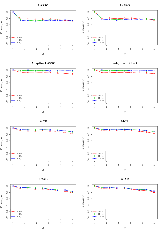
Figure 1: Regression case (Example 1): $n=200$, $p=8$, $\boldsymbol{\beta}=(3,1.5,2,0,0,0,0,0)^{\intercal}.$ $\mathbf{x}_{i}$ for $i=1,\ldots,n$ are i.i.d. from $N_{p}(0,\boldsymbol{I})$. The first column presents the results for $F$-measure, the second column is for $G$-measure.

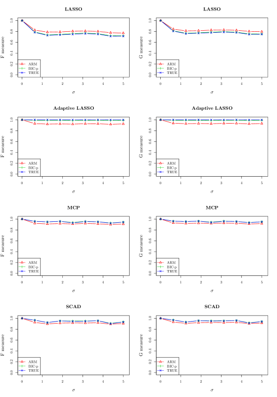
Figure 2: Regression case (Example 2): $n=1000$, $p=8$, $\boldsymbol{\beta}=(3,1.5,2,0,0,0,0,0)^{\intercal}.$ $\mathbf{x}_{i}$ for $i=1,\ldots,n$ are i.i.d. from $N_{p}(0,\boldsymbol{I})$. The first column presents the results for $F$-measure, the second column is for $G$-measure.

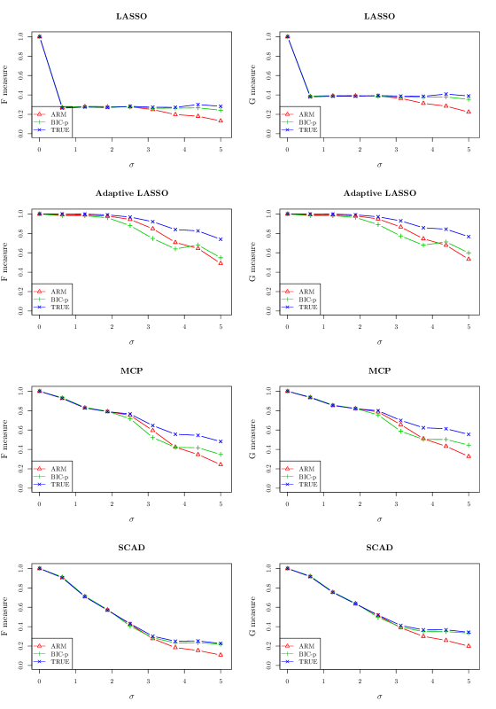
Figure 3: Regression case (Example 3): $n=200$, $p=2000$, $\boldsymbol{\beta}=(\beta_{1},\ldots,\beta_{p})^{\intercal}$, where $(\beta_{1},\beta_{2},\beta_{3})=(3,1.5,2)$ and $(\beta_{4},\ldots,\beta_{2000})$ are zeros. $\mathbf{x}_{i}$ for $i=1,\ldots,n$ are i.i.d. from $N(0,\boldsymbol{I}_{p})$. The first column presents the results for $F$-measure, the second column is for $G$-measure.

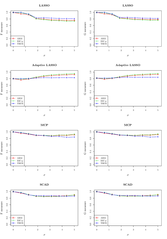
Figure 4: Regression case (Example 4): $n=200$, $p=30$, the components 1–5 of $\boldsymbol{\beta}$ are 10.5, components 6–10 are 5.5, components 11–15 are 0.5 and the rests are zeros. $\mathbf{x}_{i}$ for $i=1,\ldots,n$ are from $X\sim N_{p}(0,\boldsymbol{\Sigma})$ with $\boldsymbol{\Sigma}=(0.4^{|j-k|})_{p\times p}$. The first column presents the results for $F$-measure, the second column is for $G$-measure.

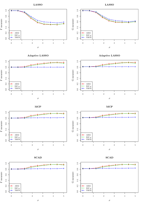
Figure 5: Regression case (Example 5): $n=200$, $p=200$, the components 1–5 of $\beta$ are 10.5, the components 6–10 are 5.5, the components 11–15 are 0.5 and the rests are zeros. $\mathbf{x}_{i}$ for $i=1,\ldots,n$ are from $X\sim N_{p}(0,\boldsymbol{\Sigma})$. The first 15 predictors $(X_{1},\ldots,X_{15})$ and the remaining 185 predictors $(X_{16},\ldots,X_{200})$ are independent. The correlation between $X_{j}$ and $X_{k}$ in $(X_{1},\ldots,X_{15})$ is $0.4^{|j-k|}$. The correlation between $X_{j}$ and $X_{k}$ in $(X_{16},\ldots,X_{200})$ is $0.4^{|j-k|}$. The first column presents the results for $F$-measure, the second column is for $G$-measure.

In Figure 5, the over-estimation in SCAD and MCP, when $\sigma$ is large, is due to highly weighted candidate models miss several small coefficients variables, which is caused by the decaying coefficients and worsened by correlation between the variables. While for Lasso, when $\sigma$ is small, PAVI can find good candidate models to put high weights on, thus the estimation is good; when $\sigma$ is larger, the candidate models with high weights miss several true variables. At the same time, Lasso chooses more redundant variables when $\sigma$ becomes larger. Therefore, the precision is under-estimated, so does the $F$-measure.

6.   REAL DATA

In this section, we apply PAVI to several model selection methods using gene expression data for cancer-related biomarker identification. The biomarker selection process is usually under high-dimensional, small-sample, and high-noise setting with highly-correlated genes involved (Golub et al., 1999; West et al., 2001; Ma and Huang, 2008; Ang et al., 2016). As such, the sets of genes identified may be subject to substantial changes due to small perturbations in the data (Baggerly et al., 2004; Meinshausen and Bühlmann, 2010; Henry and Hayes, 2012; Nan and Yang, 2014; Lim and Yu, 2016; Stodden, 2015). Here we use $\widehat{F}$ and $\widehat{G}$ to evaluate such selection uncertainty.

Our goal is to provide a serious and careful analysis of outcomes of variable selection methods from multiple angles to understand the key issues of interest. One may wonder if any strong statement can be said because no one knows the truth. We hope our analysis provides strong enough evidence that the estimated $F$ and $G$ values yield valuable information.

6.1.   Data description

We consider three well-studied benchmark cancer datasets: Colon (Alon et al., 1999), Leukemia (Golub et al., 1999) and Prostate (Singh et al., 2002). Table 6 provides a brief summary.

Table 6: Summary of Colon, Leukemia, Prostate. In Colon, $y=1$ represents colon tumor samples and $y=0$ represents normal colon tissue samples; In Leukemia, $y=1$ represents acute myeloblastic leukemia samples and $y=0$ represents acute lymphoblastic leukemia samples; In Prostate, $y=1$ represents tumor samples and $y=0$ represents normal prostate samples.

Data	$n$	$n_{1}$	$n_{2}$	$p$	Data source
		($y=1$)	($y=0$)	(number of genes)
Colon	62	40	22	2000	Alon et al. (1999)
Leukemia	72	25	47	7129	Golub et al. (1999)
Prostate	102	52	50	12600	Singh et al. (2002)

6.2.   Methods/models to be examined

On these three datasets, we compare the variable selection performance of four commonly used penalized regression methods: Lasso, adaptive Lasso, MCP and SCAD. We first obtain the final model $\mathcal{A}^{0}$ for each method (the tuning parameter $\lambda$ is selected using five-fold cross-validation). Then we use PAVI to estimate $\widehat{F}(\mathcal{A}^{0})$ and $\widehat{G}(\mathcal{A}^{0})$ with two weightings, ARM and BIC-p. The whole procedure is repeated 100 times to average out randomness in the tuning parameter selection, and the averages of $\widehat{F}(\mathcal{A}^{0})$, $\mathrm{sd}\big{(}\widehat{F}(\mathcal{A}^{0})\big{)}$ and $\widehat{G}(\mathcal{A}^{0})$, $\mathrm{sd}\big{(}\widehat{G}(\mathcal{A}^{0})\big{)}$ are summarized in Tables 7, 8 and 9. For comparison, we also include several other models studied in the existing literature. Specifically, we consider Leung and Hung, 2010 (L10), Yang and Song, 2010 (Y10), Chandra and Gupta, 2011 (C11) and Lee and Leu, 2011 (L11) for Colon, Leung and Hung, 2010 (L10), Yang and Song, 2010 (Y10), and Ji et al., 2011 (J11; two kinds of models are provided via different importance criterion in this work, denoted by J11¹ and J11² hereafter respectively) for Leukemia, and Leung and Hung, 2010 (L10) and Sharma et al., 2012 (S12) for Prostate.

Y10, J11 and S12 used linear-based variable selection techniques without initial variable screening. Specifically, Y10 used the probit regression model; J11 used the linear kernel support vector classifier (SVC); S12 used the linear discriminant analysis (LDA) technique with nearest centroid classifier (NCC). In contrast, L10, C11 and L11 used nonparametric variable selection techniques: L10 used SVM; C11 used the naïve Bayes classifier (NBC) and SVM; L11 used the support vector machine (SVM). In addition, we consider the Importance Screening method (ImpS) by Ye et al. (2016), which uses a sparsity oriented importance learning for variable screening.

6.3.   Results

The estimated $\widehat{F}$ and $\widehat{G}$ of each model on Colon, Leukemia and Prostate are reported in Tables 7, 8 and 9 respectively. We find that ImpS achieves almost the largest estimated $\widehat{F}$ and $\widehat{G}$ on all three data sets. L10 has basically zero $\widehat{F}$ and $\widehat{G}$ for Colon and Prostate. J11¹ and J11² has basically zero $\widehat{F}$ and $\widehat{G}$ for Leukemia. (These cases are bolded in Tables 7, 8 and 9.) This suggests that, from a logistic regression modeling perspective, they may have chosen “wrong” variables and they have very low recalls or precisions.

Table 7: Estimated $F$- and $G$-measures and standard deviations for Colon. L10 has numerically zero $\widehat{F}$ and $\widehat{G}$ values (bolded in the Table).

	ARM					BIC-p
	$F$	$sd.F$	$G$	$sd.G$		$F$	$sd.F$	$G$	$sd.G$
Lasso	0.147	0.024	0.280	0.022		0.205	0.066	0.332	0.058
AdLasso	0.194	0.165	0.255	0.211		0.309	0.191	0.361	0.209
MCP	0.349	0.045	0.459	0.035		0.460	0.130	0.544	0.093
SCAD	0.149	0.032	0.274	0.039		0.211	0.074	0.331	0.071
ImpS	0.524	0.081	0.596	0.065		0.656	0.176	0.698	0.118
L11	0.111	0.110	0.175	0.175		0.112	0.105	0.157	0.151
Y10	0.103	0.017	0.233	0.018		0.146	0.048	0.276	0.047
C11	0.184	0.020	0.317	0.022		0.223	0.076	0.333	0.082
L10	0.000	0.000	0.000	0.000		0.000	0.000	0.000	0.000

Table 8: Estimated $F$- and $G$-measures and standard deviations for Leukemia. J11¹ and J11² have numerically zero $\widehat{F}$ and $\widehat{G}$ values (bolded in the Table).

	ARM					BIC-p
	$F$	$sd.F$	$G$	$sd.G$		$F$	$sd.F$	$G$	$sd.G$
Lasso	0.083	0.025	0.206	0.026		0.079	0.012	0.203	0.014
AdLasso	0.323	0.044	0.432	0.031		0.322	0.039	0.434	0.033
MCP	0.168	0.170	0.221	0.210		0.061	0.089	0.078	0.108
SCAD	0.094	0.028	0.220	0.028		0.090	0.013	0.216	0.015
ImpS	0.525	0.065	0.591	0.042		0.573	0.129	0.636	0.102
$\mathrm{J11}^{1}$	0.000	0.000	0.000	0.000		0.000	0.000	0.000	0.000
$\mathrm{J11}^{2}$	0.000	0.000	0.000	0.000		0.000	0.000	0.000	0.000
Y10	0.108	0.014	0.236	0.009		0.105	0.002	0.233	0.012
L10	0.212	0.180	0.265	0.224		0.336	0.089	0.419	0.110

Table 9: Estimated $F$- and $G$-measures and standard deviations for Prostate. L10 has numerically zero $\widehat{F}$ and $\widehat{G}$ values (bolded in the Table).

	ARM					BIC-p
	$F$	$sd.F$	$G$	$sd.G$		$F$	$sd.F$	$G$	$sd.G$
Lasso	0.064	0.004	0.181	0.005		0.064	0.003	0.181	0.004
AdLasso	0.190	0.011	0.323	0.009		0.189	0.008	0.323	0.007
MCP	0.018	0.019	0.027	0.022		0.018	0.012	0.027	0.014
SCAD	0.097	0.006	0.225	0.007		0.096	0.005	0.225	0.005
ImpS	0.333	0.011	0.447	0.008		0.333	0.012	0.447	0.009
S12	0.395	0.037	0.494	0.047		0.400	0.003	0.500	0.007
L10	0.000	0.000	0.000	0.000		0.000	0.000	0.000	0.000

6.4.   Are the zero $\widehat{F}$ and $\widehat{G}$ values too harsh for the methods?

It is striking that the $\widehat{F}$ and $\widehat{G}$ for some selections are numerically zero, which seems rather extreme. Does this mean those models are truly poor or rather our performance assessment methodology fails? We would like to examine the matter from three perspectives.

6.4.1 First perspective: the labels of the selected genes

First, let us examine the labels of the selected genes. We obtain the selected genes in the literature. And we use five-fold cross-validation in penalization parameter tuning to obtain selected genes for the penalized regression models. In Tables 10, 11 and 12, the results show that the genes selected by L10 (Colon and Prostate), J11¹ and J11² (Leukemia) are mostly not supported by other models. More specifically, the choices of variables by L10, J11¹ and J11² in those cases respectively share zero, one or at most two genes with the other methods. (These cases are underlined in Tables 10, 11 and 12.)

Table 10: Labels of selected genes for Colon.

	Labels of selected genes
Lasso	{66, 249, 377, 493, 765, 1325, 1346, 1423, 1582, 1644, 1772, 1870}
AdLasso	{249, 377, 765, 1582, 1772, 1870}
MCP	{249, 377, 1644, 1772, 1870}
SCAD	{377, 617, 765, 1024, 1325, 1346, 1482, 1504, 1582, 1644, 1772, 1870}
ImpS	{249, 1772}
L11	{249, 286, 765, 1058, 1485, 1671, 1771, 1836}
Y10	{14, 161, 249, 377, 492, 493, 576, 792, 822, 1042, 1210,
	1346, 1400, 1423, 1549, 1635, 1772, 1843, 1924}
C11	{249, 399, 513, 515, 780, 1042, 1325, 1582, 1771, 1772}
L10	{732, 994, 1473, 1763, 1794, 1843}

Table 11: Labels of selected genes for Leukemia.

	Labels of selected genes
Lasso	{804, 1239, 1674, 1745, 1779, 1796, 1834, 1882, 1928, 1933,
	1941, 2121, 2288, 3847, 4196, 4328, 4847, 4951, 4973, 5002,
	5107, 5335, 5766, 6055, 6169, 6539, 6855}
AdLasso	{1779, 1834, 4328, 4847, 4951}
MCP	{804, 1941, 3837, 4714, 4847, 4951, 6539}
SCAD	{804, 1674, 1745, 1779, 1834, 1882, 1928, 1941, 2288, 3847, 4196,
	4328, 4847, 4951, 4973, 5002, 5766, 5772, 6169, 6225, 6281, 6539, 6855}
ImpS	{1239, 4847, 4951}
$\mathrm{J11}^{1}$	{1376, 1394, 1674, 1882, 2186, 2402, 6200, 6201, 6803}
$\mathrm{J11}^{2}$	{1394, 1674, 1882, 2186, 5976, 6200, 6201, 6806}
Y10	{760, 804, 1745, 1829, 1834, 1882, 2354, 3320, 4052,
	4211, 4377, 4535, 4847, 5039, 6041, 6218, 6376, 6540}
L10	{220, 1086, 1834, 2020}

Table 12: Labels of selected genes for Prostate.

	Labels of selected genes
Lasso	{1107, 3617, 4282, 4438, 4525, 4636, 5661, 5838, 5890, 6145, 6185,
	6838, 7375, 7428, 7539, 7623, 7915, 8123, 8965, 9034, 9093, 9816,
	9850, 10234, 10537, 10956, 11858, 11871, 12153, 12462}
AdLasso	{5661, 5890, 6185, 7539, 7623, 8965, 9034, 9093, 10234, 11858}
MCP	{7623, 7924, 8965, 9034, 9816, 10234, 11858}
SCAD	{1107, 3540, 4636, 5661, 5838, 5890, 6185, 7623, 8603, 8965, 9034,
	9093, 9816, 10234, 10956, 11858, 11871, 12153}
ImpS	{8965, 9034, 10234, 11858}
S12	{4377, 6185, 6390, 6915}
L10	{4743, 6096, 8475, 9575, 9927, 12331}

6.4.2 Second perspective: predictive accuracy

Secondly, we would like to examine the issue from a predictive accuracy perspective. We randomly split the dataset into 4/5 observations for training and 1/5 observations for testing. We fit the SVM models with those selected genes on the training data using kernlab (Karatzoglou et al., 2004) and evaluate the predictive accuracy on the testing data. The whole procedure is repeated 100 times and the averaged classification accuracy and “standard errors” (w.r.t. the permutations) are recorded in Table 13. Alternatively, we may consider the parametric models. We fit the logistic regression with the genes selected (in Table 13). We find that L10, J11¹ and J11² have worse predictive accuracy (bolded in Table 13) compared with the simpler model by ImpS, which adds evidence to support the validity of their low $\widehat{F}$ and $\widehat{G}$ values.

Table 13: Comparisons of classification accuracy on Colon, Leukemia, and Prostate using logistic regression and SVM, respectively.

Logistic Model
Colon			Leukemia			Prostate
ImpS	86.3 (0.8)		ImpS	97.1 (0.3)		ImpS	94.0 (0.4)
Lasso	80.0 (1.0)		Lasso	99.8 (0.1)		Lasso	97.0 (0.4)
AdLasso	85.5 (0.8)		AdLasso	93.9 (0.5)		AdLasso	99.8 (0.1)
MCP	85.1 (0.8)		MCP	99.5 (0.1)		MCP	98.7 (0.2)
SCAD	84.3 (0.8)		SCAD	97.9 (0.3)		SCAD	97.1 (0.2)
L11	80.4 (0.8)		$\mathrm{J11}^{1}$	89.4 (0.8)		S12	96.5 (0.4)
Y10	90.9 (0.9)		$\mathrm{J11}^{2}$	89.8 (0.7)		L10	59.0 (0.8)
C11	79.6 (1.0)		Y10	91.2 (0.7)
L10	83.0 (0.9)		L10	95.5 (0.4)
SVM Model
Colon			Leukemia			Prostate
ImpS	84.0 (0.9)		ImpS	97.6 (0.3)		ImpS	95.3 (0.4)
Lasso	75.8 (0.9)		Lasso	99.1 (0.2)		Lasso	96.3 (0.4)
AdLasso	79.0 (0.9)		AdLasso	95.8 (0.4)		AdLasso	96.6 (0.3)
MCP	83.1 (1.1)		MCP	99.0 (0.2)		MCP	97.1 (0.3)
SCAD	86.0 (0.9)		SCAD	99.1 (0.2)		SCAD	96.4 (0.3)
L11	79.0 (1.1)		$\mathrm{J11}^{1}$	88.6 (0.8)		S12	95.5 (0.4)
Y10	78.3 (1.0)		$\mathrm{J11}^{2}$	87.4 (0.9)		L10	59.3 (0.9)
C11	77.1 (0.9)		Y10	90.2 (0.6)
L10	72.4 (0.9)		L10	92.2 (0.6)

6.4.3 Third perspective: traditional model fitting

For the third perspective, we investigate the AIC, BIC, and deviance measures. When comparing models fitted by maximum likelihood to the same data, the smaller the AIC or BIC value is, the better the model fits, from their respective stand points.

Table 14: Estimated AIC, BIC and deviance for Colon, Leukemia and Prostate.

Colon					Leukemia					Prostate
	AIC	BIC	Dev.			AIC	BIC	Dev.			AIC	BIC	Dev.
Lasso	26.0	53.6	0.0			56.0	119.7	0.0			62.0	143.3	0.0
AdLasso	34.9	49.8	20.9			12.0	25.6	0.0			22.0	50.8	0.0
MCP	32.1	44.9	20.1			16.0	34.2	0.0			16.0	36.9	0.0
SCAD	26.0	53.6	0.0			48.0	102.6	0.0			38.0	87.8	0.0
ImpS	35.5	44.1	27.5			8.0	17.1	0.0			12.0	27.7	9.4
L11	51.4	70.5	33.4		J$11^{1}$	20.0	42.7	0.0		S12	36.1	49.2	26.1
Y10	40.0	82.5	0.0		J$11^{2}$	18.0	38.4	0.0		L10	140.1	158.5	126.1
C11	45.2	68.6	23.2		Y10	38.0	81.2	0.0
L10	48.6	63.5	34.6		L10	10.0	21.3	0.0

From Table 14, the model for Colon with zero $\widehat{F}$ and $\widehat{G}$ values also has relatively large AIC, BIC and deviance values (bolded in the Table) compared to the models with large $\widehat{F}$ and $\widehat{G}$ values. The results are similar for the other two data sets, except that the deviance values for Leukemia are extremely small due to easy classification nature of the data.

In summary, we see that the low (near zero) $\widehat{F}$ and $\widehat{G}$ values for the investigated sets of selected genes above are supported from the three perspectives. Our PAVI approach provides a valid tool for checking the reliability and reproducibility of a given set of selected variables when the true model is not known. To be fair, we want to emphasize that the poor $\widehat{F}$ and $\widehat{G}$ values of some of the selection methods are based on the logistic regression perspective, although Table 13 seems to suggest that logistic regression works at least as well as SVM.

7.   CONCLUSION

There are many variable selection methods, but so far most of investigations on their behaviors are limited to theoretical studies and somewhat scattered simulation results, which may have little to do with a specific dataset at hand. There is a severe lack of valid performance measures that are computable based on data alone. This leads to the pessimistic view that “For real data, nothing can be said strongly about which method is better for describing the data generation mechanism since no one knows the truth.” Sound implementable variable selection diagnostic tools can shed a positive light on the matter.

Nan and Yang (2014) proposed an approach to gain insight on how many variables are likely missed and how many are not quite justifiable for an outcome of a variable selection process. In real applications, it is often of interest and important to summarize the two types of selection errors into a single measure to characterize the behavior of a variable selection method. Due to this reason, $F$- and $G$-measures are gaining popularity in model selection literature. If we are given a data set for which several model selection methods are considered, prior to this work, the available model diagnostic tools can only tell us (a) Which methods are more unstable; (b) How many terms are likely missed or unsupported. This information, unlike the $F$- and $G$-measures, may not be enough to give one a good sense of the overall model selection performance. In this paper, we have advanced the line of research on model selection diagnostics by providing a valid estimation of $F$- and $G$-measures.

We have proved that the estimated $F$- and $G$-measures are uniformly consistent as long as the weighting is weakly consistent. The simulation results clearly show that the $\widehat{F}$ and $\widehat{G}$ based on our PAVI approach nicely characterizes the overall performance of the model selection outcomes. The information can be utilized for comparing different methods for the data at hand.

We have used three real data examples to demonstrate the utility of our PAVI methodology. There have been many variable selection results reported in the literature on these data sets. A careful study with multiple perspectives has provided strong evidence to suggest that some of the variable selection outcomes may be far away from the best set of variables to use for logistic regression or SVM with the given information.

Appendix for “Performance Assessment of High-dimensional Variable Identification”

In this appendix we provide technical proofs for the theorems and lemmas in “Performance Assessment of High-dimensional Variable Identification”.

Proof of Theorem 1

Part I: $F$-measure

Proof.

Denote by $\nabla$ the symmetric difference between two sets. Estimated $F$-measure can be rewritten as

$$\widehat{F}(\mathcal{A}^{0})=\sum w_{k}F(\mathcal{A}^{0};\mathcal{A}^{k}),\qquad F(\mathcal{A}^{0};\mathcal{A}^{k})=\frac{|\mathcal{A}^{0}|+|\mathcal{A}^{k}|-|\mathcal{A}^{0}\nabla\mathcal{A}^{k}|}{|\mathcal{A}^{0}|+|\mathcal{A}^{k}|}.$$

We have

$$|\widehat{F}(\mathcal{A}^{0})-F(\mathcal{A}^{0})| =\left|\sum w_{k}F(\mathcal{A}^{0};\mathcal{A}^{k})-F(\mathcal{A}^{0})\right|$$

$$=\left|\sum w_{k}(F(\mathcal{A}^{0};\mathcal{A}^{k})-F(\mathcal{A}^{0}))\right|\leq\sum w_{k}|F(\mathcal{A}^{0};\mathcal{A}^{k})-F(\mathcal{A}^{0})|$$

$$=\sum w_{k}\left|1-\frac{|\mathcal{A}^{0}\nabla\mathcal{A}^{k}|}{|\mathcal{A}^{0}|+|\mathcal{A}^{k}|}-1+\frac{|\mathcal{A}^{0}\nabla\mathcal{A}^{*}|}{|\mathcal{A}^{0}|+|\mathcal{A}^{*}|}\right|$$

$$=\sum w_{k}\left|\frac{|\mathcal{A}^{0}|\cdot(|\mathcal{A}^{0}\nabla\mathcal{A}^{*}|-|\mathcal{A}^{0}\nabla\mathcal{A}^{k}|)+|\mathcal{A}^{k}|\cdot|\mathcal{A}^{0}\nabla\mathcal{A}^{*}|-|\mathcal{A}^{*}|\cdot|\mathcal{A}^{0}\nabla\mathcal{A}^{k}|}{(|\mathcal{A}^{0}|+|\mathcal{A}^{k}|)(|\mathcal{A}^{0}|+|\mathcal{A}^{*}|)}\right|$$

$$\leq\text{$\underbrace{\sum w_{k}\frac{|\mathcal{A}^{0}|\cdot||\mathcal{A}^{0}\nabla\mathcal{A}^{*}|-|\mathcal{A}^{0}\nabla\mathcal{A}^{k}||}{(|\mathcal{A}^{0}|+|\mathcal{A}^{k}|)(|\mathcal{A}^{0}|+|\mathcal{A}^{*}|)}}_{A}$+$\underbrace{\sum w_{k}\frac{|\mathcal{A}^{k}|\cdot||\mathcal{A}^{0}\nabla\mathcal{A}^{*}|-|\mathcal{A}^{0}\nabla\mathcal{A}^{k}||}{(|\mathcal{A}^{0}|+|\mathcal{A}^{k}|)(|\mathcal{A}^{0}|+|\mathcal{A}^{*}|)}}_{B}$}$$

$$+\underbrace{\sum w_{k}\frac{||\mathcal{A}^{k}|-|\mathcal{A}^{*}||\cdot|\mathcal{A}^{0}\nabla\mathcal{A}^{k}|}{(|\mathcal{A}^{0}|+|\mathcal{A}^{k}|)(|\mathcal{A}^{0}|+|\mathcal{A}^{*}|)}}_{C}.$$

For ease of notation, we divide the right-most hand side of the above inequality into three parts and denote them by $A$, $B$, and $C$ respectively. Note that since $\left||\mathcal{A}^{0}\nabla\mathcal{A}^{*}|-|\mathcal{A}^{0}\nabla\mathcal{A}^{k}|\right|\leq|\mathcal{A}^{*}\nabla\mathcal{A}^{k}|$, we have

$$A\leq\sum w_{k}\frac{|\mathcal{A}^{0}|\cdot|\mathcal{A}^{*}\nabla\mathcal{A}^{k}|}{(|\mathcal{A}^{0}|+|\mathcal{A}^{k}|)(|\mathcal{A}^{0}|+|\mathcal{A}^{*}|)}\leq\sum w_{k}\frac{|\mathcal{A}^{*}\nabla\mathcal{A}^{k}|}{|\mathcal{A}^{*}|}.$$

Similarly, it can be shown that

$$B\leq\sum w_{k}\frac{|\mathcal{A}^{*}\nabla\mathcal{A}^{k}|}{|\mathcal{A}^{*}|}.$$

Let us now prove a similar bound also holds for $C.$ Specifically, we have

$$C =\sum w_{k}\frac{||\mathcal{A}^{k}|-|\mathcal{A}^{*}||\cdot|\mathcal{A}^{0}\nabla\mathcal{A}^{k}|}{(|\mathcal{A}^{0}|+|\mathcal{A}^{k}|)(|\mathcal{A}^{0}|+|\mathcal{A}^{*}|)}\leq\sum w_{k}\frac{\left||\mathcal{A}^{k}|-|\mathcal{A}^{*}|\right|}{|\mathcal{A}^{0}|+|\mathcal{A}^{*}|}$$

$$=\sum w_{k}\frac{\left|(|\mathcal{A}^{k}\backslash\mathcal{A}^{*}|+|\mathcal{A}^{k}\cap\mathcal{A}^{*}|)-(|\mathcal{A}^{*}\backslash\mathcal{A}^{k}|+|\mathcal{A}^{k}\cap\mathcal{A}^{*}|)\right|}{|\mathcal{A}^{0}|+|\mathcal{A}^{*}|}$$

$$=\sum w_{k}\frac{\left||\mathcal{A}^{k}\backslash\mathcal{A}^{*}|-|\mathcal{A}^{*}\backslash\mathcal{A}^{k}|\right|}{|\mathcal{A}^{0}|+|\mathcal{A}^{*}|}\leq\sum w_{k}\frac{|\mathcal{A}^{k}\backslash\mathcal{A}^{*}|+|\mathcal{A}^{*}\backslash\mathcal{A}^{k}|}{|\mathcal{A}^{0}|+|\mathcal{A}^{*}|}$$

$$=\sum w_{k}\frac{|\mathcal{A}^{k}\nabla\mathcal{A}^{*}|}{|\mathcal{A}^{0}|+|\mathcal{A}^{*}|}\leq\sum w_{k}\frac{|\mathcal{A}^{k}\nabla\mathcal{A}^{*}|}{|\mathcal{A}^{*}|}.$$

It follows that for any $\mathcal{A}^{0}$ in $\mathbb{C}$

$$|\widehat{F}(\mathcal{A}^{0})-F(\mathcal{A}^{0})|\leq A+B+C\leq 3\sum w_{k}\frac{|\mathcal{A}^{*}\nabla\mathcal{A}^{k}|}{|\mathcal{A}^{*}|}.$$

Therefore,

$$\sup_{\mathcal{A}^{0}\in\mathbb{C}}|\widehat{F}(\mathcal{A}^{0})-F(\mathcal{A}^{0})|\leq 3\sum w_{k}\frac{|\mathcal{A}^{*}\nabla\mathcal{A}^{k}|}{|\mathcal{A}^{*}|}.$$

Now under the assumption that the model weighting $w$ is weakly consistent,

$$\sum w_{k}\frac{|\mathcal{A}^{*}\nabla\mathcal{A}^{k}|}{|\mathcal{A}^{*}|}\overset{p}{\rightarrow}0.$$

We have proved $\sup_{\mathcal{A}^{0}\in\mbox{$\mathbb{C}$}}|\widehat{F}(\mathcal{A}^{0})-F(\mathcal{A}^{0})|\overset{p}{\rightarrow}0.$ ∎

Part II: $G$-measure

Proof.

For a given $\mathcal{A}^{0}$ in $\mathbb{C}$, the estimated $G$-measure can be rewritten as

$$\widehat{G}(\mathcal{A}^{0})=\sum w_{k}G(\mathcal{A}^{0};\mathcal{A}^{k}),\qquad G(\mathcal{A}^{0};\mathcal{A}^{k})=\frac{|\mathcal{A}^{0}|+|\mathcal{A}^{k}|-|\mathcal{A}^{0}\nabla\mathcal{A}^{k}|}{2\sqrt{|\mathcal{A}^{0}|\cdot|\mathcal{A}^{k}|}}.$$

Suppose $|\widehat{G}(\mathcal{A}^{0})-G(\mathcal{A}^{0})|$ does not converge to $0$ in probability uniformly over $\mathbb{C}$, then there exist some subsequence $n_{1},n_{2},\cdots$, $\epsilon_{1}>0,\delta>0$, $\mathcal{A}^{0}_{n_{j}}\in\mathbb{C}$, and sets $\mathcal{S}_{n_{j}}$, s.t. $P(\mathcal{S}_{n_{j}})\geq\delta$ and $|\widehat{G}(\mathcal{A}^{0}_{n_{j}})-G(\mathcal{A}^{0}_{n_{j}})|>\epsilon_{1}$ on $\mathcal{S}_{n_{j}}.$ For ease of notation, we denote $\mathcal{A}^{0}_{n_{j}}$ as $\mathcal{A}^{0}$ in the following proof.

With the above, we first prove that we must have $\frac{|\mathcal{A}^{0}|}{|\mathcal{A}^{*}|}\overset{p}{\rightarrow}$0 on $\mathcal{S}_{n_{j}}$ as $n_{j}\rightarrow\infty$. If not, then there exist $\epsilon_{2}>0,$ a subsequence $n_{j_{l}}$ and sets $\mathcal{N}_{n_{j_{l}}}$ such that on $\mathcal{N}_{n_{j_{l}}}$ we have $\frac{|\mathcal{A}^{0}|}{|\mathcal{A}^{*}|}>\epsilon_{2}>0$. Then we can actually prove $|\widehat{G}(\mathcal{A}^{0})-G(\mathcal{A}^{0})|\overset{p}{\longrightarrow}0$ on $\mathcal{N}_{n_{j_{l}}}$ as follows.

By definition of $\widehat{G}$ and $G$, and $\frac{|\mathcal{A}^{0}|}{|\mathcal{A}^{*}|}>\epsilon_{2}>0$ on $\mathcal{N}_{n_{j_{l}}}$, we have

$$|\widehat{G}(\mathcal{A}^{0})-G(\mathcal{A}^{0})| =|\sum w_{k}G(\mathcal{A}^{0};\mathcal{A}^{k})-G(\mathcal{A}^{0})|$$

$$\leq\sum w_{k}|G(\mathcal{A}^{0};\mathcal{A}^{k})-G(\mathcal{A}^{0})|$$

$$=\sum w_{k}\left|\frac{|\mathcal{A}^{0}|+|\mathcal{A}^{k}|-|\mathcal{A}^{0}\nabla\mathcal{A}^{k}|}{2\sqrt{|\mathcal{A}^{0}|\cdot|\mathcal{A}^{k}|}}-\frac{|\mathcal{A}^{0}|+|\mathcal{A}^{*}|-|\mathcal{A}^{0}\nabla\mathcal{A}^{*}|}{2\sqrt{|\mathcal{A}^{0}|\cdot|\mathcal{A}^{*}|}}\right|$$

$$\leq\sum w_{k}\frac{|\sqrt{|\mathcal{A}^{*}|}-\sqrt{|\mathcal{A}^{k}|}|\cdot||\mathcal{A}^{0}|+|\mathcal{A}^{k}|-|\mathcal{A}^{0}\nabla\mathcal{A}^{k}||}{2\sqrt{|\mathcal{A}^{*}|\cdot|\mathcal{A}^{0}|\cdot|\mathcal{A}^{k}|}}$$

$$+\sum w_{k}\frac{\sqrt{|\mathcal{A}^{k}|}\cdot||\mathcal{A}^{k}|-|\mathcal{A}^{*}|+|\mathcal{A}^{0}\nabla\mathcal{A}^{*}|-|\mathcal{A}^{0}\nabla\mathcal{A}^{k}||}{2\sqrt{|\mathcal{A}^{*}|\cdot|\mathcal{A}^{0}|\cdot|\mathcal{A}^{k}|}}$$

$$\leq\underbrace{\sum w_{k}\frac{|\sqrt{|\mathcal{A}^{*}|}-\sqrt{|\mathcal{A}^{k}|}|\cdot||\mathcal{A}^{0}|+|\mathcal{A}^{k}|-|\mathcal{A}^{0}\nabla\mathcal{A}^{k}||}{2\sqrt{|\mathcal{A}^{*}|\cdot|\mathcal{A}^{0}|\cdot|\mathcal{A}^{k}|}}}_{A}$$

$$+\underbrace{\sum w_{k}\frac{||\mathcal{A}^{k}|-|\mathcal{A}^{*}||}{2\sqrt{|\mathcal{A}^{*}|\cdot|\mathcal{A}^{0}|}}}_{B}+\underbrace{\sum w_{k}\frac{||\mathcal{A}^{0}\nabla\mathcal{A}^{*}|-|\mathcal{A}^{0}\nabla\mathcal{A}^{k}||}{2\sqrt{|\mathcal{A}^{*}|\cdot|\mathcal{A}^{0}|}}}_{C}.$$

For notational convenience, we divide the right-most-hand side of the above inequality into three parts and denote them by $A$, $B$, and $C$ respectively. For part $A$, because $|\mathcal{A}^{0}|+|\mathcal{A}^{k}|-|\mathcal{A}^{0}\nabla\mathcal{A}^{k}|=2|\mathcal{A}^{0}\cap\mathcal{A}^{k}|$ and $\left||\mathcal{A}^{*}|-|\mathcal{A}^{k}|\right|\leq|\mathcal{A}^{*}\nabla\mathcal{A}^{k}|$, together with $|\mathcal{A}^{0}\cap\mathcal{A}^{k}|\leq\sqrt{|\mathcal{A}^{0}|\cdot|\mathcal{A}^{k}|}$, we have

$$A=\sum w_{k}\frac{\left||\mathcal{A}^{*}|-|\mathcal{A}^{k}|\right|\cdot|\mathcal{A}^{0}\cap\mathcal{A}^{k}|}{\left(\sqrt{|\mathcal{A}^{*}|}+\sqrt{|\mathcal{A}^{k}|}\right)\sqrt{|\mathcal{A}^{*}|\cdot|\mathcal{A}^{0}|\cdot|\mathcal{A}^{k}|}}\leq\sum w_{k}\frac{|\mathcal{A}^{*}\nabla\mathcal{A}^{k}|}{|\mathcal{A}^{*}|}.$$

For part $B$, since $||\mathcal{A}^{k}|-|\mathcal{A}^{*}||\leq|\mathcal{A}^{k}\nabla\mathcal{A}^{*}|$ and $\frac{|\mathcal{A}^{0}|}{|\mathcal{A}^{*}|}>\epsilon_{2}>0$ on $\mathcal{N}_{n_{j_{l}}}$, we have

$$B=\sum w_{k}\frac{\left||\mathcal{A}^{k}|-|\mathcal{A}^{*}|\right|}{2\sqrt{|\mathcal{A}^{*}|\cdot|\mathcal{A}^{0}|}}\leq\frac{1}{2\sqrt{\epsilon_{2}}}\sum w_{k}\frac{|\mathcal{A}^{k}\nabla\mathcal{A}^{*}|}{|\mathcal{A}^{*}|}.$$

For part $C$, it follows from the facts that $||\mathcal{A}^{0}\nabla\mathcal{A}^{*}|-|\mathcal{A}^{0}\nabla\mathcal{A}^{k}||\leq|\mathcal{A}^{*}\nabla\mathcal{A}^{k}|$ and that $\frac{|\mathcal{A}^{0}|}{|\mathcal{A}^{*}|}>\epsilon_{2}>0$ on $\mathcal{N}_{n_{j_{l}}}$, we have

$$C=\sum w_{k}\frac{||\mathcal{A}^{0}\nabla\mathcal{A}^{*}|-|\mathcal{A}^{0}\nabla\mathcal{A}^{k}||}{2\sqrt{|\mathcal{A}^{*}|\cdot|\mathcal{A}^{0}|}}\leq\frac{1}{2\sqrt{\epsilon_{2}}}\frac{\sum w_{k}|\mathcal{A}^{*}\nabla\mathcal{A}^{k}|}{|\mathcal{A}^{*}|}.$$

Consequently, we have that on $\mathcal{N}_{n_{j_{l}}}$,

$$|\widehat{G}(\mathcal{A}^{0})-G(\mathcal{A}^{0})|\leq A+B+C\leq(1+\frac{1}{\sqrt{\epsilon_{2}}})\sum w_{k}\frac{|\mathcal{A}^{*}\nabla\mathcal{A}^{k}|}{|\mathcal{A}^{*}|}.$$

Under the assumption that the model weighting $w$ is weakly consistent,

$$\sum w_{k}\frac{|\mathcal{A}^{*}\nabla\mathcal{A}^{k}|}{|\mathcal{A}^{*}|}\overset{p}{\rightarrow}0,$$

we must have $|\widehat{G}(\mathcal{A}^{0})-G(\mathcal{A}^{0})|\overset{p}{\rightarrow}0$ on $\mathcal{N}_{n_{j_{l}}}$. This contradicts with the statement that $|\widehat{G}(\mathcal{A}^{0})-G(\mathcal{A}^{0})|>\epsilon_{1}>0$ on $\mathcal{S}_{n_{j}}$. Therefore, we have proved that $\frac{|\mathcal{A}^{0}|}{|\mathcal{A}^{*}|}\overset{p}{\longrightarrow}0$ on $\mathcal{S}_{n_{j}}$ under the beginning supposition.

Next, we prove actually we must have $|\widehat{G}(\mathcal{A}^{0})-G(\mathcal{A}^{0})|\overset{p}{\rightarrow}0$ on $\mathcal{S}_{n_{j}}$ as $n_{j}\rightarrow\infty$. Because $\frac{|\mathcal{A}^{0}|}{|\mathcal{A}^{*}|}\overset{p}{\rightarrow}0$ on $\mathcal{S}_{n_{j}}$, we can set $\delta_{n}=\sqrt{\frac{|\mathcal{A}^{0}|}{|\mathcal{A}^{*}|}}$, then $\delta_{n}\overset{p}{\rightarrow}0$ and $\frac{|\mathcal{A}^{0}|}{|\mathcal{A}^{*}|\cdot\delta_{n}}=\delta_{n}\overset{p}{\rightarrow}0.$ Then

$$|G(\mathcal{A}^{0})|=\frac{||\mathcal{A}^{0}|+|\mathcal{A}^{*}|-|\mathcal{A}^{0}\nabla\mathcal{A}^{*}||}{2\sqrt{|\mathcal{A}^{*}|\cdot|\mathcal{A}^{0}|}}=\frac{|\mathcal{A}^{0}\cap\mathcal{A}^{*}|}{\sqrt{|\mathcal{A}^{0}|\cdot|\mathcal{A}^{*}|}}\leq\sqrt{\frac{|\mathcal{A}^{0}|}{|\mathcal{A}^{*}|}}\overset{p}{\rightarrow}0.$$

That is $G(\mathcal{A}^{0})\overset{p}{\rightarrow}0$. Now we prove that we also have $\widehat{G}(\mathcal{A}^{0})\overset{p}{\rightarrow}0$ as follows. Observe on $\mathcal{S}_{n_{j}}$

$$\widehat{G}(\mathcal{A}^{0}) =\sum I(|\mathcal{A}^{k}|\leq|\mathcal{A}^{*}|\cdot\delta_{n})\cdot w_{k}\frac{|\mathcal{A}^{0}\cap\mathcal{A}^{k}|}{\sqrt{|\mathcal{A}^{0}|\cdot|\mathcal{A}^{k}|}}+\sum I(|\mathcal{A}^{k}|>|\mathcal{A}^{*}|\cdot\delta_{n})\cdot w_{k}\frac{|\mathcal{A}^{0}\cap\mathcal{A}^{k}|}{\sqrt{|\mathcal{A}^{0}|\cdot|\mathcal{A}^{k}|}}$$

$$\leq\sum I(|\mathcal{A}^{k}|\leq|\mathcal{A}^{*}|\cdot\delta_{n})\cdot w_{k}+\sum I(|\mathcal{A}^{k}|>|\mathcal{A}^{*}|\cdot\delta_{n})\cdot w_{k}\frac{|\mathcal{A}^{0}\cap\mathcal{A}^{k}|}{\sqrt{|\mathcal{A}^{0}|\cdot|\mathcal{A}^{k}|}}.$$

Then because $\sum w_{k}\frac{|\mathcal{A}^{k}\nabla\mathcal{A}^{*}|}{|\mathcal{A}^{*}|}\overset{p}{\rightarrow}0$ and

$$\sum w_{k}\frac{|\mathcal{A}^{k}\nabla\mathcal{A}^{*}|}{|\mathcal{A}^{*}|} \geq\sum w_{k}\frac{||\mathcal{A}^{*}|-|\mathcal{A}^{k}||}{|\mathcal{A}^{*}|}$$

$$\geq\sum w_{k}\frac{||\mathcal{A}^{*}|-|\mathcal{A}^{k}||}{|\mathcal{A}^{*}|}\cdot I(|\mathcal{A}^{k}|\leq|\mathcal{A}^{*}|\cdot\delta_{n})$$

$$\geq\frac{1}{2}\sum w_{k}\cdot I(|\mathcal{A}^{k}|\leq|\mathcal{A}^{*}|\cdot\delta_{n}).$$

We know $\sum I(|\mathcal{A}^{k}|\leq|\mathcal{A}^{*}|\cdot\delta_{n})\cdot w_{k}\overset{p}{\rightarrow}0$. On $\mathcal{S}_{n_{j}},$ we also have

$$\sum I(|\mathcal{A}^{k}|>|\mathcal{A}^{*}|\cdot\delta_{n})\cdot w_{k}\frac{|\mathcal{A}^{0}\cap\mathcal{A}^{k}|}{\sqrt{|\mathcal{A}^{0}|\cdot|\mathcal{A}^{k}|}}$$

$$\leq \sum I(|\mathcal{A}^{k}|>|\mathcal{A}^{*}|\cdot\delta_{n})\cdot w_{k}\sqrt{\frac{|\mathcal{A}^{0}|}{|\mathcal{A}^{k}|}}$$

$$\leq \sum I(|\mathcal{A}^{k}|>|\mathcal{A}^{*}|\cdot\delta_{n})\cdot w_{k}\sqrt{\frac{|\mathcal{A}^{0}|}{|\mathcal{A}^{*}|\cdot\delta_{n}}}$$

$$\overset{p}{\rightarrow} 0,$$

since $\frac{|\mathcal{A}^{0}|}{|\mathcal{A}^{*}|\cdot\delta_{n}}\overset{p}{\rightarrow}0$ on $\mathcal{S}_{n_{j}}$. Therefore, we have shown $\widehat{G}(\mathcal{A}^{0})\overset{p}{\rightarrow}0$ on $\mathcal{S}_{n_{j}}$.

Now since we have proved that on $\mathcal{S}_{n_{j}}$, $G(\mathcal{A}^{0})\overset{p}{\rightarrow}0$ and $\widehat{G}(\mathcal{A}^{0})\overset{p}{\rightarrow}0$, so $|\widehat{G}(\mathcal{A}^{0})-G(\mathcal{A}^{0})|\overset{p}{\rightarrow}0$ on $\mathcal{S}_{n_{j}}$, which contradicts with the beginning supposition that $|\widehat{G}(\mathcal{A}^{0})-G(\mathcal{A}^{0})|>\epsilon_{1}>0$ on $\mathcal{S}_{n_{j}}$. Therefore the supposition does not hold, and we have proved the $|\widehat{G}(\mathcal{A}^{0})-G(\mathcal{A}^{0})|$ does converge to $0$ in probability uniformly over $\mathbb{C}$. ∎

Proof of Theorem 2

Part I: standard deviation of $F$-measure

Proof.

For any $\mathcal{A}^{0}$ in $\mathbb{C}$, by definition of the standard deviation of $F$-measure, we have

$$\mathrm{sd}\big{(}\widehat{F}(\mathcal{A}^{0})\big{)} \equiv\sqrt{\sum w_{k}\big{(}F(\mathcal{A}^{0};\mathcal{A}^{k})-\widehat{F}(\mathcal{A}^{0})\big{)}^{2}}$$

$$\leq \sqrt{\sum w_{k}|F(\mathcal{A}^{0};\mathcal{A}^{k})-\widehat{F}(\mathcal{A}^{0})|}$$

$$\leq \sqrt{\sum w_{k}|F(\mathcal{A}^{0};\mathcal{A}^{k})-F(\mathcal{A}^{0})|+|F(\mathcal{A}^{0})-\widehat{F}(\mathcal{A}^{0})|}.$$

Using the facts proved in the proof for Theorem 1,

$$|\widehat{F}(\mathcal{A}^{0})-F(\mathcal{A}^{0})|\leq\sum w_{k}|F(\mathcal{A}^{0};\mathcal{A}^{k})-F(\mathcal{A}^{0})|\leq 3\sum w_{k}\frac{|\mathcal{A}^{*}\nabla\mathcal{A}^{k}|}{|\mathcal{A}^{*}|},$$

we know

$$\text{sd}(\widehat{F}(\mathcal{A}^{0})) \leq\sqrt{6\sum w_{k}\frac{|\mathcal{A}^{*}\nabla\mathcal{A}^{k}|}{|\mathcal{A}^{*}|}},$$

and

$$\sup_{\mathcal{A}^{0}\in\mathbb{C}}\text{sd}(\widehat{F}(\mathcal{A}^{0}))\leq\sqrt{6\sum w_{k}\frac{|\mathcal{A}^{*}\nabla\mathcal{A}^{k}|}{|\mathcal{A}^{*}|}}\overset{p}{\rightarrow}0$$

under the assumption that the model weighting $w$ is weakly consistent. ∎

Part II: standard deviation of $G$-measure

Proof.

For any $\mathcal{A}^{0}$ in $\mathbb{C}$, by definition of the standard deviation of $G$-measure, we have

$$\mathrm{sd}\big{(}\widehat{G}(\mathcal{A}^{0})\big{)} \equiv\sqrt{\sum w_{k}\big{(}G(\mathcal{A}^{0};\mathcal{A}^{k})-\widehat{G}(\mathcal{A}^{0})\big{)}^{2}}$$

$$\leq \sqrt{\sum w_{k}|G(\mathcal{A}^{0};\mathcal{A}^{k})-\widehat{G}(\mathcal{A}^{0})|}$$

$$\leq \sqrt{\sum w_{k}|G(\mathcal{A}^{0};\mathcal{A}^{k})-G(\mathcal{A}^{0})|+|G(\mathcal{A}^{0})-\widehat{G}(\mathcal{A}^{0})|}.$$

Using the facts in Theorem 1, we have

$$|\widehat{G}(\mathcal{A}^{0})-G(\mathcal{A}^{0})|\overset{p}{\rightarrow}0.$$

So it suffices to show $\sum w_{k}|G(\mathcal{A}^{0};\mathcal{A}^{k})-G(\mathcal{A}^{0})|\overset{p}{\rightarrow}0$. The arguments are similar to those in the proof of Theorem 1. For completeness, the full proof is given below.

Suppose $\sum w_{k}|G(\mathcal{A}^{0};\mathcal{A}^{k})-G(\mathcal{A}^{0})|$ does not converge to $0$ in probability uniformly over $\mathbb{C}$, then there exist some subsequence $n_{1},n_{2},\cdots$, $\epsilon_{1}>0,\delta>0$, $\mathcal{A}^{0}_{n_{j}}\in\mathbb{C}$, and sets $\mathcal{S}_{n_{j}}$, s.t. $P(\mathcal{S}_{n_{j}})\geq\delta$ and $\sum w_{k}|G(\mathcal{A}^{0}_{n_{j}};\mathcal{A}^{k})-G(\mathcal{A}_{n_{j}}^{0})|>\epsilon_{1}$ on $\mathcal{S}_{n_{j}}.$ For ease of notation, we denote $\mathcal{A}^{0}_{n_{j}}$ as $\mathcal{A}^{0}$. We first prove that we must have $\frac{|\mathcal{A}^{0}|}{|\mathcal{A}^{*}|}\overset{p}{\rightarrow}$0 on $\mathcal{S}_{n_{j}}$ as $n_{j}\rightarrow\infty$. If not, then there exist $\epsilon_{2}>0,$ a subsequence $n_{j_{l}}$ and sets $\mathcal{N}_{n_{j_{l}}}$ such that on $\mathcal{N}_{n_{j_{l}}}$ we have $\frac{|\mathcal{A}^{0}|}{|\mathcal{A}^{*}|}>\epsilon_{2}>0$. Then we can actually prove $\sum w_{k}|G(\mathcal{A}^{0};\mathcal{A}^{k})-G(\mathcal{A}^{0})|\overset{p}{\longrightarrow}0$ on $\mathcal{N}_{n_{j_{l}}}$ as follows. On $\mathcal{N}_{n_{j_{l}}}$, since $\frac{|\mathcal{A}^{0}|}{|\mathcal{A}^{*}|}>\epsilon_{2}>0$ , we have that

$$\sum w_{k}|G(\mathcal{A}^{0};\mathcal{A}^{k})-G(\mathcal{A}^{0})| \leq\underbrace{\sum w_{k}\frac{|\sqrt{|\mathcal{A}^{*}|}-\sqrt{|\mathcal{A}^{k}|}|\cdot||\mathcal{A}^{0}|+|\mathcal{A}^{k}|-|\mathcal{A}^{0}\nabla\mathcal{A}^{k}||}{2\sqrt{|\mathcal{A}^{*}|\cdot|\mathcal{A}^{0}|\cdot|\mathcal{A}^{k}|}}}_{A}$$

$$+\underbrace{\sum w_{k}\frac{||\mathcal{A}^{k}|-|\mathcal{A}^{*}||}{2\sqrt{|\mathcal{A}^{*}|\cdot|\mathcal{A}^{0}|}}}_{B}+\underbrace{\sum w_{k}\frac{||\mathcal{A}^{0}\nabla\mathcal{A}^{*}|-|\mathcal{A}^{0}\nabla\mathcal{A}^{k}||}{2\sqrt{|\mathcal{A}^{*}|\cdot|\mathcal{A}^{0}|}}}_{C}$$

$$\leq (1+\frac{1}{\sqrt{\epsilon_{2}}})\sum w_{k}\frac{|\mathcal{A}^{*}\nabla\mathcal{A}^{k}|}{|\mathcal{A}^{*}|}.$$

Under the assumption that the model weighting $w$ is weakly consistent,

$$\sum w_{k}\frac{|\mathcal{A}^{*}\nabla\mathcal{A}^{k}|}{|\mathcal{A}^{*}|}\overset{p}{\rightarrow}0,$$

we must have $\sum w_{k}|G(\mathcal{A}^{0};\mathcal{A}^{k})-G(\mathcal{A}^{0})|\overset{p}{\rightarrow}0$ on $\mathcal{N}_{n_{j_{l}}}$. This contradicts with the statement that $\sum w_{k}|G(\mathcal{A}^{0};\mathcal{A}^{k})-G(\mathcal{A}^{0})|>\epsilon_{1}>0$ on $\mathcal{S}_{n_{j}}$. Therefore, we have proved that $\frac{|\mathcal{A}^{0}|}{|\mathcal{A}^{*}|}\overset{p}{\longrightarrow}0$ on $\mathcal{S}_{n_{j}}$ under the beginning supposition.

Next, we prove actually we must have $\sum w_{k}|G(\mathcal{A}^{0};\mathcal{A}^{k})-G(\mathcal{A}^{0})|\overset{p}{\rightarrow}0$ on $\mathcal{S}_{n_{j}}$ as $n_{j}\rightarrow\infty$. Similar to the proof in Theorem 1, we can prove that $G(\mathcal{A}^{0})\overset{p}{\rightarrow}0$ and $\widehat{G}(\mathcal{A}^{0})\overset{p}{\rightarrow}0$ on $\mathcal{S}_{n_{j}}$. We then have

$$\sum w_{k}|G(\mathcal{A}^{0};\mathcal{A}^{k})-G(\mathcal{A}^{0})|\leq\sum w_{k}G(\mathcal{A}^{0};\mathcal{A}^{k})+G(\mathcal{A}^{0})=\widehat{G}(\mathcal{A}^{0})+G(\mathcal{A}^{0})\overset{p}{\rightarrow}0$$

on $\mathcal{S}_{n_{j}}$, which contradicts with the beginning supposition that $\sum w_{k}|G(\mathcal{A}^{0}_{n_{j}};\mathcal{A}^{k})-G(\mathcal{A}_{n_{j}}^{0})|>\epsilon_{1}>0$ on $\mathcal{S}_{n_{j}}$. Therefore the supposition does not hold, and we have proved the $\sum w_{k}|G(\mathcal{A}^{0}_{n_{j}};\mathcal{A}^{k})-G(\mathcal{A}_{n_{j}}^{0})|$ does converge to $0$ in probability uniformly over $\mathbb{C}$. Since we have $\mathrm{sd}\big{(}\widehat{G}(\mathcal{A}^{0})\big{)}\leq\sqrt{\sum w_{k}|G(\mathcal{A}^{0};\mathcal{A}^{k})-G(\mathcal{A}^{0})|+|G(\mathcal{A}^{0})-\widehat{G}(\mathcal{A}^{0})|}\overset{p}{\rightarrow}0$ for any $\mathcal{A}^{0}\in\mathbb{C}$, we have proved

$$\sup_{\mathcal{A}^{0}\in\mathbb{C}}|\mathrm{sd}\big{(}\widehat{G}(\mathcal{A}^{0})\big{)}|\overset{p}{\longrightarrow}0\qquad\mbox{as}\ n\rightarrow\infty.$$

∎

References

- Akaike (1973) Akaike, H. (1973) Information theory and an extension of the maximum likelihood principle. In Second International Symposium on Information Theory (Tsahkadsor, 1971), 267–281. Budapest: Akadémiai Kiadó.
- Alon et al. (1999) Alon, U., Barkai, N., Notterman, D., Gish, K., Ybarra, S., Mack, D. and Levine, A. (1999) Broad patterns of gene expression revealed by clustering analysis of tumor and normal colon tissues probed by oligonucleotide arrays. Proceedings of the National Academy of Sciences, 96, 6745.
- Ang et al. (2016) Ang, J. C., Mirzal, A., Haron, H. and Hamed, H. N. A. (2016) Supervised, unsupervised, and semi-supervised feature selection: a review on gene selection. IEEE/ACM Transactions on Computational Biology and Bioinformatics, 13, 971–989.
- Baggerly et al. (2004) Baggerly, K. A., Morris, J. S. and Coombes, K. R. (2004) Reproducibility of SELDI-TOF protein patterns in serum: comparing datasets from different experiments. Bioinformatics, 20, 777–785.
- Billsus and Pazzani (1998) Billsus, D. and Pazzani, M. J. (1998) Learning collaborative information filters. In International Conference on Machine Learning, vol. 98, 46–54. Morgan Kaufmann Publishers.
- Breheny and Huang (2011) Breheny, P. and Huang, J. (2011) Coordinate descent algorithms for nonconvex penalized regression, with applications to biological feature selection. The Annals of Applied Statistics, 5, 232.
- Breiman (1996a) Breiman, L. (1996a) Bagging predictors. Machine Learning, 24, 123–140.
- Breiman (1996b) — (1996b) Heuristics of instability and stabilization in model selection. The Annals of Statistics, 24, 2350–2383.
- Buckland et al. (1997) Buckland, S., Burnham, K. and Augustin, N. (1997) Model selection: an integral part of inference. Biometrics, 53, 603–618.
- Chandra and Gupta (2011) Chandra, B. and Gupta, M. (2011) An efficient statistical feature selection approach for classification of gene expression data. Journal of Biomedical Informatics, 44, 529–535.
- Chatfield (1995) Chatfield, C. (1995) Model uncertainty, data mining and statistical inference. Journal of the Royal Statistical Society. Series A (Statistics in Society), 158, 419–466.
- Chen et al. (2007) Chen, L., Giannakouros, P. and Yang, Y. (2007) Model combining in factorial data analysis. Journal of Statistical Planning and Inference, 137, 2920–2934.
- Chinchor (1992) Chinchor, N. (1992) MUC-4 evaluation metrics. In Proceedings of the 4th Conference on Message Understanding, MUC4 ’92, 22–29. Association for Computational Linguistics.
- Diaconis and Efron (1983) Diaconis, P. and Efron, B. (1983) Computer-intensive methods in statistics. Scientific American, 248, 116–130.
- Draper (1995) Draper, D. (1995) Assessment and propagation of model uncertainty. Journal of the Royal Statistical Society. Series B (Methodological), 57, 45–97.
- Fan and Li (2001) Fan, J. and Li, R. (2001) Variable selection via nonconcave penalized likelihood and its oracle properties. Journal of the American Statistical Association, 96, 1348–1360.
- Fan and Lv (2010) Fan, J. and Lv, J. (2010) A selective overview of variable selection in high dimensional feature space. Statistica Sinica, 20, 101.
- Friedman et al. (2010) Friedman, J., Hastie, T. and Tibshirani, R. (2010) Regularization paths for generalized linear models via coordinate descent. Journal of Statistical Software, 33, 1.
- Golub et al. (1999) Golub, T. R., Slonim, D. K., Tamayo, P., Huard, C., Gaasenbeek, M., Mesirov, J. P., Coller, H., Loh, M. L., Downing, J. R., Caligiuri, M. A. et al. (1999) Molecular classification of cancer: class discovery and class prediction by gene expression monitoring. Science, 286, 531–537.
- Henry and Hayes (2012) Henry, N. L. and Hayes, D. F. (2012) Cancer biomarkers. Molecular Oncology, 6, 140–146.
- Hoeting et al. (1999) Hoeting, J. A., Madigan, D., Raftery, A. E. and Volinsky, C. T. (1999) Bayesian model averaging: A tutorial. Statistical Science, 14, 382–401.
- Ji et al. (2011) Ji, G., Yang, Z. and You, W. (2011) PLS-based gene selection and identification of tumor-specific genes. IEEE Transactions on Systems, Man, and Cybernetics, Part C (Applications and Reviews), 41, 830–841.
- Karatzoglou et al. (2004) Karatzoglou, A., Smola, A., Hornik, K. and Zeileis, A. (2004) kernlab - An S4 package for kernel methods in R. Journal of Statistical Software, 11, 1–20.
- Lai et al. (2015) Lai, R. C. S., Hannig, J. and Lee, T. C. M. (2015) Generalized fiducial inference for ultrahigh-dimensional regression. Journal of the American Statistical Association, 110, 760–772.
- Lee and Leu (2011) Lee, C.-P. and Leu, Y. (2011) A novel hybrid feature selection method for microarray data analysis. Applied Soft Computing, 11, 208–213.
- Leung and Barron (2006) Leung, G. and Barron, A. R. (2006) Information theory and mixing least-squares regressions. IEEE Transactions on Information Theory, 52, 3396–3410.
- Leung and Hung (2010) Leung, Y. and Hung, Y. (2010) A multiple-filter-multiple-wrapper approach to gene selection and microarray data classification. IEEE/ACM Transactions on Computational Biology and Bioinformatics, 7, 108–117.
- Lim (2011) Lim, C. (2011) Modeling High Dimensional Data: Prediction, Sparsity, and Robustness. Ph.D. thesis, University of California, Berkeley.
- Lim and Yu (2016) Lim, C. and Yu, B. (2016) Estimation stability with cross-validation (ESCV). Journal of Computational and Graphical Statistics, 25, 464–492.
- Ma and Huang (2008) Ma, S. and Huang, J. (2008) Penalized feature selection and classification in bioinformatics. Briefings in Bioinformatics, 9, 392–403.
- McNutt (2014) McNutt, M. (2014) Raising the bar. Science, 345, 9.
- Meinshausen and Bühlmann (2006) Meinshausen, N. and Bühlmann, P. (2006) High-dimensional graphs and variable selection with the lasso. The Annals of Statistics, 34, 1436–1462.
- Meinshausen and Bühlmann (2010) — (2010) Stability selection. Journal of the Royal Statistical Society: Series B (Statistical Methodology), 72, 417–473.
- Nan and Yang (2014) Nan, Y. and Yang, Y. (2014) Variable selection diagnostics measures for high-dimensional regression. Journal of Computational and Graphical Statistics, 23, 636–656.
- Schwarz (1978) Schwarz, G. (1978) Estimating the dimension of a model. The Annals of Statistics, 6, 461–464.
- Sharma et al. (2012) Sharma, A., Imoto, S. and Miyano, S. (2012) A top-r feature selection algorithm for microarray gene expression data. IEEE/ACM Transactions on Computational Biology and Bioinformatics, 9, 754–764.
- Singh et al. (2002) Singh, D., Febbo, P. G., Ross, K., Jackson, D. G., Manola, J., Ladd, C., Tamayo, P., Renshaw, A. A., D’Amico, A. V., Richie, J. P. et al. (2002) Gene expression correlates of clinical prostate cancer behavior. Cancer Cell, 1, 203–209.
- Steinbach et al. (2000) Steinbach, M., Karypis, G., Kumar, V. et al. (2000) A comparison of document clustering techniques. In KDD Workshop on Text Mining, vol. 400, 525–526. Boston.
- Stodden (2015) Stodden, V. (2015) Reproducing statistical results. Annual Review of Statistics and Its Application, 2, 1–19.
- Tibshirani (1996) Tibshirani, R. (1996) Regression shrinkage and selection via the lasso. Journal of the Royal Statistical Society. Series B. Methodological, 58, 267–288.
- West et al. (2001) West, M., Blanchette, C., Dressman, H., Huang, E., Ishida, S., Spang, R., Zuzan, H., Olson, J. A., Marks, J. R. and Nevins, J. R. (2001) Predicting the clinical status of human breast cancer by using gene expression profiles. Proceedings of the National Academy of Sciences, 98, 11462–11467.
- Yang and Song (2010) Yang, A.-J. and Song, X.-Y. (2010) Bayesian variable selection for disease classification using gene expression data. Bioinformatics, 26, 215–222.
- Yang (2000) Yang, Y. (2000) Adaptive estimation in pattern recognition by combining different procedures. Statistica Sinica, 10, 1069–1090.
- Yang (2001) — (2001) Adaptive regression by mixing. Journal of the American Statistical Association, 96, 574–588.
- Yang (2007) — (2007) Consistency of cross validation for comparing regression procedures. The Annals of Statistics, 35, 2450–2473.
- Yang and Barron (1998) Yang, Y. and Barron, A. R. (1998) An asymptotic property of model selection criteria. IEEE Transactions on Information Theory, 44, 95–116.
- Ye et al. (2016) Ye, C., Yang, Y. and Yang, Y. (2016) Sparsity Oriented Importance Learning for High-dimensional Linear Regression. ArXiv e-prints. URL: arXiv:1608.00629.
- Yuan and Yang (2005) Yuan, Z. and Yang, Y. (2005) Combining linear regression models: when and how? Journal of the American Statistical Association, 100, 1202–1214.
- Zhang (2010) Zhang, C.-H. (2010) Nearly unbiased variable selection under minimax concave penalty. The Annals of Statistics, 38, 894–942.
- Zou (2006) Zou, H. (2006) The adaptive lasso and its oracle properties. Journal of the American Statistical Association, 101, 1418–1429.