Paracontrolled distributions on Bravais lattices and
weak universality of the 2d parabolic Anderson model
Abstract
We develop a discrete version of paracontrolled distributions as a tool for deriving scaling limits of lattice systems, and we provide a formulation of paracontrolled distributions in weighted Besov spaces. Moreover, we develop a systematic martingale approach to control the moments of polynomials of i.i.d. random variables and to derive their scaling limits. As an application, we prove a weak universality result for the parabolic Anderson model: We study a nonlinear population model in a small random potential and show that under weak assumptions it scales to the linear parabolic Anderson model.
MSC:
60H15, 60F05, 30H25
Keywords:
paracontrolled distributions; scaling limits; weak universality; Bravais lattices; Besov spaces; parabolic Anderson model
1 Introduction
Paracontrolled distributions were developed in [18] to solve singular SPDEs, stochastic partial differential equations that are ill-posed because of the interplay of very irregular noise and nonlinearities. A typical example is the two-dimensional continuous parabolic Anderson model,
where and is a space white noise, the centered Gaussian distribution whose covariance is formally given by . The irregularity of the white noise prevents the solution from being a smooth function, and therefore the product between and the distribution is not well defined. To make sense of it we need to eliminate some resonances between and by performing an infinite renormalization that replaces by . The motivation for studying singular SPDEs comes from mathematical physics, because they arise in the large scale description of natural microscopic dynamics. For example, if for the parabolic Anderson model we replace the white noise by its periodization over a given box , then it was recently shown in [10] that the solution is the limit of , where solves the lattice equation
where is the periodic discrete Laplacian and is an i.i.d. family of centered random variables with unit variance and sufficiently many moments.
Results of this type can be shown by relying more or less directly on paracontrolled distributions as they were developed in [18] for functions of a continuous space parameter. But that approach comes at a cost because it requires us to control a certain random operator, which is highly technical and a difficulty that is not inherent to the studied problem. Moreover, it just applies to lattice models with polynomial nonlinearities. See the discussion below for details. Here we formulate a version of paracontrolled distributions that applies directly to functions on Bravais lattices and therefore provides a much simpler way to derive scaling limits and never requires us to bound random operators. Apart from simplifying the arguments, our new approach also allows us to study systems on infinite lattices that converge to equations on , while the formulation of the Fourier extension procedure we sketch below seems much more subtle in the case of an unbounded lattice. Moreover, we can now deal with non-polynomial nonlinearities which is crucial for our main application, a weak universality result for the parabolic Anderson model. Besides extending paracontrolled distributions to Bravais lattices we also develop paracontrolled distributions in weighted function spaces, which allows us to deal with paracontrolled equations on unbounded spaces that involve a spatially homogeneous noise. And finally we develop a general machinery for the use of discrete Wick contractions in the renormalization of discrete, singular SPDEs with i.i.d. noise which is completely analogous to the continuous Gaussian setting, and we build on the techniques of [6] to provide a criterion that identifies the scaling limits of discrete Wick products as multiple Wiener-Itô integrals.
Our main application is a weak universality result for the two-dimensional parabolic Anderson model. We consider a nonlinear population model ,
| (1) |
where is the discrete Laplacian, has a bounded second derivative and satisfies , and is an i.i.d. family of random variables with and for a suitable sequence of diverging constants . The variable describes the population density at time in the site . The classical example would be , which corresponds to the discrete parabolic Anderson model in a small potential . In that case describes the evolution of a population where every individual performs an independent random walk and finds at every site either favorable conditions if that allow the individual to reproduce at rate , or non-favorable conditions if that kill the individual at rate . We can include some interaction between the individuals by choosing a nonlinear function . For example, models a saturation effect which limits the overall population size in one site to because of limited resources. In Section 5 we will prove the following result:
Theorem (see Theorem 5.13).
Assume that and satisfy the conditions described above and also that the -th moment of is uniformly bounded in for some . Then there exists a unique solution to (1) with initial condition , up to a possibly finite explosion time with for , and converges in law to the unique solution of the linear continuous parabolic Anderson model
where denotes the Dirac delta.
Remark 1.1.
It may appear more natural to assume that is centered. However, we need the small shift of the expectation away from zero in order to create the renormalization in the continuous equation. Making the mean of the variables slightly negative (assume so that ) gives us a slightly higher chance for a site to be non-favorable than favorable. Without this, the population size would explode in the scale in which we look at it. A similar effect can also be observed in the Kac-Ising/Kac-Blume-Capel model, where the renormalization appears as a shift of the critical temperature away from its mean field value [37, 42]. Note that in the linear case we can always replace by if we consider instead. So in that case it is not necessary to assume anything about the expectation of , we only have to adapt our reference frame to its mean.
Remark 1.2.
The condition might seem rather arbitrary. Roughly speaking this requirement is needed to apply a form of Kolmogorov’s continuity criterion, see Remark 5.6 for details.
Structure of the paper
Below we provide further references and explain in more details where to place our results in the current research in singular SPDEs and we fix some conventions and notations. In Sections 2- 4 we develop the theory of paracontrolled distributions on unbounded Bravais lattices, and in particular we derive Schauder estimates for quite general random walk semigroups. Section 5 contains the weak universality result for the parabolic Anderson model, and here we present our general methodology for dealing with multilinear functionals of independent random variables. The appendix contains several proofs that we outsourced. Finally, there is a list of important symbols at the end of the paper.
Related works
As mentioned above, we can also use paracontrolled distributions for functions of a continuous space parameter to deal with lattice systems. The trick, which goes back at least to [37] and was inspired by [29], is to consider for a lattice function on say the unique periodic function on whose Fourier transform is supported in and that agrees with in all the lattice points. If the equation for involves only polynomial nonlinearities, we can write down a closed equation for which looks similar to the equation for but involves a certain “Fourier shuffle” operator that is not continuous on the function spaces in which we would like to control . But by introducing a suitable random operator that has to be controlled with stochastic arguments one can proceed to study the limiting behavior of and thus of . This argument has been applied to show the convergence of lattice systems to the KPZ equation [21], the equation [47], and to the parabolic Anderson model [10], and the most technical part of the proof was always the analysis of the random operator. The same argument was also applied to prove the convergence of the Kac-Ising / Kac-Blume-Capel model [37, 42] to the / equation. This case can be handled without paracontrolled distributions, but also here some work is necessary to control the Fourier shuffle operator. This difficulty is of a technical nature and not inherent to the studied problems, and the line of argumentation we present here avoids that problem by analysing directly the lattice equation rather than trying to interpret it as a continuous equation.
Other intrinsic approaches to singular SPDEs on lattices have been developed in the context of regularity structures by Hairer, Matetski and Erhard [23, 13] and in the context of the semigroup approach to paracontrolled distributions by Bailleul and Bernicot [2], and we expect that both of these works could be combined with our martingale arguments of Section 5 to give an alternative proof of our weak universality result.
We call the convergence of the nonlinear population model to the linear parabolic Anderson model a “weak universality” result in analogy to the weak universality conjecture for the KPZ equation. The (strong) KPZ universality conjecture states that a wide class of (1+1)-dimensional interface growth models scale to the same universal limit, the so called KPZ fixed point [36], while the weak KPZ universality conjecture says that if we change some “asymmetry parameter” in the growth model to vanish at the right rate as we scale out, then the limit of this family of models is the KPZ equation. Similarly, here the influence of the random potential on the population model must vanish at the right rate as we pass to the limit, so the parabolic Anderson model arises as scaling limit of a family of models. Similar weak universality results have recently been shown for other singular SPDEs such as the KPZ equation [16, 24, 22, 20] (this list is far from complete), the equations [37, 25, 42], or the (stochastic) nonlinear wave equation [17, 39].
A key task in singular stochastic PDEs is to renormalize and to construct certain a priori ill-defined products between explicit stochastic processes. This problem already arises in rough paths [35] but there it is typically not necessary to perform any renormalizations and general construction and approximation results for Gaussian rough paths were developed in [15]. For singular SPDEs the constructions become much more involved and a general construction of regularity structures for equations driven by Gaussian noise was found only recently and is highly nontrivial [5, 8]. For Gaussian noise it is natural to regroup polynomials of the noise in terms of Wick products, which goes back at least to [11] and is essentially always used in singular SPDEs, see [26, 27, 7, 21] and many more. Moreover, in the Gaussian case all moments of polynomials of the noise are equivalent, and therefore it suffices to control variances. In the non-Gaussian case we can still regroup in terms of Wick polynomials [37, 30, 9, 43], but a priori the moments are no longer comparable and new methods are necessary. In [37] the authors used martingale inequalities to bound higher order moments in terms of variances.
In our case it may look as if there are no martingales around because the noise is constant in time. But if we enumerate the lattice points and sum up our i.i.d. variables along this enumeration, then we generate a martingale. This observation was used in [10] to show that for certain polynomial functionals of the noise (“discrete multiple stochastic integrals”) the moments are still comparable, but the approach was somewhat ad-hoc and only applied directly to the product of two variables in “the first chaos”.
Here we develop a general machinery for the use of discrete Wick contractions in the renormalization of discrete, singular SPDEs with i.i.d. noise which is completely analogous to the continuous Gaussian setting. Moreover, we build on the techniques of [6] to provide a criterion that identifies the scaling limits of discrete Wick products as multiple Wiener-Itô integrals. Although these techniques are only applied to the discrete parabolic Anderson model, the approach extends in principle to any discrete formulation of popular singular SPDEs such as the KPZ equation or the models.
1.1 Conventions and Notation
We use the common notation in estimates to denote up to a positive constant. The symbol means that both and hold true. For discrete indices we mean by that there is a (independent of ) such that , i.e. that , and similarly for ; the notation is shorthand for and .
We denote partial derivatives by for and for we write . Our Fourier transform follows the convention that for
where denotes the usual inner product on . The most relevant notations are listed in a glossary at the end of this article.
2 Weighted Besov spaces on Bravais lattices
2.1 Fourier transform on Bravais lattices
A Bravais-lattice in dimensions consists of the integer combinations of linearly independent vectors , that is
| (2) |
Given a Bravais lattice we define the basis of the reciprocal lattice by the requirement
| (3) |
and we set . However, we will mostly work with the (centered) parallelotope which is spanned by the basis vectors :
We call the bandwidth or Fourier-cell of to indicate that the Fourier transform of a map on lives on , as we will see below. We also identify and turn into an additive group which is invariant under translations by elements in .
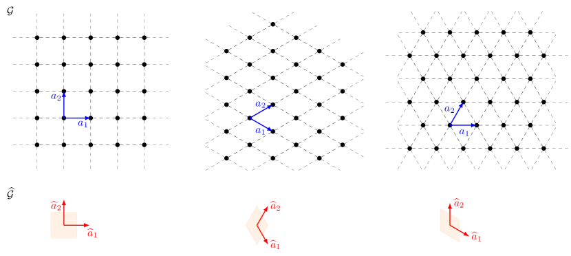
Example 2.1.
If we choose the canonical basis vectors , we have simply
Compare also the left lattice in Figure 1.
In Figure 1 we sketched some Bravais lattices together with their Fourier cells . Note that the dashed lines between the points of the lattice are at this point a purely artistic supplement. However, they will become meaningful later on: If we imagine a particle performing a random walk on the lattice , then the dashed lines could be interpreted as the jumps it is allowed to undertake. From this point of view the lines will be drawn by the diffusion operators we introduce in Section 3.
Definition 2.2.
Given a Bravais lattice as defined in (2) we write
for the sequence of Bravais lattice we obtain by dyadic rescaling with . Whenever we say a statement (or an estimate) holds for we mean that it holds (uniformly) for all .
Remark 2.3.
The restriction to dyadic lattices fits well with the use of Littlewood-Paley theory which is traditionally built from dyadic decompositions. However, it turns out that we do not lose much generality by this. Indeed, all the estimates below will hold uniformly as soon as we know that the scale of our lattice is contained in some interval . Therefore it is sufficient to group the members of any positive null-sequence in dyadic intervals to deduce the general statement.
Given we define its Fourier transform as
| (4) |
where we introduced a “normalization constant” that ensures that we obtain the usual Fourier transform on as tends to 0. We will also write for the Lebesgue measure of the Fourier cell .
If we consider as a map on , then it is periodic under translations in . By the dominated convergence theorem is continuous, so since is compact it is in , where denotes integration with respect to the Lebesgue measure. For any we define its inverse Fourier transform as
| (5) |
Note that and therefore we get at least for with finite support . The Schwartz functions on are
and we have (with periodic boundary conditions) for all , because for any multi-index the dominated convergence theorem gives
By the same argument we have for all , and as in the classical case one can show that is an isomorphism from to with inverse . Many relations known from the -case carry over readily to Bravais lattices, e.g. Parseval’s identity
| (6) |
(to see this check for example with the Stone-Weierstrass theorem that forms an orthonormal basis of ) and the relation between convolution and multiplication
| (7) | ||||
| (8) |
where is for the unique element in such that .
Since consists of functions decaying faster than any polynomial, the Schwartz distributions on are the functions that grow at most polynomially,
and is well defined for . We extend the Fourier transform to by setting
where denotes the complex conjugate. This should be read as , which however does not make any sense because for we did not define the Fourier transform but only . The Fourier transform agrees with in case . It is possible to show that , where
for , and that is an isomorphism from to with inverse
| (9) |
As in the classical case it is easy to see that we can identify every with a “Dirac comb” distribution by setting
| (10) |
where denotes a shifted Dirac delta distribution. We can identify any element of the frequency space with an -periodic distribution by setting
| (11) |
If coincides with a function on one sees that
| (12) |
where is, as above, the (unique) element such that . Conversely, every -periodic distribution can be seen as a restricted element , e.g. by considering
| (13) |
where is chosen such that and where we used in the second equality the definition of the product between a smooth function and a distribution. To construct such a it suffices to convolve with a smooth, compactly supported mollifier, and it is easy to check that for all and that does not depend on the choice of . This motivates our definition of the extension operator below in Lemma 2.6.
With these identifications in mind we can interpret the concepts introduced above as a sub-theory of the classical Fourier analysis of tempered distributions. We will sometimes use the following identity for
| (14) |
which is easily checked using the definitions above.
Next, we want to introduce Besov spaces on . Recall that one way of constructing Besov spaces on is by making use of a dyadic partition of unity.
Definition 2.4.
A dyadic partition of unity is a family of nonnegative radial functions such that
-
•
is contained in a ball around 0, is contained in an annulus around 0 for ,
-
•
for ,
-
•
for any ,
-
•
If we have ,
Using such a dyadic partition as a family of Fourier multipliers leads to the Littlewood-Paley blocks of a distribution ,
Each of these blocks is a smooth function and it represents a “spectral chunk” of the distribution. By choice of the we have in , and measuring the explosion/decay of the Littlewood-Paley blocks gives rise to the Besov spaces
| (15) |
In our case all the information about the Fourier transform of , that is , is stored in a finite bandwidth . Therefore, it is more natural to decompose the compact set , so that we consider only finitely many blocks. However, there is a small but delicate problem: We should decompose in a smooth periodic way, but if is such that the support of touches the boundary of , the function will not necessarily be smooth in a periodic sense. We therefore redefine the dyadic partition of unity for as
| (18) |
where . Now we set for
which is now a function defined on . As in the continuous case we will also use the notation .
Of course, for a fixed it may happen that , but if we rescale the lattice to , the Fourier cell changes to and so for the following definition becomes meaningful.
Definition 2.5.
Given and we define
where we define the norm by
| (19) |
We write furthermore .
The reader may have noticed that since we only consider finitely many (and since is a bounded operator, uniformly in , as we will see below), the two spaces and are in fact identical with equivalent norms! However, since we are interested in uniform bounds on for , we are of course not allowed to switch between these spaces. Whenever we consider sequences of lattices we construct all dyadic partitions of unity from the same partition of unity on .
With the above constructions at hand it is easy to develop a theory of paracontrolled distributions on a Bravais lattice which is completely analogous to the one on . For the transition from the rescaled lattice models on to models on the Euclidean space we need to compare discrete and continuous distributions, so we should extend the lattice model to a distribution in . One way of doing so is to simply consider the identification with a Dirac comb, already mentioned in (10), but this has the disadvantage that the extension can only be controlled in spaces of quite low regularity because the Dirac delta is quite irregular. We find the following extension convenient:
Lemma 2.6.
Let be a positive function with and set
where the periodic extension is defined as in (11). Then and for all .
Proof.
We have because is in , and therefore also . Knowing that is in , it must be in as well because it has compact spectral support by definition. Moreover, we can write for
where we used the definition of from (11) and that for all and . ∎
It is possible to show that if denotes the extension operator on , then the family is uniformly bounded in , and this can be used to obtain uniform regularity bounds for the extensions of a given family of lattice models.
However, since we are interested in equations with spatially homogeneous noise, we cannot expect the solution to be in for any and instead we have to consider weighted spaces. In the case of the parabolic Anderson model it turns out to be convenient to even allow for subexponential growth of the form for , which means that we have to work on a larger space than , where only polynomial growth is allowed. So before we proceed let us first recall the basics of the so called ultra-distributions on .
2.2 Ultra-distributions on Euclidean space
A drawback of Schwartz’s theory of tempered distributions is the restriction to polynomial growth. As we will see later, it is convenient to allow our solution to have subexponential growth of the form for and . It is therefore necessary to work in a larger space , the space of so called (tempered) ultra-distributions, which has less restrictive growth conditions but on which one still has a Fourier transform. Similar techniques already appear in the context of singular SPDEs in [38], where the authors use Gevrey functions that are characterized by a condition similar to the one in Definition 2.11 below. Here, we will follow a slightly different approach that goes back to Beurling and Björck [3], and which mimics essentially the definition of tempered distribution via Schwartz functions. For a broader introduction to ultra-distributions see for example [45, Chapter 6] or [3].
Let us fix, once and for all, the following weight functions which we will use throughout this article.
Definition 2.7.
We denote by
where For we denote by the set of measurable, strictly positive such that
| (20) |
for some . We also introduce the notation . The objects will be called weights.
Note that the sets are stable under addition and multiplication for a fixed . The indices “” and “” of the elements in indicate the fact that elements in are polynomially growing or decaying while elements in are allowed to have subexponential behavior. Note that
and that
| (21) |
and for . The reason why we only allow for will be explained in Remark 2.10 below.
We are now ready to define the space of ultra-distributions.
Definition 2.8.
We define for the locally convex space
| (22) |
which is equipped with the seminorms
| (23) | |||
| (24) |
Its topological dual is called the space of tempered ultra-distributions.
Remark 2.9.
Remark 2.10.
The reason why we excluded the case for in Definition 2.7 is that we want to contain functions with compact support, which then allows for localization and thus for a Littlewood-Paley theory. But if with and the requirement implies that can be bounded by , , which means that is analytic and the only compactly supported is the zero-function .
In the case the space is strictly larger than . Indeed: for . In the case we simply have
with a topology that can also be generated by only using the seminorms so that the dual of is given by
The theory of “classical” tempered distributions is therefore contained in the framework above.
The role of the triple
in this theory will be substituted by spaces such that
Definition 2.11.
Let be an open set and . We define for the set to be the space of such that for every and compact there exists such that for all
| (25) |
For we set . We also define
| (26) |
The elements of are called ultra-differentiable functions and the elements of the dual space are called ultra-distributions.
Remark 2.12.
The space is equipped with a suitable topology [3, Section 1.6] which we did not specify since this space will not be used in this article and is just mentioned for the sake of completeness.
Remark 2.13.
The relation between and their properties are specified by the following lemma.
Lemma 2.14.
Let .
-
i)
We have and
(27) In particular .
-
ii)
The space is stable under addition, multiplication and convolution.
-
iii)
The space is stable under addition, multiplication and division in the sense that for .
Sketch of the proof.
We only have to prove the statements for . Take and . We then have for
Using further that for (we here follow [31, Lemma 12.7.4])
we obtain for
Choosing big enough shows that satisfies the estimate in (25) (with global bounds) and thus and . In particular we get . To show the inverse inclusion consider . We only have to show that for any and . And indeed for with (without loss of generality)111We here follow ideas from [38, Proposition A.2].
where denote as usual constants that may change from line to line and where in the last step we chose small enough to make the series converge; note that the bound (25) holds on all of because is compactly supported by assumption.
The stability of under addition, multiplication and convolution are quite easy to check, see [3, Proposition 1.8.3].
It is straightforward to check that for using Leibniz’s rule. For the stability under composition see e.g. [40, Proposition 3.1], from which the stability under division can be easily derived. ∎
Many linear operations such as addition or derivation that can be defined on distributions can be translated immediately to the space of ultra-distributions . We see with (26) that should be interpreted as the set of smooth multipliers for ultra-distributions in and in particular for tempered ultra-distributions . The space is small enough to allow for a Fourier transform.
Definition 2.15.
For and we set
By definition of we have that and are isomorphisms on which implies that and are isomorphisms on .
The following lemma proves that the set of compactly supported ultra-differentiable functions is rich enough to localize ultra-distributions, which gets the Littlewood-Paley theory started and allows us to introduce Besov spaces based on ultra-distributions in the next section.
Lemma 2.16 ([3], Theorem 1.3.7.).
Let . For every pair of compact sets there is a such that
2.3 Ultra-distributions on Bravais lattices
For the discrete setup we essentially proceed as in Subsection 2.1 and define spaces
and their duals (when equipped with the natural topology)
with the pairing , . As in Subsection 2.1 we can then define a Fourier transform on which maps the discrete space into the space of ultra-differentiable functions with periodic boundary conditions. The dual space can be equipped with a Fourier transform as in (9) such that become isomorphisms between and that are inverse to each other. For a proof of these statements we refer to Lemma A.1.
2.4 Discrete weighted Besov spaces
We can now give our definition of a discrete, weighted Besov space, where we essentially proceed as in Subsection 2.1 with the only difference that is included in the definition and that the partition of unity , from which is constructed as on page 2.1, must now be chosen in .
Definition 2.17.
Given a Bravais lattice , parameters , and a weight for we define
where the Littlewood-Paley blocks are built from a dyadic partition of unity on constructed from some dyadic partition of unity on as on page 2.1. If we consider a sequence as in Definition 2.2 we take the same to construct for all the partitions on .
We write furthermore and define
i.e. .
Remark 2.18.
When we introduce the weight we have a choice where to put it. Here we set , which is analogous to [45] or [28], but different from [38] who instead take the norm under the measure . For both definitions coincide, but for the weighted space of Mourrat and Weber does not feel the weight at all and it coincides with its unweighted counterpart.
Remark 2.19.
The formulation of this definition for continuous spaces , and is analogous.
We can write the Littlewood-Paley blocks as convolutions (on ):
| (28) |
where
We also introduce the notation
Due to our convention to only consider dyadic scalings we always have the useful property
| (29) |
for a lattice sequence as in Definition 2.2, where
| (30) |
and where are Schwartz functions on with . The functions depend on the lattice used to construct but are independent of . In a way, this is a discrete substitute for the scaling one finds on for (for ) due to the choice of the dyadic partition of unity in Definition 2.4. We prove the identity (29), together with a similar result for , in Lemma 2.25 below. It turns out that (29) is helpful in translating arguments from the continuous theory into our discrete framework. Let us once more stress the fact that is defined on all of , and therefore (28) actually makes sense for all . With the from Lemma 2.25 this “extension” coincides with , where the extension operator is defined as in Lemma 2.24 below.
The following Lemma, a discrete weighted Young inequality, allows us to handle convolutions such as (28).
Lemma 2.20.
Given as in Definition 2.2 and for we have for any with and , for the bound
| (31) |
where the implicit constant is independent of . In particular, and for
| (32) |
where we used in the second estimate that
can be canonically extended to .
Remark 2.21.
Using for this covers in particular the functions via (29).
Proof.
The case follows from the definition of and , so that we only have to show the statement for . And indeed we obtain
where we used that and in the application of Lemma A.2 that for the quotient is uniformly bounded. Inequality (31) can be proved in the same way since it suffices to take the supremum over .
From Lemma 2.20 ( and Remark 2.21) we see in particular that the blocks map the space into itself for any :
| (33) |
where the involved constant is independent of and . This is the discrete analogue of the continuous version
| (34) |
for (which can be proved in essentially the same manner).
As in the continuous case we can state an embedding theorem for discrete Besov spaces. Since it can be shown exactly as its continuous (and unweighted) cousin ([1, Proposition 2.71] or [12, Theorem 4.2.3]) we will not give its proof here.
Lemma 2.22.
Given as in Definition 2.2 for any , and weights with we have the continuous embedding (with norm of the embedding operator independent of )
for . If and the embedding is compact.
For later purposes we also recall the continuous version of this embedding.
Lemma 2.23 ([12], Theorem 4.2.3).
For any , and weights with we have the continuous embedding (with norm independent of )
for . If and the embedding is compact.
The extension operator
Given a Bravais lattice and a dyadic partition of unity on such that , as defined on page 2.1, is strictly greater than we construct a discrete dyadic partition of unity from as on page 2.1.
We choose a symmetric function which we refer to as the smear function and which satisfies the following properties:
-
1.
,
-
2.
on for ,
-
3.
The last property looks slightly technical, but actually only states that the support of is small enough such that it only touches the support of the periodically extended with inside . Using it is not hard to construct a function as above: Indeed choose via Lemma 2.16 some that satisfies property 3 and and set .
The rescaled satisfies the same properties on (remember that by convention we construct the sequence from the same ). This allows us to define an extension operator in the spirit of Lemma 2.6 as
and as in Lemma 2.6 we can show that and .
Using (14) we can give a useful, alternative formulation of
| (35) |
where as in (28) we read the convolution in the second line as a function on using that is defined on . By property 3 of we also have for
| (36) |
Finally, let us study the interplay of with Besov spaces.
Lemma 2.24.
For any and the family of operators
defined above, is uniformly bounded in .
Proof.
We have to estimate for . For we can apply (36) and (35) together with Lemma 2.20 to bound
For only contributes due to the compact support of . By spectral support properties we have
From (34) we know that maps into itself and we thus obtain
where we applied once more (35) and Lemma 2.20 in the second step. ∎
Below, we will often be given some functional on discrete Besov functions taking values in a discrete Besov space (or some space constructed from it) that satisfies a bound of the type
| (37) |
We then say that the estimate (37) has the property (on ) if there is a “continuous version” of and a continuous version of and a sequence of constants such that
| () |
In other words we can pull the operator inside without paying anything in the limit. With the smear function introduced above when can now also give the proof of the announced scaling property (29) of the functions .
Lemma 2.25.
Let be as in Definition 2.2 and let . Let be a partition of unity of as defined on page 2.1 and take and . The extensions
are elements of . Moreover there are , independent of , such that for for and with as in (30)
| (38) | |||
| (39) |
The functions and have support in an annulus .
In particular we have for and .
where for .
Proof.
Denote by the partition of unity on from which the partitions are constructed. Let us recall the following facts about
| (40) | ||||
| (41) |
The second property can be seen by rewriting
Recall further that has support in an annulus around .
To prove the claim we only have to show (38) and (39). For and we use that by construction of out of we have inside
so that due to property 2 and 3 of the smear function and (41) it is enough to take
and for by the scaling property of from (40)
For the construction of a bit more work is required. Recall that by definition of our lattice sequence we took a dyadic scaling which implies in particular
| (42) |
for some fixed . Using once more (41) and relation (42) we can write for
for some symmetric function . As in (12) let us denote for by the unique element of for which . One then easily checks
| (43) |
Applying (12) and (43) we obtain for that the periodic extension
is the scaled version of the smooth, -periodic function (to see that the composition with does not change the smoothness, note that equals on a neighborhood of ). Consequently
so that setting with as in (42) finishes the proof. ∎
3 Discrete diffusion operators
Our aim is to analyze differential equations on Bravais lattice that are in a certain sense semilinear and “parabolic”, i.e. there is a leading order linear difference operator, which here we will always take as the infinitesimal generator of a random walk on our Bravais lattice. In the following we analyze the regularization properties of the corresponding “heat kernel”.
3.1 Definitions
Let us construct a symmetric random walk on a Bravais lattice with mesh size which can reach every point (our construction follows [33]). First we choose a subset of “jump directions” such that and a map . We then take as a rate for the jump from to the value . In other words the generator of the random walk is
| (44) |
which converges (for ) pointwise to as tends to 0. In the case and we obtain the simple random walk with limiting generator . We can reformulate (44) by introducing a signed measure
which allows us to write and . In fact we will also allow the random walk to have infinite range.
Definition 3.1.
We write for if is a finite, signed measure on a Bravais lattice such that
-
•
,
-
•
,
-
•
for any we have , where is the total variation of ,
-
•
for and ,
where denotes the subgroup generated by in . We associate a norm on to which is given by
We also write .
Lemma 3.2.
The function of Definition 3.1 is indeed a norm.
Proof.
The homogeneity is obvious and the triangle inequality follows from Minkowski’s inequality. If we have for all . Since we also have for the linearly independent vectors from (2), which implies . ∎
Given as in Definition 3.1 we can then generalize the formulas we found above.
Definition 3.3.
is nothing but the infinitesimal generator of a random walk with sub-exponential moments (Lemma A.5). By direct computation it can be checked that for and with the extra condition we have the identities and . In general is an elliptic operator with constant coefficients,
where is a symmetric matrix. The ellipticity condition follows from the relation and the equivalence of norms on . In terms of regularity we expect therefore that behaves like the Laplacian when we work on discrete spaces.
Lemma 3.4.
We have for , and
where is as in Definition 2.17, and where the implicit constant is independent of . For we further have
where the action of on should be read as
| (45) |
for , where we used the symmetry of in the second step.
Proof.
We start with the first inequality. With we have by spectral support properties . Via (29) we can read and thus as a smooth function in defined on all of . In this sense we read
| (46) |
as a smooth function on in the following. Since integrates affine functions to zero we can rewrite
Using (20) and the Minkowski inequality on the support of we then obtain
where is as in (20). By definition of and monotonicity of we have
so that we are left with the task of estimating
where we applied (46) and Young’s convolution inequality on . Due to (29) and Lemma 2.20 we can estimate the first factor by so that we obtain the total estimate
and the first estimate follows.
To show the second inequality we proceed essentially the same but use instead , where now really denotes the inverse transform of the partition on all of . We then have , so that
As above we can then either get , by bounding each of the two second derivatives separately, or , by exploiting the difference to introduce the third derivative. We obtain the second estimate by interpolation. ∎
3.2 Semigroup estimates
In Fourier space can be represented by a Fourier multiplier :
for . The multiplier is given by
| (47) |
where we used that is symmetric with and the trigonometric identity . The following lemma shows that is well defined as a multiplier (i.e. ). It is moreover the backbone of the semigroup estimates shown below.
Lemma 3.5.
Let and . The function defined in (47) is an element of and
-
•
if with it satisfies for any ,
-
•
for every compact set with , where is the reciprocal lattice of the unscaled lattice , we have for all .
The implicit constants are independent of .
Proof.
We start by showing if , which implies in particular in that case. The proof that for is again similar but easier and therefore omitted. We study derivatives with first. We have
and for
For higher derivatives we use that which gives (where denotes as usual a changing constant)
for any . Using for we end up with
and our first claim follows by choosing .
It remains to show that on , which is equivalent to on . We start by finding the zeros of which, by periodicity can be reduced to finding all with . But if , then for any , which yields with that we must have for as in (2). But since we have with and as in (3). Consequently
and hence . Since is periodic under translations in the reciprocal lattice , its zero set is thus precisely . By assumption and it remains therefore to verify in an environment of to finish the proof.
Note that there is a finite subset such that and , since only finitely many are needed to generate . We restrict ourselves to :
For small enough we can now bound . The term on the right hand side defines (the square of) a norm by the same arguments as in Lemma 3.2, and since it must be equivalent to the proof is complete. ∎
Using that is stable under composition with functions in we see that for and can thus define the Fourier multiplier
for and , which gives the (weak) solution to the problem , . The regularizing effect of the semigroup is described in the following proposition.
Proposition 3.6.
We have for , and
| (48) | ||||
| (49) |
and for
| (50) |
uniformly on compact intervals . The involved constants are independent of .
Proof.
We show the claim for , the arguments for are similar but easier. Using spectral support properties we can rewrite for
| (51) |
where we set for
Using the smear function from Subsection 2.4 we can rewrite this as an expression that is well-defined for all
where is given as in (12) and where we extended (periodically) to all of by relation (47). Consequently, we can apply Lemma 2.25 to give an expression for the scaled kernel
where we wrote with as in Lemma 2.25. Suppose we already know that for any and the estimate
| (52) |
holds. We then obtain from (51) with the bound
and an application of Lemma 2.20 shows (48) and (49) (for (49) we also need (33)). Note that we cheated a little bit as Lemma 2.20 actually requires which is not true, inspecting however the proof of Lemma 2.20 we see that all we used was a suitable decay behavior which is still given.
We will now show (52). Using Lemma 3.7 below we can reduce this task to the simpler problem of proving the polynomial bound for and
| (53) |
with a constant that does not depend on . To show (53) we assume that . Otherwise we are dealing with the scale and the arguments below can be easily modified. Integration by parts gives
where we used that by (47). Now we have the following estimates for
where we used that (with bounds that can be chosen independently of by definition) and we applied Lemma 3.5 with the assumption (which we need because we only defined for ). Together with Leibniz’s and Faà-di Bruno’s formula and a lengthy but elementary calculation (53) follows, which finishes the proof of (48) and (49).
Lemma 3.7.
Let , and . Suppose for any there is a such that for all , and
It then holds for any and
Proof.
This follows ideas from [38, Proposition A.2]. Without loss of generality we can assume (otherwise we get the required estimate by taking ). Recall that we have , where denotes a constant that changes from line to line and is independent of . Consequently, Stirling’s formula gives
where we used so that and where we chose in the last step. ∎
3.3 Schauder estimates
We will follow here closely [21] and introduce time-weighted parabolic spaces that interplay nicely with the semigroup .
Definition 3.8.
Given , and an increasing family of normed spaces we define the space
and for
where
For a lattice , parameters and a pointwise decreasing map we set
where
Remark 3.9.
As in Remark 2.19 the definition of the continuous version is analogous.
Standard arguments show that if is a sequence of increasing Banach spaces with decreasing norms, all the spaces in the previous definition are in fact complete in their (semi-)norms.
The Schauder estimates for the operator
| (54) |
and the semigroup in the time-weighted setup are summarized in the following lemma, for which we introduce the weights
| (55) | ||||
| (56) |
with and . The parameter should be thought of as time. The notation means therefore that we take the time-dependent weight , while stands for the time-dependent weight .
Lemma 3.10.
Let be as in Definition 2.2, , and . If is such that , then we have uniformly in
| (57) |
and if is such that , also
| (58) |
Proof.
The proof is along the lines of Lemma 6.6 in [21] with the use of the simple estimate
which is similar to an inequality from the proof of Proposition 4.2 in [28] and the reason for the appearance of the term in (58) (the factor 2 comes from parabolic scaling). We need so that the singularity is integrable on . ∎
For the comparison of the parabolic spaces the following lemma will be convenient.
Lemma 3.11.
Let be as in Definition 2.2. For and a pointwise decreasing we have
and for and
All involved constants are independent of .
4 Paracontrolled analysis on Bravais lattices
4.1 Discrete Paracontrolled Calculus
Given two distributions , Bony [4] defines their paraproduct as
which turns out to always be a well-defined expression. However, to make sense of the product it is not sufficient to consider and , we also have to take into account the resonant term [18]
which can in general only be defined under compatible regularity conditions such as , with (see e.g. [1] or [18, Lemma 2.1]). If these conditions are satisfied we decompose . Bony’s construction can easily be adapted to a discrete and weighted setup, where of course we have no problem in making sense of pointwise products but we are interested in uniform estimates.
Definition 4.1.
Let be a Bravais lattice, and . We define the discrete paraproduct
| (59) |
where the discrete Littlewood-Paley blocks are constructed as in Section 2. We also write . The discrete resonant term is given by
| (60) |
If there is no risk for confusion we may drop the index on , , and .
In contrast to the continuous theory is well defined without any further restrictions since it only involves a finite sum. All the estimates that are known from the continuous theory carry over.
Lemma 4.2.
Given as in Definition 2.2, and we have the bounds:
-
(i.)
For any
-
(ii.)
for any ,
-
(iii.)
for any with
where all involved constants only depend on but not on . All estimates have the property () if the regularity on the left hand side is lowered by an arbitrary .
Proof.
Similarly as in the continuous case is spectrally supported on a set of the form , where is an annulus around . Similarly, we have for with that the function is spectrally supported in a set of the form , where is a ball around . We give a proof of these two facts in the appendix (Lemma A.6). Using these two observations the proof of the estimates in (i.)-(iii.) follows along the lines of [18, Lemma 2.1]) (which in turn is taken from [1, Theorem 2.82, Theorem 2.85]).
We are left with the task of proving the property (). We show in Lemma 4.3 below that there is an (independent of and ) such that for
| (61) |
Consequently we can write
where we used (61) and . On the other hand we can write
where we used in the second step that is spectrally supported in a ball of size to drop all with . In total we obtain
Note that the two sums on the right hand side are spectrally supported in an annulus of size . Using Lemma 2.24, the fact (by (34)) and that (due to (35) and Lemma 2.20), with uniform bounds, we can thus estimate
Assume without loss of generality that the right hand side of estimate (i.) is bounded by . We then have using (by Lemma 2.25 and Lemma 2.20) and (by (41) and Young’s inequality) for , both with uniform bounds,
In the last step we used that by definition of . This shows the property () for estimate (i.). If the right hand side of estimate (ii.) is uniformly bounded by we obtain the bound
and the property () for (ii.) follows. Considering case (iii.) assume once more that the right hand side is bounded by 1. We get, by once more applying (61),
where we used in the second line that the spectral support of and of is contained in a ball of size to reduce the sum in the second term to . Using then that the terms on the right hand side are spectrally supported in a ball of size we get for
so that we obtain, using once more and ,
where we chose in the second line small enough so that . ∎
Lemma 4.3.
Proof.
Let us fix so that . From Lemma A.6 and the construction of our discrete partition of unity on page 2.1 we know that the spectral support of and the support of and are contained in a set of the form , where is a ball around . Choose such that for with (if any) we have (note that is independent of since by the dyadic scaling of our lattice). In particular we have , . Choose further so big that we have for the smear function
for (independently of ). Choose a such that and outside . We can then reshape
where we used the support properties above to replace by . Now, note that (using formal notation to clarify the argument)
| (62) |
Since only and contribute we have so that in (62). Using that we can replace and in (62) by (the dyadic partition of unity on from which is constructed as on page 2.1), replace by their periodic extension and extend the integral to so that in total
where we used in the second line that the support of the convolution is once more contained in to drop and that to introduce smear functions in the integral. The claim follows. ∎
The main observation of [18] is that if the regularity condition is not satisfied, then it may still be possible to make sense of as long as can be written as a paraproduct plus a smoother remainder. The main lemma which makes this possible is an estimate for a certain “commutator”. The discrete version of the commutator is defined as
If there is no risk for confusion we may drop the index on .
Lemma 4.4.
([19, Lemma 14]) Given , and with and we have
Further, property () holds for if the regularity on the left hand side is reduced by an arbitrary .
4.2 The Modified Paraproduct
It will be useful to define a lattice version of the modified paraproduct that was introduced in [18] and also used in [21, 10].
Definition 4.5.
Fix a function such that and define
We then set
for where this is well defined. We may drop the index if there is no risk for confusion.
Convention 4.6.
As in [21] we silently identify in with if with .
Once more the translation to the continuous case is analogous. The modified paraproduct allows for similar estimates as in Lemma 4.2.
Lemma 4.7.
We further have an estimate in terms of the parabolic spaces that were introduced in Definition 3.8.
Lemma 4.8.
We have for and , pointwise decreasing in , the estimate
for any and any diffusion operator as in Definition 3.3. This estimate has the property () if the regularity on the left hand side is lowered by an arbitrary .
Proof.
The main advantage of the modified paraproduct on is its commutation property with the heat kernel (or ) which is essential for the Schauder estimates for paracontrolled distributions, compare also Subsection 5.2 below. In the following we state the corresponding results for Bravais lattices.
Lemma 4.9.
For , , , and , with pointwise decreasing, we have for
and
where is a discrete diffusion operator as in Definition 3.3. These estimates have the property () if the regularity on the left hand side is lowered by an arbitrary .
Proof.
Again we can almost follow along the lines of the proof in [21, Lemma 6.5] with the only difference that in the derivation of the second estimate the application of the “product rule” of does not yield a term but a more complex object, namely
| (63) |
where and similarly for . The bound for (63) follows from Lemma 4.7 once we show
| (64) |
for any . Note that due to Lemma 2.25 we can write
where with . With
we get (64) by applying Lemma 2.20. The proof of the property () is as in Lemma 4.2 and it uses Lemma 3.4. ∎
5 Weak universality of PAM on
With the theory from the previous sections at hand we can analyze stochastic models on unbounded lattices using paracontrolled techniques. As an example, we prove the weak universality result for the linear parabolic Anderson model that we discussed in the introduction. For with and bounded second derivative we consider the equation
| (65) |
on , where is a two-dimensional Bravais lattice, is a discrete diffusion operator on the lattice as described in Definition 3.3, induced by with for . The upper index “” indicates that we did not scale the lattice yet. The family consists of independent (not necessarily identically distributed) random variables satisfying for
where is a constant of order which we will fix in equation (69) below. We further assume that for every and the variable has moments of order such that
The lower bound for might seem quite arbitrary at the moment, we will explain this choice in Remark 5.6 below. Note that is of order while its expectation is of order , so we are considering a small shift away from the “critical” expectation .
We are interested in the behavior of (65) for large scales in time and space. Setting and modifies the problem to
| (66) |
where is defined on refining lattices in as in Definition 2.2 and where . The potential is scaled so that it satisfies for
-
•
,
-
•
,
-
•
for some .
We consider as a discrete approximation to white noise in dimension . In particular, we expect to converge in distribution to white noise on , and we will see in Lemma 5.5 below that this is indeed the case. In Theorem 5.13 we show that converges in distribution to the solution of the linear parabolic Anderson model on ,
| (67) |
where is white noise on , is the Dirac delta distribution, “” denotes a renormalization and is the limiting operator from Definition 3.3. The existence and uniqueness of a solution to (67) were first established in [28] (for more regular initial conditions) by using a “partial Cole-Hopf transformation” which turns the equation into a well-posed PDE. Using the continuous versions of the objects defined in the Sections above we can modify the arguments of [18] to give an alternative proof of their result, see Corollary 5.12 below. The limit of (66) only sees and forgets the structure of the non-linearity , so in that sense the linear parabolic Anderson model arises as a universal scaling limit.
Let us illustrate this result with a (far too simple) model: Suppose is of the form and let us first consider the following ordinary differential equation on :
for some . If , then describes the evolution of the concentration of a growing population in a pleasant environment, which however shows some saturation effects represented by the factor in the definition of . For the individuals live in unfavorable conditions, say in competition with a rival species. From this perspective equation (65) describes the dynamics of a population that migrates between diverse habitats. The meaning of our universality result is that if we tune down the random potential and counterbalance the growth of the population with some renormalization (think of a death rate), then from far away we can still observe its growth (or extinction) without feeling any saturation effects.
The analysis of (66) and the study of its convergence are based on the lattice version of paracontrolled distributions that we developed in the previous sections and it will be given in Subsection 5.2 below. In that analysis it will be important to understand the limit of and a certain bilinear functional built from it, and we will also need uniform bounds in suitable Besov spaces for these objects. In the following subsection we discuss this convergence.
5.1 Discrete Wick calculus and convergence of the enhanced noise
We develop here a general machinery for the use of discrete Wick contractions in the renormalization of discrete, singular SPDEs with i.i.d. noise which is completely analogous to the continuous Gaussian setting. Moreover, we build on the techniques of [6] to provide a criterion that identifies the scaling limits of discrete Wick products as multiple Wiener-Itô integrals. Our results are summarized in Lemma 5.1 and Lemma 5.4 below and although the use of these results is illustrated only on the discrete parabolic Anderson model, the approach extends in principle to any discrete formulation of popular singular SPDEs such as the KPZ equation or the models. In order to underline the general applicability of these methods we work in this subsection in a general dimension .
Take a sequence of scaled Bravais lattices in dimension as in Definition 2.2. As a discrete approximation to white noise we take independent (but not necessarily identically distributed) random variables that satisfy
-
•
,
-
•
,
-
•
for some .
Note that the family we defined in the introduction of this Section fits into this framework (with and ).
Let us fix a symmetric , independent of , which is on and outside of and define
Let us point out that the used in the construction of does not depend on and only serves to erase the “zero-modes” of to avoid integrability issues. Note that so that is a time independent solution to the heat equation on driven by . Our first task will be to measure the regularity of the sequences , in terms of the discrete Besov spaces introduced in Subsection 2.4. For that purpose we need to estimate moments of sufficiently high order. For discrete multiple stochastic integrals with respect to the variables , that is for sums with whenever for some it was shown in [10, Proposition 4.3] that all moments can be bounded in terms of the norm of and the corresponding moments of the . However, typically we will have to bound such expressions for more general (which do not vanish on the diagonals) and in that case we first have to arrange our random variable into a finite sum of discrete multiple stochastic integrals, so that then we can apply [10, Proposition 4.3] for each of them. This arrangement can be done in several ways, here we follow [30] and regroup in terms of Wick polynomials.
Given random variables over some index set and we set
as well as . According to Definition 3.1 and Proposition 3.4 of [34], the Wick product can be defined recursively by and
| (68) |
For we also write
By induction one easily sees that this product is commutative. In the case we may write instead
Lemma 5.1 (see also Proposition 4.3 in [10]).
Let be as in Definition 2.2 and let be a discrete approximation to white noise as above, and assume . For define the discrete multiple stochastic integral w.r.t by
It then holds for
Proof.
In the following we identify with an enumeration by so that we can write
where , denotes the symmetrized version of
and where we used the independence of to decompose the Wick product (we did not show this property, but it is not hard to derive it from the definition of we gave above). The independence and the zero mean of the Wick products allow us to see this as a sum of nested martingale transforms so that an iterated application of the Burkholder-Davis-Gundy inequality and Minkowski’s inequality as in [10, Proposition 4.3] gives the desired estimate
where we used the bound which follows from (68) and our assumption on . ∎
As a direct application we can bound the moments of and in Besov spaces. We also need to control the resonant term , for which we introduce the renormalization constant
| (69) |
which is finite for all because is compact and is supported away from . We define a renormalized resonant product by
Remark 5.2.
Since (Lemma 3.5 together with the easy estimate ) we have in dimension 2.
Using Lemma 5.1 we can derive the following bounds.
Lemma 5.3.
Let and be defined on as above with (where is as on page 5.1) and let . For and we have
| (70) |
The implicit constant is independent of .
Proof.
Let us bound the regularity of . Recall that by Lemma 2.22 we have the continuous embedding (with norm uniformly bounded in ) . To show (70) it is therefore sufficient to bound for
By assumption we have and can bound uniformly in (for example by Lemma A.2). It thus suffices to derive a bound for , uniformly in and . Note that by (7) with so that Lemma 5.1, Parseval’s identity (6) and on (from Lemma 3.5) imply
which proves the bound for . The bound for follows from the same arguments or with Lemma 3.4.
Now let us turn to . A short computation shows that
and, by a similar argument as above, it suffices to bound in for . We are therefore left with the task of bounding the -th moment of
which with Lemma 5.1 and Parseval’s identity (6) can be estimated by
where in the last step we used that all considered functions are even. Since unless for or and since , we get
using in the last step. ∎
By the compact embedding result in Lemma 2.23 together with Prohorov’s theorem we see that the sequences , , and have convergent subsequences in distribution – note that while the Hölder space is not separable, all the processes above are supported on the closure of for and , which is a separable subspace and therefore we can indeed apply Prohorov’s theorem. We will see in Lemma 5.5 below that converges to the white noise on . Consequently, the solution to should approach the solution of , i.e.
| (71) |
where is defined as in Definition 3.1. The limit of will turn out to be the distribution
| (72) |
for , where the right hand side denotes the second order Wiener-Itô integral with respect to the Gaussian stochastic measure induced by the white noise , compare [32, Section 7.2]. Note that is not a continuous functional of , so the last convergence is not a trivial consequence of the convergence for . To identify the limit of we could use a diagonal sequence argument that first approximates the bilinear functional by a continuous bilinear functional as in [37, 30, 10]. Here prefer to go another route and instead we follow [6] who provide a general criterion for the convergence of discrete multiple stochastic integrals to multiple Wiener-Itô integrals, and we adapt their results to the Wick product setting of Lemma 5.1.
Lemma 5.4 (see also [6], Theorem 2.3).
Let and be as in Lemma 5.1. For let . We identify with a Bravais lattice in dimensions via the orthogonal sum to define the Fourier transform of . Assume that there exist with for all and such that for all . Then the following convergence holds in distribution
where denotes the Wiener-Itô integral against the Gaussian stochastic measure induced by the white noise on .
Proof.
The proof is contained in the appendix. ∎
The identification of the limits of the extensions of and is then an application of Lemma 5.4.
Lemma 5.5.
Proof.
Recall that the extension operator is constructed from where the smear function is symmetric and satisfies on some ball around 0. Since from Lemma 5.3 we already know that the sequence is tight in , it suffices to prove the convergence after testing against :
and by taking linear combinations and applying Lemma 5.4 we see that it suffices to establish each of the following convergences:
| (73) |
for all . We can even restrict ourselves to those with , which implies and for small enough, which we will assume from now on. Note that implies
| (74) |
since by definition of
To show the convergence of to note that we have from (35)
where we used in the first step that is symmetric and in the last step that by our choice of and . Using Lemma 5.4 and relation (74) the convergence of to follows.
For the limit of we use the following formula, which is derived by the same argument as above:
with . In view of Lemma 5.4 it then suffices to note that
is dominated by a multiple of on due to Lemma 3.5, and it converges to
by the explicit formula for in (47).
We are left with the convergence of the third component. Since and we obtain via the ()-Property of the paraproduct
and similarly one gets . We can therefore show instead
| (75) |
Note that we have the representations
with as above and as in (71). The -Fourier transform of is for , where denotes the periodic extension from (12) for (recall again that ). We can therefore apply Lemma 5.4 since for the function is integrable on and thus we obtain (75).
5.2 Convergence of the lattice model
We are now ready to prove the convergence of announced at the beginning of this section. The key statement will be the a priori estimate in Lemma 5.9. The convergence of to the continuous solution on , constructed in Corollary 5.12, will be proven in Theorem 5.13. We first fix the relevant parameters.
Preliminaries
Throughout this subsection we use the same , , a polynomial weight for some and a time dependent sub-exponential weight . We further fix an arbitrarily large time horizon and require for the parameter in the weight . Then we have for any , which will be used to control a quadratic term that comes from the Taylor expansion of the non-linearity . We take as in the beginning of this section with (see Remark 5.6 below) and construct as in Subsection 5.1. We further fix a parameter
| (76) |
with small enough such that the interval is non-empty, which (as we will discuss in the following remark) is possible since .
Remark 5.6 (Why moments).
Let us sketch where the boundaries of the interval (76) come from. The parameter will measure the regularity of below. The upper boundary, that is , arises due to the fact that we cannot expect to be better than , which has regularity below due to Lemma 5.3. The correction is just the price one pays in the Schauder estimate in Lemma 3.10 for the “weight change”. The lower bound is a criterion for our paracontrolled approach below to work. We increase below the regularity of our solutions, by subtraction of a paraproduct, to . By Lemma 4.2 this allows us to uniformly control products with provided
because . This condition can be reshaped to , explaining the lower bound. The interval (76) can only be non-empty if
Lemma 5.3 forces us to take so that the the right hand side can only be true provided , which is equivalent to
Let us mention the simple facts , and which we will use frequently below.
We will assume that the initial conditions are uniformly bounded in and are chosen such that converges in to some . For it is easily verified that this is indeed the case and the limit is the Dirac delta, .
Recall that we aim at showing that (the extension of) the solution to
| (77) |
converges to the solution of
| (78) |
where is a suitably renormalized product defined in Corollary 5.12 below.
Our solutions will be objects in the parabolic space which does not require continuity at . A priori there is thus no obvious meaning for the Cauchy problems (77), (78) (although of course for (77) we could use the pointwise interpretation). We use the common interpretation of (77, 78) as equations for distributions (compare for example [44, Definition 3.3.4]) by requiring and
in the distributional sense on , where denotes the tensor product between distributions. Since we mostly work with the mild formulation of these equations the distributional interpretation will not play a crucial role. Some care is needed to check that the only distributional solutions are mild solutions, since the distributional Cauchy problem for the heat equation is not uniquely solvable [46]. However, under generous growth conditions for for (compare [14]) there is a unique solution. In our case this fact can be checked by considering the Fourier transform of in space.
A priori estimates
We will work with the following space of paracontrolled distributions.
Definition 5.7 (Paracontrolled distribution for 2d PAM).
We identify a pair
with and introduce a norm
| (79) |
for as above, and , . We denote the corresponding space by . If the norm (79) is bounded for a sequence we say that is paracontrolled by .
Remark 5.8.
In view of Remark 3.9 we can also define a continuous version of the space above.
As in [21] it will be useful to have a common bound on the stochastic data: Let
| (80) |
(compared to Lemma 5.3 we have ). The following a priori estimates will allow us to set up a Picard iteration below.
Lemma 5.9 (A priori estimates).
In the setup above consider and . If we require further that and . Define a map
for with via and , where is the solution to the problem
| (81) |
The map is well defined for and we have the bound
for and some , where and
| (82) |
for some that does not depend on , or .
Remark 5.10.
The complicated formulation of (81) is necessary because when we expand the singular product on the right hand side we get
so to obtain the right renormalization we need to subtract , which is exactly what we get if we Taylor expand the second addend on the right hand side of (81).
If is a fixed point, then and the “renormalization term” is just . Moreover we have in this case
Proof.
We assume for the sake of shorter formulas , the general case can be easily included in the reasoning below. The solution to (81) can be constructed using the Green’s function and Duhamel’s principle. To uncluster the notation a bit, we will drop the upper index on in this proof. We show both estimates at once by denoting by either or .
Throughout the proof we will use the fact that
| (83) |
for all which follows from Lemma 4.8. In particular (with ) we have
| (84) |
This leaves us with the task of estimating . We split
| (85) | ||||
| () | ||||
| () | ||||
| () | ||||
| () | ||||
| () |
where so that with and where . We have by Lemmas 4.2, 4.9
and further with Lemma 4.4 and Lemma 4.2
while the term ( ‣ 5.2) can be bounded with Lemma 4.2 by
To estimate () we use the simple bounds for , , , and
for , , , together with the assumption , and obtain for
for all (which is nonempty if is sufficiently small). Similarly we get for
for all . In total we have
where we used for the initial condition that by Definition 4.5 and Convention 4.6 we have for and for . The Schauder estimates of Lemma 3.10 yield on these grounds
where in the last step we used Lemma 3.11. Together with (84) the claim follows. ∎
As we mentioned in Remark 5.10 we aim at finding fixed points of which is achieved by the following Corollary.
Corollary 5.11.
Proof.
We construct the fixed point by a Picard type iteration. To avoid notational clashes with the initial condition , we start the iteration with for which we define for and for (which is in due to Lemma 3.10). Define recursively for the sequence (with to be read as a pair as in Definition 5.7). Choose now so big that and such that
with as in Lemma 5.9. Note that for the constant in principle depends on , but in fact we can choose it independently of since for all (by definition of ) and (by Definition 4.5 and Convention 4.6) in the second term of (82).
Since we already know for that
| (87) |
We show recursively that (87) is in fact true for any . Suppose we have already shown the statement for , we then obtain by Lemma 5.9
By Lemma A.7 in the appendix inequality (87) implies that for and there is a subsequence , convergent in to some , and
In particular is a fixed point of that satisfies (86). It remains to check uniqueness. Choose two fixed points , which then satisfy
We will use that for and with
| (88) |
which is an easy consequence of Definition 2.17 and which we essentially already used in the proof of Lemma 5.9. In other words, we can consider our objects as arbitrarily “smooth” if we are ready to accept negative powers of . In particular, we can consider the initial condition as paracontrolled, that is (and thus ), so that with Lemma 5.9 we obtain . Consequently, since also , we get which implies that the integral term is in and, by using once more (88), we can consider it as an element of for any . The product can then be estimated as in the proof of Lemma 5.9. Since multiplication by only contributes an (-dependent) factor we obtain for a bound of the form
which shows for small enough. Iterating this argument gives on all of . ∎
Convergence to the continuum
It is straightforward to redo our computations in the continuous linear case (i.e. ), which leads to the existence of a solution to the continuous linear parabolic Anderson model on , a result which was already established in [28]. Since the continuous analogue of our approach is a one-to-one translation of the discrete statements and definitions above from to we do not provide the details.
Corollary 5.12.
Sketch of the proof.
As in Lemma 5.9 we can build a map via
| (90) |
As in Corollary 5.11 there is a time such that has a (unique) fixed point in that solves
on . Since the right hand side of (90) is linear, this time can be chosen of the form , where is a (random) constant that only depends on , but not on the initial condition. Proceeding as above but starting in we can construct a map by (the continuous version of) Lemma 5.9 and Lemma 4.9. The map has again a fixed point on which we call . Starting now in we can construct as the fixed point of on and so on. As in [21, Theorem 6.12]) the sequence of local solutions can be concatenated to a paracontrolled solution on .
To see uniqueness take two solutions in and consider . Using that and one derives as in Lemma 5.9
so that choosing first small enough and then proceeding iteratively yields . ∎
We can now deduce the main theorem of this section. The parameters are as on page 76.
Theorem 5.13.
Let be a uniformly bounded sequence in such that converges to some in . Then there are unique solutions to
| (91) |
on with random times that satisfy . The sequence is uniformly bounded and the extensions converge in distribution in , , to the solution of the linear equation in Corollary 5.12.
Remark 5.14.
Since is a random time for which it might be true that the convergence in distribution has to be defined with some care: We mean by in distribution that for any , we have and further .
Proof.
The local existence of a solution to (91) is provided by Corollary 5.11. Proceeding as in the proof of Corollary 5.12 we can in fact construct a sequence of local solutions on intervals with , where we set and . Due to Corollary 5.11 the time is given by
| (92) |
Note that, in contrast to the proof of Corollary 5.12, now really depends on and we might have . As in [21, Theorem 6.12] we can concatenate the sequence to a solution to (91) which is defined up to its “blow-up” time
(which might be larger than or even infinite). Let us set
| (93) |
To show we prove that for any we have . By inspecting the definition of in the proof of Corollary 5.11 we see that given the (bounded) sequence of initial condition the size of can be controlled by the quantity . More precisely there is a deterministic, decreasing function such that
and such that for any (due to the presence of the factor in (92))
| (94) |
Let and . Note that we must have since otherwise we contradict (94). But this already implies the desired convergence:
where we used in the last step the boundedness of the moments of due to Lemma 5.3.
It remains to show that the extensions converge to . By Skohorod representation we know that in Lemma 5.5 converge almost surely on a suitable probability space. We will work on this space from now on. The application of the Skohorod representation theorem is indeed allowed since the limiting measure of these objects has support in the closure of smooth compactly supported functions and thus in a separable space. We can further assume by Skohorod representation that (a.s.) so that almost surely we have for all with some (random) . Having proved that the sequence is uniformly bounded in we know, by Lemma 2.24, that is uniformly bounded in . Due to (the continuous version of) Lemma A.7 there is at least a subsequence of that converges to some in the topology of . If we can show that this limit solves (89) we can argue by uniqueness that (the full sequence) converges to . We have
| (95) |
where should be read as in (45). Note that the left hand side of (95) converges as
due to Lemma 3.4. For the right hand side of (95) we apply the same decomposition as in (85)=( ‣ 5.2)+( ‣ 5.2)+( ‣ 5.2)+()+(). While (the extensions of) the terms (),() of (85) vanish as tends to , we can use the property () of the operators acting in the terms ( ‣ 5.2), ( ‣ 5.2), ( ‣ 5.2) to identify their limits. Consider for example the product in ( ‣ 5.2) whose extension we can rewrite as
where we applied the property () of (Lemma 4.2) in the second step. By continuity of the involved operators and Lemma 5.5 we thus obtain
Proceeding similarly for all terms in the decomposition of the right hand side of (95) one arrives at
which finishes the proof. ∎
Since the weights we are working with are increasing, the solutions and the limit are actually classical tempered distributions. However, since we need the spaces to handle convolutions in weighted spaces it is natural to allow for solutions in . In the linear case, , we can allow for sub-exponentially growing initial conditions since the only reason for choosing the parameter in the weight smaller than was to be able to estimate to handle the quadratic term. In this case the solution will be a genuine ultra-distribution.
Appendix A Appendix
Results related to Section 2
Lemma A.1.
The mappings defined in Subsection 2.3 map the spaces and to each other.
Proof.
We only consider the non-standard case . Given the sequence
obviously converges to a smooth function that is periodic on . We estimate on (and thus by periodicity uniformly on )
We can use Lemma A.2 for with and of the form ( denoting a positive constant that may change from line to line) which yields
We now proceed as in [31, Lemma 12.7.4] and estimate the integral by the function
Since we can choose arbitrarily large we see that indeed .
For the opposite direction, , we use that by integration by parts for all . With Stirling’s formula and Lemma 3.7 we then obtain . This shows the statement for the pair . The estimates above show that are in fact continuous w.r.t to the corresponding topologies so that the statement for the dual spaces immediately follows. ∎
Lemma A.2.
Given a lattice as in (2) we denote the translations of the closed parallelotope by . Let and set If for a measurable function there exists such that for any there is a with then it also holds
Proof.
Indeed
where we used in that the -dimensional parallelotope has vertices. ∎
Lemma A.3 (Mixed Young inequality).
For and we set for
Then for with
(with the convention ).
Proof.
We assume . The remaining cases are easy to check. The proof is based on Hölder’s inequality on with
Raising this expression to the th power and integrating it shows the claim. ∎
Results related to Section 3
Lemma A.4.
For , , we have uniformly in and
and for
Proof.
With the random walk which is generated by on we can express the semigroup as , so that
An application of the next lemma finishes the proof of the first estimate. The second estimate follows as in Lemma 6.6. of [21]. ∎
Lemma A.5.
The random walk generated by on satisfies for any and
Proof.
We assume , if is of the polynomial form the proof follows by similar, but simpler arguments. In this proof we write shorthand . By the Lévy-Khintchine-formula we have for all . We want to bound first for
To this end we apply Faá-di-Brunos formula with . Note that with Lemma 3.5 for and
Thus with we get for any
where denotes as usual a generic constant that changes from line to line. With we get
and therefore, using once more Stirling’s formula and ,
where in the last step we chose small enough to make the series converge. ∎
Results related to Section 4
Lemma A.6.
Let as in Definition 2.2, let , and let be a partition of unity as on page 2.1. For the function
is spectrally supported in a set of the form , where is a ball around that can be chosen independently of and . For and the function
is spectrally supported in a set of the form , where is an annulus around that can be chosen independently of and .
Proof.
We can rewrite
where we used formal notation in the last step and as in (8). From this one sees that the spectral support of is contained in
| (96) |
where we recall that is a subset of (the closure of) , while the sum of sets in the parentheses should be read as a subset of . Now, by the dyadic scaling of we have for all
for some , independent of and . Set: and consider first the case . In this case we have
On the other hand, if we are in the regime and take a ball around such that and hence for all (by the dyadic scaling of from Definition 2.2 we have so that we can choose independently of ). Choosing then shows the first part of the claim.
Let us now consider . With we see as above that the spectral support of is contained in
| (97) |
We already know from above that this set is contained in a ball of size so that is enough to show that (97) is bounded away from . Since and are symmetric and disjoint, we have due to the scaling from (40) and (41), which we observed in the proof of Lemma 2.25, that
for some and
| (98) |
for some . Note, that we can choose small enough such that . Indeed, otherwise there are , such that for some . But from one sees that which contradicts . This choice of the parameter can be done independently of due to the dyadic scaling of our lattice (Definition 2.2).
Consequently, there exists such that (to see that is independent of , use once more the dyadic scaling of the sequence ). But then we have
which closes the proof.
∎
Results related to Section 5
Proof of Lemma 5.4.
We will write shorthand and . The claimed convergence is a consequence of the results in [6]. For let , where denote the vectors that span . For let be the (unique) element in such that and for set . We will start by showing
| (99) |
for all .
By Parseval’s identity we have , where denotes the Fourier transform on for which one easily checks that
where we recall that is the periodic extension of the discrete Fourier transform of (on ) as in (12) and where
The function is uniformly bounded and tends to as goes to . Now we apply Parseval’s identity, once on and once on , and obtain
and thus
Since is uniformly in bounded by and since converges pointwise to zero, it follows from the dominated convergence theorem that converges to zero in . Thus, we get
where for the first term we used that is uniformly bounded in and that by assumption converges to in and for the second term we combined the fact that converges pointwise to with the dominated convergence theorem. We have therefore shown (99). Note that this implies
| (100) |
As in the proof of Lemma 5.1 we identify with an enumeration and use the set so that we can write
where we denote as in the proof of Lemma 5.1 by the symmetrized restriction of to . By Theorem 2.3 of [6] we see that due to (100) the term of converges in distribution to the desired limit, so that we only have to show that the remaining terms vanish as tends to 0. The idea is to redefine for fixed the noise as where , so that in view of [6, Lemma 2.3] it suffices to show that
but this follows from (100). ∎
Lemma A.7.
Let be a sequence which is bounded in the space and let and . There is a subsequence , convergent in , with limit such that
| (101) |
Proof.
Take in the following and . By Definition of we know that is bounded in . Interpolation then shows that is bounded in for some . We obtain by compact embedding (Lemma 2.22) for the existence of a convergent subsequence in with some limit . From the convergence of in it follows that for we have in .
The estimate (101) is then just an iterative application of Fatou like arguments for the norms from which is constructed. ∎
Glossary
- (discrete) Dyadic partition unity
- Set of functions that classify weights
References
- [1] H. Bahouri, J.-Y. Chemin, and R. Danchin. Fourier Analysis and Nonlinear Partial Differential Equations. Springer-Verlag, 2011.
- [2] I. Bailleul and F. Bernicot. Heat semigroup and singular PDEs. J. Funct. Anal., 270(9):3344–3452, 2016.
- [3] G. Björck. Linear partial differential operators and generalized distributions. Arkiv för Matematik, 6(4):351–407, 1966.
- [4] J.-M. Bony. Calcul symbolique et propagation des singularites pour les équations aux dérivées partielles non linéaires. (Symbolic calculus and propagation of singularities for nonlinear partial differential equations). Ann. Sci. Éc. Norm. Supér. (4), 14:209–246, 1981.
- [5] Y. Bruned, M. Hairer, and L. Zambotti. Algebraic renormalisation of regularity structures. arXiv preprint arXiv:1610.08468, 2016.
- [6] F. Caravenna, R. Sun, and N. Zygouras. Polynomial chaos and scaling limits of disordered systems. J. Eur. Math. Soc., 19:1–65, 2017.
- [7] R. Catellier and K. Chouk. Paracontrolled Distributions and the 3-dimensional Stochastic Quantization Equation. ArXiv e-prints, October 2013.
- [8] A. Chandra and M. Hairer. An analytic BPHZ theorem for regularity structures. arXiv preprint arXiv:1612.08138, 2016.
- [9] A. Chandra and H. Shen. Moment bounds for SPDEs with non-Gaussian fields and application to the Wong-Zakai problem. Electron. J. Probab., 22, 2017.
- [10] K. Chouk, J. Gairing, and N. Perkowski. An invariance principle for the two-dimensional parabolic Anderson model with small potential. Stoch. Partial Differ. Equ. Anal. Comput., 5(4):520–558, 2017.
- [11] A. Debussche and G. Da Prato. Strong solutions to the stochastic quantization equations. The Annals of Probability, 31, 2003.
- [12] D.E. Edmunds and H. Triebel. Function Spaces, Entropy Numbers, Differential Operators. Cambridge Tracts in Mathematics. Cambridge University Press, 1996.
- [13] D. Erhard and M. Hairer. Discretisation of regularity structures. arXiv preprint arXiv:1705.02836, 2017.
- [14] A. Friedman. Partial differential equations of parabolic type. Prentice-Hall, 1964.
- [15] P. Friz and N. Victoir. Differential equations driven by Gaussian signals. Ann. Inst. Henri Poincaré Probab. Stat., 46(2):369–413, 2010.
- [16] P. Gonçalves and M. Jara. Nonlinear fluctuations of weakly asymmetric interacting particle systems. Arch. Ration. Mech. Anal., 212(2):597–644, 2014.
- [17] M. Gubinelli, H. Koch, and T. Oh. Renormalization of the two-dimensional stochastic nonlinear wave equation. ArXiv e-prints, March 2017.
- [18] M. Gubinelli, P. Imkeller, and N. Perkowski. Paracontrolled distributions and singular PDEs. Forum of Mathematics, Pi, 3, 2015.
- [19] M. Gubinelli and N. Perkowski. Lectures on singular stochastic PDEs. Ensaios Mat., 29, 2015.
- [20] M. Gubinelli and N. Perkowski. The Hairer-Quastel universality result at stationarity. RIMS Kokyuroku Bessatsu, B59, 2016.
- [21] M. Gubinelli and N. Perkowski. KPZ reloaded. Comm. Math. Phys., 349(1):165–269, 2017.
- [22] M. Gubinelli and N. Perkowski. Energy solutions of KPZ are unique. J. Amer. Math. Soc., 31(2):427–471, 2018.
- [23] M. Hairer and K. Matetski. Discretisations of rough stochastic PDEs. Ann. Probab., 46(3):1651–1709, 2018.
- [24] M. Hairer and J. Quastel. A class of growth models rescaling to KPZ. ArXiv e-prints, December 2015.
- [25] M. Hairer and W. Xu. Large scale behaviour of 3D continuous phase coexistence models. ArXiv e-prints, January 2016.
- [26] M. Hairer. Solving the KPZ equation. Ann. Math. (2), 178(2):559–664, 2013.
- [27] M. Hairer. A theory of regularity structures. Invent. Math., 198(2):269–504, 2014.
- [28] M. Hairer and C. Labbé. A simple construction of the continuum parabolic anderson model on . Electron. Commun. Probab., 20:11 pp., 2015.
- [29] M. Hairer and J. Maas. A spatial version of the Itô-Stratonovich correction. Ann. Probab., 40(4):1675–1714, 2012.
- [30] M. Hairer and Hao Shen. A central limit theorem for the KPZ equation. Ann. Probab., 45(6B):4167–4221, 2017.
- [31] L. Hörmander. The Analysis of Linear Partial Differential Operators II. Springer Berlin Heidelberg, 2005.
- [32] S. Janson. Gaussian Hilbert spaces, volume 129 of Cambridge Tracts in Mathematics. Cambridge University Press, Cambridge, 1997.
- [33] F. Lawler and V. Limic. Random Walk: A Modern Introduction. Cambridge University Press, 2010.
- [34] J. Lukkarinen and M. Marcozzi. Wick polynomials and time-evolution of cumulants. J. Math. Phys., 57(8):083301, 27, 2016.
- [35] T. Lyons. Differential equations driven by rough signals. Rev. Mat. Iberoamericana, 14, 1998.
- [36] K. Matetski, J. Quastel, and D. Remenik. The KPZ fixed point. arXiv preprint arXiv:1701.00018, 2016.
- [37] J.-C. Mourrat and H. Weber. Convergence of the two-dimensional dynamic Ising-Kac model to . Comm. Pure Appl. Math., 70(4):717–812, 2017.
- [38] J.-C. Mourrat and H. Weber. Global well-posedness of the dynamic model in the plane. Ann. Probab., 45(4):2398–2476, 2017.
- [39] T. Oh and L. Thomann. Invariant Gibbs measures for the 2-d defocusing nonlinear wave equations. arXiv preprint arXiv:1703.10452, 2017.
- [40] A. Rainer and G. Schindl. Composition in ultradifferentiable classes. ArXiv e-prints, October 2012.
- [41] L. Rodino. Linear partial differential operators in Gevrey spaces. World Scientific, 1993.
- [42] H. Shen and H. Weber. Glauber dynamics of 2D Kac-Blume-Capel model and their stochastic PDE limits. J. Funct. Anal., 275(6):1321–1367, 2018.
- [43] H. Shen and W. Xu. Weak universality of dynamical : non-Gaussian noise. Stoch. Partial Differ. Equ. Anal. Comput., 6(2):211–254, 2018.
- [44] H. Triebel. Higher Analysis. Hochschulbücher für Mathematik. Barth, Heidelberg, 1992.
- [45] H. Triebel. Theory of Function Spaces. Modern Birkhäuser Classics. Springer Basel, 1983.
- [46] A. Tychonoff. Théoremes d’unicité pour l’équation de la chaleur. Rec. Math. Moscou, 42:199–215, 1935.
- [47] R. Zhu and X. Zhu. Lattice approximation to the dynamical model. Ann. Probab., 46(1):397–455, 2018.