Vertical Bifacial Solar Farms: Physics, Design, and Global Optimization

Abstract

There have been sustained interest in bifacial solar cell technology since 1980s, with prospects of 30-50% increase in the output power from a stand-alone single panel. Moreover, a vertical bifacial panel reduces dust accumulation and provides two output peaks during the day, with the second peak aligned to the peak electricity demand. Recent commercialization and anticipated growth of bifacial panel market have encouraged a closer scrutiny of the integrated power-output and economic viability of bifacial solar farms, where mutual shading will erode some of the anticipated energy gain associated with an isolated, single panel. Towards that goal, in this paper we focus on geography-specific optimizations of ground-mounted vertical bifacial solar farms for the entire world. For local irradiance, we combine the measured meteorological data with the clear-sky model. In addition, we consider the detailed effects of direct, diffuse, and albedo light. We assume the panel is configured into sub-strings with bypass-diodes. Based on calculated light collection and panel output, we analyze the optimum farm design for maximum yearly output at any given location in the world. Our results predict that, regardless of the geographical location, a vertical bifacial farm will yield 10-20% more energy than a traditional monofacial farm for a practical row-spacing of 2m (1.2m high panels). With the prospect of additional 5-20% energy gain from reduced soiling and tilt optimization, bifacial solar farm do offer a viable technology option for large-scale solar energy generation.

1 Introduction

A conventional monofacial panel collects light only from the front side; the opaque back-sheet prevents collection of light scattered from ground (or surroundings) onto the back face of these panels. This extra energy from albedo can be partially recovered using a bifacial panel, where both faces of the panel and the cells are optically transparent. The concept of bifacial panels have been analyzed and experimentally demonstrated since 1980s [1, 2]. Indeed, an isolated bifacial panel has been shown to have up to 50% extra output [2] compared to a monofacial panel. Moreover, recent improvements in the design and fabrication of bifacial cell technology suggest several additional advantages [3]. For example, bifacial cells have a lower operating temperature (absence of infrared absorption at back metal) and better temperature coefficient (e.g., HIT cells)—which would improve lifetime and integrated power output.

Several studies in the literature have reported energy output of isolated, standalone bifacial panels both numerically [4, 5, 6, 7] and experimentally [8, 9, 10]. These studies include optimization of the tilt angle and elevation from ground for a single bifacial panel at various locations in the world. The recent work by Guo et al. [11] provides a global analysis of vertical bifacial panel. Given an albedo threshold, they have shown that an isolated vertical panel will always produce more power compared to an optimally tilted monofacial panel, irrespective of the geographic location.

The energy gain of an isolated panel defines the upper limit of the performance potential of a solar cell technology. Eventually, the panels will have to be installed in a farm, where one must account for the mutual shading of the panels. Clearly, the area-averaged power output will now be reduced. Under these circumstances, it is not clear if the advantages found for isolated panels can still sustain. Recently, Appelbaum [12] has provided a partial answer by analyzing a solar farm at Tel-Aviv (latitude $32^{\circ}$N). His work focused on vertically vs. optimally tilted bifacial panel arrays. The optimally tilted farm yields 32% more energy than the vertical farm (in latitude $32^{\circ}$N)—however, it is not clear how the outputs compare to the monofacial panel array. It is also difficult to know if the conclusions apply to other regions of the world. An analysis that broadens the previous work to all the locations of the world (a global optimization) will be helpful. This analysis is particularly important because ITRPV roadmap projects that the bifacial market share will increase from 5% in 2016 to 30% in 2026 [13]. Many PV manufacturers (e.g., Panasonic, Prism Solar, LG, SolarWorld, Centrotherm, etc.) are now producing bifacial panels. A few recent solar farms (e.g., Asahikawa Hokuto Solar Power Plant in Japan, and La Silla PV plant in Chile) are utilizing bifacial panels. Given this rapid progress, it is important to clearly understand the complex physics, design, and optimization of bifacial solar farms.

Among various farm configurations, vertically aligned bifacial panels have been of particular interest because of reduced soiling (dirt or snow) which increases overall energy output. In addition, the higher output in the afternoon due to the ‘double-humped’ daily output profile [11] coincide with the peak electricity demand. Since optimally tilted bifacial panels will always produce slightly more energy compared to the vertical farms, the analysis of vertically aligned panels may be viewed as a lower limit of energy produced by an optimized bifacial farm.

In this paper, we offer detailed model, physics, and a worldwide perspective regarding ground-mounted vertical bifacial solar farms.

We combine the global meteorological data from NASA with the clear-sky model from Sandia to estimate hourly insolation. This new algorithm bypasses the loading of extremely large hourly database, and allows efficient computation towards global analysis of new technologies while maintaining realistic and daily averaged meteorological information.

Next, we model the direct and diffused light collection [14, 15, 16], as well as the non-trivial physics of albedo light collection [17, 7] while accounting for relevant shadings on the panels and the ground. Our generalized formulation models the non-uniform illumination along the panel height. Only a fraction of the light incident on the panels will produce electricity [18] because of the spatially non-uniform illumination and the nature of the electrical connection for the panels. The second aspect is often not accounted for in literature. We use the spatially non-uniform light collection data along with the appropriate circuit model of the panels to accurately find the hourly energy-output from the panels and the farm.

Mutual shading between adjacent panels penalizes energy-output, thereby restricting panels from being closely packed in the farm. We explain how this results in an optimum period between the panels. At high latitudes, the sun-path is more tilted, resulting in larger optimum panel-period. In addition, at the same latitude, locations with more diffuse insolation tend to have a larger panel-period.

Finally, we present a global perspective on the annual yield of vertical bifacial solar farms. The key conclusion of the paper is this: With inter-row separation of 2m (typically required for maintenance) for 1.2m wide panels, a ground-mounted vertical bifacial farm outperforms a traditional monofacial farm by 10-20%, regardless of the geographical location. The gain may persist even for smaller inter-row separation, once the energy loss due to soiling [19, 20, 21, 22] is accounted for. The performance gain requires a denser packing of vertical bifacial panels, the implication of which must be accounted for in the levelized cost of electricity (LCOE) calculation [23, 24].

In sections 2.1 and 2.2, we present the details of the irradiance model, and the physical model to calculate the light collection and power generation of the panels and the farm. In sections 3.1-3.3, we discuss the physics and design-optimization of the farm. Finally, in section 3.4, we present the global perspective and prospects of the optimally designed vertical bifacial solar farm. Our conclusions are summarized in section 4.

2 Method

2.1 Irradiance model

2.1.1 Simulation of hourly GHI. Temporal solar irradiance data consist of the position of the sun and its intensity. This information is crucial to simulate and optimize the energy yield of solar farms.

To simulate such data, we first start by calculating the position of the sun (solar Zenith $\theta_{Z}$ and Azimuth $\gamma_{S}$ angles) at arbitrary time and geographic locations by using the NREL’s solar position algorithm [25] implemented in Sandia model library [26]. Here, $\theta_{Z}$ is the refraction-corrected Zenith angle, which depends on altitude and ambient temperature. Second, we input the sun position data into the Haurwitz clear sky model to generate the Global Horizontal Irradiance (GHI or $I_{GHI}$) [27, 28] on a minute-to-minute basis. Note that the clear sky model often overestimates insolation, especially when the atmosphere is cloudy or overcast. Hence, in the third and final step, we integrate the simulated GHI over time, which is then scaled to match the satellite-derived monthly average GHI data (for 22 years) from the NASA Surface meteorology and Solar Energy database [29], whereby local variation of GHI caused by cloudiness and altitude is incorporated into the calculation. Therefore, our modeling framework fully incorporates the impacts of geographic and climatic factors into modeling the solar irradiance.

Figure 1: (a) The zenith and azimuth angles ($\theta_{Z}$, $\gamma_{S}$) of the sun is shown at a specific time. An example of the sun-path is shown by the red line. (b) The vertical bifacial solar farm is depicted with relevant definitions. (c) This shows the angle of incidence (AOI) on the panel at the specific solar position.

2.1.2 Decomposition of GHI into DHI and DNI. Calculating the irradiance on a tilted surface requires decomposing GHI into two components: Direct Normal Irradiance (DNI or $I_{b}$) and Diffuse Horizontal Irradiance (DHI or $I_{diff}$). The relationship between the two components can be written as

$$I_{GHI}=I_{b}\cos\theta_{Z}+I_{diff}.$$ (1)

Based on (1), however, it is impossible to separate $I_{b}$ and $I_{diff}$ from $I_{GHI}$. Therefore, we estimate the diffuse fraction of $I_{GHI}$ using the Orgill and Hollands model which empirically calculate the diffuse fraction using the clearness index of the sky ($k_{T}$) [30]. The clearness index is defined as the ratio between $I_{GHI}$ and extraterrestrial irradiance ($I_{0}$) on a horizontal surface, i.e.,

$$k_{T}=\frac{I_{GHI}}{I_{0}\times\cos\theta_{Z}}.$$ (2)

For a specific time and location, $I_{GHI}$ is already known while the extraterrestrial irradiance can be evaluated analytically [31]; therefore, we can obtain the clearness index $k_{T}$ on a minute-to-minute basis using (2). Knowing $I_{GHI}$ and $k_{T}$, we use the Orgill and Hollands model to determine $I_{diff}$, which allows us to deduce $I_{b}$ from (1). For demonstration, an example calculation of irradiance at Washington DC on September 22 is shown in Fig. 2.

There are several empirical models for decomposing GHI found in literature [32, 33, 34]. Generally, good agreement have been found among these models [35]. Also, we assume isotropic sky model [36] for diffuse irradiance $I_{diff}$. The Perez model [37] provide a more elaborate and somewhat more complex representation of the diffuse light. However, we expect that our numerical results and key conclusion will not be overly sensitive to the model chosen, and the general conclusions will hold irrespective of the assumed models.

2.1.3 Angle of Incidence (AOI) calculation. To evaluate the contribution of the beam component of sunlight (i.e., $I_{b}$), we need to calculate the angle of incidence (AOI) between $I_{b}$ and the front/back surface of vertical bifacial solar panels. It turns out that AOI of an east-west facing vertical bifacial solar panel can be simply expressed as

$$\theta^{(F)} =AOI_{front}=\cos^{-1}\left[\sin\theta_{Z}\times\cos(\gamma_{S}-\pi/2)\right],$$ (3)

$$\theta^{(B)} =AOI_{back}=\cos^{-1}\left[\sin\theta_{Z}\times\cos(\gamma_{S}+\pi/2)\right].$$ (4)

for the front and back surfaces, respectively. In the next section, knowing the angular and irradiance data of sunlight, we will show how to evaluate the optical absorption and power generation of vertically-mounted bifacial solar farms.

2.2 An array collects direct, diffuse, and albedo light

The solar farm consists of vertical bifacial panels of height $h$, separated by a period of $p$, as shown in Fig. 1(b). Each of the panels face E-W and run infinitely along N-S direction. The front face (East facing) sees the sun from sunrise until noon. The back face (West facing) of the panel sees the sun from noon until sunset. In the following, we will first explain light collection by individual panels and we will integrate the contributions from the array to calculate total power output from the farm.

2.2.1 Panel properties: uniform illumination. Let us assume the panels have monofacial-efficiency of $\eta$ for uniform, normal illumination onto the panel. For an angle of incidence (AOI) $\theta$, we can approximate the efficiency as $\eta(\theta)\equiv[1-R(\theta)]\times\eta$. The angle dependent reflectivity of the panel can be empirically written as [38]

$$R(\theta)=1-\frac{1-\exp(-\cos\theta/a_{r})}{1-\exp(-1/a_{r})}.$$ (5)

Here, $a_{r}$ is the angular loss coefficient. In the following calculations, we assume $a_{r}=0.16$, typical for commercial Si solar panels [38].

The efficiency $\eta_{\textit{diff}}$ of the panel under diffuse sunlight (isotropic illumination) will be lower than that under normal (direct) illumination. We assume $\eta=18.9\%$ and $\eta_{\textit{diff}}=15.67\%$ under normal and diffuse illumination on a single face of the panel (estimated using the simulator ‘Tracey’ [39, 40, 41]: see Supplementary Information (SI)). Oblique angles in the diffuse light have higher reflection loss than normal incidence—that is why $\eta_{\textit{diff}}<\eta$.

Experimentally, the cell efficiency observed by illuminating front or the back faces differ by 1-2% [3]. For simplicity, we assume these values to be the same. Our formulation is general, and can be applied for the bifacial efficiency asymmetry by using separate values of $\eta^{(F)}$ and $\eta^{(B)}$ for front and back face efficiencies, respectively.

At any specific time of the day, the two faces of a bifacial panel are illuminated asymmetrically. Therefore, we calculate the power collection from the front and back faces separately. Let us assume that at any given time of the day, AOI for the front and back panel faces are $\theta^{(F)}$ and $\theta^{(B)}$ , respectively. We will focus on the power collection from the front face, and the calculations for the back face will follow a similar approach. We will denote power per unit area of the panel-surface and per unit area of the farm-land by $\widehat{I}_{PV(*)}$ and ${I}_{PV(*)}$, respectively.

2.2.2 Panel properties: non-uniform illumination. During mornings and afternoons, mutual shadowing makes the illumination over the panel spatially non-uniform, with the lower part of the panel receiving less light than the top. For a panel constructed from a set of series connected cells, bypass diodes are placed across different sub-sections of the series-string to avoid reverse breakdown of the shaded cells. We assume $N_{\textit{bypass}}=3$ bypass diodes sub-divide each panel into $N_{\textit{bypass}}=3$ strings. The effect of the shading on lowering the panel output is taken into account based on the analytical approach developed by C. Deline et al. [42]. In this calculation, we assume that the total current is always limited by the bottom string; the validity of the assumption is discussed in the SI-document.

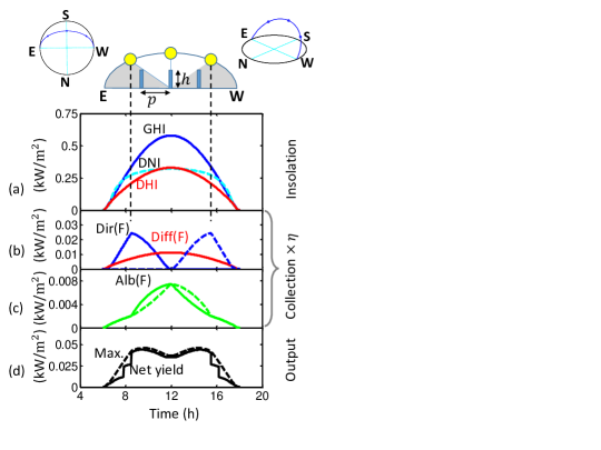
Figure 2: (a) Hourly variation of insolation components for Washington DC on September 22. (b, c, d) The power generation components of the farm is shown. Here, we have assumed $h=1.2$m and $p=2$m.

2.2.3 Direct insolation collection. At any given time of the day, direct illumination component normal to the panel is $I_{b}\cos\theta^{(F)}$ for the unshaded part of the panel (i.e., $z>h_{s}$), see Fig. 6(c). Here, $z$ is any position along the height on the panel, and $h_{s}$ is the shadow on the panel [14, 15] the corresponding time of the day. Considering the reflection loss $R(\theta^{(F)})$ and the panel efficiency $\eta^{(F)}$, we find the power generated per surface area at height $z$ of the front face of the panel as follows,

$$\widehat{I}_{\textit{PV(dir)}}^{(F)}(z)=\begin{cases}[1-R(\theta^{(F)})]\eta^{(F)}I_{b}\cos\theta^{(F)},&z>h_{s}\\ 0,&z\leq h_{s}.\\ \end{cases}$$ (6)

Here, $\widehat{I}_{\textit{PV(dir)}}^{(F)}(z)$ is the power generation component only from the direct/beam sunlight. The corresponding integrated ‘maximum’ power (per unit farm area) from the direct sunlight is given by:

$$I_{\textit{PV(dir),0}}^{(F)} =\frac{1}{p}\times\int_{0}^{h}{\widehat{I}_{\textit{PV(dir)}}^{(F)}(z)\,dz}$$

$$=\frac{(h-h_{s})}{p}[1-R(\theta^{(F)})]\eta^{(F)}I_{b}\cos\theta^{(F)}.$$ (7)

We quote $I_{\textit{PV(dir),0}}^{(F)}$ as the ‘maximum’ output from direct light as this does not assume any loss due to non-uniform generation in the series connected string of cells. This maximum may be reached, for example, in a thin-film like panel configuration. The solid line in Fig. 2(b) shows $I_{\textit{PV(dir),0}}^{(F)}$ as the day progresses. After the solar-noon, the front face will not directly see the sun, therefore $I_{\textit{PV(dir),0}}^{(F)}=0$ for the later part of the day. Similarly, the back face shows a mirrored characteristic for $I_{\textit{PV(dir),0}}^{(B)}$ as shown by the dashed line. These two components together contribute to the characteristic double-humped hourly output profile of a vertical bifacial panel.

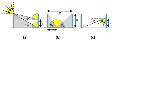
Figure 3: (a) Partial masking of DHI on a face of the panel. (b) Partial masking of DHI on the ground. The fractional DHI reaching the ground is a source for albedo light. (c) Collection of the above mentioned albedo light.

2.2.4 Diffuse insolation collection. Ideally, when the panels are far apart, half of the diffuse rays angle towards the front-face of the panel. These rays cover zenith angle range of $[-\pi/2,0]$. However, a fraction of these angles is obstructed/shaded when the panels are arranged in an array—depicted by the shaded quarter circles in Fig. 3(a). In this illustration, we see that the top portion of the vertical panel receives more diffuse light than the bottom. Calculation of diffuse insolation collection using the well-known average diffuse masking angle [14] will yield in an overestimated value, especially for highly tilted panels. An appropriate view factor [12] properly estimates the diffuse light collection.

The incident diffuse light intensity at height $z$ of the panel (see Fig. 3(a)) is $I_{diff}\times F_{\textit{dz-sky}}$. The diffuse light is masked at angle $\psi(z)$ resulting in the view-factor (towards the unobstructed sky) of $F_{\textit{dz-sky}}=(1-\sin\psi(z))/2$ at $z$ [43]. The corresponding power generation per panel area (front face) from the diffuse insolation is as follows,

$$\widehat{I}_{\textit{PV(diff)}}^{\textit{(F)}}(z) =\eta_{\textit{diff}}^{(F)}\left[I_{\textit{diff}}\times F_{\textit{dz-sky}}\right]$$

$$=\eta_{\textit{diff}}^{(F)}\left[I_{\textit{diff}}\times\frac{1}{2}(1-\sin\psi(z))\right].$$ (8)

And, the corresponding integrated, ‘maximum’ power generation per unit farm area from the diffuse light is:

$$I_{\textit{PV(diff),0}}^{\textit{(F)}} =\frac{1}{p}\times\int_{0}^{h}{\widehat{I}_{\textit{PV(diff)}}^{\textit{(F)}}(z)\,dz}$$

$$=\frac{h}{p}\,\eta_{\textit{diff}}^{(F)}\left[I_{\textit{diff}}\times\frac{1}{2}(1-\tan(\theta_{p}/2))\right].$$ (9)

Here, $\theta_{p}=\tan^{-1}(h/p)$. The hourly variation of $I_{\textit{PV(diff),0}}^{\textit{(F)}}$ is shown by the red solid line in Fig. 2(b). As expected, this component of power generation peaks at noon when the DHI ($I_{diff}$) also peaks. In the above calculations, we can find $\widehat{I}_{\textit{PV(diff)}}^{\textit{(B)}}(z)$ and $I_{\textit{PV(diff),0}}^{\textit{(B)}}$ for the back face by replacing $\eta_{\textit{diff}}^{(F)}$ with $\eta_{\textit{diff}}^{(B)}$.

2.2.5 Albedo light collection. Let us first describe the effect of diffuse insolation on albedo. As explained in the preceding discussion, there is a fractional-shadowing (or masking) of the diffuse light reaching the panel. A similar scenario is true for diffuse light reaching the ground. And, depending on the position between the panels, the amount of diffuse sunlight reaching the ground is different.

Consider a position $x$ between adjacent panels, as in Fig. 3(c). The masking angles from the two panels are:

$$\theta_{1}(x)=\tan^{-1}\frac{h}{x}\quad\mbox{ and, }\theta_{2}(x)=\tan^{-1}\frac{h}{p-x}.$$ (10)

The average masking angles can be written as,

$$\bar{\theta_{1}} =\frac{1}{p}\int_{0}^{p}{\theta_{1}(x)\,dx}=\theta_{p}+\frac{\ln(\csc\theta_{p})}{\cot\theta_{p}}.$$ (11)

Due to symmetry: $\bar{\theta_{1}}=\bar{\theta_{2}}$. Here, $\theta_{p}=\tan^{-1}(h/p)$. The average diffuse insolation reaching the ground is,

$$I_{\textit{Gnd:diff}}=I_{\textit{diff}}\times\frac{1}{2}(\cos\bar{\theta_{1}}+\cos\bar{\theta_{2}})=I_{\textit{diff}}\times\cos\bar{\theta_{1}}.$$ (12)

Note that $\bar{\theta_{1}}$ is constant throughout the day, and $I_{\textit{Gnd:diff}}$ is proportional to $I_{\textit{diff}}$. Diffuse masking on the ground has not been considered in prior literature, although the contribution is particularly important for typical $p/h$. For example, with $p/h\sim 1$, the DHI $I_{\textit{diff}}$ may be masked more than 50% (i.e., $\cos\bar{\theta_{1}}<0.5$). Now, $I_{\textit{Gnd:diff}}\times R_{A}$ can be the diffused light source for the front (or back) face of the panel. The albedo light collection originating from diffuse insolation is masked at angle $\psi_{g}(z)$ at height $z$ on the panel, see Fig. 3(c). Therefore, the corresponding power generation per panel front surface at $z$ is:

$$\widehat{I}_{\textit{PV(Alb:diff)}}^{(F)}(z) =\eta_{\textit{diff}}^{(F)}\,I_{\textit{Gnd:diff}}R_{A}\times F_{\textit{dz-gnd}}$$

$$=\eta_{\textit{diff}}^{(F)}\,I_{\textit{Gnd:diff}}R_{A}\times\frac{1}{2}(1-\sin\psi_{g}(z)).$$ (13)

The corresponding integrated, ‘maximum’ power generation per unit area is given by:

$$I_{\textit{PV(Alb:diff),0}}^{(F)} =\frac{1}{p}\int_{0}^{h}{\widehat{I}_{\textit{PV(Alb:diff)}}^{(F)}(z)\,dz}$$

$$=\frac{h}{p}\,\eta_{\textit{diff}}^{(F)}\,I_{\textit{Gnd:diff}}R_{A}\times\frac{1}{2}\left(1-\tan(\theta_{p}/2)\right).$$ (14)

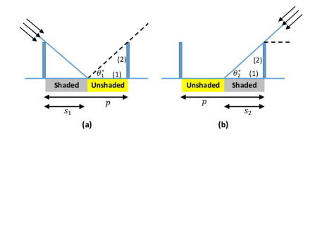
Figure 4: Partial shading of the ground due to DNI during (a) morning, and (b) afternoon.

Next, we can consider albedo from the direct insolation [17]. In the morning, the shading on the ground will be configured as shown in Fig. 4(a). The shade length $s_{1}$ is equal to the period $p$ (i.e., ground fully shaded for the beam component) when the array is turned on. The shade goes away ($s_{1}=0$) at noon. At any time of the day, the unshaded length $(p-s_{1})$ subtends angles $[\psi_{0},\pi/2]$ at the point $z$ on the front panel face (see Fig. 4(a)). In the afternoon, shading $s_{2}$ is adjacent to the front face, Fig. 4(b). In this case, the unshaded region subtends angles $[\psi_{1},\psi_{2}]$ at the point $z$ on the front panel face. We can write:

$$\psi_{0}(z) =\cot^{-1}\left(\frac{p-s_{1}}{z}\right),$$

$$\psi_{1}(z) =\cot^{-1}\left(\frac{p}{z}\right)\mbox{ and }\,\psi_{2}(z)=\cot^{-1}\left(\frac{s_{2}}{z}\right).$$ (15)

The shadow length $s_{1}$ ( or $s_{2}$ ) is calculated for each time-step of the day [14, 15]. Finally, the power generated per area of panel front-face at $z$ from albedo originating from the direct sunlight is calculated as follows:

$$\widehat{I}_{\textit{PV(Alb:dir)}}^{(F)}(z) =\eta_{\textit{diff}}^{(F)}\,I_{\textit{dir}}R_{A}\times F_{\textit{dz-Ugnd}},$$ (16)

where, the view factor from the position $z$ on panel-face to the unshaded part of the ground is given by,

$$F_{\textit{dz-Ugnd}}=\begin{cases}\frac{1}{2}\left(1-\sin\psi_{0}(z)\right),&\mbox{ (before noon)}\\ \frac{1}{2}\left(\sin\psi_{2}(z)-\sin\psi_{1}(z)\right),&\mbox{ (afternoon)}.\\ \end{cases}$$ (17)

And, the corresponding integrated, ‘maximum’ power generated per farm area is:

$$I_{\textit{PV(Alb:dir),0}}^{(F)} =\frac{1}{p}\int_{0}^{h}\widehat{I}_{\textit{PV(Alb:dir)}}^{(F)}(z)\,dz$$

$$=\frac{h}{p}\,\eta_{\textit{diff}}^{(F)}\,I_{\textit{dir}}R_{A}\times F_{\textit{PV-Ugnd}},$$ (18)

where, the view factor from the full panel-face to the unshaded part of the ground is given by,

$$F_{\textit{PV-Ugnd}}=\begin{cases}\frac{1}{2}\left(1-\tan{\frac{\psi_{0}(h)}{2}}\right),&\mbox{ (before noon)}\\ \frac{1}{2}\left(\tan{\frac{\psi_{2}(h)}{2}}-\tan{\frac{\theta_{p}}{2}}\right),&\mbox{ (afternoon)}.\\ \end{cases}$$ (19)

The net ‘maximum’ albedo light contribution from the front-face ($I_{\textit{PV(Alb),0}}^{(F)}=I_{\textit{PV(Alb:dir),0}}^{(F)}+I_{\textit{PV(Alb:diff),0}}^{(F)}$) is shown by the solid line in Fig. 2(c). For the back-face, $I_{\textit{PV(Alb:dir),0}}^{(B)}$ just the flipped version around noon.

Finally, combining Eqs. (7), (9), (14), (18), the ‘maximum’ net power generated per farm area is

$$I_{\textit{PV,0}}^{\textit{(bifacial)}} =\left[I_{\textit{PV(dir),0}}^{\textit{(F)}}+I_{\textit{PV(dir),0}}^{\textit{(B)}}\right]+\left[I_{\textit{PV(diff)}}^{\textit{(F)}}+I_{\textit{PV(diff),0}}^{\textit{(B)}}\right]$$

$$\qquad+\left[I_{\textit{PV(Alb),0}}^{\textit{(F)}}+I_{\textit{PV(Alb),0}}^{\textit{(B)}}\right]$$ (20)

$$=I_{\textit{PV(dir),0}}^{\textit{(bifacial)}}+I_{\textit{PV(diff),0}}^{\textit{(bifacial)}}+I_{\textit{PV(Alb),0}}^{\textit{(bifacial)}}$$ (21)

The black dashed line in Fig. 2(d) shows $I_{\textit{PV,0}}^{\textit{(bifacial)}}$ as the day progresses. Due to partial shading and non-uniform illumination, however, it is not possible to extract this power from the panel configured with the string and bypass-diode connection. A detailed calculation results in the final power generation $I_{\textit{PV}}^{\textit{(bifacial)}}$ per farm area, see black solid line in Fig. 2(d). The abrupt jumps correspond to times when the bypass diodes turns on or off certain sub-strings on the panel. Notice that $I_{\textit{PV}}^{\textit{(bifacial)}}<I_{\textit{PV,0}}^{\textit{(bifacial)}}$ throughout the day. The residual double-humped feature originates from the direct insolation component; otherwise, the power-generation profile is flattened by diffuse and albedo light.

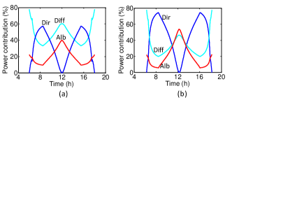
Figure 5: Fractional panel-illumination contribution of direct, diffuse, and albedo light on September 22 in (a) Washington DC, and (b) Jeddah.

3 Results and Discussion

3.1 Hourly energy output

For the following calculations, we assume a typical panel height of $h=1.2$m and the albedo reflectance of 0.5. Albedo reflectance of 0.5 or more is observed naturally for snow-covered ground, or can be achieved artificially for example by white concrete [44].

As discussed earlier, the hourly insolation and power generation from a farm (with period $p=2$m, i.e., $p/h=1.667$) is shown in Fig. 2 for Washington DC (September 22). The fractional contribution of each component (direct, diffuse, and albedo) provides additional information about how the vertical bifacial panel behaves under various weather conditions. For example, in September, the insolation in Washington DC is more diffuse compared to Jeddah. Fig. 5 show the hourly fractional generation from the three components for Washington DC and Jeddah, respectively. We observe that the fractional contribution from diffuse and albedo light peaks at noon. In Washington DC, diffuse and direct components have similar contributions in early part of the day (8-10h). On the other hand, the generation from diffuse light is much lower than direct in early (8-10h) or late (14-16h) part of the day in Jeddah—this indicates that Jeddah has a more clear sky (i.e., mainly direct light). This will affect the net power production at noon. As there is no contribution from direct light at noon, a higher fraction of diffuse light can even out the hourly output variation.

As we will see later, the output varies as a function of the $p/h$-ratio. Therefore, the discussions above hold for any $h$ while $p/h=1.667$ is maintained.

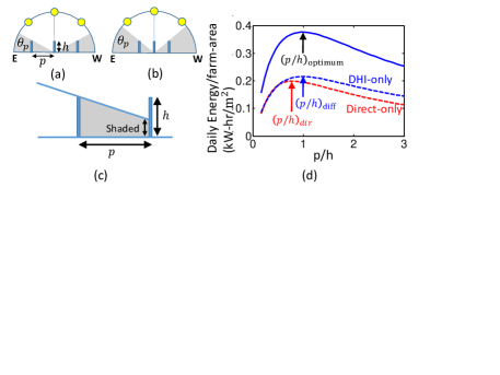
Figure 6: Low elevation of the sun in early morning and late evening causes mutual shading between adjacent panels. The shaded region in (a, b) indicates the time or solar positions when there is mutual shading. Clearly, larger panel-gap $p$ will have shorter shading time as in (a). (c) shows partial shading of a panel for early morning. (d) A single day energy output per farm area is shown (Sept. 22) by the blue solid line. The blue and red dashed line corresponds to the cases when only diffuse sunlight (DHI-only), and only direct sunlight (Direct-only) is considered respectively.

3.2 Effect of panel array period $p$

Next let us consider the effect of the period $p$ on the farm output. Due to the array configuration, front-face of a panel is partially illuminated (partially shadowed) in the early part of the day. For example, in Fig. 6(c), we see the bottom part of the panel is shaded when sun’s elevation is low. In this situation, the bypass diode will turn-off the bottom string of the panel, thereby limiting the output from only the top part of the panel. Similar situation occurs for the back-face of the panel before sunset. The shadow-limited-operating conditions are shown as gray-shaded region in Fig. 6(a, b).

When the panels are packed close (i.e., small $p$), the panels on the farm have bypass-diode limited operation for a long period of each day—this greatly reduces power generation compared to light collection. Again, at large $p$, the output of each panel saturates (to “standalone” panel limit), and thus the farm output per unit area will decrease with increasing $p$. Therefore, there is an optimum $p$ for which the power output per land area is maximized, also shown by the blue solid line in Fig. 6(d). The optimum $p$ scales proportionally with $h$, i.e., universality of the design holds for the $p/h$ ratio. The universality may be understood by realizing that all the expressions for insolation collection contain the ratio $p/h$. For a farm design, instead of integrating over a single day, the output is integrated over the whole year to find a functional relation similar to the one shown in Fig. 6(d) for ‘net annual energy versus $p/h$’. This allows us find maximum annual yield and the corresponding optimum $p/h$ for that specific location. Subsequently, the analysis is repeated for various locations across the globe and a map of the location-specific optimum $p/h$ is shown in Fig. 8(b). The worldwide optimum $p/h$ will be discussed in the next section. It is important to highlight that energy per land area is but one metric of optimization. A levelized cost of electricity (LCOE) optimization will be a part of a future study, but we believe the key conclusion will remain the same.

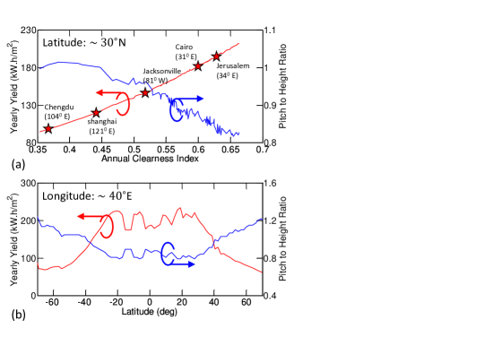
Figure 7: Annual yield and optimum $p/h$ as function of (a) annual clearness index $\bar{k}_{T}$ (latitude $30^{\circ}$N), and (b) latitude (at longitude $40^{\circ}$E).

3.3 Effect of clearness index and latitude.

At a given latitude on Earth, the tilt of the sun and the sun-path is the same for all longitudes. Ideally, we can thus expect the insolation to depend only on latitude. However, variation in meteorological conditions over longitudes at a set latitude causes variation in GHI, clearness index, and the fractional contribution of diffuse insolation. Such variation in weather affects the optimal design of the vertical bifacial solar farm and its yearly yield. For example, in Fig. 7(a) we present the optimum $p/h$ (blue) and the corresponding yearly output (red line) of the farm as a function of annual clearness index $\bar{k}_{T}$ at latitude $30^{\circ}$N—the locations corresponding to the various $\bar{k}_{T}$ are also marked in the figure. Here, we optimize $p/h$ to maximize the annual yield, and calculate the corresponding farm output for different longitudes, but at a fixed latitude $30^{\circ}$N. Then the results are sorted as a function of corresponding $\bar{k}_{T}$ to obtain the plots shown in Fig. 7(a).

At a set latitude, the sun-path is fixed (for all longitude), which in turn determines the panel shadow length and dominates the choice of optimum $p/h$. However, as shown in Fig. 7(a), at a fixed latitude $30^{\circ}$N, there is a small variation in optimal $p/h$ with $\bar{k}_{T}$. In order to understand why $p/h$ decreases with $\bar{k}_{T}$, we need to explain the relative roles of diffuse and direct light. In Fig. 6(d), the blue and red dashed lines consider solar sources when only the diffuse and direct light are present, respectively. For the ‘Direct-only’ case (red dashed line), the diffused light contribution is set to zero and only the direct light and its corresponding albedo contributions are used to calculate the energy output. The output is maximized at $(p/h)_{\textit{dir}}$, as marked by the red arrow. Similarly, for the ‘DHI-only’ case (blue dashed line), the direct sunlight is set to zero, and the diffused light and its albedo contributions are accounted for. The ‘DHI-only’ contribution maximizes at $(p/h)_{\textit{diff}}$, as marked by the blue arrow. In general, for any location, we find that $(p/h)_{\textit{dir}}<(p/h)_{\textit{diff}}$. Therefore, when $\bar{k}_{T}$ is low, DHI or diffuse component dominates and the overall optimum $p/h$ converges to $(p/h)_{\textit{diff}}$. For example, note that the overall peak $(p/h)_{\textit{optimum}}$ (on the blue solid line in Fig. 6(d)) is close to $(p/h)_{\textit{diff}}$ position. Therefore, as shown in Fig. 7(a), reducing $\bar{k}_{T}$ below 0.45 will only keep the $p/h$ at a constant value, close to $(p/h)_{\textit{diff}}$, dictated by the diffuse light component. In contrast, as $\bar{k}_{T}$ increases, the direct light starts to dictate the farm output, and the optimum $p/h$ decreases from $(p/h)_{\textit{diff}}$ and shifts towards $(p/h)_{\textit{dir}}$. Obviously, by definition, increasing $\bar{k}_{T}$ increasing GHI. Therefore, the optimum yearly yield increases with $\bar{k}_{T}$.

The locations with higher latitudes sees larger tilt in the sun-path, and lower GHI. Therefore, the yearly output is high close to the equator and decreases at higher latitudes, as shown by red line in Fig. 7(b). From equator up to latitude $\sim 30^{\circ}$, the optimum $p/h$ remains close to 0.8 (blue line), and then it increases. For higher latitudes, the tilt of the sun (i.e., $\theta_{Z}$) is larger. The longer shadows results in higher spacing between the panels.

3.4 Global Map of Energy Yield

We are now ready to summarize the global optimization and energy yield of vertical bifacial solar farms. We assume a constant ground reflectance of 0.5. As explained earlier, we expect decrease in GHI and output for increasing latitudes. And, there are variation in design and output along the longitudes due to meteorological variations. The global yearly yield and the corresponding optimum $p/h$ is shown in Fig. 8. We observe higher output in Africa and Saudi Arabia compared to India and China due to clearer sky (i.e., higher $\bar{k}_{T}$) and higher GHI. Also, optimum $p/h\sim 0.8$ is close to equator, and begins to increase above $30^{\circ}$ latitude. The optimum $p/h$ is within 0.8-1 for most of the locations in the world.

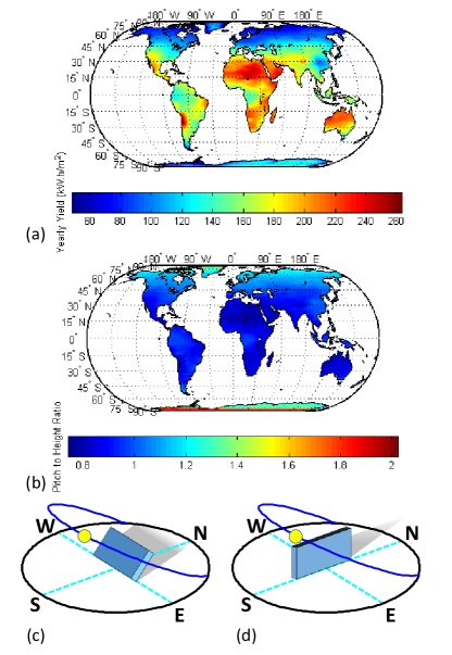
Figure 8: Global optimized (a) yearly yield, and (b) optimum $p/h$ for the vertical bifacial farm. We have chosen constant 50% albedo reflection. The sun-path is shown for latitude $70^{\circ}$N (July) in (c) with South facing monofacial and (d) with East-West facing vertical bifacial panel.

We also compare the vertical bifacial solar farm with the optimized monofacial (optimized tilt [45] and spacing) solar farm. Conventionally, in a monofacial solar farm, the row spacing is selected such that the annual shading loss is less than 5%. This results in a set-back-ratio of 2 closer to equator, and 3 for mid latitudes [45]. For the monofacial farms, we take into account the direct and diffuse insolation, and neglect the albedo. We will compare two cases: when the spacing is optimized for maximum energy yield vs. when the spacing is fixed by practical considerations. Note that the comparison is somewhat biased because while the monofacial farm is tilt-optimized, the vertical farm – by definition – is not.

3.4.1 Spacing optimized solar farms. For the first comparison, we determine the optimum row spacing to maximize the area-normalized annual energy yield of monofacial and bifacial farms for a given location in the world. The ratio of the ‘maximized’ annual yield of the vertical bifacial farm to the monofacial farm is plotted in Fig. 9(a). Close to equator, the monofacial panels are optimally tilted parallel to the ground, and the optimal row spacing is close to zero. Close to equator, therefore, monofacial panels collect the GHI fully, yielding the maximum output for any farm configuration. In these locations, in absence of any soiling considerations, this energy output is twice as large compared to a vertical bifacial farm. The advantage of monofacial farms decreases at higher latitude. At latitudes $>60^{\circ}$, the sun-path is highly tilted. For example, consider the sun-path shown in Fig. 8(c,d) for latitude $70^{\circ}$N in July. The sun is at North-East (or North-West) in early (or late) part of the day. At these times, the South-facing monofacial panel does not receive any direct sunlight (Fig. 8(c)), unlike East-West facing bifacial panel (Fig. 8(d)). Moreover, closer to noon, when the insolation is more significant, we would observe a long shadow towards the North. This result in prominent shading on adjacent South-facing monofacial panels, see Fig. 8(c). The shadows towards the East or West are relatively shorter; therefore, the East-West facing vertical bifacial panels incur lower shading loss. The bifacial panels allows the vertical farm to collect more energy both from the sky and the ground compared to the optimally (and highly) tilted monofacial panel array. In these locations at high latitudes, the bifacial farm produces significantly more energy than monofacial farms.

3.4.2 Spacing with practical considerations. Recall that the period $p$ of an array is defined by the sum of the row spacing and the horizontal distance covered by a tilted panel. Unfortunately, close to equator (within $30^{\circ}$ latitudes), yield-optimized monofacial farms have a row-spacing less than $0.25$m, which is impractically small for installation and maintenance purposes. For example, the row-spacing in the farm is required to be 2m or higher [46]. Therefore, the ‘yield-optimized’ comparison of the farms close to equator (as discussed in the preceding section) may not be practical. Therefore, next we compare the energy yield of the farms with fixed 2m row-spacing.

The ratio of the annual yield of the vertical bifacial farm to the monofacial farm, assuming 2m row-spacing for all, is shown in Fig. 9(b). The conclusion is obvious: For almost all regions of the world, ground-mounted vertical bifacial farms outperform tilt-optimized monofacial farms by 10-20%. Indeed, some regions in Africa and South America may offer 50% more energy output. However, there are a few isolated locations in the world (e.g., parts of China, Columbia, Equador, etc.–marked in deep blue in Fig. 9(b)) where bifacial cell under-performs a monofacial cell by 10-20%. These regions are characterized by low clearness index, so that the shading of the diffuse light at the bottom of the panel and the current-constraint associated with the lower bypass diode strongly penalizes the power output of a bifacial farm (see the corresponding regions in Fig. 8(a)). In these regions, bifacial farms may only be viable if the panels are optimized for tilt angle and energy-penalty due to soiling are accounted for. Indeed, vertical farms seem even more attractive as cleaning costs (e.g., water, labor), etc. are expected to be lower and overall reduction in temperature will improve farm operating lifetime. Therefore, a LCOE-based optimization is essential to accurately quantify the possible gain in utilizing the vertical bifacial farm.

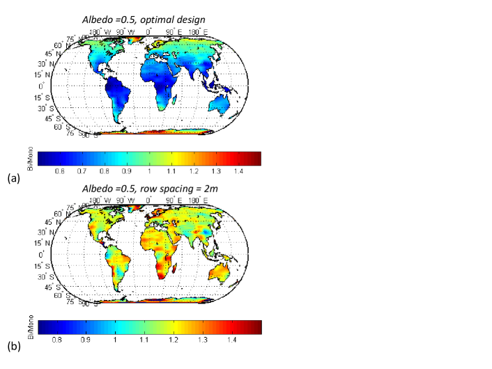
Figure 9: Ratio of yearly yield from the vertical bifacial farm to monofacial farm for (a) optimal design, and (b) fixed row spacing of 2m (1.2m wide panels). In (a), the monofacial farm has optimum panel tilt and row spacing at each location.

4 Summary and Conclusions

In this paper, we have utilized worldwide meteorological data and a detailed physical panel-array model to estimate annual yield of vertical bifacial solar farms. To summarize:

1. We have combined the daily average meteorological NASA data [29] with a clear-sky model from Sandia [26, 27, 28] to obtain hourly insolation information. This combined model greatly reduces loading of large database and speeds up computation while maintaining average meteorological insolation information.

2. Our physics model for panel array combines the effect of direct, diffuse, and albedo illumination onto the panels. The mutual shading and collection from direct and diffuse insolation has been modeled based on previous literature. We have discussed partial shading and illumination onto the ground between panels due to direct and diffuse sunlight. The non-trivial collection of this albedo light has been explained in details. The spatially non-uniform illumination along the panel height can affect the final panel output—our general formulation of the model allows us to calculate such details.

3. Due to non-uniform illumination, and string of series-connected cell configured on a panel, the energy output is not proportional to the insolation collection. We assume that the panel is divided into 3 sub-strings each connected with its own bypass-diodes. The final output of the panels are calculated for this specific configuration.

4. Mutual shading between adjacent panels restricts panels being closely packed in the farm. We explain how this results in an optimum period between the panels. At high latitudes, the sun-path is more tilted, resulting in larger optimum panel-period. And, at the same latitude, locations with more diffuse insolation (i.e., lower $\bar{k}_{T}$) tend to have a larger panel-period.

5. We present a global perspective on the annual yield of vertical bifacial solar farms. For a practical row-spacing of 2m, the energy yield of bifacial solar farms continues to outperform the monofacial solar cells in most of the regions of the world, although the energy gain is somewhat smaller compared to stand-alone panels [11].

Finally, we wish to highlight three factors that will impact the LCOE of a solar farm, but were deemed beyond the scope of the paper. First, the increased energy yield of a bifacial farm requires closely spaced panels. Since the bifacial panels are somewhat more expensive, the LCOE must be calculated carefully to reflect this additional cost. Second, a recent study shows that vertical panels have low dust accumulation while having energy yield similar to conventional tilted panels [47], because of the soiling penalty associated with the monofacial cells. Moreover, cleaning the panels is expensive. Therefore, the energy gain of vertical farms, in practice, may be higher than those summarized in Fig. 9. Finally, a farm designed with optimally tilted and elevated panel array produces much more energy than a ground-mounted vertical bifacial farm [12]. Overall, these energy gains must be balanced carefully with the increased installation cost to ensure the worldwide economic viability of the bifacial solar farms.

References

-
[1]
A. Luque, A. Cuevas, J. Ruiz,
Double-sided
n+-p-n+ solar cell for bifacial concentration, Solar Cells 2 (2) (1980)
151–166.
doi:10.1016/0379-6787(80)90007-1.
URL http://linkinghub.elsevier.com/retrieve/pii/0379678780900071 -
[2]
A. Cuevas, A. Luque, J. Eguren, J. del Alamo,
50
Per cent more output power from an albedo-collecting flat panel using
bifacial solar cells, Solar Energy 29 (5) (1982) 419–420.
doi:10.1016/0038-092X(82)90078-0.
URL http://www.sciencedirect.com/science/article/pii/0038092X82900780 -
[3]
R. Guerrero-Lemus, R. Vega, T. Kim, A. Kimm, L. E. Shephard,
Bifacial
solar photovoltaics – A technology review, Renewable and Sustainable
Energy Reviews 60 (2016) 1533–1549.
doi:10.1016/j.rser.2016.03.041.
URL http://www.sciencedirect.com/science/article/pii/S1364032116002768 -
[4]
A. Luque, E. Lorenzo, G. Sala, S. López-Romero,
Diffusing
reflectors for bifacial photovoltaic panels, Solar Cells 13 (3) (1985)
277–292.
doi:10.1016/0379-6787(85)90021-3.
URL http://linkinghub.elsevier.com/retrieve/pii/0379678785900213 -
[5]
Y. K. Chieng, M. A. Green,
Computer
simulation of enhanced output from bifacial photovoltaic modules, Progress
in Photovoltaics: Research and Applications 1 (4) (1993) 293–299.
doi:10.1002/pip.4670010406.
URL http://onlinelibrary.wiley.com/doi/10.1002/pip.4670010406/abstract - [6] U. Yusufoglu, T. Pletzer, L. Koduvelikulathu, C. Comparotto, R. Kopecek, H. Kurz, Analysis of the Annual Performance of Bifacial Modules and Optimization Methods, IEEE Journal of Photovoltaics 5 (1) (2015) 320–328. doi:10.1109/JPHOTOV.2014.2364406.
-
[7]
J. Appelbaum, View Factors to
Grounds of Photovoltaic Collectors, Journal of Solar Energy
Engineering 138 (6) (2016) 064501–064501–6.
doi:10.1115/1.4034316.
URL http://dx.doi.org/10.1115/1.4034316 -
[8]
G. J. Janssen, B. B. Van Aken, A. J. Carr, A. A. Mewe,
Outdoor
Performance of Bifacial Modules by Measurements and Modelling,
Energy Procedia 77 (2015) 364–373.
doi:10.1016/j.egypro.2015.07.051.
URL http://linkinghub.elsevier.com/retrieve/pii/S187661021500819X - [9] J. E. Castillo-Aguilella, P. S. Hauser, Multi-Variable Bifacial Photovoltaic Module Test Results and Best-Fit Annual Bifacial Energy Yield Model, IEEE Access 4 (2016) 498–506. doi:10.1109/ACCESS.2016.2518399.
-
[10]
M. Lave, J. S. Stein, L. Burnham,
Performance Results for the
Prism Solar Installation at the New Mexico Regional Test
Center: Field Data from February 15 - August 15, 2016, Tech. Rep.
SAND2016-9253, Sandia National Laboratories., Albuquerque, NM (2016).
URL http://energy.sandia.gov/download/38750/ -
[11]
S. Guo, T. M. Walsh, M. Peters,
Vertically
mounted bifacial photovoltaic modules: A global analysis, Energy 61 (2013)
447–454.
doi:10.1016/j.energy.2013.08.040.
URL http://www.sciencedirect.com/science/article/pii/S0360544213007275 -
[12]
J. Appelbaum,
Bifacial
photovoltaic panels field, Renewable Energy 85 (2016) 338–343.
doi:10.1016/j.renene.2015.06.050.
URL http://www.sciencedirect.com/science/article/pii/S0960148115300732 -
[13]
International Technology Roadmap for
Photovoltaic Results 2015, Seventh edition, Tech. rep., ITRPV (Oct.
2016).
URL /Reports/Downloads/2016/ -
[14]
D. Passias, B. Källbäck,
Shading
effects in rows of solar cell panels, Solar Cells 11 (3) (1984) 281–291.
doi:10.1016/0379-6787(84)90017-6.
URL http://www.sciencedirect.com/science/article/pii/0379678784900176 -
[15]
J. Bany, J. Appelbaum,
The
effect of shading on the design of a field of solar collectors, Solar Cells
20 (3) (1987) 201–228.
doi:10.1016/0379-6787(87)90029-9.
URL http://www.sciencedirect.com/science/article/pii/0379678787900299 -
[16]
K. Doubleday, B. Choi, D. Maksimovic, C. Deline, C. Olalla,
Recovery
of inter-row shading losses using differential power-processing submodule
DC–DC converters, Solar Energy 135 (2016) 512–517.
doi:10.1016/j.solener.2016.06.013.
URL http://www.sciencedirect.com/science/article/pii/S0038092X1630192X -
[17]
N. Y. Fathi, A. Samer, View
Factors of Flat Solar Collectors Array in Flat, Inclined, and
Step-Like Solar Fields, Journal of Solar Energy Engineering 138 (6)
(2016) 061005–061005–8.
doi:10.1115/1.4034549.
URL http://dx.doi.org/10.1115/1.4034549 -
[18]
C. R. Sánchez Reinoso, D. H. Milone, R. H. Buitrago,
Simulation
of photovoltaic centrals with dynamic shading, Applied Energy 103 (2013)
278–289.
doi:10.1016/j.apenergy.2012.09.040.
URL http://www.sciencedirect.com/science/article/pii/S0306261912006812 -
[19]
M. J. Adinoyi, S. A. M. Said,
Effect
of dust accumulation on the power outputs of solar photovoltaic modules,
Renewable Energy 60 (2013) 633–636.
doi:10.1016/j.renene.2013.06.014.
URL http://www.sciencedirect.com/science/article/pii/S0960148113003078 -
[20]
N. Bouaouadja, S. Bouzid, M. Hamidouche, C. Bousbaa, M. Madjoubi,
Effects
of sandblasting on the efficiencies of solar panels, Applied Energy 65 (1)
(2000) 99–105.
doi:10.1016/S0306-2619(99)00044-6.
URL http://www.sciencedirect.com/science/article/pii/S0306261999000446 -
[21]
H. Lu, L. Lu, Y. Wang,
Numerical
investigation of dust pollution on a solar photovoltaic (PV) system mounted
on an isolated building, Applied Energy 180 (2016) 27–36.
doi:10.1016/j.apenergy.2016.07.030.
URL http://www.sciencedirect.com/science/article/pii/S0306261916309722 -
[22]
K. Menoufi, Dust Accumulation on
the Surface of Photovoltaic Panels: Introducing the Photovoltaic
Soiling Index (PVSI), Sustainability 9 (6) (2017) 963.
doi:10.3390/su9060963.
URL http://www.mdpi.com/2071-1050/9/6/963 -
[23]
S. A. Janko, M. R. Arnold, N. G. Johnson,
Implications
of high-penetration renewables for ratepayers and utilities in the
residential solar photovoltaic (PV) market, Applied Energy 180 (2016)
37–51.
doi:10.1016/j.apenergy.2016.07.041.
URL http://www.sciencedirect.com/science/article/pii/S0306261916309825 -
[24]
C. S. Lai, M. D. McCulloch,
Levelized
cost of electricity for solar photovoltaic and electrical energy storage,
Applied Energy 190 (2017) 191–203.
doi:10.1016/j.apenergy.2016.12.153.
URL http://www.sciencedirect.com/science/article/pii/S030626191631933X -
[25]
I. Reda, A. Andreas,
Solar
position algorithm for solar radiation applications, Solar Energy 76 (5)
(2004) 577–589.
doi:10.1016/j.solener.2003.12.003.
URL http://www.sciencedirect.com/science/article/pii/S0038092X0300450X -
[26]
PV Performance Modeling Collaborative