Recurrence network measures for hypothesis testing using surrogate data: application to black hole light curves

Abstract

Recurrence networks and the associated statistical measures have become important tools in the analysis of time series data. In this work, we test how effective the recurrence network measures are in analyzing real world data involving two main types of noise, white noise and colored noise. We use two prominent network measures as discriminating statistic for hypothesis testing using surrogate data for a specific null hypothesis that the data is derived from a linear stochastic process. We show that the characteristic path length is especially efficient as a discriminating measure with the conclusions reasonably accurate even with limited number of data points in the time series. We also highlight an additional advantage of the network approach in identifying the dimensionality of the system underlying the time series through a convergence measure derived from the probability distribution of the local clustering coefficients. As examples of real world data, we use the light curves from a prominent black hole system and show that a combined analysis using three primary network measures can provide vital information regarding the nature of temporal variability of light curves from different spectroscopic classes.

1 Introduction

Detecting deterministic nonlinearity in real world data contaminated by different types of noise is a highly nontrivial problem. It is still one of the major challenges in nonlinear time series analysis [1], though several methods and measures have been suggested over the years to address this long standing issue [2, 3]. A generally accepted procedure to detect any nontrivial behavior in a time series is the method of surrogate data [4], for a statistical hypothesis testing, though there are other ways reported in literature to probe nonlinearity of time series without employing surrogates, under certain conditions. Examples are methods related to time-directed network properties of visibility graphs for testing the time-reversal asymmetry [5, 6]. The method of surrogate data involves generating an ensemble of surrogates from the data. A specific null hypothesis is assumed for the data that there is no nontrivial character associated with it. The data and the surrogates are then subjected to the same analysis sensitive to this nonlinear measure. One then tries to statistically reject the null hypothesis for the data by comparing the results for the data and the surrogates [4], with certain confidence level.

In the present analysis, we assume a specific null hypothesis that the data is generated from a linear stochastic process and no nonlinearity is associated with it. We generate a set of surrogate data which are compatible with the null hypothesis of a linear stochastic process. We then use certain measures derived by transforming the time series to a complex network as discriminating measures (as explained below) and try to reject the null hypothesis for the data.

Though the method of surrogate analysis is very popular, there are also many challenges associated with it [7]. For example, generation of proper surrogate data is very important for the success of hypothesis testing. The method to generate surrogate data was initially introduced by Theiler et al. [4] with the Amplitude Adjusted Fourier Transform (AAFT) surrogates. These surrogates are capable of testing the null hypothesis that the data come from linear as well as nonlinear static transformation of a linear stochastic process. An improved version of the AAFT algorithm has been suggested by Schreiber and Schmitz [8, 9] using an iterative scheme called the IAAFT surrogates, which is reported to be more consistent to test null hypothesis [7]. Recently, Nakamura et al. [10] have proposed a surrogate generation method called Truncated Fourier Transform (TFT) [11]. However, the surrogate data generated by this method are influenced by a cut-off frequency. In addition, there are also some other types of surrogate data testing reported in the literature, such as, cycle shuffle surrogates [12], surrogates for testing pseudoperiodic time series [13] and even recurrence based surrogates [14], with each scheme found useful in particular contexts. In this work, we apply the IAAFT scheme to generate surrogate data using the TISEAN package [15].

The second major factor in the surrogate analysis is the choice of a discriminating measure that is sensitive to the nonlinearities associated with the data. In many cases, the correlation dimension $D_{2}$ and the correlation entropy $K_{2}$ have been used as the discriminating measures [16] as they can be directly computed from the time series by the delay embedding method [17]. However, the number of data points should be sufficiently large for a proper computation of these measures. In the paper by Theiler et al. [4], a time reversal asymmetric statistic was introduced which required relatively short time series for computation. In this paper, we consider the use of recurrence network (RN) measures for hypothesis testing, under varying conditions of noise. One obvious advantage of these measures is that they can be computed with reasonable accuracy even when the time series is short (say $<5000$ data points) [18]. Recently, Subramaniyam et al. [18, 19] have used the RN measures for the analysis of EEG data and have shown that these measures can provide insights into the structural properties of EEG in normal and pathological states. Very recently, we have shown that the RN measures can characterize the structural changes in a chaotic attractor contaminated by white and colored noise [20]. Here our aim is to highlight their effectiveness as a tool for hypothesis testing in noisy environment, especially when colored noise is involved. We specifically show that the characteristic path length is very useful in this regard. Moreover, we also present a unique advantage of network based measures for analysis in that the degree distribution as well as the distribution of the local clustering coefficient of the RN provides important information regarding the dimension or the number of variables required to model the underlying system. We specifically derive a convergence factor using the standard Kullback-Leibler measure to identify the dimension beyond which the distributions tend to converge. Details regarding the construction of the RN and the various network measures used in this paper are discussed in the next section.

We use a time series from the Lorenz attractor as prototype to illustrate the effectiveness of using RN measures as discriminating statistic. We add different percentages of white and colored noise to the standard Lorenz attractor time series and the surrogates to get a quantitative estimate of how much noise can swamp the inherent nonlinear behavior and how to fix the threshold of the statistical measure to discriminate between nonlinearity and noise. As examples of real world data involving colored noise, we analyse light curves from the prominent black hole system GRS1915+105. This black hole system is considered to be unique with the light curves falling into $12$ spectroscopic classes [21], whose details are discussed in §4. The system appears to randomly flip in X-ray intensity variations and these observed intensity variations averaged over all energy bands are grouped into $12$ different states. Earlier analysis [22] using the measures $D_{2}$ and $K_{2}$ has strongly indicated deterministic nonlinearity for light curves in $5$ of the $12$ classes. Here we show that analysis using the network measures can provide more exact information regarding the dimensionality of the underlying system as well as the nature of noise contamination in different states.

Finally, it is also important to share some thoughts as to why the proposed method based on RN works. From a conceptual point of view, Donges et al. [23] have shown that all RN properties can be analytically derived from the system’s invariant density. In that case, if we generate IAAFT surrogates from a univariate time series of a nonlinear deterministic system, then by definition, the surrogates will leave the probability distribution invariant. However, the particular phase relationship between different parts of the reconstructed attractor changes. Hence it is important to clarify that the success of the proposed method is based on taking IAAFT surrogates from univariate time series and then use embedding of this surrogate time series, instead of taking the original multivariate time series and their IAAFT surrogates. The latter possibility may result in some distinctly different behavior.

Our paper is organized as follows: In the next section, we discuss the details regarding the construction of the RN and the computation of the network measures to be used for hypothesis testing. In §3, we do surrogate analysis on synthetic data from the Lorenz attractor as well as data obtained by adding different percentages of white and colored noise to the Lorenz data. Analysis of the real world data from the black hole system is presented in §4. Conclusions are drawn in §5.

2 Recurrence networks and related measures

Recurrence is a fundamental property of every dynamical system [24]. This property has been used for developing a two dimensional visualization tool called the recurrence plot (RP) [25]. Considerable information regarding the nature of the underlying dynamical system can be obtained from the RP. To generate the RP, one has to first reconstruct the attractor from the time series using the delay embedding method [17]. The recurrence of trajectory points can then be represented by a two dimensional plot by putting a “dot” at the $\imath,\jmath^{th}$ element if the metric distance between the two points $\imath$ and $\jmath$ on the reconstructed attractor is less than or equal to a threshold value denoted by $\epsilon$. There will obviously be a diagonal line in the RP representing the recurrence of each point with itself. Quantification of the dynamical properties can be obtained from the RP using the so called recurrence quantification analysis [26].

Recently, due to the success of the complex network theory in various fields [27, 28], time series analysis based on the statistical measures of complex networks has also gained a lot of attention. A specific advantage of this approach is that it can be applied to short and nonstationary time series data [29]. For this, the time series is first converted to a complex network defined in an abstract space with a set of nodes $\mathcal{N}={1,2,3,...,N}$ connected by a set of links between the nodes. Several methods have been suggested [30, 31] to transform a time series to a complex network. Here we consider the method of $\epsilon$ - RNs [23, 32] which is based on the property of recurrence of a dynamical system and is closely related to the RP defined above.

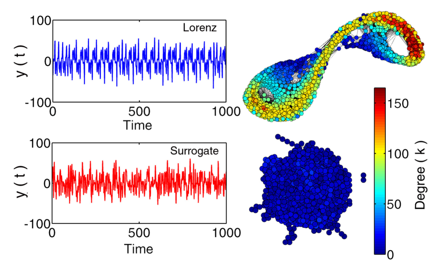
Figure 1: Time series from the standard Lorenz attractor generated from Eq. 4 and the RN constructed from the time series are shown in the top panel. The surrogate time series and the corresponding RN are shown in the bottom panel. Color code represents the variation of the node degree as indicated.

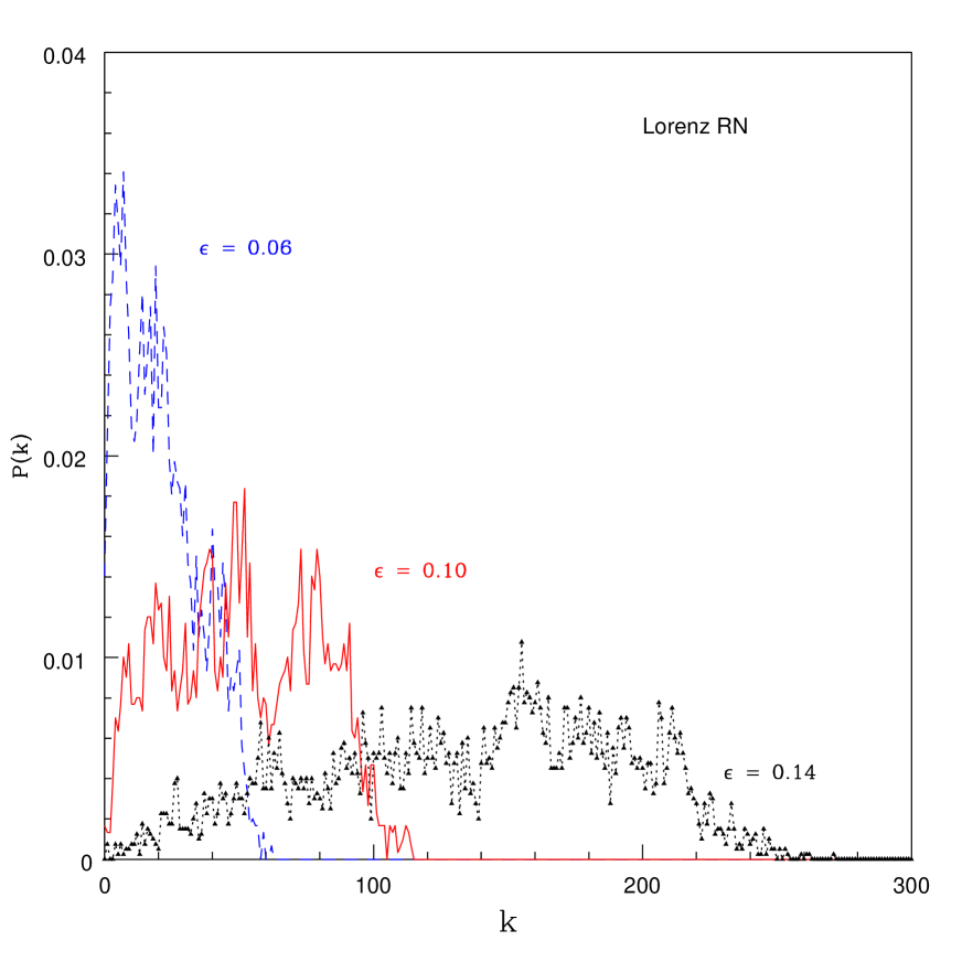
Figure 2: Degree distribution for RNs constructed from the Lorenz attractor using three values of $\epsilon$ as indicated in the figure, with $M=3,N=3000$. The change in the degree distribution is an indicator for selecting the proper value of recurrence threshold (see text).

The attractor is first reconstructed from the given time series using a suitable time delay $\tau$. Here we use the automated algorithmic scheme proposed by us [33] for attractor reconstruction. The scheme involves transforming the time series into a uniform deviate so that the embedded attractor always remains in a unit cube of dimension $M$. The time lag $\tau$ for embedding is chosen as the value of the de-correlation time. A recurrence matrix $\mathcal{R}$ is constructed by a method identical to the construction of the RP. If the distance between two points $\imath$ and $\jmath$ on the attractor is $\leq\epsilon$, the recurrence threshold, the corresponding element on the matrix is $1$ and otherwise $0$. Two nodes $\imath$ and $\jmath$ are considered to be connected only if the corresponding matrix element in $\mathcal{R}$ is $1$. The adjacency matrix $\mathcal{A}$ of the complex network is obtained by removing the self loop (diagonal elements) from the matrix $\mathcal{R}$. It is obvious that the matrix $\mathcal{A}$ is a binary, symmetric matrix implying that the resulting complex network is unweighted and undirected called the RN.

The number of nodes connected to a reference node is called its degree denoted by $k$ and if $N$ is the total number of nodes, $k/N$ is called the degree density. Note that any node in the RN is connected to nodes in its neighbourhood only since the range of connection cannot exceed the threshold value $\epsilon$. In other words, only short range connections exist in a RN. Due to this, the probability density variations over the attractor is mapped onto the local degree density variations over the network as the attractor is transformed into a complex network. Consequently, the node structure of the complex network closely follows the invariant density of the embedded attractor [34]. On the other hand, the topology of the network is reflected in the degree distribution denoted by $P(k)$ which is a probability distribution representing how many nodes have a given degree $k$.

Though the method of transforming the time series to a complex network outlined above is simple and straight forward, care must be taken to ensure that the resulting RN can characterize the properties of the embedded attractor. This is achieved by the proper choice of the recurrence threshold $\epsilon$ and the embedding dimension $M$. We have recently shown [35] that the value of $\epsilon$ is closely related to the choice of $M$. We have also proposed a general method for the construction of RN from a time series, which we follow here. The basic criterion that we use to select the recurrence threshold $\epsilon$ is that the resulting RN should have a giant component and the $\epsilon$ value obtained using this criterion is approximately the same for different time series for a given $M$, due to the uniform deviate transformation. For $M=3$, the value of $\epsilon$ obtained is $0.1$. As an illustrative example, we show in Fig. 1, the time series from the standard Lorenz attractor and its RN (constructed with $M=3$ and $\epsilon=0.1$) along with a surrogate of the time series and the corresponding RN. We use the $y$ - component of the Lorenz system to generate the time series with a time step of $0.05$.

Apart from the presence of the giant component, another method to choose the value of $\epsilon$ is to look at the degree distribution of the resulting RN. When $\epsilon$ is less than the threshold value, there will be large number of nodes with $k\sim 0$ (unconnected nodes) and the resulting $k$ values in the network will be within a small range, centered around a small average value $<k>$. On the other hand, if $\epsilon$ is much greater than the optimum threshold, the network is over connected which may not be easily identified looking at the network. However, in the degree distribution, $P(k)$ will exhibit small values for a wide range of $k$, which implies that the structure of the attractor has not been properly captured by the RN. This will also make the characteristic path length of the network tending to a much smaller value. In between these two extremes, for a small range of $\epsilon$, the resulting network becomes a proper representation of the attractor. This is shown in Fig. 2 for the Lorenz attractor, where degree distribution for RNs with 3 values of $\epsilon$ are shown, using $M=3$ in all cases.

Once the time series is transformed into a complex network, the structural properties of the reconstructed attractor can be characterized by the statistical measures of the complex network. Though many different statistical measures can be defined for a complex network [36], here we concentrate on two for surrogate analysis: an averaged local measure called the average clustering coefficient (CC) and a global network measure, the characteristic path length (CPL). The first one can be defined through a local clustering index $C_{v}$. For the reference node $v$, its value can be determined by finding how many nodes connected to $v$ are also mutually connected:

$$C_{v}={{\sum_{i,j}A_{vi}A_{ij}A_{jv}}\over{k_{v}(k_{v}-1)}}$$ (1)

where $A_{vi}$ are the elements of the adjacency matrix. The average value of $C_{v}$ is taken as the CC of the whole network:

$$CC={{1}\over{N}}\sum_{v}C_{v}$$ (2)

The CPL is defined through the shortest path length $l_{ij}^{s}$ between any pair of nodes $(\imath,\jmath)$ in the network. It represents the minimum number of nodes to be covered to reach from a reference node $\imath$ to any other node $\jmath$ in the network. To calculate CPL, we first compute $l_{ij}^{s}$ for all the nodes in the network and then the global average is found:

$$CPL={{{1}\over{N}}\sum_{i=1}^{N}({{1}\over{N-1}}\sum_{i\neq j=1}^{N-1}l_{ij}^{s})}$$ (3)

Here we try both CPL and CC as discriminating measures for hypothesis testing as discussed in the next section. Apart from these two, we also use the degree distribution $P(k)$ and the distribution of the local clustering coefficient $P(C_{v})$ to gain information regarding the dimension of the underlying system as explained in the next section.

3 Analysis of synthetic data

We first analyze data from the standard Lorenz attractor whose equations are given by:

$${{dx}\over{dt}} = \sigma(y-x)$$

$${{dy}\over{dt}} = x(r-z)$$

$${{dz}\over{dt}} = xy-bz$$ (4)

with the parameter values $\sigma=10$, $r=28$ and $b=8/3$. As mentioned above, one advantage of using network measures is that they can be effectively computed from a relatively low number of nodes in the network. Specifically, since the number of data points in all the black hole light curves is $\sim 3000$, we use the same number of data points for the Lorenz attractor time series as well. To study the effect of noise, we generate an ensemble of data sets by adding different percentages of white and colored noise to the Lorenz data. The colored noise essentially produces a random fractal curve with power varying as $p(f)\propto 1/f^{s}$, where $s$ can, in practice, vary from $1$ to $2$. However, the two most prominent cases in terms of occurence in real world are $s=1$, called $1/f$ noise (which mimics the Brownian motion) and $s=2$, called the red noise. We have generated both and done the analysis adding to the Lorenz data. While the results for $s=1$ is very close to that of white noise, those for $s=2$ are very different and hence we use this case to represent the colored noise in general with $s$ varying from $1.5$ to $2$. Surrogate analysis is performed with $20$ surrogates for each data generated by the TISEAN package [15].

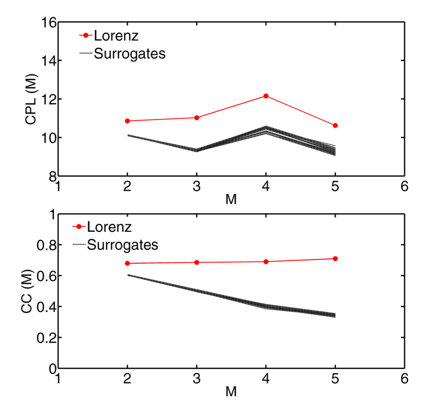
Figure 3: Results of RN analysis of the Lorenz attractor time series with $20$ surrogates using both CPL and CC as quantifying measures. Results for surrogates are shown as dotted black lines. For each $M$, the corresponding value of recurrence threshold $\epsilon$ is used for computing CPL and CC.

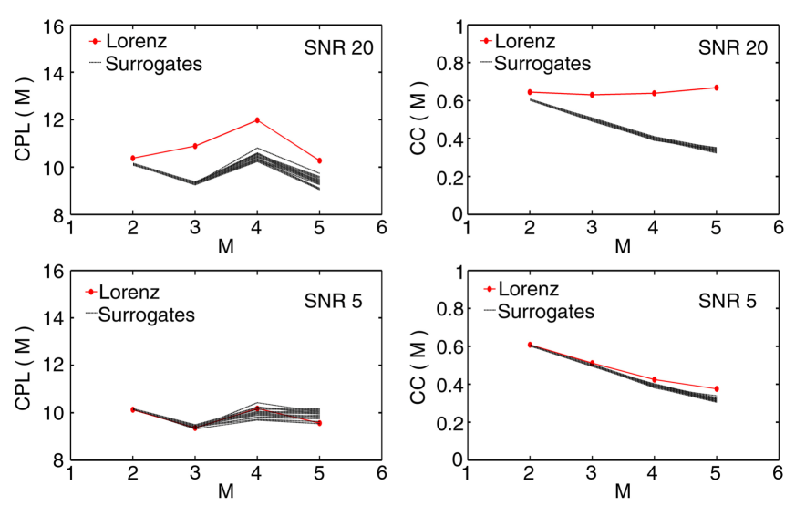
Figure 4: RN analysis of Lorenz data added with two different percentages of white noise and their surrogates with CPL and CC as quantifying measures.

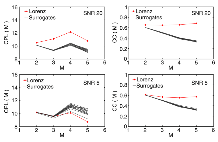
Figure 5: Same as Fig. 4, but with additive red noise instead of white noise.

In Fig. 3, we show the result of RN analysis of the Lorenz attractor time series and its surrogates using both CPL and CC as quantifying measures. For each $M$, we use the value of $\epsilon$ that satisfies the primary criterion of the existence of a giant component in the RN for computing the network measures, as discussed in detail in our scheme [35]. It is clear that the null hypothesis that the data comes from a linear stochastic process can be rejected with high confidence level in both cases. The question may naturally arise why the considered linear surrogates lead to different RN properties than the original data. Though the AAFT surrogates keep the distribution of time series conserved, the nonlinear structures present in the data are destroyed in the surrogates leading to different values of measures after embedding. Effectively, this leads to an altogether different RN compared to that from data, as is evident from Fig. 1.

In order to quantify the results, we use a statistical measure proposed earlier [22], namely, the normalised mean sigma deviation or nmsd. For CC, the measure can be defined as

$$nmsd^{2}={\frac{1}{M_{max}-1}\sum_{M=2}^{M_{max}}\large(\frac{CC(M)-<CC^{surr}(M)>}{\sigma^{surr}_{SD}(M)}\large)^{2}}$$ (5)

with a similar expression for CPL. Here $M_{max}$ is the maximum embedding dimension for which the analysis is undertaken, $CC(M)$ is the CC for the data, $<CC^{surr}(M)>$ is the average CC for $20$ realizations of the surrogate data and $\sigma^{surr}_{SD}(M)$ is the standard deviation of $CC^{surr}(M)$. For the Lorenz time series, $nmsd(CC)=38.46$ and $nmsd(CPL)=26.37$. For pure white noise, the $nmsd$ values are found to be $nmsd(CC)=1.92$ and $nmsd(CPL)=1.64$ while the corresponding values for red noise are obtained as $nmsd(CC)=2.26$ and $nmsd(CPL)=2.08$. The value of $nmsd$ can be used effectively as a quantitative measure to reject the null hypothesis.

The RN analysis of data and surrogates is performed by adding different percentage of white and colored noise to the Lorenz data. The results for two noise levels $5\%$ (SNR $20$) and $20\%$ (SNR $5$) are shown in Fig. 4 for white noise and in Fig. 5 for red noise. From Fig. 4, we find that the data and surrogates become hardly distinguishable when the noise level reaches $20\%$ for both CPL and CC. On the other hand, from Fig. 5 with additive red noise, this is true only for CPL (left panel) and not for CC. Moreover, two other results can also be inferred from these figures:

i) The values of data and surrogates show much deviation beyond the actual dimension of the system.

ii) The CPL of pure data are much above the surrogates. As the noise level increases, the value of the measure for the original data systematically approaches that of the surrogates. However, in some cases, the CPL of data can be below that of surrogates, but the difference decreases with increase in noise.

To get a statistically more relevant result, we generate Lorenz data with $10$ different initial conditions and add noise on each so that we have $10$ different data sets for each level of added noise. By performing the surrogate analysis, we compute the $nmsd$ for each percentage with an error bar obtained from the standard deviation. The variation of $nmsd(CC)$ and $nmsd(CPL)$ with $\%$ of noise for both white and red noise is shown in Fig. 6.

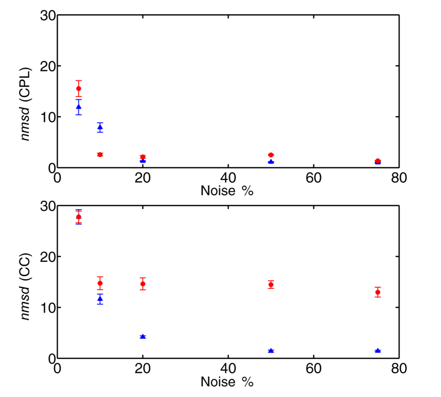
Figure 6: Variation of $nmsd$ (see text) for both CPL and CC with $\%$ of noise added to Lorenz data. Solid triangles are for white noise and solid circles are for additive red noise.

From the figure it becomes clear that the CC of the RN is not much affected by red noise contamination as the $nmsd(CC)$ remains high even with high percentage of red noise. In other words, in terms of CC, it is difficult to distinguish between a low dimensional chaotic attractor and red noise by our scheme. This implies that for RN analysis of data and surrogates where red noise is expected, such as astrophysical light curves, CC is not a good discriminating measure. On the other hand, CPL seems to be sensitive to both white and colored noise contamination and can be used as an effective discriminating statistic between data and surrogates. Hence, in the analysis of the black hole light curves below, we use only CPL as the discriminating measure. We now fix a lower limit for the value of $nmsd$ for rejecting the null hypothesis based on our results.

From Fig. 6, we find that as the noise level reaches $20\%$, the $nmsd(CPL)$ for both white and colored noise becomes very small ($<2.0$). Hence we fix a conservative limit of $10\%$ for noise level above which detection of nontrivial structures in the data is considered to be difficult. The average value of $nmsd$ corresponding to this noise level, namely $5.0$, is fixed as the threshold for rejecting the null hypothesis. It could be a point of argument whether one can fix a common threshold for nmsd applicable to all the different types of systems. This is because, sensitivity of noise can be system-specific and a good threshold $nmsd$ for one may not be so for another. Though this is true in principle, we find that the proposed threshold works in practice for a variety of systems.

In the case of synthetic time series, such as the one from the Lorenz attractor considered above, the number of variables involved and hence the embedding dimension $M$ are known a priori. However, this information is absent in the case of observational data. Just like other measures, such as $D_{2}$ and $K_{2}$, the network measures are also likely to be inaccurate if the applied embedding dimension is less than the actual dimension of the system. Two methods are commonly used to select the proper embedding dimension $M$. The more popular method is the one based on false nearest neighbor [37]. Here one looks at the changes in the nearest neighbors to a reference point as the dimension increases from $M\rightarrow M+1$. When the attractor is unfolded completely, change in nearest neighbors $\rightarrow 0$. The second method is to check for a saturated value of $D_{2}$ and then take the next higher integer value as $M$. But both these methods become difficult if the data is short and noisy. Here we show that in such situation, a network based measure can be used to find an appropriate value of $M$.

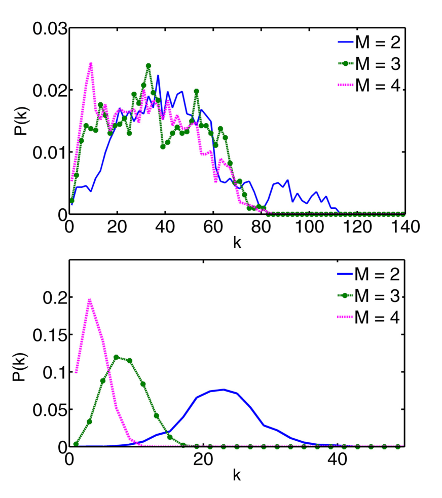
Figure 7: (Top) Degree distribution of the RN constructed from the Lorenz attractor time series with $M=2$ (solid line), $M=3$ (solid circles connected by dashed line) and $M=4$ (dotted line). (Bottom) The same for a white noise time series.

As shown by us recently [20], the degree distribution can give information regarding the number of variables required to characterize the underlying attractor. We find that for RN from chaotic time series and even colored noise, the degree distribution shows approximate convergence beyond the actual dimension of the system, a behavior identical to that of $D_{2}$. The reason is that the attractor gets confined to a sub space of the total phase space and does not change for further increase in $M$. However, for data dominated by white noise, the degree distribution keeps on shifting without showing convergence. This result is explicitly shown in Fig. 7 taking time series from the Lorenz attractor (upper panel) and white noise (lower panel) and computing the degree distribution for various $M$ values. It is also known [35] that the variation of the degree distribution with $M$ for white noise is similar to that of the surrogate data.

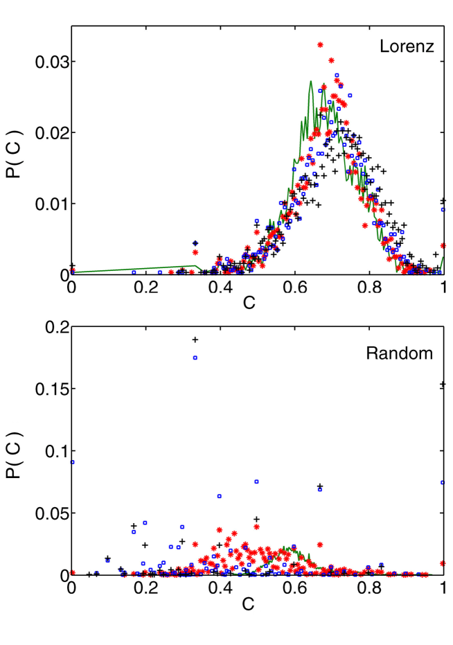
Figure 8: Probability distribution of the local clustering coefficient $P(C)$ for RNs from the Lorenz attractor time series (top panel) and pure white noise (bottom panel). In both cases, the results are shown for $M=2$ (green solid line), $M=3$ (red star points), $M=4$ (blue open squares) and $M=5$ (black crosses). While the distributions show approximate convergence for $M\geq 3$ in the top panel, the points are scattered for all $M$ values in the bottom panel.

However, the above observations regarding convergence are subjective since the distributions for two $M$ values can never coincide exactly. Hence it is desirable to have an objective measure to quantify the convergence of two distributions. Such a measure has been defined in the literature in terms of the Kullback - Leibler (K-L) divergence [38, 39]. This measure was originally introduced in probability theory to compare and quantify the difference between two probability distributions $P$ and $Q$. Specifically, the K-L divergence from $Q$ to $P$, denoted by $D_{KL}(P|Q)$, is a measure of the amount of information lost when $Q$ is used to approximate $P$. For discrete probability distributions, the K-L divergence from $Q$ to $P$ is defined as [40]:

$$D_{KL}(P|Q)=\sum_{i}P(i)\log{{P(i)}\over{Q(i)}}$$ (6)

For a continuous distribution, the summation is replaced by integration.

Though this is a useful measure, we cannot apply it directly in the case of degree distribution since the range of $k$ values is generally different for two degree distributions. To overcome this difficulty, we consider the probability distribution of the local clustering coefficient $P(C)$ over the entire RN. We find that, like the degree distribution, $P(C)$ also reflects the intrinsic nature of the time series and more importantly, it is ideal to apply the K-L measure. To get the probability $P(C)$, we compute how many nodes in the RN have a given value of $C$ and normalise this with respect to the total number of nodes in the network. The advantage here is that $C$ always varies in the unit interval and hence the comparison between two distributions is straightforward.

We first check this measure for RNs from a standard chaotic time series and white noise. For this, we construct the RN for $M$ values from $2$ to $6$. We do not consider $M>6$ since the number of nodes in the network is only $\sim 3000$. In Fig. 8, we show the $P(C)$ variation for the RNs from standard Lorenz attractor time series (upper panel) and random time series (lower panel) for $M$ values from $2$ to $5$. The difference between the upper and lower panels is obvious. For the Lorenz system, the distributions have a structure and show convergence for $M>2$ whereas, the same for a random series is scattered throughout the unit interval without showing any convergence. We have also checked this for other types of noise. For red noise, the distribution is found to converge beyond $M=3$, while for $1/f$ noise, the distribution behaves almost identical to that of white noise with no convergence in $M$. We now compute the K-L measure by comparing two distributions at a time for consecutive $M$ values using the equation:

$$D_{KL}(P_{M}|P_{M+1})=|\mu_{M}-\mu_{M+1}|+\sum_{C}P_{M}(C)\log{{P_{M}(C)}\over{P_{M+1}(C)}}$$ (7)

where $\mu_{M}$ is the average value of $C$ for dimension $M$ and $\mu_{M+1}$ is that for dimension $(M+1)$. These values are added to capture the difference due to the displacement of one profile from the other. The calculation is repeated by taking the distributions for two successive $M$ values at a time changing $M$ from 2 to 6. The values obtained are shown in Table 1. If the values show convergence above a particular $M$ value, it is taken as the required embedding dimension. For example, the values clearly show convergence for the Lorenz attractor beyond $M=2|M=3$ while they keep on fluctuating for random time series. Thus, for the Lorenz attractor and red noise, $M=3$ can be chosen as the required minimum embedding dimension from the table while no such dimension can be chosen for the white noise. This measure also provides the minimum $M$ value that should be used for computing the network measures from the RNs from real data whose dimension is unknown. We make use of this measure combined with the results obtained from RN analysis given above to distinguish between white noise and colored noise contamination in a time series.

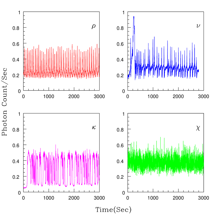
Figure 9: Representative light curves from four spectroscopic classes of the black hole system GRS1915+105. The signal amplitudes of all the light curves have been rescaled into the unit interval. Note that the signal from $\chi$ state is much weaker compared to others.

Table 1: Variation of the K-L measure obtained by comparing the probability distributions of local CC of the RNs for successive embedding dimensions for time series from Lorenz attractor, white noise and the light curves from all GRS states. The last column indicates the embedding dimension at which the measure saturates in each case. “NS” indicates no saturation.

System	$D_{KL}(P_{2}|P_{3})$	$D_{KL}(P_{3}|P_{4})$	$D_{KL}(P_{4}|P_{5})$	$D_{KL}(P_{5}|P_{6})$	$M$
Lorenz	0.1962	0.1143	0.1109	0.1004	3
White Noise	0.5498	1.6329	0.8358	1.162	NS
Red Noise	0.238	0.109	0.107	0.116	3
$\rho$	0.2115	0.1566	0.0897	0.0834	4
$\nu$	0.4687	0.1684	0.1177	0.1154	4
$\beta$	0.8207	0.1445	0.1497	0.1330	3
$\theta$	0.4182	0.1303	0.1255	0.1271	3
$\alpha$	0.6375	0.1511	0.1108	0.1144	4
$\kappa$	1.154	0.1918	0.1321	0.1287	4
$\lambda$	0.3163	0.1368	0.1306	0.1427	3
$\mu$	0.3853	0.2030	0.1223	0.1154	4
$\gamma$	1.584	1.002	0.5362	0.8904	NS
$\delta$	1.254	0.426	0.714	0.148	NS
$\phi$	2.026	0.936	0.418	0.219	NS
$\chi$	2.036	0.875	1.269	0.137	NS

4 Analysis of black hole data

In this section, we apply the network measures to analyse the X - ray light curves from the black hole binary GRS1915+105 to check how effective the network measures are in finding deterministic nonlinearity in real world data. The light curves from the black hole system have been classified into $12$ spectroscopic classes, labeled by $12$ different symbols ($\alpha$, $\beta$, $\rho$, $\nu$, $\theta$, $\kappa$, $\lambda$, $\mu$, $\delta$, $\phi$, $\gamma$ and $\chi$), by Belloni et al. [21] based on Rossi X-Ray Timing Explorer (RXTE) observation. The light curve for a given Observation ID can be obtained from the standard products [41], which provide a $0.125$ second time resolution summed over all energy channels. It is better to have continuous data without gaps though RN analysis can be done on data involving gaps which is technically more challenging. For each class, we have extracted a few continuous segments for the analysis. The light curves in all cases have been generated after rebinning to a time resolution of 1 second (to minimise noise), resulting in continuous data of length in the range $3000$ to $3500$. More details regarding the data are given elsewhere [42]. For each class, $6$ different light curves ($6$ observation IDs) were generated for the analysis.

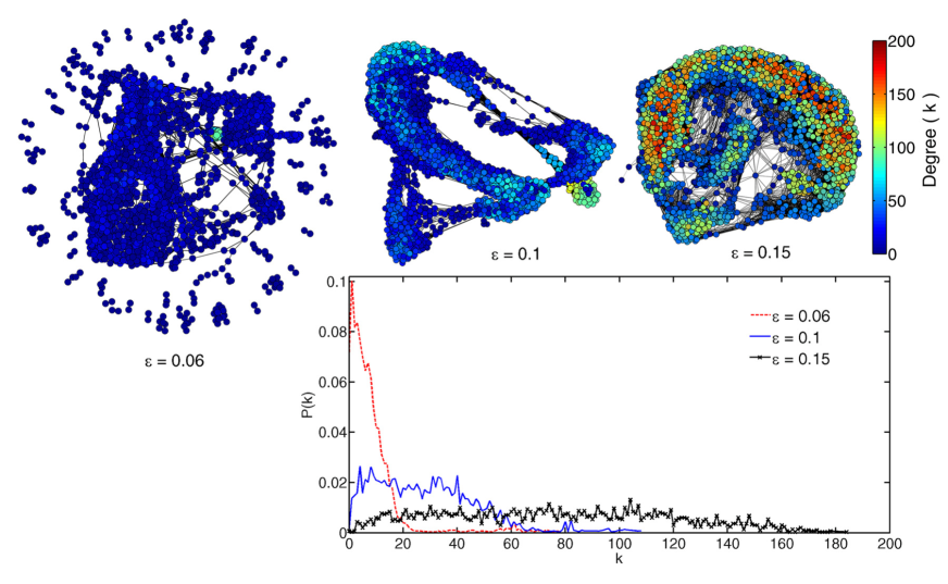
Figure 10: RNs constructed from the light curve of $\nu$ state taking $M=3$ and using three different values (as indicated) of $\epsilon$ shown in the upper panel. The degree distributions for the three networks are shown in the bottom panel. The networks and the distributions justify the selection of $\epsilon=0.1$ as the threshold for $M=3$.

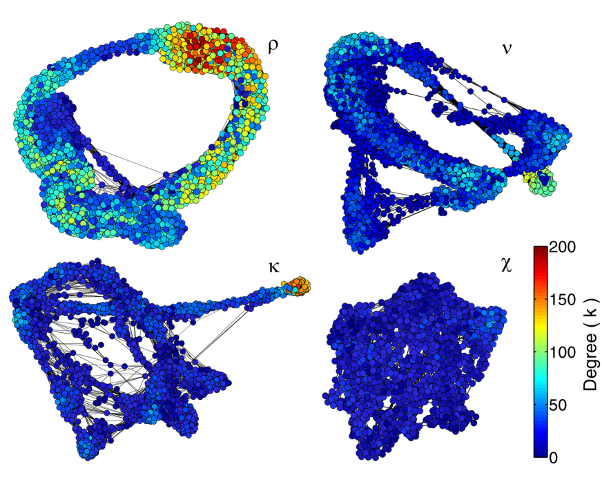
Figure 11: RNs constructed from the four light curves shown in Fig. 9 with $M=4$ and $\epsilon=0.14$. The color of a node is based on its degree as indicated in the figure.

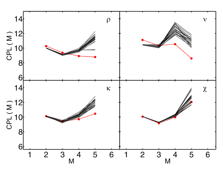
Figure 12: Results of surrogate analysis of the four representative light curves from the black hole system with CPL as the discriminating statistic. Apart from the $\chi$ state, the other states show deviations from stochastic behavior and the null hypothesis can be rejected for them.

Representative light curves from $4$ different classes are shown in Fig. 9. The black hole system appears to flip from one class to another randomly in time and it is obvious that the light curves from each class are different even visually. The complete light curves have been presented in [22], where all the light curves have been analyzed using $D_{2}$ and $K_{2}$ and classified based on a dynamical perspective and the nature of the noise content. This classification is mostly confirmed by a recurrence plot analysis [43] and very recently by a machine learning software analysis [44], where the authors developed a set of automated schemes based on supervised machine learning tools to efficiently classify the entire data set in terms of chaotic and stochastic processes. Here we check whether the analysis based on network measures can provide more accurate information on the temporal behavior of these light curves.

Before constructing the RN from the light curves we show that our approach for the threshold selection can be applied for the real world data as well. In Fig. 10 (top panel), we show the RNs constructed from a representative light curve ($\nu$) for $M=3$ with 3 values of $\epsilon$, namely, $0.06$, $0.10$ and $0.15$. In the bottom panel, the degree distributions of these RNs are also given. It is clear that $0.1$ can be taken as a reasonable choice of recurrence threshold. Thus the scheme works well for the real data as well.

The RNs constructed from the $4$ light curves shown in Fig. 9 are given in Fig. 11. All the networks appear different from each other and the network for the $\chi$ state is similar to that from a white noise. We perform the RN analysis on light curves and their surrogates from all the $12$ classes taking $6$ different light curves for each class with the CPL as the quantifying measure. Results for the above $4$ states are shown in Fig. 12. As expected, the $\chi$ state behaves identical to the white noise while the other three show deviations from purely stochastic behavior. When the average value of $nmsd$ for each class is compared with the threshold value for rejecting the null hypothesis as given above, we find that the null hypothesis can be rejected in all but $4$ states, namely, $\delta$, $\phi$, $\gamma$ and $\chi$, with the average $nmsd>5.0$ in all the other states. Note that in Fig. 12, the surrogates clearly deviate from data for $M\geq 4$ except for the $\chi$ state which is compatible with noise. We have found that the data and the surrogates deviate beyond a certain $M$ value for all the $8$ states for which the null hypothesis can be rejected.

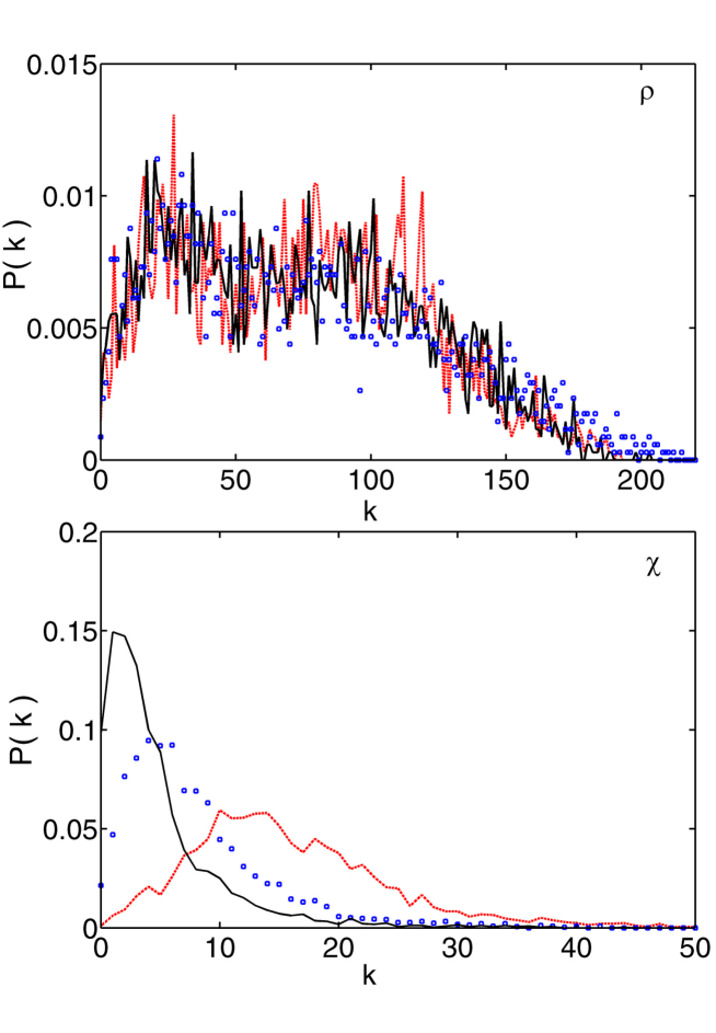
Figure 13: Degree distribution of the RNs constructed from two representative GRS light curves with $M=3$ (red dotted line), $M=4$ (blue open circles) and $M=5$ (black solid line). Note that the three degree distributions converge approximately for the $\rho$ state while they keep on shifting towards the left as $M$ increases for the $\chi$ state, which is the typical behavior of white noise.

We now compute the degree distribution of the RNs from all the light curves and find that except for the four states found to be compatible with noise in the RN analysis, all the other states show approximate convergence of the degree distribution with $M$. More importantly, the value of $M$ beyond which the convergence occurs is consistent with the $M$ value at which the data and the surrogates start deviating. The degree distributions for $2$ representative classes are shown in Fig. 13. In three states out of $8$, the convergence occurs at $M=3$ and in the remaining five, at $M=4$. To get a convergence measure with $M$, we now compute the probability distribution $P(C)$ for all the states changing $M$ from $2$ to $6$. The distributions for two GRS states are shown in Fig. 14 and the K-L measures computed from the distributions as above, are shown in Table 1 for the complete range of $M$ values for all the $12$ states. The K-L measure does not show convergence with $M$ for the $4$ states for which the null hypothesis is rejected, indicating high dimensionality. The remaining $8$ states show convergence either at $M=3$ or $M=4$, as indicated in the last column of the table.

Finally, we compute the global clustering coefficient CC for the RN using Eq. (2) for all the $12$ states taking $M=4$ and present a combined CPL-CC plot. This is shown in Fig. 15. To get a comparison with a genuine chaotic system and noise, we add the values for the RN from the Lorenz attractor, white noise and red noise. Note that the positions of the $4$ states for which the null hypothesis cannot be rejected are very close to white noise while of the remaining $8$ states, $7$ are clustered equally away from white and colored noise. Interestingly, one state $\alpha$, appears isolated with the CPL value very low compared to all other states.

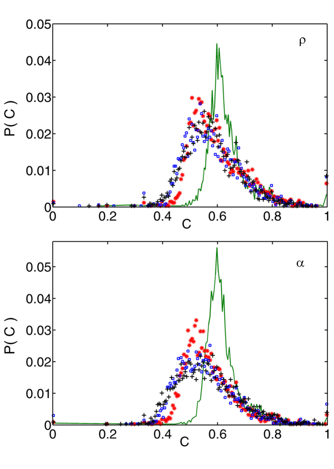
Figure 14: Probability distributions of the local clustering coefficient $C$ for RNs constructed from the light curves of two GRS states for $M=2$ (green solid line), $M=3$ (red star points), $M=4$ (blue open squares) and $M=5$ (black crosses). In both cases, the distributions tend to converge for $M\geq 4$, indicating the dimensionality of both systems as $4$.

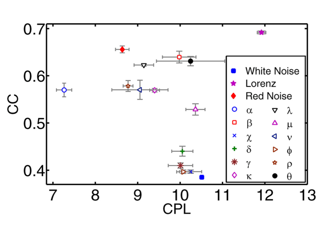
Figure 15: Combined CPL-CC plot for all the GRS light curves along with the values for the Lorenz attractor, white noise and red noise for comparison. The error bar for the GRS states represents the variation on the value over the 6 light curves while that for synthetic data is the variation for 10 different simulations.

Combining the results from surrogate analysis, the K-L convergence measure and CPL-CC plot, we can arrive at the following conclusions:

a) The four states $\delta$, $\phi$, $\gamma$ and $\chi$ are consistent with a linear-stochastic process and null hypothesis cannot be rejected for them. They show properties very similar to white noise or $1/f$ noise (which we are unable to distinguish here). Hence we consider these $4$ states to be dominated by either white noise or $1/f$ noise.

b) The remaining eight states appear to deviate from stochastic behavior with the underlying system having a finite dimensionality $M$ and are probably contaminated by some form of colored noise.

Note that by null hypothesis, we are able to reject a specific type of stochastic process, but it does not enable us to accept any other alternative. In our computations, we have used only one specific type of colored noise for detailed analysis, namely, the red noise. There are other candidates in the category of colored noise and also other different possible stochastic processes that have not been tested. Hence it is difficult to derive any further conclusions other than those given above from our numerical results on the nature of the light curves. However, by closely analyzing the values of $nmsd$ of the states for which the null hypothesis is rejected, we try to get some further information regarding the nature of their temporal behavior.

We find that the $nmsd(CPL)$ of the $8$ states for which linear stochastic behavior can be rejected fall into two different ranges. For five states $(\theta,\alpha,\beta,\lambda,\mu)$, we find the value of $nmsd$ in the range $5<nmsd<8$ and for the other three states $(\rho,\nu,\kappa)$, the values are $>9$. Since moderate contamination of colored noise tends to keep $nmsd$ high and also tends to keep $M$ value saturated, we conjecture that the former $5$ states are colored noise dominated. The latter three states can be considered to be potential candidates to search for deterministic nonlinearity. Note that the results from the present analysis are mostly in agreement with the previous analysis using $D_{2}$ and $K_{2}$ [22] where also the null hypothesis has been rejected in the same $8$ states. However, the colored noise contamination has become more evident in a couple of more states in the present analysis.

5 Discussion and conclusion

The main objectives of the entire analysis undertaken here have been threefold:

i) To test the efficiency of RN measures as discriminating statistic for hypothesis testing using surrogate data

ii) To check whether these measures are effective if the data involves both white noise and colored noise which are very common in real world systems

iii) To illustrate the possibility of a network based approach to find the dimensionality of the underlying system if the time series deviates from a purely stochastic process.

We explored three particular network measures CPL, CC and the distribution of $C$ in this analysis, with the first two used as discriminating measures. We applied a specific hypothesis that the data are derived from a linear stochastic process and then attempted to reject it using IAAFT surrogates. The time series from the standard Lorenz attractor added with different amounts of white noise, $1/f$ noise and red noise have been used to test the results of the analysis. We then found that CC is not a good discriminating measure if the data involves colored noise whereas CPL is effective in the presence of both white and colored noise. Hence we used only CPL as discriminating measure in the subsequent analysis of real data, the light curves from $12$ spectroscopic classes of the black hole system GRS 1915+105.

The real advantage of using network measures is that they can be accurately computed from a lower number of nodes in the network, compared to the number of data points required for computing $D_{2}$ and $K_{2}$. One novel aspect of the present analysis is the result that the network approach can be combined with a new measure derived from the probability distribution of the clustering coefficient to get information regarding the dimension of the underlying system in the time series. Using this measure we are able to identify the dimension of the light curves from all the temporal states for which the null hypothesis can be rejected. Thus we find that a network approach with CPL as discriminating measure and the convergence measure based on $P(C)$ is better suited to study the temporal properties of time series from the real world.

Though our main motivation in the present analysis was to study application of network measures as tools to analyze real data, we think it is appropriate to mention what new information we have gained regarding the nature of light curves with this analysis. The present study mostly supports the previous one with null hypothesis rejected for the same states. One additional information of the present approach is the possibility of deriving the dimension also from a time series with a limited number of data points and a better information regarding colored noise contamination in various states. The astrophysical reason of why very few black hole systems show different spectroscopic classes (with qualitatively different temporal behavior) and random flippings between these classes, is still an open question and an active field of research. The result that a few states may be deterministic and nonlinear does not in any way imply that there is evidence for chaos in the system. It only implies that the accretion process responsible for the generation of the light curves in these states may have some underlying dynamics which can somehow be represented by a system of coupled nonlinear differential equations. Chaos, of course, is a more exciting prospect, but warrants more specific criteria on the part of the system apart from nonlinearity. We are of the opinion that detecting chaos from limited real world data immersed in noise using any of the time series methods is extremely difficult (if at all possible). In the present context, it requires the development of, at least, a truncated model of the accretion process in which critical changes in one or two control parameters can bring about qualitative changes in the nature of the light curves. This is, by far, a very challenging task.

Acknowledgements

We thank one of the anonymous referees for a thorough review of the manuscript and suggesting many changes to improve the presentation. RJ and KPH acknowledge the financial support from Science and Engineering Research Board (SERB), Govt. of India in the form of a Research Project No SR/S2/HEP-27/2012. KPH acknowledges the computing facilities in IUCAA, Pune.

For graphical representation of networks, we use the GEPHI software:
(https://gephi.org/).

References

- [1] H. Kantz and T. Schreiber, Nonlinear Time Series Analysis, (Cambridge University Press, Cambridge, 2004)
- [2] J. C. Sprott, Chaos and Time Series Analysis, (Oxford University Press, Oxford, 2003)
- [3] T. Schreiber and A. Schmitz, Discriminating power of measures for nonlinearity in a time series, Phys. Rev. E 55, 5443(1997)
- [4] J. Theiler, S. Eubank, A. Longtin, B. Galdrikian and J. Farmer, Testing for nonlinearity in time series: The method of surrogate data, Physica D 58, 77–94(1992)
- [5] J. F. Donges, R. V. Donner and J. Kurths, Testing time series irreversibility using complex network methods, Europhys. Lett. 102, 10004(2013)
- [6] L. Lacasa, A. Nunez, E. Roldan, J. M. R. Porrondo and B. Luque, Time series irreversibility: a visibility graph approch, Eur. Phys. J. B 85, 217(2012)
- [7] D. Kugiumtzis, Test your surrogate data before you test for nonlinearity, Phys. Rev. E 60, 2808(1999)
- [8] T. Schreiber and A. Schmitz, Improved surrogate data for nonlinearity tests, Phys. Rev. Lett. 77, 635(1996)
- [9] T. Schreiber and A. Schmitz, Surrogate time series, Physica D 142, 346(2000)
- [10] T. Nakamura, M. Small and Y. Hirata, Testing for nonlinearity in irregular fluctuations with long-term trends, Phys. Rev. E 74, 026205(2006)
- [11] J. H. Lucio, R. Valdes and L. R. Rodriguez, Improvements to surrogate data methods for nonstationary time series, Phys. Rev. E 85, 056202(2012)
- [12] T. Nakamura and M. Small, Small-shuffle surrogate data: Testing for dynamics in fluctuating data with trends, Phys. Rev. E 72, 056216(2005)
- [13] X. Luo, T. Nakamura and M. Small, Surrogate test to distinguish between pseudo periodic time series data, Phys. Rev. E 71, 026230(2005)
- [14] M. Thiel, M. C. Romano, J. Kurths, M. Rolfs and R. Kliegl, Generating surrogates from recurrences, Phil. Trans. Royal Soc. A 366, 545(2008)
- [15] R. Hegger, H. Kantz and T. Schreiber, Practical implementation of nonlinear time series methods: The TISEAN package, CHAOS 9, 413(1999)
- [16] J. C. Sprott and G. Rowlands, Improved correlation dimension calculation, Int. J. Bif. Chaos 11, 1865(2001)
- [17] P. Grassberger and I. Procaccia, Measuring the strangeness of strange attractors, Physica D 9, 189-208(1983)
- [18] N. P. Subramaniyam and J. Hyttinen, Characterization of dynamical systems under noise using recurrence networks: Application to simulated and EEG data, Phys. Lett. A 378, 3464–74(2014)
- [19] N. P. Subramaniyam and J. Hyttinen, Dynamics of intra cranial EEG recordings from epilepsy patients using univariate and bivariate recurrence networks, Phys. Rev. E 91, 022927(2015)
- [20] Rinku Jacob, K. P. Harikrishnan, R. Misra and G. Ambika, Characterization of chaotic attractors under noise: A recurrence network perspective, Comm. Nonlinear Sci. and Num. Simul. 41, 32-47(2016)
- [21] T. Belloni, M. Klein-Wolt, M. Mendez, M. van der Klis and J. van Paradjis, A model-independent analysis of the variability of GRS 1915+105, Astronomy and Astrophys. 355, 271–290(2000)
- [22] K. P. Harikrishnan, R. Misra and G. Ambika, Nonlinear time series analysis of the light curves from the black hole system GRS 1915+105, Research in Astr. and Astrophys. 11, 71–90(2011)
- [23] J. F. Donges, J. Heitzig, R. V. Donner and J. Kurths, Analytical framework for recurrence network analysis of time series, Phys. Rev. E 85, 046105(2012)
- [24] J. P. Eckmann, S. O. Kamphorst and D. Ruelle, Recurrence plot of dynamical systems, Europhys Letters 5, 973-977(1987)
- [25] N. Marwan, J. F. Donges, Y. Zou, R. V. Donner and J. Kurths, Complex network approach for recurrence analysis of time series, Phys. Lett. A 373, 4246-4254(2009)
- [26] J. P. Zbilut and C. L. Webber Jr., Embeddings and delays as derived from quantification of recurrence plots, Phys. Lett. A 171, 199–203(1992)
- [27] S. H. Strogatz, Exploring complex networks, Nature 410, 268–76(2001)
- [28] M. E. J. Newman, The structure and function of complex networks, SIAM Rev. 45, 167–256(2003)
- [29] R. V. Donner, Y. Zou, J. F. Donges, N. Marwan and J. Kurths, Recurrence networks: A novel paradigm for nonlinear time series analysis, New J. Phys. 12, 033025(2010)
- [30] J. Zhang and M. Small, Complex networks from pseudoperiodic time series: topology versus dynamics, Phys. Rev. Lett. 96, 238701(2006)
- [31] X. Xu, J. Zhang and M. Small, Super family phenomena and motifs of networks induced from time series, Proc. Natl. Acad. Sci. USA 105, 19601-5(2008)
- [32] R. V. Donner, M. Small, J. F. Donges, N. Marwan, Y. Zou, R. Xiang and J. Kurths, Recurrence based time series analysis by means of complex network methods, Int. J. Bif. Chaos 21, 1019-46(2011)
- [33] K. P. Harikrishnan, R. Misra, G. Ambika and A. K. Kembhavi, A non-subjective approach to the GP algorithm for analysing noisy time series, Physica D 215, 137-145(2006)
- [34] R. V. Donner, J. Heitzig, J. F. Donges, Y. Zou, N. Marwan and J. Kurths, The geometry of chaotic dynamics-A complex network perspective, European Phys. J. B 84, 653-672(2011)
- [35] Rinku Jacob, K. P. Harikrishnan, R. Misra and G. Ambika, Uniform framework for the recurrence-network analysis of chaotic time series, Phys. Rev. E 93, 012202(2016)
- [36] M. E. J. Newman, Networks: An introduction, (Oxford University Press, Oxford, 2010)
- [37] M. B. Kennel, R. Brown and H. D. I. Aberbanel, Determining minimum embedding dimension using a geometrical construction, Phys. Rev. E 45, 3403(1992)
- [38] S. Kullback and R. A.Leibler, On information and sufficiency, Ann. Math. Stat. 22, 79-86(1951)
- [39] S. Kullback, Information Theory and Statistics, (John Wiley, NewYork, 1959)
- [40] D. J. C. Mackay, Information Theory, Inference and Learning Algorithms, (Cambridge Univ. Press, Cambridge, 2003)
- [41] The light curves can be derived from: http://heasarc.gsfc.nasa.gov/docs/xte/recipes/stdprod-guide.html
- [42] R. Misra, K. P. Harikrishnan, B. Mukhopadhyay, G. Ambika and A. K. Kembhavi, Chaotic behavior of the black hole system GRS1915+105, Astrophys. J. 609, 313(2004)
- [43] P. Sukova, M. Grzedzielski and A. Janiuk, Chaotic and stochastic processes in the accretion flows of the black hole X-ray binaries revealed by recurrence analysis, Astron. and Astrophys. 586, A143(2016)
- [44] D. Huppenkothen, L. M. Heil, D. W. Hogg and A. Mueller, Using machine learning to explore the long-term evolution of GRS 1915+105, Mon. Not. Roy. Astr. Soc. 466(2), 2364(2017)