Faster Betweenness Centrality Updates in Evolving Networks

Abstract.

Finding central nodes is a fundamental problem in network analysis. Betweenness centrality is a well-known measure which quantifies the importance of a node based on the fraction of shortest paths going though it. Due to the dynamic nature of many today’s networks, algorithms that quickly update centrality scores have become a necessity. For betweenness, several dynamic algorithms have been proposed over the years, targeting different update types (incremental- and decremental-only, fully-dynamic). In this paper we introduce a new dynamic algorithm for updating betweenness centrality after an edge insertion or an edge weight decrease. Our method is a combination of two independent contributions: a faster algorithm for updating pairwise distances as well as number of shortest paths, and a faster algorithm for updating dependencies. Whereas the worst-case running time of our algorithm is the same as recomputation, our techniques considerably reduce the number of operations performed by existing dynamic betweenness algorithms. Our experimental evaluation on a variety of real-world networks reveals that our approach is significantly faster than the current state-of-the-art dynamic algorithms, approximately by one order of magnitude on average.

1. Introduction

Over the last years, increasing attention has been devoted to the analysis of complex networks. A common sub-problem for many graph based applications is to identify the most central nodes in a network. Examples include facility location [13], marketing strategies [12] and identification of key infrastructure nodes as well as disease propagation control and crime prevention [1]. As the meaning of “central” heavily depends on the context, various centrality measures have been proposed (see [4] for an overview). Betweenness centrality is a well-known measure which ranks nodes according to their participation in the shortest paths of the network. Formally, the betweenness of a node $v$ is defined as $c_{B}(v)=\sum_{s\neq v\neq t}\frac{\sigma_{st}(v)}{\sigma_{st}}$, where $\sigma_{st}$ is the number of shortest paths between two nodes $s$ and $t$ and $\sigma_{st}(v)$ is the number of these paths that go through node $v$. The fastest algorithm for computing betweenness centrality is due to Brandes [6], which we refer to as BA, from Brandes’s algorithm. This algorithm is composed of two parts: an augmented APSP (all-pairs shortest paths) step, where pairwise distances and shortest paths are computed, and a dependency accumulation step, where the actual betweenness scores are computed. The augmented APSP is computed by running a SSSP (single-source shortest paths) computation from each node $s$ and the dependency accumulation is performed by traversing only once the edges that lie in shortest paths between $s$ and the other nodes. Therefore, BA requires $\Theta(|V||E|)$ time on unweighted and $\Theta(|V||E|+|V|^{2}\log|V|)$ time on weighted graphs (i.e. the time of running $n$ SSSPs).

Networks such as the Web graph and social networks continuously undergo changes. Since an update in the graph might affect only a small fraction of nodes, recomputing betweenness with BA after each update would be very inefficient. For this reason, several dynamic algorithms have been proposed over the last years [9, 14, 11]. As BA, these approaches usually solve two sub-tasks: the update of the augmented APSP data structures and the update of the betweenness scores. Although none of these algorithms is in general asymptotically faster than recomputation with BA, good speedups over BA have been reported for some of them, in particular for [11] and [14]. Nonetheless, an exhaustive comparison of these methods is missing in the literature.

In our paper, we only consider incremental updates, i.e. edge insertions or edge weight decreases (node insertions can be handled treating the new node as an isolated node and adding its neighboring edges one by one). Although it might seem reductive to only consider these kinds of updates, it is important to note that several real-world dynamic networks evolve only this way and do not shrink. For example, in a co-authorship network, a new author (node) or a new edge (coauthored publication) might be added to the network, but existing nodes or edges will not disappear. Another possible application is the centrality maximization problem, which consists in finding a set of edges that, if added to the graph, would maximize the centrality of a certain node. The problem can be approximated with a heuristic [7], which requires to add several edges to the graph and to recompute distances after each edge insertion.

Our contribution

We present a new algorithm for updating betweenness centrality after an edge insertion or an edge weight decrease. Our method is a combination of two contributions: a new dynamic algorithm for the augmented APSP, and a new approach for updating the betweenness scores. Based on properties of the newly-created shortest paths, our dynamic APSP algorithm efficiently identifies the node pairs affected by the edge update (i.e. those for which the distance and/or number of shortest paths change as a consequence of the update). The betweenness update method works by accumulating values in a fashion similar to that of BA. However, differently from BA, our method only processes nodes that lie in shortest paths between affected pairs.

We compare our new approach with two of the dynamic algorithms for which the best speedups over recomputation have been reported in the literature, i.e. KWCC [11] and KDB [14]. Compared to them, our algorithm for the augmented APSP update is asymptotically faster on dense graphs: $O(|V|^{2})$ in the worst case versus $O(|V||E|)$. This is due to the fact that we iterate over the edges between affected nodes only once, whereas KDB and KWCC do it several times. Moreover, our dependency update works also for weighted graphs (whereas KDB does not) and it is asymptotically faster than the dependency update of KWCC for sparse graphs ($O(|V||E|+|V|\log|V|)$ in the worst case versus $O(|V|^{3})$).

Our experimental evaluation on a variety of real-world networks reveals that our approach is significantly faster than both KDB and KWCC, on average by a factor 14.7 and 7.4, respectively.

2. Preliminaries

2.1. Notation

Let $G=(V,E,\omega)$ be a graph with node set $V=V(G)$, edge set $E=E(G)$ and edge weights $\omega:E\rightarrow\mathbb{R}_{>0}$. In the following we will use $n:=|V|$ to denote the number of nodes and $m:=|E|$ for the number of edges. Let $d(s,t)$ be the shortest-path distance between any two nodes $s,t\in V$. On a shortest path from $s$ to $t$ in $G$, we say $w$ is a predecessor of $t$, or $t$ is a successor of $w$, if $(w,t)\in E$ and $d(s,w)+\omega(w,t)=d(s,t)$. We denote the set of predecessors of $t$ as $P_{s}(t)$. For a given source node $s\in V$, we call the graph composed of the nodes reachable from $s$ and the edges that lie in at least one shortest path from $s$ to any other node the SSSP DAG of $s$. We use $\sigma_{st}$ to denote the number of shortest paths between $s$ and $t$ and we use $\sigma_{st}(v)$ for the number of shortest paths between $s$ and $t$ that go through $v$. Then, the betweenness centrality $c_{B}(v)$ of a node $v$ is defined as: $c_{B}(v)=\sum_{s\neq v\neq t}\frac{\sigma_{st}(v)}{\sigma_{st}}$.

Our goal is to keep track of the betweenness scores of all nodes after an update $(u,v,\omega^{\prime}(u,v))$ in the graph, which could either be an edge insertion or an edge weight decrease. We use $G^{\prime}=(V,E^{\prime},\omega^{\prime})$ to denote the new graph after the edge update and $d^{\prime}$, $\sigma^{\prime}$ and $P^{\prime}$ to denote the new distances, numbers of shortest paths and sets of predecessors, respectively. Also, we define the set of affected sources $S(t)$ of a node $t\in V$ as $\{s\in V:d(s,t)>d^{\prime}(s,t)\vee\sigma_{st}\neq\sigma^{\prime}_{st}\}$. Analogously, we define the set of affected targets of $s\in V$ as $T(s):=\{t\in V:d(s,t)>d^{\prime}(s,t)\vee\sigma_{st}\neq\sigma^{\prime}_{st}\}$. In the following we will assume $G$ to be directed. However, the algorithms can be easily extended to undirected graphs.

2.2. Related Work

The basic idea of dynamic betweenness algorithms is to keep track of the old betweenness scores (and additional data structures) and efficiently update the information after some modification in the graph. Based on the type of updates they can handle, dynamic algorithms are classified as incremental (only edge insertions and weight decreases), decremental (only edge deletions and weight increases) or fully-dynamic (all kinds of edge updates). However, one commonality of all these approaches is that they build on the techniques used by BA [6], which we therefore describe in Section 3 in more detail.

The approach proposed by Green et al. [9] for unweighted graphs maintains all previously calculated betweenness values and additional information, such as pairwise distances, number of shortest paths and lists of predecessors of each node in the shortest paths from each source node $s\in V$. Using this information, the algorithm tries to limit the recomputation to the nodes whose betweenness has been affected by the edge insertion. Kourtellis et al. [14] modify the approach by Green et al. [9] in order to reduce the memory requirements from $O(nm)$ to $O(n^{2})$. Instead of being stored, the predecessors are recomputed every time the algorithm requires them. The authors show that not only using less memory allows them to scale to larger graphs, but their approach (which we refer to as KDB, from the authors’s initials) turns out to be also faster than the one by Green et al. [9] in practice (most likely because of the cost of maintaining the data structure of the algorithm by Green et al.).

Kas et al. [11] extend an existing algorithm for the dynamic all-pairs shortest paths (APSP) problem by Ramalingam and Reps [21] to also update betweenness scores. Differently from the previous two approaches, this algorithm can handle also weighted graphs. Although good speedups have been reported for this approach, no experimental evaluation compares its performance with that of the approaches by Green et al. [9] and Kourtellis et al. [14]. We refer to this algorithm as KWCC, from the authors’s initials.

Nasre et al. [19] compare the distances between each node pair before and after the update and then recompute the dependencies from scratch as in BA (see Section 3). Although this algorithm is faster than recomputation on some graph classes (i.e. when only edge insertions are allowed and the graph is sparse and weighted), it was shown in [3] that its practical performance is much worse than that of the algorithm proposed by Green et al. [9]. This is quite intuitive, since recomputing all dependencies requires $\Omega(n^{2})$ time independently of the number of nodes that are actually affected by the insertion.

Pontecorvi and Ramachandran [20] extend existing fully-dynamic APSP algorithms with new data structures to update all shortest paths and then recompute dependencies as in BA. To our knowledge, this algorithm has never been implemented, probably because of the quite complicated data structures it requires. Also, since it recomputes dependencies from scratch as Nasre et al. [19], we expect its practical performance to be similar.

Differently from the other algorithms, the approach by Lee et al. [16] is not based on dynamic APSP algorithms. The idea is to decompose the graph into its biconnected components and then recompute the betweenness values from scratch only for the nodes in the component affected by the update. Although this allows for a smaller memory requirement ($\Theta(m)$ versus $\Omega(n^{2})$ needed by the other approaches), the speedups on recomputation reported in [16] are significantly worse than those reported for example by Kourtellis et al. [14].

To summarize, KDB [14] and KWCC [11] are the most promising methods for a comparison with our new algorithm. For this reason, we will describe them in more detail in Section 4 and Section 5 and evaluate them in our experiments.

Since computing betweenness exactly can be too expensive for large networks, several approximation algorithms and heuristics have been introduced in the literature [5, 8, 22, 23] and, recently, also dynamic algorithms that update an approximation of betweenness centrality have been proposed [2, 3, 10, 23]. However, we will not consider them in our experimental evaluation since our focus here is on exact methods.

3. Brandes’s algorithm (BA)

Betweenness centrality can be easily computed in time $\Theta(n^{3})$ by simply applying its definition. In 2001, Brandes proposed an algorithm (BA) [6] which requires time $\Theta(nm)$ for unweighted and $\Theta(n(m+n\log n))$ for weighted graphs, i.e. the time of computing $n$ single-source shortest paths (SSSPs). The algorithm is composed of two parts: the augmented APSP computation phase based on $n$ SSSPs and the dependency accumulation phase. As dynamic algorithms based on BA build on these two steps as well, we explain them now in more detail.

Augmented APSP

In this first part, BA needs to perform an augmented APSP, meaning that instead of simply computing distances between all node pairs $(s,t)$, it also finds the number of shortest paths $\sigma_{st}$ and the set of predecessors $P_{s}(t)$. This can be done while computing an SSSP from each node $s$ (i.e. BFS for unweighted and Dijkstra for weighted graphs). When a node $w$ is extracted from the SSSP (priority) queue, BA computes $P_{s}(w)$ as $\{v:(v,w)\in E\,\wedge\,d(s,w)=d(s,v)+\omega(v,w)\}$ and $\sigma_{sw}$ as $\sum_{v\in P_{s}(w)}\sigma_{sv}$.

Dependency accumulation

Brandes defines the one-side dependency of a node $s$ on a node $v$ as $\delta_{s\bullet}(v):=\sum_{t\neq v}\sigma_{st}(v)/\sigma_{st}$. It can be proven [6] that

$$\delta_{s\bullet}(v)=\sum_{w:v\in P_{s}(w)}\frac{\sigma_{sv}}{\sigma_{sw}}(1+\delta_{s\bullet}(w)),\ \ \ \ \forall s,v\in V$$ (1)

Intuitively, the term $\delta_{s\bullet}(w)$ in Eq. (1) represents the contribution of the sub-DAG (of the SSSP DAG of $s$) rooted in $w$ to the betweenness of $v$, whereas the term $1$ is the contribution of $w$ itself. For all nodes $v$ such that $\{w:v\in P_{s}(w)\}=\emptyset$ (i.e. the nodes that have no successors), we know that $\delta_{s\bullet}(v)=0$. Starting from these nodes, we can compute $\delta_{s\bullet}(v)\ \forall v\in V$ by “walking up” the SSSP DAG rooted in $s$, using Eq. (1). Notice that it is fundamental that we process the nodes in order of decreasing distance from $s$, because to correctly compute $\delta_{s\bullet}(v)$, we need to know $\delta_{s\bullet}(w)$ for all successors of $v$. This can be done by inserting the nodes into a stack as soon as they are extracted from the SSSP (priority) queue in the first step. The betweenness of $v$ is then simply computed as $\sum_{s\neq v}\delta_{s\bullet}(v)$.

4. Dynamic augmented APSP

As mentioned in Section 3, also dynamic algorithms based on BA build on its two steps. In the following, we will see how KDB [14] and KWCC [11] update the augmented APSP data structures (i.e. distances and number of shortest paths) after an edge insertion or a weight decrease. One difference between these two approaches is that KDB does not store the predecessors explicitly, whereas KWCC does. However, since in [14] it was shown that keeping track of the predecessors only introduces overhead, we report a slightly-modified version of KWCC that recomputes them “on the fly” when needed (we will also use this version in our experiments in Section 7). We will then introduce our new approach in Section 4.3.

4.1. Algorithm by Kourtellis et al. (KDB)

Let $(u,v)$ be the new edge inserted into $G$ (we recall that KDB works only on unweighted graphs, so edge weight modifications are not supported). For each source node $s\in V$, there are three possibilities: $(i)$ $d(s,u)=d(s,v)$, $(ii)$ $|d(s,u)-d(s,v)|=1$ and $(iii)$ $|d(s,u)-d(s,v)|>1$ (in case $(ii)$ and $(iii)$, let us assume that $d(s,u)<d(s,v)$ without loss of generality). We recall that $d$ is the distance before the edge insertion.

In the first case, it is easy to see that the insertion does not affect any shortest path rooted in $s$, and therefore nothing needs to be updated for $s$.

In case $(ii)$, the distance between $s$ and the other nodes is not affected, since there already existed an alternative shortest-path from $s$ to $v$. However, the insertion creates new shortest paths from $s$ to to $v$ and consequently to all the nodes $t$ in the sub-DAG (of the SSSP DAG from $s$) rooted in $v$. To account for this, for each of these nodes $t$, we add $\sigma_{su}\cdot\sigma_{vt}$ to the old value of $\sigma_{st}$ (where $\sigma_{su}\cdot\sigma_{vt}$ is the number of new shortest paths between $s$ and $t$ going through $(u,v)$).

Finally, in case $(iii)$, a part of the sub-DAG rooted in $v$ might get closer to $s$. This case is handled with a BFS traversal rooted in $v$. In the traversal, all neighbors $y$ of nodes $x$ extracted from the BFS queue are examined and all the ones such that $d(s,y)\geq d^{\prime}(s,x)$ are also enqueued. For each traversed node $y$, the new distance $d^{\prime}(s,y)$ is computed as $\min_{z:(z,y)\in E}d^{\prime}(s,z)+1$ and the number of shortest paths $\sigma^{\prime}_{sy}$ as $\sum_{z\in P^{\prime}_{s}(y)}\sigma_{sz}$.

4.2. Algorithm by Kas et al. (KWCC)

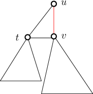
Figure 1. Insertion of $(u,v)$.

KWCC updates the augmented APSP based on a dynamic APSP algorithm by Ramalingam and Reps [21]. Instead of checking for each source $s$ whether the new edge (or the weight decrease) changes the SSSP DAG rooted in $s$, KWCC first identifies the affected sources $S=\{s:d(s,v)\geq d(s,u)+\omega^{\prime}(u,v)\}$. These are exactly the nodes for which there is some change in the SSSP DAG. The affected sources are identified by running a pruned BFS rooted in $u$ on $G$ transposed (i.e. the graph obtained by reversing the direction of edges in $G$). For each node $s$ traversed in the BFS, KWCC checks whether the neighbors of $s$ are also affected sources and, if not, it does not continue the traversal from them. Notice that even on weighted graphs, a (pruned) BFS is sufficient since we already know all distances to $v$ and we can basically sidestep the use of a priority queue.

Once all affected sources $s$ are identified, KWCC starts a pruned BFS rooted in $v$ for each of them. In the pruned BFS, only nodes $t$ such that $d(s,t)\geq d(s,u)+\omega^{\prime}(u,v)+d(v,t)$ are traversed (the affected targets of $s$). The new distance $d^{\prime}(s,t)$ is set to $d(s,u)+\omega^{\prime}(u,v)+d(v,t)$ and the new number of shortest paths $\sigma^{\prime}(s,t)$ is set to $\sum_{z\in P^{\prime}_{s}(t)}\sigma_{sz}$ as in KDB. Compared to KDB, the augmented APSP update of KWCC requires fewer operations. First, it efficiently identifies the affected sources instead of checking all nodes. Second, in case $(iii)$, KDB might traverse more nodes than KWCC. For example, assume $(u,v)$ is a new edge and the resulting SSSP DAG of $u$ is as in Figure 1. Then, KWCC will prune the BFS in $t$, since $d(u,t)<d(u,v)+d(v,t)$, skipping all the SSSP DAGs rooted in $t$. On the contrary, KDB will traverse the whole subtree rooted in $t$, although neither the distances nor the number of shortest paths from $u$ to those nodes are affected. The reason for this will be made clearer in Section 5.1.

4.3. Faster augmented APSP update

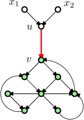
Figure 2. Affected targets (in green) and affected sources ($x_{1},x_{2},u$).

To explain our idea for improving the APSP update step, let us start with an example, shown in Figure 2. The insertion of $(u,v)$ decreases the distance from nodes $x_{1},x_{2},u$ to all the nodes shown in green. KWCC would first identify the affected sources $S=\{x_{1},x_{2},u\}$ and, for each of them, run a pruned BFS rooted in $v$. This means we are repeating almost exactly the same procedure for each of the affected sources. We clearly have to update the distances and number of shortest paths between each affected source and the affected targets (and this cannot be avoided). However, KWCC also goes through the outgoing edges of each affected target multiple times, leading to a worst-case running time of $O(mn)$. Our basic idea is to avoid this redundancy and is based on the following proposition (a similar result was proven also in [18]).

Proposition .

Let $t\in V$ and $y\in P_{v}(t)$ be given. Then, $S(t)\subseteq S(y)$.

Proof.

Let $s$ be any node in $S(t)$, i.e. either $d^{\prime}(s,t)=d(s,t)$ and $\sigma^{\prime}_{st}\neq\sigma_{st}$ (case $(i)$), or $d^{\prime}(s,t)<d(s,t)$ (case $(ii)$). We want to show that $s\in S(y)$.

Before proving this, we show that $y$ has to be in $P^{\prime}_{s}(t)$. In fact, if $s\in S(t)$, there have to be shortest paths between $s$ and $t$ going through $(u,v)$, i.e. $d^{\prime}(s,t)=d(s,u)+\omega^{\prime}(u,v)+d(v,t)$. On the other hand, we know $y\in P_{v}(t)$ and thus

$$d^{\prime}(s,t)=d(s,u)+\omega^{\prime}(u,v)+d(v,y)+\omega(y,t).$$ (2)

Now, $d(s,u)+\omega^{\prime}(u,v)+d(v,y)$ cannot be larger than $d^{\prime}(s,y)$, or this would mean that $d^{\prime}(s,t)>d^{\prime}(s,v)+\omega(y,t)$, which contradicts the triangle inequality. Also, $d(s,u)+\omega^{\prime}(u,v)+d(v,y)$ cannot be smaller than $d^{\prime}(s,y)$ by definition of distance. Thus, $d^{\prime}(s,y)=d(s,u)+\omega^{\prime}(u,v)+d(v,y)$. If we substitute this in Eq. (2), we obtain $d^{\prime}(s,t)=d^{\prime}(s,y)+\omega(y,t)$, which means $y\in P^{\prime}_{s}(t)$.

Now, let us consider case $(i)$. We have two options: either $y$ was a predecessor of $t$ from $s$ also before the edge update, i.e. $y\in P_{s}(t)$, or it was not. If it was not, it means $d(s,y)+\omega(y,t)>d(s,t)=d^{\prime}(s,t)=d^{\prime}(s,y)+\omega(y,t)$, which implies $d(s,y)>d^{\prime}(s,y)$ and thus $s\in S(y)$. If it was, we can similarly show that $d(s,y)=d^{\prime}(s,y)$. Since we have seen before that $d^{\prime}(s,y)=d(s,u)+\omega^{\prime}(u,v)+d(v,y)$, there has to be at least one new shortest path from $s$ to $y$ in $G^{\prime}$ going through $(u,v)$, which means $\sigma^{\prime}_{sy}>\sigma_{sy}$ and therefore $s\in S(y)$.

Case $(ii)$ can be easily proven by contradiction. We know $d(s,t)\leq d(s,y)+\omega(y,t)$ (by the triangle inequality) and that $\omega^{\prime}(y,t)=\omega(y,t)$. Thus, if it were true that $d(s,y)=d^{\prime}(s,y)$ then

$$d(s,t)\leq d(s,y)+\omega(y,t)=d^{\prime}(s,y)+\omega(y,t)=d^{\prime}(s,t),$$ (3)

which contradicts our hypothesis that $d^{\prime}(s,t)<d(s,t)$ (case $(ii)$). Thus, $d(s,y)\neq d^{\prime}(s,y)$. Since pairwise distances in $G^{\prime}$ can only be equal to or shorter than pairwise distances in $G$, $d(s,y)\neq d^{\prime}(s,y)$ implies $d(s,y)>d^{\prime}(s,y)$ and thus $s\in S(y)$.

∎

In particular, this implies that $S(t)\subseteq S(v)$ for each $t\in T(u)$. Consequently, it is sufficient to compute $S(v)$ and $T(u)$ once via two pruned BFSs. Our approach is described in Algorithm 1. The pruned BFS to compute $S(v)$ is performed in Line 1. Then, a pruned BFS from $v$ is executed, whereby for each $t\in T(u)$ we store one of its predecessors $p(t)$ in the BFS (Line 1).

Let $d^{\star}(s,t)$ be the length of a shortest path between $s$ and $t$ going through $(u,v)$, i.e. $d^{\star}(s,t):=d(s,u)+\omega^{\prime}(u,v)+d(v,t)$. To finally compute $S(t)$ all that is left to do is to test whether $d^{\star}(s,t)\leq d(s,t)$ for each $s\in S(p(t))$ once we remove $t$ from the queue (Lines 1 - 1). Note that this implies that $S(p(t))$ was already computed. In case $d^{\star}(s,t)<d(s,t)$, the path from $s$ to $t$ via edge $(u,v)$ is shorter than before and therefore we set $d^{\prime}(s,t)$ to $d^{\star}(s,t)$ and $\sigma^{\prime}_{st}$ to $\sigma_{su}\cdot\sigma_{vt}$, since all new shortest paths now go through $(u,v)$). Also in case of equality ($d^{\star}(s,t)=d(s,t)$), $s$ is in $S(t)$, since its number of shortest paths has changed. Consequently we set $\sigma^{\prime}_{st}$ to $\sigma_{st}+\sigma_{su}\cdot\sigma_{vt}$ (since in this case also old shortest paths are still valid). If $d^{\star}(s,t)>d(s,t)$, the edge $(u,v)$ does not lie on any shortest path from $s$ to $t$, hence $s\notin S(t)$ (and $s$ is not added to $S(t)$ in Lines 1 - 1).

Input : Graph $G=(V,E)$, edge insertion/weight decrease $(u,v,\omega^{\prime}(u,v))$, $d(s,t)$, $\sigma_{st},\ \forall(s,t)\in V^{2}$

Output : Updated $d^{\prime}(s,t)$, $\sigma^{\prime}_{st},\ \forall(s,t)\in V^{2}$

Assume : Initially $d^{\prime}(s,t)=d(s,t)$ and $\sigma^{\prime}_{st}=\sigma_{st}\ \ \forall(s,t)\in V^{2}$

1 $vis(v)\leftarrow\text{false}\ \forall v\in V$;

2 if $\omega^{\prime}(u,v)\leq d(u,v)$ then

3       $S(v)\leftarrow$ findAffectedSources($G,(u,v,\omega^{\prime}(u,v))$);

4       $d(u,v)\leftarrow\omega^{\prime}(u,v)$;

5       $Q\leftarrow\emptyset$;

6       $p(v)\leftarrow v$;

7       $Q.push(v)$;

8       $vis(v)\leftarrow\text{true}$;

9       while $Q.length()>0$ do

10             $t=Q.front()$;

11             foreach $s\in\textnormal{{$S$}}(p(t))$ do

12                   if $d(s,t)\geq d(s,u)+\omega^{\prime}(u,v)+d(v,t)$ then

13                         if $d(s,t)>d(s,u)+\omega^{\prime}(u,v)+d(v,t)$ then

14                               $d^{\prime}(s,t)\leftarrow d(s,u)+\omega^{\prime}(u,v)+d(v,t)$;

15                               $\sigma^{\prime}_{st}\leftarrow 0$;

16                              

17                         end if

18                        $\sigma^{\prime}_{st}\leftarrow\sigma^{\prime}_{st}+\sigma_{su}\cdot\sigma_{vt}$;

19                         if $t\neq v$ then

20                               $S(t).insert(s)$;

21                              

22                         end if

23                        

24                   end if

25                  

26             end foreach

27             foreach $w$ s.t. $(t,w)\in E$ do

28                   if not $vis(w)$ and $d(u,w)\geq\omega^{\prime}(u,v)+d(v,w)$ then

29                         $Q.push(w)$;

30                         $vis(w)\leftarrow\text{true}$;

31                         $p(w)\leftarrow t$;

32                        

33                   end if

34                  

35             end foreach

36            

37       end while

38      

39 end if

Algorithm 1 Augmented APSP update

5. Dynamic dependency accumulation

After updating distances and number of shortest paths, dynamic algorithms need to update the betweenness scores. This means increasing the score of all nodes that lie in new shortest paths, but also decreasing that of nodes that used to be in old shortest paths between affected nodes. Again, we will first see how KDB and KWCC update the dependencies and then we will present our new approach in Section 5.3.

5.1. Algorithm by Kourtellis et al. (KDB)

In addition to $d$ and $\sigma$, KDB keeps track of the old dependencies $\delta_{s\bullet}(v)\ \forall s,v\in V$. The dependency update is done in a way similar to BA (see Section 3). Also in this case, nodes $v$ are processed in decreasing order of their new distance $d^{\prime}(s,v)$ from $s$ (otherwise it would not be possible to apply Eq. (1)). However, in this case we would only like to process nodes for which the dependency has actually changed. To do this, while still making sure that the nodes are processed in the right order, KDB replaces the stack used in BA with a bucket list. Every node that is traversed during the APSP update is inserted into the bucket list in a position equal to its new distance from s. Then, nodes are extracted from the bucket list starting from the ones with maximum distance. Every time a node $v$ is extracted, we compute its new dependency as $\delta^{\prime}_{s\bullet}(v)=\sum_{w:v\in P^{\prime}_{s}(w)}\frac{\sigma^{\prime}_{sv}}{\sigma^{\prime}_{sw}}(1+\delta^{\prime}_{s\bullet}(w))$. Since we are processing the nodes in order of decreasing new distance, we can be sure that $\delta^{\prime}_{s\bullet}(v)$ is computed correctly. The score of $v$ is then updated by adding the new dependency $\delta^{\prime}_{s\bullet}(v)$ and subtracting the old $\delta_{s\bullet}(v)$, which was previously stored. Also, all neighbors $y\in P^{\prime}_{s}(v)$ that are not in the bucket list yet are inserted at level $d^{\prime}(s,y)=d^{\prime}(s,v)-1$. Notice that, in the example in Figure 1, all the nodes in the sub-DAG of $t$ are necessary to compute the new dependency of $t$, although they have not been affected by the insertion. This is why they are traversed during the APSP update.

5.2. Algorithm by Kas et al. (KWCC)

KWCC does not store dependencies. On the contrary, for every node pair $(s,t)$ for which either $d(s,t)$ or $\sigma_{st}$ has been affected by the insertion, all the nodes in the new shortest paths and the ones in the old shortest paths between $s$ and $t$ are processed. More specifically, starting from $t$, all the nodes $y\in P^{\prime}_{s}(t)$ are inserted into a queue. When a node $y$ is extracted, we increase its betweenness by $\sigma^{\prime}(s,y)\cdot\sigma^{\prime}(y,t)/\sigma^{\prime}(s,t)$ (i.e. the fraction of shortest paths between $s$ and $t$ going through $y$). Then, also $y$ enqueues all nodes in $P^{\prime}_{s}(y)$ and the process is repeated until we reach $s$. Decreasing the betweenness of nodes in the old paths is done in a similar fashion, with the only difference that nodes in $P_{s}(y)$ are enqueued (instead of nodes in $P^{\prime}_{s}(y)$) and that $\sigma(s,y)\cdot\sigma(y,t)/\sigma(s,t)$ is subtracted from the scores of processed nodes. Notice that the worst-case complexity of this approach is $O(n^{3})$, whereas that of KDB is $O(nm)$. This cubic running time is due to the fact that, for each affected node pair $(s,t)$ (at most $\Theta(n^{2}))$, there could be up to $\Theta(n)$ nodes lying in either one of the old or new shortest paths between $s$ and $t$. (In the running time analysis of [14], this is represented by the term $|\sigma_{old}|I$.) This means that, if many nodes are affected, KWCC can even be slower than recomputation with BA. On the other hand, we have seen in Section 4.2 that KDB also processes nodes for which the betweenness has not changed (see Figure 1 and its explaination), which in some cases might result in a higher running time than KWCC.

5.3. Faster betweenness update

We propose a new approach for updating the betweenness scores. As KWCC, we do not store the old dependencies (resulting in a lower memory requirement) and we only process the nodes whose betweenness has actually been affected. However, we do this by accumulating contributions of nodes only once for each affected source, in a fashion similar to KDB. For an affected source $s\in S$ and for any node $v\in V$, let us define $\Delta_{s,\bullet}(v)$ as $\sum_{t\in T(s)}\sigma_{st}(v)/\sigma_{st}$. This is the contribution of nodes whose old shortest paths from $s$ went through $v$, but which have been affected by the edge insertion. Analogously, we can define $\Delta^{\prime}_{s,\bullet}(v)$ as $\sum_{t\in T(s)}\sigma^{\prime}_{st}(v)/\sigma^{\prime}_{st}$. Then, the new dependency $\delta^{\prime}_{s,\bullet}(v)$ can be expressed as:

$$\delta^{\prime}_{s,\bullet}(v)=\delta_{s,\bullet}(v)-\Delta_{s,\bullet}(v)+\Delta^{\prime}_{s,\bullet}(v)$$ (4)

Notice that for all nodes $t\notin T(s)$, $\sigma^{\prime}_{st}=\sigma_{st}$ and $\sigma^{\prime}_{st}(v)=\sigma_{st}(v)$, therefore their contribution to $\delta_{s,\bullet}(v)$ is not affected by the edge update. The new betweenness $c^{\prime}_{B}(v)$ can then be computed as $c_{B}(v)-\sum_{s\in S}\Delta_{s,\bullet}(v)+\sum_{s\in S}\Delta^{\prime}_{s,\bullet}(v)$. The following theorem allows us to compute $\Delta_{s,\bullet}(v)$ and $\Delta^{\prime}_{s,\bullet}(v)$ efficiently.

Theorem 5.1.

For any $s\in T,v\in V$:

$$\Delta_{s,\bullet}(v)=\sum_{w:v\in P_{s}(w)\wedge w\in T(s)}\sigma_{sv}/\sigma_{sw}(1+\Delta_{s,\bullet}(w))+\sum_{w:v\in P_{s}(w)\wedge w\notin T(s)}\sigma_{sv}/\sigma_{sw}\cdot\Delta_{s,\bullet}(w)\ .$$

Similarly:

$$\Delta^{\prime}_{s,\bullet}(v)=\sum_{w:v\in P^{\prime}_{s}(w)\wedge w\in T(s)}\sigma^{\prime}_{sv}/\sigma^{\prime}_{sw}(1+\Delta^{\prime}_{s,\bullet}(w))+\sum_{w:v\in P^{\prime}_{s}(w)\wedge w\notin T(s)}\sigma^{\prime}_{sv}/\sigma^{\prime}_{sw}\cdot\Delta^{\prime}_{s,\bullet}(w)\ .$$

Proof 5.2.

We prove only the equation for $\Delta_{s,\bullet}(v)$, the one for $\Delta^{\prime}_{s,\bullet}(v)$ can be proven analogously. Let t be any node in $T(s)$, $t\neq v$. Then, $\sigma_{st}(v)/\sigma_{st}$ can be rewritten as $\sum_{w:v\in P_{s}(w)}\sigma_{st}(v,w)/\sigma_{st}$, where $\sigma_{st}(v,w)$ is the number of shortest paths between $s$ and $t$ going through both $v$ and $w$. Then:

$$\Delta_{s,\bullet}(v)=\sum_{t\in T(s)}\sigma_{st}(v)/\sigma_{st}=\sum_{t\in T(s)}\sum_{w:v\in P_{s}(w)}\sigma_{st}(v,w)/\sigma_{st}=\sum_{w:v\in P_{s}(w)}\sum_{t\in T(s)}\sigma_{st}(v,w)/\sigma_{st}\ .$$

Now, of the $\sigma_{sw}$ paths from $s$ to $w$, there are $\sigma_{sv}$ many that also go through $v$. Therefore, for $t\neq w$, there are $\frac{\sigma_{sv}}{\sigma_{sw}}\cdot\sigma_{st}(w)$ shortest paths from $s$ to $t$ containing both $v$ and $w$, i.e. $\sigma_{st}(v,w)=\frac{\sigma_{sv}}{\sigma_{sw}}\cdot\sigma_{st}(w)$. On the other hand, if $t=w$, $\sigma_{st}(v,w)$ is simply $\sigma_{sv}$. Therefore, we can rewrite the equation above as:

$$\begin{split}&\sum_{w:v\in P_{s}(w)\wedge w\in T(s)}\left\{\frac{\sigma_{sv}}{\sigma_{sw}}+\sum_{t\in T(s)-\{w\}}\frac{\sigma_{st}(v,w)}{\sigma_{st}}\right\}+\sum_{w:v\in P_{s}(w)\wedge w\notin T(s)}\sum_{t\in T(s)}\frac{\sigma_{st}(v,w)}{\sigma_{st}}\\ &=\sum_{w:v\in P_{s}(w)\wedge w\in T(s)}\frac{\sigma_{sv}}{\sigma_{sw}}\left(1+\sum_{t\in T(s)-\{w\}}\frac{\sigma_{st}(w)}{\sigma_{st}}\right)+\sum_{w:v\in P_{s}(w)\wedge w\notin T(s)}\frac{\sigma_{sv}}{\sigma_{sw}}\sum_{t\in T(s)}\frac{\sigma_{st}(w)}{\sigma_{st}}\\ &=\sum_{w:v\in P_{s}(w)\wedge w\in T(s)}\frac{\sigma_{sv}}{\sigma_{sw}}(1+\Delta_{s,\bullet}(w))+\sum_{w:v\in P_{s}(w)\wedge w\notin T(s)}\frac{\sigma_{sv}}{\sigma_{sw}}\cdot\Delta_{s,\bullet}(w)\ .\end{split}$$

Theorem 5.1 allows us to accumulate the dependency changes in a way similar to BA. To compute $\Delta_{s,\bullet}$, we need to process nodes in decreasing order of $d(s,\cdot)$, whereas to compute $\Delta^{\prime}_{s,\bullet}$ we need to process them in decreasing order of $d^{\prime}(s,\cdot)$. To do this, we use two priority queues $PQ_{s}$ and $PQ^{\prime}_{s}$ (if the graph is unweighted, we can use bucket lists as the ones used in KDB). Notice that nodes $w$ such that $\sigma_{st}(w)=0\wedge\sigma^{\prime}_{st}(w)=0\ \forall t\in T(s)$ do not need to be added to the queue. $PQ_{s}$ and $PQ^{\prime}_{s}$ are filled with all nodes in $T(s)$ during the APSP update in Algorithm 1. In $PQ_{s}$, nodes $w$ are inserted with priority $d(s,w)$ and $PQ^{\prime}_{s}$ with priority $d^{\prime}(s,w)$. Algorithm 2 shows how we decrease betweenness of nodes that lied in old shortest paths from $s$ (notice that this is repeated for each $s\in S(v)$). In Lines 2 - 2, Theorem 5.1 is applied to compute $\Delta_{s,\bullet}(y)$ for each predecessor $y$ of $w$. Then, $y$ is also enqueued and this is repeated until $PQ_{s}$ is empty (i.e. when we reach $s$). The betweenness update of nodes in the new shortest paths works in a very similar way. The only difference is that $PQ^{\prime}_{s}$ is used instead of $PQ$, that $d^{\prime}$ and $\sigma^{\prime}$ are used instead of $d$ and $\sigma$ and that $\Delta^{\prime}_{s,\bullet}$ is added to $c_{B}$ and not subtracted in Line 2. At the end of the update, $\sigma$ is set to $\sigma^{\prime}$ and $d$ is set to $d^{\prime}$.

In undirected graphs, we can notice that $\sum_{s\in S(w)}\Delta_{s,\bullet}(w)=\sum_{t\in T(w)}\Delta_{t,\bullet}(w)$. Thus, to account also for the changes in the shortest paths between $w$ and the nodes in $T(w)$, $2\Delta_{s,\bullet}$ is subtracted from $c_{B}(w)$ in Line 2 (and analogously $2\Delta^{\prime}_{s,\bullet}$ is added in the update of nodes in the new shortest paths).

1 $\Delta_{s,\bullet}(u)\leftarrow 0\ \forall u\in V$;

2 while $PQ_{s}\neq\emptyset$ do

3       $w\leftarrow PQ_{s}$.extractMax();

4       $c_{B}(w)\leftarrow c_{B}(w)-\Delta_{s,\bullet}(w)$;

5       foreach $y$ s.t. $(y,w)\in E$ do

6             if $y\neq s$ and $d(s,w)=d(s,y)+\omega(y,w)$ then

7                   if $w\in T(s)$ then

8                         $c\leftarrow\frac{\sigma_{sy}}{\sigma_{sw}}\cdot(1+\Delta_{s,\bullet}(w))$;

9                        

10                   end if

11                  else

12                         $c\leftarrow\frac{\sigma_{sy}}{\sigma_{sw}}\cdot\Delta_{s,\bullet}(w)$;

13                        

14                   end if

15                   if $y\notin PQ_{s}$ then

16                         Insert $y$ into $PQ_{s}$ with priority $d(s,y)$;

17                        

18                   end if

19                  $\Delta_{s,\bullet}(y)\leftarrow\Delta_{s,\bullet}(y)+c$;

20                  

21             end if

22            

23       end foreach

24      

25 end while

Algorithm 2 Betweenness update for nodes in old shortest paths

6. Time complexity

Let us study the complexity of our two new algorithms for updating APSP and betweenness scores described in Section 4.3 and Section 5.3, respectively. We define the extended size $||A||$ of a set of nodes $A$ as the sum of the number of nodes in $A$ and the number of edges that have a node of $A$ as their endpoint. Then, the following holds.

Theorem 6.1.

The running time of Algorithm 1 for updating the augmented APSP after an edge insertion (or weight decrease) $(u,v,\omega^{\prime}(u,v))$ is $\Theta(||S(v)||+||T(u)||+\sum_{y\in T(u)}|S(p(y))|)$, where $p(y)$ can be any node in $P_{u}(y)$.

Proof 6.2.

The function findAffectedSources in Line 1 identifies the set of affected sources starting a BFS in $v$ and visiting only the nodes $s\in S(v)$. This takes $\Theta(||S(v)||)$, since this pruned BFS visits all nodes in $S(v)$ and their incident edges. Then, the while loop of Lines 1 - 1 identifies all the affected targets $T(u)$ with a pruned BFS. This part (excluding Lines 1 - 1) requires $\Theta(||T(u)||)$ operations, since all affected targets and their incident edges are visited. In Lines 1 - 1, for each affected node $t\in T(u)$, all the affected sources of the predecessor $p(y)$ of $y$ are scanned. This part requires in total $\Theta(\sum_{t\in T(u)}|S(p(y))|)$ operations.

Notice that, since $|S(p(y))|$ is $O(n)$ and both $||T(u)||$ and $||S(v)||$ are $O(n+m)$, the worst-case complexity of Algorithm 1 is $O(n^{2})$. To show the complexity of the dependency update described in Algorithm 2, let us introduce, for a given source node $s$, the set $\tau(s):=T(s)\cup\{w\in V:\Delta_{s,\bullet}(w)>0\}$. Then, the following theorem holds.

Theorem 6.3.

The running time of Algorithm 2 is $\Theta(||\tau(s)||+|\tau(s)|\log|\tau(s)|)$ for weighted graphs and $\Theta(||\tau(s)||)$ for unweighted graphs.

Proof 6.4.

In the following, we assume a binary heap priority queue for weighted graphs and a bucket list priority queue for unweighted graphs. Then, the extractMax() operation in Line 2 requires constant time for unweighted and logarithmic time for weighted graphs. Also, for each node extracted from $PQ$, all neighbors are visited in Lines 2 - 2. Therefore, it is sufficient to prove that the set of nodes inserted into (and therefore extracted from) $PQ$ is exactly $\tau(s)$. As we said in the description of Algorithm 2, $PQ$ is initially populated with the nodes in $T(s)$. Then, all nodes $y$ inserted into $PQ$ in Line 2 are nodes that lied in at least one shortest path between $s$ and a node in $T(s)$ before the insertion. This means that there is at least one $t\in T(s)$ such that $\sigma_{st}(y)>0$, which implies that $\Delta_{s,\bullet}(y)>0$, by definition of $\Delta_{s,\bullet}(y)$.

The running time necessary to increase the betweenness score of nodes such that $\Delta^{\prime}_{s,\bullet}>0$ can be computed analogously, defining $\tau^{\prime}(s)=T(s)\cup\{w\in V:\Delta^{\prime}_{s,\bullet}(w)>0\}$. Overall, the running time of the betweenness update score described in Section 5.3 is $\Theta(\sum_{s\in S}||\tau(s)||+||\tau^{\prime}(s)||)$ for unweighted and $\Theta(\sum_{s\in S}||\tau(s)||+||\tau^{\prime}(s)||+|\tau(s)|\log|\tau(s)|+|\tau^{\prime}(s)|\log|\tau^{\prime}(s)|)$ for weighted graphs. Consequently, in the worst case, this is $O(nm)$ for unweighted and $O(n(m+n\log n))$ for weighted graphs, which matches the running time of BA. For sparse graphs, this is asymptotically faster than KWCC, which requires $\Theta(n^{3})$ operations in the worst case.

7. Experimental Results

Implementation and settings

For our experiments, we implemented BA, KDB, KWCC, and our new approach, which we refer to as iBet (from Incremental Betweenness). All the algorithms were implemented in C++, building on the open-source NetworKit framework [24]. All codes are sequential; they were executed on a 64bit machine with 2 x 8 Intel(R) Xeon(R) E5-2680 cores at 2.7 GHz with 256 GB RAM with a single thread on a single CPU.

Data sets and experimental design

For our experiments, we consider a set of real-world networks belonging to different domains, taken from SNAP [17], KONECT [15], and LASAGNE (piluc.dsi.unifi.it/lasagne). Since KDB cannot handle weighted graphs and the pseudocode given in [14] is only for undirected graphs, all graphs used in the experiments are undirected and unweighted. The networks are reported in Table 1. Due to the time required by the static algorithm and the memory constraints of all dynamic algorithms ($\Theta(n^{2})$), we only considered networks with up to about 26000 nodes.

To simulate real edge insertions, we remove an existing edge from the graph (chosen uniformly at random), compute betweenness on the graph without the edge and then re-insert the edge, updating betweenness with the incremental algorithms (and recomputing it with BA). For all networks, we consider 100 edge insertions and report the average over these 100 runs.

Experimental results

Table 1. The table shows the average time taken by the static algorithm BA and the average speedups on BA of the incremental algorithms (geometric means). The best result of each row is shown in bold font.

					Speedup on BA
Graph	Nodes	Edges	Type	BA [s]	iBet	KDB	KWCC
HC-BIOGRID	4 039	10 321	bio. network	6.06	77.87	10.91	18.33
Mus-musculus	4 610	5 747	bio. network	3.32	119.23	9.40	11.21
Caenor-elegans	4 723	9 842	metabolic	5.12	130.89	9.58	23.64
ca-GrQc	5 241	14 484	coauthorship	4.19	206.55	7.53	14.28
advogato	7 418	42 892	social	14.65	295.39	27.69	18.45
hprd-pp	9 465	37 039	bio. network	30.29	304.24	11.33	45.90
ca-HepTh	9 877	25 973	coauthorship	21.06	199.04	8.24	34.03
dr-melanogaster	10 625	40 781	bio. network	40.76	235.54	7.94	48.57
oregon1-010526	11 174	23 409	aut. systems	24.43	237.47	15.20	21.64
oregon2-010526	11 461	32 730	aut. systems	30.07	113.10	17.23	23.08
Homo-sapiens	13 690	61 130	bio. network	68.58	237.61	10.29	58.67
GoogleNw	15 763	148 585	hyperlinks	90.42	577.49	90.01	33.80
dip20090126	19 928	41 202	bio. network	115.56	51.54	5.38	5.73
as-caida20071105	26 475	53 381	aut. systems	154.36	173.90	18.66	19.65
Geometric mean					179.1	13.0	22.9

In Table 1 the running times of BA for each graph and the speedups of the three incremental algorithms on BA are reported. The last line shows the geometric mean of the speedups on BA over all tested networks. Our new method iBet clearly outperforms the other two approaches and is always faster than both of them. On average, iBet is faster than BA by a factor 179.1, whereas KDB by a factor 13.0 and KWCC by a factor 22.9.

Figure 3 compares the APSP update (on the left) and dependency update (on the right) steps for the oregon1-010526 graph (a similar behavior was observed also for the other graphs of Table 1. On the left, the running time of the APSP update phase of the three incremental algorithms on 100 edge insertions are reported, sorted by the running time taken by KDB. It is clear that the APSP update of iBet is always faster than the competitors. This is due to the fact that iBet processes the edges between the affected targets only once instead of doing it once for each affected source as both KDB and KWCC. Also, the running time of the APSP update of KDB varies significantly. On about one third of the updates, it is basically as fast as KWCC. This means that in these cases, KDB only visits a small amount of nodes in addition to the affected ones (see Figure 1 and its explanation). However, in other cases KDB can be much slower, as shown in the figure.

On the right of Figure 3, the running times of the dependency update step are reported. Also for this step, iBet is faster than both KDB and KWCC. However, for this part there is not a clear winner between KWCC and KDB. In fact, in some cases KDB needs to process additional nodes in order to recompute dependencies, whereas KWCC only processes nodes in the shortest paths between affected nodes. However, KDB processes each node at most once for each source node $s$, whereas KWCC might process the same node several times if it lies in several shortest paths between $s$ and other nodes (we recall that the worst-case running time of KWCC is $O(n^{3})$, whereas that of KDB is $O(nm)$). Notice also that in some rare cases KDB is slightly faster than iBet in the dependency update. This is probably due to the fact that our implementation of iBet is based on a priority queue, whereas KDB on a bucket list.

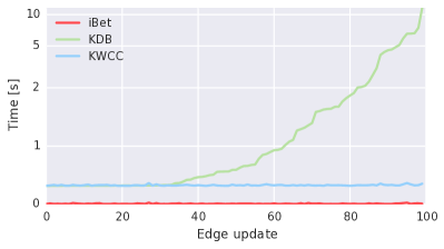
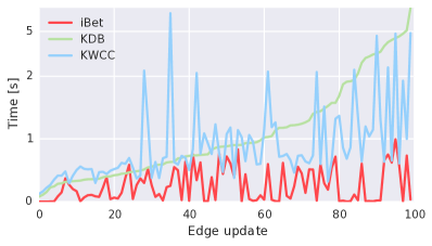
Figure 3. Running times of iBet, KDB and KWCC for 100 edge updates on oregon1-010526. Left: times for the APSP update step. Right: times for the dependency update step.

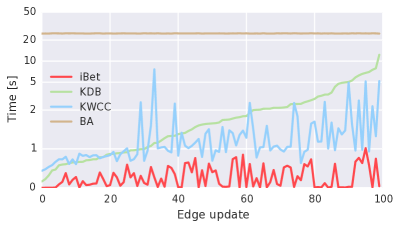
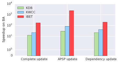
Figure 4. Left: Running times of iBet, KDB, KWCC and BA on the oregon1-010526 graph for 100 edge updates. Right: Average speedups on recomputation with BA (geometric mean) over all networks of Table 1 for the three incremental algorithms. The column on the left shows the speedup of the complete update, the one in the middle the speedup of the APSP update only and the one on the right the speedup of the dependency update only.

Figure 4 on the left reports the total running times of iBet, KDB, KWCC and BA on oregon1-010526. Although the running times vary significantly among the updates, iBet is always the fastest among all algorithms. On the contrary, there is not always a clear winner between KDB and KWCC. On the right, Figure 4 shows the geometric mean of the speedups on recomputation for the three incremental algorithms, considering the complete update, the APSP update step only and the dependency update step only, respectively. iBet is the method with the highest speedup both overall and on the APSP update and dependency update steps separately, meaning that each of the improvements described in Section 4.3 and Section 5.3 contribute to the final speedup. On average, iBet is a factor 82.7 faster than KDB and a factor 28.5 faster than KWCC on the APSP update step and it is a factor 9.4 faster than KDB and a factor 4.9 faster than KWCC on the dependency update step. Overall, the speedup of iBet on KDB ranges from 6.6 to 29.7 and is on average (geometric mean of the speedups) 14.7 times faster. The average speedup on KWCC is 7.4, ranging from a factor 4.1 to a factor 16.0.

8. Conclusions and future work

Computing betweenness centrality is a problem of great practical relevance. In this paper we have proposed and evaluated new techniques for the betweenness update after the insertion (or weight decrease) of an edge. Compared to other approaches, our new algorithm is easy to implement and significantly reduces the number of operations of both the APSP update and the dependency update. Our experiments on real-world networks show that our approach outperforms existing methods, on average approximately by one order of magnitude.

Future work might include parallelization for further acceleration. Furthermore, we plan to extend our techniques also to the decremental case (where an edge can be deleted from the graph or its weight can be increased) and to batch updates, where several edge updates might occur at the same time.

Although dynamic betweenness algorithms can be much faster than recomputation, a major limitation for their scalability is their memory requirement of $\Theta(n^{2})$. An interesting research direction is the design of scalable dynamic algorithms with a smaller memory footprint.

Our implementations are based on NetworKit [24], the open-source framework for network analysis, and we will publish our source code in upcoming releases of the package.

References

- [1] D. C. Bell, J. S. Atkinson, and J. W. Carlson. Centrality measures for disease transmission networks. Social Networks, 21(1):1–21, 1999.
- [2] E. Bergamini and H. Meyerhenke. Approximating betweenness centrality in fully dynamic networks. Internet Mathematics, 12(5):281–314, 2016.
- [3] E. Bergamini, H. Meyerhenke, and C. Staudt. Approximating betweenness centrality in large evolving networks. In 17th Workshop on Algorithm Enginnering and Experiments, ALENEX 2015, pages 133–146. SIAM, 2015.
- [4] P. Boldi and S. Vigna. Axioms for centrality. Internet Mathematics, 10(3-4):222–262, 2014.
- [5] M. Borassi and E. Natale. KADABRA is an adaptive algorithm for betweenness via random approximation. In 24th Annual European Symposium on Algorithms, ESA 2016, volume 57 of LIPIcs, pages 20:1–20:18. Schloss Dagstuhl - Leibniz-Zentrum fuer Informatik, 2016.
- [6] U. Brandes. A faster algorithm for betweenness centrality. Journal of Mathematical Sociology, 25:163–177, 2001.
- [7] P. Crescenzi, G. D’Angelo, L. Severini, and Y. Velaj. Greedily improving our own centrality in A network. In Experimental Algorithms - 14th International Symposium, SEA 2015, Proceedings, volume 9125 of Lecture Notes in Computer Science, pages 43–55. Springer, 2015.
- [8] R. Geisberger, P. Sanders, and D. Schultes. Better approximation of betweenness centrality. In 10th Workshop on Algorithm Engineering and Experiments (ALENEX ’08), pages 90–100. SIAM, 2008.
- [9] O. Green, R. McColl, and D. A. Bader. A fast algorithm for streaming betweenness centrality. In SocialCom/PASSAT, pages 11–20. IEEE, 2012.
- [10] T. Hayashi, T. Akiba, and Y. Yoshida. Fully dynamic betweenness centrality maintenance on massive networks. Proceedings of 41st International Conference on Very Large Data Bases (PVLDB 2015), 9(2):48–59, 2015.
- [11] M. Kas, M. Wachs, K. M. Carley, and L. R. Carley. Incremental algorithm for updating betweenness centrality in dynamically growing networks. In Advances in Social Networks Analysis and Mining 2013 (ASONAM ’13), pages 33–40. ACM, 2013.
- [12] C. Kiss and M. Bichler. Identification of influencers – measuring influence in customer networks. Decision Support Systems, 46(1):233 – 253, 2008.
- [13] D. Koschützki, K. A. Lehmann, L. Peeters, S. Richter, D. Tenfelde-Podehl, and O. Zlotowski. Centrality indices. In Network Analysis, volume 3418 of LNCS, pages 16–61. Springer Berlin Heidelberg, 2005.
- [14] N. Kourtellis, G. De Francisci Morales, and F. Bonchi. Scalable online betweenness centrality in evolving graphs. Knowledge and Data Engineering, IEEE Transactions on, PP(99):1–1, 2015.
- [15] J. Kunegis. KONECT: the koblenz network collection. In 22nd International World Wide Web Conference, WWW ’13, pages 1343–1350, 2013.
- [16] M. Lee, S. Choi, and C. Chung. Efficient algorithms for updating betweenness centrality in fully dynamic graphs. Information Sciences, 326:278–296, 2016.
- [17] J. Leskovec and A. Krevl. SNAP Datasets: Stanford large network dataset collection. http://snap.stanford.edu/data, June 2014.
- [18] C.-C. Lin and R.-C. Chang. On the dynamic shortest path problem. Journal of Information Processing, 13(4):470–476, Apr. 1991.
- [19] M. Nasre, M. Pontecorvi, and V. Ramachandran. Betweenness centrality - incremental and faster. In Mathematical Foundations of Computer Science 2014 - 39th International Symposium, MFCS 2014, volume 8635 of Lecture Notes in Computer Science, pages 577–588. Springer, 2014.
- [20] M. Pontecorvi and V. Ramachandran. Fully dynamic betweenness centrality. In Algorithms and Computation - 26th International Symposium, ISAAC 2015, Proceedings, volume 9472 of Lecture Notes in Computer Science, pages 331–342. Springer, 2015.
- [21] G. Ramalingam and T. W. Reps. On the computational complexity of dynamic graph problems. Theoretical Computer Science, 158(1&2):233–277, 1996.
- [22] M. Riondato and E. M. Kornaropoulos. Fast approximation of betweenness centrality through sampling. Data Mining and Knowledge Discovery, 30(2):438–475, 2016.
- [23] M. Riondato and E. Upfal. ABRA: approximating betweenness centrality in static and dynamic graphs with rademacher averages. In Proceedings of the 22nd ACM SIGKDD International Conference on Knowledge Discovery and Data Mining, 2016, pages 1145–1154. ACM, 2016.
- [24] C. L. Staudt, A. Sazonovs, and H. Meyerhenke. NetworKit: A tool suite for high-performance network analysis. Network Science, To appear.