Latest developments in the simulation of final states involving top-pair and heavy bosons

Abstract:

I give an overview of recent progress in the simulation of final states involving top-quarks and vector bosons pair. First I’ll discuss the recently found solutions needed to simulate fully differential top pair production ($pp\to b\bar{b}+4$ leptons) at NLO+PS accuracy, retaining off-shellness and interference effects exactly. In the second part, I’ll review the MiNLO (Multi-scale Improved NLO) method, and then show a recent application, namely the simultaneous NLO+PS description of $W^{+}W^{-}$ and $W^{+}W^{-}+1$ jet production.

In this article I will review a couple of recent results on the inclusion of higher-order QCD corrections to the Monte Carlo simulation of final states involving top-pair and heavy electroweak bosons. In section 1 I will focus on the recent progress achieved in the matching of QCD NLO corrections with parton shower simulations (NLO+PS) for the process $pp\to W^{+}W^{-}b\bar{b}$, whereas in section 2 I will discuss the NLO+PS merging of $W^{+}W^{-}$ and $W^{+}W^{-}$+1 jet production using the MiNLO method.

1 top-pair production

It is known that having an accurate simulation of the process $pp\to W^{+}W^{-}b\bar{b}$ is important for several reasons at the LHC, for instance to measure the top quark mass, or to have an unified treatment of $t\bar{t}$ and the so-called “single-top $Wt$” production.

At fixed order in QCD, $W^{+}W^{-}b\bar{b}$ hadronic production is very well known and much studied. Despite the fully differential cross section has been known for several years at NLO [1, 2, 3, 4, 5], with the exception of a first study appeared in [6], Monte Carlo NLO+PS event generators addressing all the issues related to the complete simulation of this final state started to be available only recently in the POWHEG approach [7, 8, 9]. In the rest of this section I’ll focus on these issues (and solutions thereof) within the POWHEG approach, although substantial work in this direction is also pursued within the MC@NLO matching scheme, and complete results for single-top t-channel production in the 4-flavour scheme were published in ref. [10].

The problem with the simulation of $W^{+}W^{-}b\bar{b}$ production and the inclusion of finite width effects can be stated as follows: unless special care is taken, the intermediate top-quark virtuality is not preserved among different parts of the computation, leading to the evaluation of matrix elements at phase space points which have different top virtualities. When this happens, three problems will in general occur:

1. at the level of computing NLO corrections with a subtraction method, the cancellation of collinear singularities associated to gluon emission off final-state $b$-quarks can become delicate, eventually failing when approaching the narrow-width limit.

2. when the hardest radiation is generated in POWHEG, the phase-space region associated to final-state gluon emission off the $b$-quark is handled by a mapping that, in general, does not preserve the virtuality of the intermediate resonance. Unless $m^{2}_{bg}\ll\Gamma_{t}E_{bg}$, real and Born matrix elements ($R$ and $B$, respectively) will not be on the resonance peak at the same time, hence the ratio $R/B$ in the POWHEG Sudakov can become large when $R$ is on peak and $B$ is not, yielding a spurious “Sudakov suppression”.

3. further problems can arise during the parton-showering stage: from the second emission onward, the shower should be instructed to preserve the mass of the resonances. This could be done easily if there was an unique mechanism to “assign” the radiation to a given resonance. For processes where interference(s) is(are) present, no obvious choice is possible.

An intermediate solution to the previous issues was presented in ref. [7], where a fully consistent NLO+PS simulation for $W^{+}W^{-}b\bar{b}$ production was obtained in the narrow-width limit, and off-shellenss and interference effects were implemented in an approximate way. I refer to the original paper, or to the review [11], for more details. Here it suffices to say that, by using the narrow-with approximation to compute NLO corrections, production and decay can be clearly separated (no interference arises), thereby allowing a non-ambiguous “resonance assignment” for final-state radiation, as well as the use of an improved (“resonance aware”) subtraction method, where radiation in the decay is generated by first boosting momenta in the resonance rest-frame. In this way, $B$ and $R$ are always evaluated with the same virtuality for the intermediate resonance, so that the subtraction can be safely performed, and no spurious Sudakov suppression can arise.

More recently, a general solution to include off-shellness and interference effects in the
POWHEG approach was proposed in ref. [8], and later applied to the $W^{+}W^{-}b\bar{b}$ process in ref. [9], where matrix elements were obtained using OpenLoops [12]. The main new concept introduced in [8] is that one separates all contributions to the cross section into terms with definite resonance structure, i.e. each term should only have peaks associated to a given resonance structure (“resonance history”). For $W^{+}W^{-}b\bar{b}$ production, for instance, one has two types of resonance histories: one where at least one $s$-channel top-propagator appears (this includes both doubly- and single-resonant contributions) and another associated to non-resonant production. By means of projectors $\Pi_{f_{b}}$ built by combining Breit-Wigner like functions $P^{f_{b}}$, a partition of the unit can be constructed, so that a given Born (and virtual) partonic subprocess $B$ can be separated into contributions $B_{f_{b}}$ that are, individually, dominated by one and only one resonance history (labeled by $f_{b}$):

$$B(\Phi_{B})=\sum_{f_{b}}B_{f_{b}}(\Phi_{B})\equiv\sum_{f_{b}}\Pi_{f_{b}}(\Phi_{B})B(\Phi_{B}),\ \ \mbox{where }\ \ \Pi_{f_{b}}(\Phi_{B})=\frac{P^{f_{b}}(\Phi_{B})}{\sum_{f^{\prime}_{b}}P^{f^{\prime}_{b}}(\Phi_{B})}\,.$$ (1)

Since each Born matrix element is separated according to resonance histories, one needs to set-up a similar mechanism for real matrix elements, such that, eventually, each projected real matrix element can be associated to an unique resonance history, with a counterpart in the corresponding list of Born’s ones. As usual, real matrix elements also need be separated according to their collinear singularities: to this end, one requires that a collinear region $\alpha_{r}$ is admitted only if the two collinear partons both arise either from the same resonance, or from the hard interaction. This separation is achieved schematically as

$$R=\sum_{\alpha_{r}}R_{\alpha_{r}},\ \ \mbox{where }\ \ R_{\alpha_{r}}=\frac{P^{f_{r}}d^{-1}(\alpha_{r})}{\sum_{f^{\prime}_{r}}(P^{f^{\prime}_{r}}\sum_{\alpha^{\prime}_{r}}d^{-1}(\alpha^{\prime}_{r}))}R\,.$$ (2)

In eq. (2), $f_{r}$ denotes a given resonance history assignment for $R$, $d(\alpha_{r})\to 0$ when the collinear region $\alpha_{r}$ is approached, and the sums in the denominator run only on the possible resonance histories $f^{\prime}_{r}$ present in $R$, and on the compatible singular regions $\alpha^{\prime}_{r}$ associated to a given $f^{\prime}_{r}$: hence a given $R_{\alpha_{r}}$ becomes dominant only if the collinear partons of region $\alpha_{r}$ have the smallest $k_{t}$ and the corresponding resonance history $f_{r}$ is the closest to its mass shell.

The above prescriptions allowed to build a POWHEG generator able to simulate processes with intermediate resonances, keeping all finite-width effects and interferences. In fact, having separated each contribution as explained above, for the singular regions associated to a radiation in a resonance decay, it becomes now possible to safely use the “resonance-aware” subtraction method developed in [7], thereby avoiding the mismatches mentioned at the beginning of this section. Similarly, because an index $\alpha_{r}$ is naturally associated to the hardest radiation generated by POWHEG, it’s possible to unambiguously assign the radiation to a given resonance, preventing the parton shower to distort the mass of the resonances.

The left panel of Fig. 1

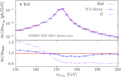
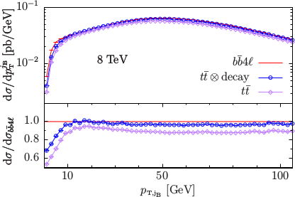
Figure 1: Invariant mass of the $W$ and hardest $b$-jet (left panel) and transverse momentum of the hardest $b$-jet (right panel), at the $\sqrt{S}=8$ TeV LHC. Figures taken from ref. [9].

shows the differences in shape of the reconstructed top peak obtained using three tools, namely the new generator of ref. [9] ($b\bar{b}4\ell$), the resonance-improved generator based on an approximate treatment of off-shell effects [7] ($t\bar{t}\,\otimes\,$decay), and the original generator [13] based on on-shell NLO matrix elements for $t\bar{t}$ production ($t\bar{t}$). As expected, the “$b\bar{b}4\ell$” and “$t\bar{t}\,\otimes\,$decay” generators are fairly consistent, especially close to the resonance peak, whereas the “$t\bar{t}$” generator shows larger deviations. The $p_{T}$ spectrum of the hardest $b$-jet is instead shown in the right panel of fig. 1, without imposing any particular cuts. The shape difference at small $p_{T}$ can be attributed to the fact that the “Wt” contribution is missing (approximate) in the “$t\bar{t}$” (“$t\bar{t}\,\otimes\,$decay”) generator, whereas it’s fully taken into account in the “$b\bar{b}4\ell$” one.

2 $W$-boson pair production

The study of vector boson pair-production is central for the LHC Physics program. Not only is $W^{+}W^{-}$ production measured to access anomalous gauge couplings, but it’s also an important background for several searches, notably for those where the $H\to W^{+}W^{-}$ decay is present. For these and other similar reasons, it is important to have flexible and fully realistic theoretical predictions that allow to simultaneously model, with high accuracy, the production of $W^{+}W^{-}$, inclusively as well as in presence of jets. The methods aiming at this task are usually referred to as “NLO+PS merging”. NLO+PS merging for $pp\to VV$+jet(s) was achieved using the MEPS@NLO [14, 15] and FxFx [16, 17] methods. In this section, I’ll review the MiNLO formalism and show how it was used to merge at NLO the processes $pp\to W^{+}W^{-}$ and $pp\to W^{+}W^{-}+$ jet [18].

The MiNLO (Multi-scale Improved NLO) procedure [19] was originally introduced as a prescription to a-priori choose the renormalization ($\mu_{R}$) and factorization ($\mu_{F}$) scales in multileg NLO computations: since these computations can probe kinematic regimes involving several different scales, the choice of $\mu_{R}$ and $\mu_{F}$ is indeed ambiguous, and the MiNLO method addresses this issue by consistently including CKKW-like corrections [20, 21] into a standard NLO computation. In practice this is achieved by associating a “most-probable” branching history to each kinematic configuration, through which it becomes possible to evaluate the couplings at the branching scales, as well as to include (MiNLO) Sudakov form factors (FF). This prescription regularizes the NLO computation also in the regions where jets become unresolved, hence the MiNLO procedure can be used within the POWHEG formalism to regulate the $\bar{B}$ function for processes involving jets at LO.

In a single equation, for a $q\bar{q}$-induced process as $W^{+}W^{-}$ production, the MiNLO-improved POWHEG $\bar{B}$ function reads:

$$\bar{B}_{\,\tt WWJ-MiNLO}=\alpha_{\scriptscriptstyle\rm S}(q_{T})\Delta^{2}_{q}(q_{T},M_{X})\Big{[}B(1-2\Delta^{(1)}_{q}(q_{T},M_{X}))+\alpha_{\scriptscriptstyle\rm S}V(\bar{\mu}_{R})+\alpha_{\scriptscriptstyle\rm S}\int d\Phi_{\mathrm{rad}}R\Big{]}\,,$$

where $X$ is the color-singlet system ($WW$ in this case), $q_{T}$ is its transverse momentum, $\bar{\mu}_{R}$ is set to $q_{T}$, and $\Delta_{q}(q_{T},Q)=\exp\Big{\{}-\int_{q^{2}_{T}}^{Q^{2}}\frac{dq^{2}}{q^{2}}\frac{\alpha_{\scriptscriptstyle\rm S}(q^{2})}{2\pi}\Big{[}A_{q}\log\frac{Q^{2}}{q^{2}}+B_{q}\Big{]}\Big{\}}$ is the MiNLO Sudakov FF associated to the jet present at LO. Convolutions with PDFs are understood, $B$ is the leading-order matrix element for the process $pp\to X+1$ jet (stripped off of the strong coupling), and $\Delta_{q}^{(1)}(q_{T},Q)$ (the $\mathcal{O}(\alpha_{\scriptscriptstyle\rm S})$ expansion of $\Delta_{q}$) is removed to avoid double counting. We also notice that $\bar{B}_{\,\tt WWJ-MiNLO}$ is a function of $\Phi_{X+j}$, i.e. the phase space to produce the $X$ system and an extra parton, which can be arbitrarily soft and/or collinear.

In ref. [22] it was also realized that, if $X$ is a color singlet, upon integration over the full phase space for the leading jet, one can formally recover NLO+PS accuracy for the process $pp\to X$ by properly applying MiNLO to NLO+PS simulations for processes of the type $pp\to X+1$ jet. Besides setting $\mu_{F}$ and $\mu_{R}$ equal to $q_{T}$ in all their occurrences, the key point is to include at least part of the Next-to-Next-to-Leading Logarithmic (NNLL) corrections into the MiNLO Sudakov form factor, namely the $B_{2}$ term: by omitting it, the full integral of eq. (2) over $\Phi_{X+j}$, albeit finite, differs from $\sigma_{pp\to X}^{NLO}$ by a relative amount $\alpha_{\scriptscriptstyle\rm S}(M_{X})^{3/2}$, thereby hampering a claim of NLO accuracy.

The $B_{2}$ coefficient is process-dependent, and formally also a function of $\Phi_{X}$, because part of it stems from the 1-loop correction to the $pp\to X$ process. For Higgs, Drell-Yan, and $VH$ production, these 1-loop corrections can be expressed as form factors: $B_{2}$ becomes just a number as its dependence upon $\Phi_{X}$ disappears, and the analogous of eq. (2) can be easily implemented [22, 24]. For diboson production, the situation is more delicate. First, extracting $B_{2}$ for the $WW$ case is more subtle, as the virtual corrections to the $pp\to WW$ process don’t factorize on the Born squared amplitude, hence $B_{2}=B_{2}(\Phi_{X})$. As a consequence, a mismatch between different phase spaces becomes apparent, because in eq. (2) $\bar{B}_{\,\tt WWJ-MiNLO}$ depends upon $\Phi_{X+j}$, whereas $B_{2}$ needs to be computed as a function of $\Phi_{X}$. In ref. [18] these two issues were handled as follows:

• to compute $B_{2}$ we started from the relatively simple expression used for the Drell-Yan case, and replaced its process-dependent part $[V/B]^{{\tt DY}}=C_{F}(\pi^{2}-8)$ with the corresponding term for $WW$ production: $[V/B]^{WW}(\Phi_{WW})=V^{WW}(\Phi_{WW})/B^{WW}(\Phi_{WW})$.

• in order to evaluate $B_{2}$, we defined on an event-by-event basis a projection of the $WW+1$ jet state onto a $WW$ one, using the FKS mapping relevant for initial-state radiation as implemented in the POWHEG BOX [25]. For real emission events, a similar mapping was used. In all cases, in the $q_{T}\to 0$ limit, the effect of these projections on the final state kinematics smoothly vanishes, making sure that the precise numerical determination of $B_{2}$ is affected only beyond the required accuracy.

In ref. [18] we have built a POWHEG generator for the $pp\to W^{+}W^{-}+1$ jet process, and upgraded it with MiNLO, according to the aforementioned procedure. We worked in the 4-flavour scheme, including exactly the vector bosons’ decay products, as well as finite-width effects and single-resonant contributions. Tree-level matrix elements were obtained with an interface to
MadGraph 4 [26, 27], whereas one loop corrections were computed with GoSam 2.0 [28, 24].

The left panel of Fig. 2

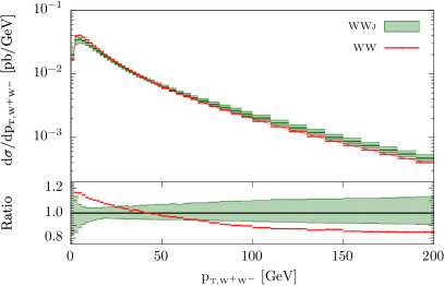
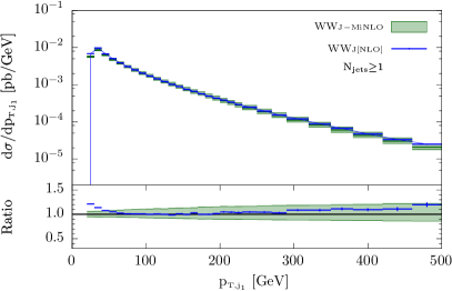
Figure 2: Transverse momenta of the $W^{+}W^{-}$ system (left panel) and of the leading jet (right panel), at the $\sqrt{S}=13$ TeV LHC. The green curve is the MiNLO prediction (central value with uncertainty) from ref. [18], the red one is obtained using the original POWHEG generator [29], and the blue line is a partonic NLO result. Figures taken from ref. [18].

shows the transverse momentum spectrum of the $WW$ system as obtained with the WWJ-MiNLO generator against the one obtained with the original POWHEG generator for $pp\to W^{+}W^{-}$ [29]. The importance of NLO corrections is manifest in the high-$p_{T}$ tail, whereas the differences at small $p_{T}$ can be attributed to the differences among the POWHEG and the MiNLO Sudakovs. The right panel shows instead a comparison for the leading jet $p_{T}$ spectrum between the parton-level computation $pp\to WW+1$ jet at NLO, and the MiNLO result. This observable is formally described with the same accuracy (NLO) by both predictions, as shown in the plot. The effect of resumming collinear logarithms at small $p_{T}$ is reflected in the difference between MiNLO and the pure NLO, where no resummation is included. At high $p_{T,j}$, the small differences are due to the fact that different central values for the $\mu_{R}$ and $\mu_{F}$ scales are used, namely $\mu=p_{T,WW}$ for MiNLO (as by prescription) and $\mu=m_{WW}$ at NLO.

It will be interesting to improve further the WWJ-MiNLO generator by including the effect of $gg$-induced contributions (an NLO+PS study for the $ZZ$ case was performed in ref. [30]) and, ultimately, matching it to the differential NNLO computation of ref. [31].

References

- [1] A. Denner, S. Dittmaier, S. Kallweit and S. Pozzorini, JHEP 1210, 110 (2012)
- [2] G. Bevilacqua, M. Czakon, A. van Hameren, C. G. Papadopoulos and M. Worek, JHEP 1102, 083 (2011)
- [3] G. Heinrich, A. Maier, R. Nisius, J. Schlenk and J. Winter, JHEP 1406, 158 (2014)
- [4] R. Frederix, Phys. Rev. Lett. 112, no. 8, 082002 (2014)
- [5] F. Cascioli, S. Kallweit, P. Maierhöfer and S. Pozzorini, Eur. Phys. J. C 74, no. 3, 2783 (2014)
- [6] M. V. Garzelli, A. Kardos and Z. Trocsanyi, JHEP 1408, 069 (2014)
- [7] J. M. Campbell, R. K. Ellis, P. Nason and E. Re, JHEP 1504, 114 (2015)
- [8] T. Ježo, and P. Nason, JHEP 1512, 065 (2015)
- [9] T. Ježo, J. M. Lindert, P. Nason, C. Oleari and S. Pozzorini, Eur. Phys. J. C 76, no. 12, 691 (2016)
- [10] R. Frederix, S. Frixione, A. S. Papanastasiou, S. Prestel and P. Torrielli, JHEP 1606, 027 (2016)
- [11] E. Re, PoS TOP 2015, 012 (2016)
- [12] F. Cascioli, P. Maierhöfer and S. Pozzorini, Phys. Rev. Lett. 108, 111601 (2012)
- [13] S. Frixione, P. Nason and G. Ridolfi, JHEP 0709, 126 (2007)
- [14] S. Höche, F. Krauss, M. Schonherr and F. Siegert, JHEP 1304, 027 (2013)
- [15] F. Cascioli, S. Höche, F. Krauss, P. Maierhöfer, S. Pozzorini and F. Siegert, JHEP 1401, 046 (2014)
- [16] R. Frederix and S. Frixione, JHEP 1212, 061 (2012)
- [17] J. Alwall et al., JHEP 1407, 079 (2014)
- [18] K. Hamilton, T. Melia, P. F. Monni, E. Re and G. Zanderighi, JHEP 1609, 057 (2016)
- [19] K. Hamilton, P. Nason and G. Zanderighi, JHEP 1210, 155 (2012)
- [20] S. Catani, F. Krauss, R. Kuhn and B. R. Webber, JHEP 0111, 063 (2001)
- [21] L. Lonnblad, JHEP 0205, 046 (2002)
- [22] K. Hamilton, P. Nason, C. Oleari and G. Zanderighi, JHEP 1305, 082 (2013)
- [23] R. Frederix and K. Hamilton, JHEP 1605, 042 (2016)
- [24] G. Luisoni, P. Nason, C. Oleari and F. Tramontano, JHEP 1310, 083 (2013)
- [25] S. Frixione, P. Nason and C. Oleari, JHEP 0711, 070 (2007)
- [26] J. Alwall et al., JHEP 0709, 028 (2007)
- [27] J. M. Campbell, R. K. Ellis, R. Frederix, P. Nason, C. Oleari and C. Williams, JHEP 1207, 092 (2012)
- [28] G. Cullen et al., Eur. Phys. J. C 74, no. 8, 3001 (2014)
- [29] T. Melia, P. Nason, R. Rontsch and G. Zanderighi, JHEP 1111, 078 (2011)
- [30] S. Alioli, F. Caola, G. Luisoni and R. Röntsch, Phys. Rev. D 95, no. 3, 034042 (2017)
- [31] M. Grazzini, S. Kallweit, S. Pozzorini, D. Rathlev and M. Wiesemann, JHEP 1608, 140 (2016)