Long-wavelength deformations and vibrational modes in empty and
liquid-filled microtubules and nanotubes: A theoretical study

Abstract

We propose a continuum model to predict long-wavelength vibrational modes of empty and liquid-filled tubules that are very hard to reproduce using the conventional force-constant matrix approach based on atomistic ab initio calculation. We derive simple quantitative expressions for long-wavelength longitudinal and torsional acoustic modes, flexural acoustic modes, as well as the radial breathing mode of empty or liquid-filled tubular structures that are based on continuum elasticity theory expressions for a thin elastic plate. We furthermore show that longitudinal and flexural acoustic modes of tubules are well described by those of an elastic beam resembling a nanowire. Our numerical results for biological microtubules and carbon nanotubes agree with available experimental data.

I Introduction

Tubular structures with diameters ranging from nanometers to meters abound in nature to fill various functions. The elastic response of most tubular structures is dominated by low-frequency flexural acoustic (ZA) modes. Much attention has been devoted to the nanometer-wide carbon nanotubes (CNTs) Jorio et al. (2008), which are extremely stiff Overney et al. (1993), and to their flexural modes Overney et al. (1993); Sazonova et al. (2004); Wang and Varadan (2006); Gibson et al. (2007). Correct description of soft flexural modes in stiff quasi-1D systems like nanotubes and nanowires is essential for calibrating nanoelectromechanical systems used for ultrasensitive mass detection and radio-frequency signal processing Roukes (2001); Sazonova et al. (2004). In CNTs and in related graphene nanoribbons, flexural ZA modes have also been shown to significantly influence the unsurpassed lattice thermal conductivity Majee and Aksamija (2016). Much softer microtubules formed of tubulin proteins, with a diameter $d{\approx}20$ nm, are key components of the cytoskeleton and help to maintain the shape of cells in organisms. In spite of their importance, there are only scarce experimental data available describing the elastic behavior of microtubules. The conventional approach to calculate the frequency spectrum is based on an atomistic calculation of the force-constant matrix. This approach often fails for long-wavelength acoustic modes, in particular the soft flexural ZA modes, due to an excessive demand on supercell size and basis convergence. Typical results of this shortcoming are numerical artifacts such as imaginary vibration frequencies Ling et al. (2010).

Here we offer an alternative way, based on continuum elasticity theory Love (1927) and its extension to planar Liu et al. (2016) and tubular structures Qian et al. (2007); Sirenko et al. (1996); Wang et al. (2006), to predict the frequency of acoustic modes in quasi-1D structures such as empty and liquid-filled tubes consisting of stiff graphitic carbon or soft tubulin proteins. While the scope of our approach is limited to long-wavelength acoustic modes, the accuracy of vibration frequencies calculated using the simple expressions we derive surpasses that of conventional atomistic ab initio calculations. Our approach covers longitudinal and torsional modes, flexural modes, as well as the radial breathing mode. We show that longitudinal and flexural acoustic modes of tubules are simply related to those of an elastic beam resembling a nanowire. Since the native environment of tubulin nanotubes contains water, we specifically consider the effect of a liquid on the vibrational modes of tubular structures. Our numerical results for tubulin microtubules and carbon nanotubes agree with available experimental data.

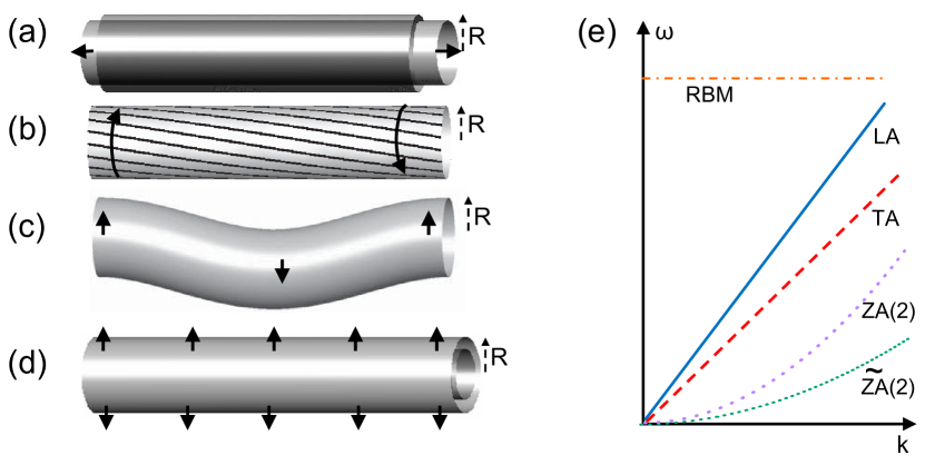
Figure 1: (Color online) Schematic representation of important deformations of a tubular structure. (a) Longitudinal acoustic (LA, stretching), (b) torsional acoustic (TA, torsion), (c) flexural acoustic (doubly degenerate ZA, bending), and (d) the radial breathing mode (RBM). (e) Schematic dispersion relations of the corresponding long-wavelength phonon modes. The tilde denotes liquid-filled tubules.

II Continuum elasticity approach

A 1D tubular structure of radius $R$ can be thought of as a rectangular 2D plate of width 2$\pi$R that is rolled up to a cylinder. Consequently, the elastic response of 1D tubules to strain, illustrated in Figs. 1(a)-1(d), is related to that of the constituting 2D plate. To describe this relationship in the linear regime and calculate the frequency of long-wavelength vibrational modes in 1D tubular structures, we take advantage of a continuum elasticity formalism that has been successfully adapted to 2D structures Liu et al. (2016).

As shown earlier Liu et al. (2016), elastic in-plane deformations of a plate of indefinite thickness may be described by the $(3{\times}3)$ 2D elastic stiffness matrix, which is given in Voigt notation by

$$\left(\begin{array}[]{ccc}c_{11}&c_{12}&0\\ c_{12}&c_{22}&0\\ 0&0&c_{66}\end{array}\right)\,.$$ (4)

Resistance of such a plate to bending is described by the flexural rigidity $D$. For a plate suspended in the $x-y$ plane, $c_{11}$ and $c_{22}$ describe the longitudinal strain-stress relationship along the $x-$ and $y-$direction, respectively. $c_{66}$ describes the elastic response to in-plane shear. For an isotropic plate, which we consider here, $c_{11}=c_{22}$, $c_{66}=(c_{11}-c_{12})/2$, and the in-plane Poisson ratio ${\alpha}=c_{12}/c_{11}$. Considering a 3D plate of finite thickness $h$, characterized by the $(6{\times}6)$ elastic stiffness matrix $C_{ij}$, the coefficients of the 2D elastic stiffness matrix $c_{ij}$ for the equivalent plate of indefinite thickness are related by $c_{ij}=h{\cdot}C_{ij}(1-\alpha_{\perp}^{2})$. This expression takes account of the fact that stretching a finite-thickness slab of isotropic material not only reduces its width by the in-plane Poisson ratio $\alpha$, but also its thickness by the out-of-plane Poisson ratio $\alpha_{\perp}$. This consideration is not needed for layered compounds such as graphite, where the inter-layer coupling is weak and $\alpha_{\perp}{\approx}0$, so that $c_{ij}=h{\cdot}C_{ij}$. In near-isotropic materials like tubulin, however, $\alpha_{\perp}{\approx}\alpha$ and $c_{ij}=h{\cdot}C_{ij}(1-\alpha^{2})$.

II.1 Vibrational Modes of empty Nanotubes

We now consider an infinitely thin 2D plate of finite width $2{\pi}R$ and an areal mass density $\rho_{2D}$ rolled up to a nanotube of radius $R$ that is aligned with the $x-$axis. The linear mass density of the nanotube is related to that of the plate by

$$\rho_{1D}=2{\pi}R\rho_{2D}\,.$$ (5)

In the long-wavelength limit, represented by $k=(2{\pi}/{\lambda}){\rightarrow}0$, the longitudinal acoustic mode of a tubular structure, depicted in Fig. 1(a), resembles the stretching mode of a 2D plate Liu et al. (2016). As mentioned above, the equivalent plate we consider here is a strip of finite width that is reduced during stretching due to the nonzero in-plane Poisson ratio $\alpha$.

In the following, we illustrate our computational approach for a tubular structure by focussing on its longitudinal acoustic mode. Our derivation, which is described in more detail in Appendices A and B, starts with the Lagrange function density

$$\mathcal{L}\left(\frac{du_{x}}{dx},\frac{du_{x}}{dt},x,t\right)=T-U$$

$$\quad=\frac{1}{2}\left[{\rho_{2D}}\left(\frac{du_{x}}{dt}\right)^{2}-c_{11}\left(1-\alpha^{2}\right)\left(\frac{du_{x}}{dx}\right)^{2}\right]2{\pi}R$$

$$\quad=\frac{1}{2}\left[\rho_{1D}\left(\frac{du_{x}}{dt}\right)^{2}-c_{LA}\left(\frac{du_{x}}{dx}\right)^{2}\right]\,,$$

where

$$c_{LA}=c_{11}\left(1-\alpha^{2}\right)2{\pi}R$$ (7)

is the longitudinal force constant of a 1D nanowire equivalent to the tubule, and the relation between $\rho_{1D}$ and $\rho_{2D}$ is defined in Eq. (5). The resulting Euler-Lagrange equation is

$$\frac{d}{dt}\left(\frac{{\partial}\mathcal{L}}{{\partial}\frac{du_{x}}{dt}}\right)+\frac{d}{dx}\left(\frac{{\partial}\mathcal{L}}{{\partial}\frac{du_{x}}{dx}}\right)=0\,.$$ (8)

Using the ansatz

$$u_{x}=u_{x,0}e^{i(kx-{\omega}t)}$$ (9)

we obtain the vibration frequency of the longitudinal acoustic (LA) mode of the nanotube or nanowire from

$$\omega_{LA}=\sqrt{\frac{c_{11}(1-\alpha^{2})}{\rho_{2D}}}~{}k=\sqrt{\frac{c_{LA}}{\rho_{1D}}}~{}k\,.$$ (10)

The prefactor of the crystal momentum $k$ is the longitudinal speed of sound. As already noted in Ref. [Lawler et al., 2006], the frequency of the LA mode is independent of the nanotube radius.

The torsional mode, depicted in Fig. 1(b), is very similar to the shear mode of a plate. Consequently, as shown in Appendix B, the vibration frequency of the torsional acoustic (TA) mode of the nanotube and the transverse acoustic mode of the plate should be the same. With $c_{66}$ describing the resistance of the equivalent plate to shear, we obtain

$$\omega_{TA}=\sqrt{\frac{c_{66}}{\rho_{2D}}}~{}k\,.$$ (11)

Again, prefactor of the crystal momentum $k$ is the corresponding speed of sound. Similar to the LA mode, the frequency of the TA mode is independent of the nanotube radius Lawler et al. (2006).

The doubly degenerate flexural acoustic (ZA) mode, depicted in Fig. 1(c), differs significantly from the corresponding bending mode of a plate Liu et al. (2016) that involves the plate’s flexural rigidity $D$. The continuum elasticity treatment of the bending deformation, described in Appendices A and B, leads to

$$\omega_{ZA} = \sqrt{\frac{{\pi}R^{3}c_{11}}{\rho_{1D}}\left(1+\frac{D}{c_{11}R^{2}}\right)}~{}k^{2}=\sqrt{\frac{D_{b}}{\rho_{1D}}}~{}k^{2}$$ (12)

$$= c_{ZA}(R)~{}k^{2}\,.$$

Here, $c_{ZA}$ is the effective bending force constant and $D_{b}$ is the effective beam rigidity of a corresponding nanowire, defined in Eq. (A16).

Finally, the radial breathing mode (RBM) of the nanotube, depicted Fig. 1(d), has a nearly $k-$independent frequency given by Liu et al. (2016)

$$\omega_{RBM}=\frac{1}{R}\sqrt{\frac{c_{11}}{\rho_{2D}}}\,.$$ (13)

The four vibration modes described above and their functional dependence on the momentum $k$ and radius $R$ have been partially described before using an elastic cylindrical shell model Sirenko et al. (1996); Wang et al. (2006). The schematic dependence of the vibration frequencies of these modes on $k$ is shown in Fig. 1(e). The main expressions for the vibration frequencies of both 2D and tubular 1D structures are summarized in Table 1.

II.2 Vibrational Modes of Liquid-Filled Nanotubes

We next consider the nanotubes completely filled with a compressible, but viscosity-free liquid that may slide without resistance along the nanotube wall Secchi et al. (2016). Since the nanotubes remain straight and essentially maintain their radius during stretching and torsion, the frequency $\tilde{\omega}$ of the LA and TA modes is not affected by the liquid inside, which remains immobile during the vibrations. We thus obtain

$$\tilde{\omega}_{LA}(k){\approx}\omega_{LA}(k)$$ (14)

and

$$\tilde{\omega}_{TA}(k)=\omega_{TA}(k)\,,$$ (15)

where the tilde refers to filling by a liquid.

The only effect of filling by a liquid on the flexural modes is an increase in the linear mass density to

$$\tilde{\rho}_{1D}=\rho_{1D}+{\pi}R^{2}\rho_{l}\,,$$ (16)

where $\rho_{l}$ denotes the gravimetric density of the liquid. In comparison to an empty tube, described by Eq. (12), we observe a softening of the flexural vibration frequency to

$$\tilde{\omega}_{ZA} = \sqrt{\frac{{\pi}R^{3}c_{11}}{\tilde{\rho}_{1D}}\left(1+\frac{D}{c_{11}R^{2}}\right)}~{}k^{2}=\sqrt{\frac{D_{b}}{\tilde{\rho}_{1D}}}~{}k^{2}$$ (17)

$$= \tilde{c}_{ZA}(R)~{}k^{2}\,.$$

Finally, as we expand in Appendix C, the effect of the contained liquid on the RBM frequency will depend on the stiffness of the tubular container. For stiff carbon nanotubes, the RBM mode is nearly unaffected, whereas the presence of an incompressible liquid increases $\tilde{\omega}_{RBM}$ in soft tubules. Thus,

$$\tilde{\omega}_{RBM}{\gtrsim}\omega_{RBM}\,.$$ (18)

The schematic dependence of the four vibration modes on the momentum $k$ in liquid-filled nanotubes is shown in Fig. 1(e). The main expressions for the vibration frequencies of liquid-filled tubular 1D structures are summarized in Table 1.

Table 1: Summary of expressions derived for the vibrational frequencies $\omega$ of 1D tubules and 2D plates. $\tilde{\omega}$ denotes the frequency of liquid-filled tubules. Equation numbers refer to the present publication.

Mode	1D Tubules	Equation	2D Plates
LA	$\omega_{LA}=\sqrt{\frac{c_{11}(1-\alpha^{2})}{\rho_{2D}}}~{}k$	Eq. (10)	$\omega_{LA}=\sqrt{\frac{c_{11}}{\rho_{2D}}}~{}k$
	$\omega_{LA}=\sqrt{\frac{c_{LA}}{\rho_{1D}}}~{}k$	Eq. (10)
	$\tilde{\omega}_{LA}=\omega_{LA}$
TA	$\omega_{TA}=\sqrt{\frac{c_{66}}{\rho_{2D}}}~{}k$	Eq. (11)	$\omega_{TA}=\sqrt{\frac{c_{66}}{\rho_{2D}}}~{}k$
	$\tilde{\omega}_{TA}=\omega_{TA}$
ZA	$\omega_{ZA}=$
	$\quad\sqrt{\frac{{\pi}R^{3}c_{11}}{\rho_{1D}}\left(1+\frac{D}{c_{11}R^{2}}\right)}~{}k^{2}$	Eq. (12)	$\omega_{ZA}=\sqrt{\frac{D}{\rho_{2D}}}$
	$\omega_{ZA}=\sqrt{\frac{D_{b}}{\rho_{1D}}}~{}k^{2}$	Eq. (12)
	$\tilde{\omega}_{ZA}=$
	$\quad\sqrt{\frac{{\pi}R^{3}c_{11}}{\tilde{\rho}_{1D}}\left(1+\frac{D}{c_{11}R^{2}}\right)}~{}k^{2}$	Eq. (17)
	$\tilde{\omega}_{ZA}=\sqrt{\frac{D_{b}}{\tilde{\rho}_{1D}}}~{}k^{2}$	Eq. (17)
RBM	$\omega_{RBM}=\frac{1}{R}\sqrt{\frac{c_{11}}{\rho_{2D}}}$	Eq. (13)
	$\tilde{\omega}_{RBM}{\gtrsim}\omega_{RBM}$	Eq. (18)

III Vibrational Modes of Nanotubes in a Surrounding Liquid

From among the four long-wavelength vibrational modes of nanotubes illustrated in the left panels of Fig. 1, the stretching and the torsional modes are not affected by the presence of a liquid surrounding the nanotube. We expect the radial breathing mode in Fig. 1(d) to couple weakly and be softened by a small amount in the immersing liquid. The most important effect of the surrounding liquid is expected to occur for the flexural mode shown in Fig. 1(c).

The following arguments and expressions have been developed primarily to accommodate soft biological structures such as tubulin-based microtubules, which require an aqueous environment for their function. We will describe the surrounding liquid by its gravimetric density $\rho_{l}$ and viscosity $\eta$. As suggested above, we will focus our concern on the flexural long-wavelength vibrations of such structures.

As we will show later on, the flexural modes of idealized, free-standing biological microtubules are extremely soft. In that case, the velocity of transverse vibrations will also be very small and definitely lower than the speed of sound in the surrounding liquid. Under these conditions, the motion of the rod-like tubular structure will only couple to the evanescent sound waves in the surrounding liquid and there will be no radiation causing damping. The main effect of the immersion in the liquid will be to increase the effective inertia of the rod. We may assume that the linear mass density $\rho_{1D}$ of the tubule in vacuum may increase to $\tilde{\rho}_{1D}=\rho_{1D}+{\Delta}\rho_{1D}$ in the surrounding liquid. We can estimate ${\Delta}\rho_{1D}={\Delta}A\rho_{l}$, where ${\Delta}A$ describes the increase in the effective cross-section area of the tubule due to the surrounding liquid that is dragged along during vibrations. We expect ${\Delta}A{\lesssim}{\pi}R^{2}$, where $R$ is the radius of the tubule. The softening of the flexural mode frequency $\tilde{\omega}_{ZA}$ due to the increase in $\rho_{1D}$ is described in Eq. (17).

Next we consider the effect of viscosity of the surrounding liquid on long-wavelength vibrations of a tubular structure that will resemble a rigid rod for $k{\rightarrow}0$. Since – due to Stoke’s paradox – there is no closed expression for the drag force acting on a rod moving through a viscous liquid, we will approximate the rod by a rigid chain of spheres of the same radius, which are coupled to a rigid substrate by a spring. The motion for a rigid chain of spheres is the same as of a single sphere, which is damped by the drag force $F=6{\pi}{\eta}Rv$ according to Stoke’s law, where $v$ is the velocity.

The damped harmonic motion of a sphere of radius $R$ and mass $m$ is described by

$$m\frac{d^{2}{u}}{dt^{2}}=-m{\omega_{0}^{2}}u-6{\pi}{\eta}R\frac{du}{dt}\,.$$ (19)

With the ansatz $u(t)=u_{0}e^{i{\omega}t}$, we get

$$-m\omega^{2}=-m\omega_{0}^{2}-i{\omega}6{\pi}{\eta}R$$ (20)

and thus

$$\omega=\pm\sqrt{\omega_{0}^{2}-\left(\frac{3{\pi}{\eta}R}{m}\right)^{2}}+i\frac{3{\pi}{\eta}R}{m}\,.$$ (21)

Assuming that the damping is small, we can estimate the energy loss described by the $Q-$factor

$$Q=\omega_{0}\frac{m}{3{\pi}{\eta}R}=\frac{2}{3}\frac{m}{R}\frac{f_{0}}{\eta}\,,$$ (22)

where $f_{0}=\omega_{0}/(2{\pi})$ is the harmonic vibration frequency. In a rigid string of masses separated by the distance $2R$, the linear mass density is related to the individual masses by $\rho_{1D}=m/(2R)$. Then, the estimated value of the $Q-$factor will be

$$Q=\frac{4}{3}\rho_{1D}\frac{f_{0}}{\eta}\,.$$ (23)

IV Computational Approach to Determine the Elastic Response of Carbon Nanotubes

We determine the elastic response and elastic constants of an atomically thin graphene monolayer, the constituent of CNTs, using ab initio density functional theory (DFT) as implemented in the SIESTA Artacho et al. (2008) code. We use the Perdew-Burke-Ernzerhof (PBE) Perdew et al. (1996) exchange-correlation functional, norm-conserving Troullier-Martins pseudopotentials Troullier and Martins (1991), and a double-$\zeta$ basis including polarization orbitals. To determine the energy cost associated with in-plane distortions, we sampled the Brillouin zone of a 3D superlattice of non-interacting layers by a $20{\times}20{\times}1$ $k$-point grid Monkhorst and Pack (1976). We used a mesh cutoff energy of $180$ Ry and an energy shift of 10 meV in our self-consistent total energy calculations, which has provided us with a precision in the total energy of ${\leq}2$ meV/atom. The same static approach can be applied to other layered materials that form tubular structures.

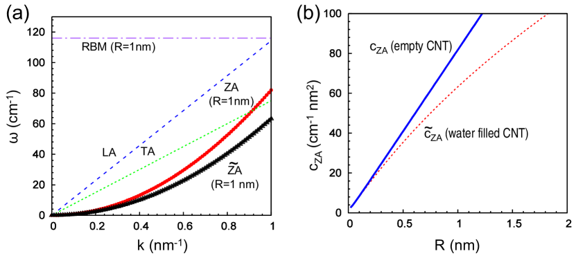
Figure 2: (Color online) (a) Frequency of vibrational modes depicted in Fig. 1(a) in empty and water-filled carbon nanotubes. (b) Dependence of the flexural coefficient $c_{ZA}(R)$, defined in Eq. (12), on the radius $R$ of empty and water-filled carbon nanotubes. The tilde denotes liquid-filled nanotubes.

V Results

To illustrate the usefulness of our approach for all tubular structures, we selected two extreme examples. Nanometer-wide CNTs have been characterized well as rigid structures able to support themselves in vacuum. Tubulin-based microtubules, on the other hand, are significantly wider and softer than carbon nanotubes. These biological structures require an aqueous environment for their function.

V.1 Carbon Nanotubes

Table 2: Elastic behavior of a 2D graphene monolayer. $c_{11}$, $c_{22}$, $c_{66}$ are 2D elastic stiffness constants defined in Eq. (4). $\alpha$ is the in-plane Poisson ratio, $D$ is the flexural rigidity, and $\rho_{2D}$ is the areal mass density. These values can be used directly to calculate long-wavelength acoustic frequencies $\omega(k)$ using the expressions in Table 1 and the speed of sound $v_{LA}$ and $v_{TA}$. Present values are compared to published data.

Quantity	Present result	Literature values
$c_{11}=c_{22}$	352.6 N/m	342 N/m
$c_{66}$	146.5 N/m	144 N/m a
$\alpha$	0.17	0.19 a
$D$	$0.22$ GPa${\cdot}$nm3	$0.225$ GPa${\cdot}$nm3
$R~{}\omega_{RBM}=\sqrt{c_{11}/\rho_{2D}}$	$116$ cm-1nm	$116$ cm-1nm
		$108$ cm-1nm
$v_{LA}$	21.5 km/s	22 km/s  a
		${\approx}21$ km/s
$v_{TA}$	14.1 km/s	14 km/s a,b

The elastic behavior of carbon nanotubes can be described using quantities previously obtained using DFT calculations for graphene Liu et al. (2016). The calculated elements of the elastic stiffness matrix (4) are $c_{11}=c_{22}=352.6$ N/m, $c_{12}=59.6$ N/m, and $c_{66}=146.5N/m$, all in very good agreement with experimental results Politano et al. (2012). The calculated in-plane Poisson ratio $\alpha=c_{12}/c_{11}=0.17$ is also close to the experimentally estimated value for graphene Politano et al. (2012) of $\alpha_{expt}=0.19$. The calculated flexural rigidity of a graphene plate is $D=0.22$ GPa$\cdot$nm³. The calculated 2D mass density of graphene $\rho_{2D}=0.743{\cdot}10^{-6}$ kg/m² translates to $\rho_{1D}=0.743{\cdot}10^{-6}$ kg/m²${\cdot}2{\pi}R$ for nanotubes of radius $R$.

The phonon dispersion relations ${\omega}(k)$ depend primarily on the radius and not the specific chiral index $(n,m)$ of carbon nanotubes and are presented in Fig. 2(a) for the different polarizations. The LA and TA mode frequencies are almost independent of the nanotube radius for a given $k$. The corresponding group velocities at $k{\to}0$ give the longitudinal speed of sound of $v_{LA}=d{\omega}_{LA}/dk=21.5$ km/s and the speed of sound with torsional polarization of $v_{TA}=d{\omega}_{TA}/dk=14.1$ km/s.

The flexural or bending ZA mode does depend on the nanotube radius through the proportionality constant $c_{ZA}(R)$, defined in Eq. (12), which is plotted as a function of $R$ in Fig. 2(b). The dispersion of the ZA mode in a CNT of radius $R=1$ nm is shown in Fig. 2(a). Also the RBM frequency depends on the nanotube radius according to Eq. (13). We find the value $\sqrt{c_{11}/\rho_{2D}}=116$ cm^-1nm of the prefactor of $R^{-1}$ in Eq. (13) to agree well with the published theoretical value Sánchez-Portal et al. (1999) of $116$ cm^-1nm and with the value of $108$ cm^-1nm, obtained by fitting a set of observed Raman frequencies Maultzsch et al. (2005). The calculated value ${\omega}_{RBM}=116$ cm^-1 for CNTs with $R=1$ nm is shown in Fig. 2(a).

Filling the CNT with a liquid of density $\rho_{l}$ increases its linear density $\rho_{1D}$ according to Eq. (16). For a nanotube filled with water of density $\rho_{l}=1$ g/cm³, the radius-dependent quantity $\tilde{c}_{ZA}(R)$, defined in Eq. (17), is plotted as a function of $R$ in Fig. 2(b). The dispersion of the $\tilde{\rm{ZA}}$ mode in a water-filled CNT of radius $R=1$ nm is shown in Fig. 2(a).

Elastic constants calculated in this work, and results derived using the present continuum elasticity approach are listed and compared to literature data in Table 2.

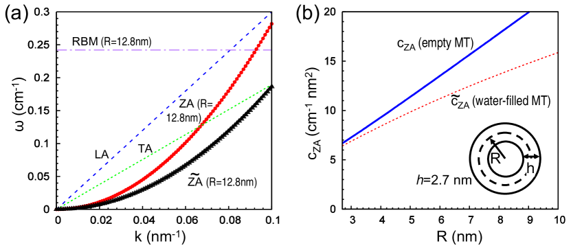
Figure 3: (Color online) (a) Frequency of vibrational modes depicted in Fig. 1(a) in empty and water-filled tubulin-based microtubules. (b) Dependence of the flexural coefficient $c_{ZA}(R)$, defined in Eq. (12), on the radius $R$ of empty and water-filled tubulin-based microtubules. The tilde denotes liquid-filled tubules.

V.2 Tubulin-Based Microtubules

To describe phonon modes in tubulin-based microtubules, we depend on published experimental data Venier et al. (1994) for microtubules with an average radius $R=12.8$ nm and a wall thickness $h=2.7$ nm. The observed density of the tubule wall material ${\rho}=1.47$ g/cm³ translates to ${\rho}_{2D}=4.0{\cdot}10^{-6}$ kg/m². The estimated Young’s modulus of the wall material is $E=0.5$ GPa and the flexural beam rigidity of these microtubules with $R=12.8$ nm is $D_{b}=0.9{\cdot}10^{-23}$ $N{\cdot}m^{2}$. We may use the relationship between $D_{b}$ and $D$, defined in Eq. (A15), to map these values onto the elastic 2D wall material and obtain $c_{11}=E{\cdot}h=1.4$ N/m and $D=2.71$ GPa$\cdot$nm³. In a rough approximation, tubulin can be considered to be isotropic, with a Poisson ratio ${\alpha}=0.25$. Further assuming that $c_{11}=c_{22}$, we estimate $c_{66}=(c_{11}-c_{12})/2=c_{11}(1-{\alpha})/2=0.5$ N/m.

One fundamental difference between tubulin-based microtubules and systems such as CNTs is that the former necessitate an aqueous environment for their shape and function. Thus, the correct description of microtubule deformations and vibrations requires addressing the complete microtubule-liquid system, which would exceed the scope of this study. We rather resorted to the expressions derived in the Subsection on nanotubes in a surrounding liquid to at least estimate their $Q-$factor in an aqueous environment. We used $\rho_{1D}=7{\times}10^{-13}$ kg/m for a water-filled microtubule, $\eta=10^{-3}$ Pa$\cdot$s and $f_{0}=10^{9}$ Hz, which provided us with the value $Q{\approx}1.2$. In other words, flexural vibrations in microtubules should be highly damped in aqueous environment, so their frequency should be very hard to measure. Consequently, the only available comparison between our calculations and experimental data should be made for static measurements.

An elegant way to experimentally determine the effective beam rigidity of individual tubulin-based microtubules involves the measurement of buckling caused by applying an axial buckling force using optical tweezers. Experimental results for the effective beam rigidity have been obtained in this way for microtubules that are free of the paclitaxel stabilizing agent and contain 14 tubulin protofilaments, which translates to the effective radius $R{\approx}9.75$ nm. The observed values range from $D_{b}=3.7{\pm}0.8{\times}10^{-24}$ Nm² Felgner et al. (1996) to $D_{b}=7.9{\pm}0.7{\times}10^{-24}$ Nm² Kikumoto et al. (2006), in good agreement with our calculated value $D_{b}=4.2{\times}10^{-24}$ Nm². Our estimated value $D_{b}=6.2{\times}10^{-24}$ Nm² for wider tubules with 16 protofilaments is 49% larger than for the narrower tubules with 14 protofilaments. The corresponding increase by 49% has been confirmed in a corresponding experiment Kikumoto et al. (2006).

Next, we may still use the oversimplifying assumption that tubulin microtubules may exist in the vacuum and could be described by the above-derived continuum values Wang et al. (2006). In this way, we may compare our results to published theoretical results. The calculated phonon dispersion relations ${\omega}(k)$ for most common microtubules with the radius $R=12.8$ nm are presented in Fig. 3(a). The LA and TA mode frequencies are independent of the tubule radius. From their slope, we get the longitudinal speed of sound $v_{LA}=d{\omega}_{LA}/dk=0.56$ km/s and the speed of sound with torsional polarization $v_{TA}=d{\omega}_{TA}/dk=0.36$ km/s. For the sake of comparison, we extracted the $v_{LA}$ value based on the elastic cylindrical shells model with $E=2.0$ GPa from Ref. Wang et al. (2006). Extrapolating to the value $E=0.5$ GPa in our set of parameters using the relationship $v_{LA}{\propto}\sqrt{E}$, we obtained $v_{LA}=0.59$ km/s, in excellent agreement with our calculated value.

The flexural or bending ZA mode depends on the tubule radius through the proportionality constant $c_{ZA}(R)$, defined in Eq. (12), which is plotted as a function of $R$ in Fig. 3(b). The dispersion of the ZA mode in a microtubule of radius $R=12.8$ nm is shown in Fig. 3(a).

Also the RBM frequency depends on the nanotube radius according to Eq. (13). For $R=12.8$ nm, we obtain ${\omega}_{RBM}=0.24$ cm^-1, as seen in Fig. 3(a).

To describe the increase in the linear density $\rho_{1D}$ of a microtubule filled with a liquid of density $\rho_{l}$, we have to account for the finite thickness $h$ of the wall and replace the radius $R$ by $R-h/2$ in Eq. (16). Considering water of density $\rho_{l}=1$ g/cm³ as the filling medium, we plot the radius-dependent quantity $\tilde{c}_{ZA}(R)$, defined in Eq. (17), as a function of $R$ in Fig. 3(b). The dispersion of the $\tilde{\rm{ZA}}$ mode in a water-filled CNT of radius $R=12.8$ nm is shown in Fig. 3(a).

Our results in Fig. 3(a) suggest soft vibration in the GHz range, in agreement with other theoretical estimates Sirenko et al. (1996); Wang et al. (2006). As mentioned above, all these vibrations will be hight damped in an aqueous environment to the low $Q-$factor.

VI Discussion

Our study has been motivated by the fact that the conventional approach to calculate the frequency spectrum, based on an atomistic calculation of the force-constant matrix, does not provide accurate frequencies for long-wavelength soft acoustic modes in quasi-1D tubular structures. We should note that the atomistic approach is quite adequate to determine frequencies of the optical and of short-wavelength acoustic modes. But for long-wavelength acoustic modes, the excessive demand on supercell size and basis convergence often yields imaginary vibration frequencies as an artifact of insufficient convergence.

As a viable alternative to tedious atomistic calculations of the force-constant matrix of complex tubular systems, we propose here a continuum elasticity approach to determine the frequency of long-wavelength acoustic modes in tubular structures that does not require the thickness of the wall as an input. Our approach for quasi-1D structures is based on the successful description of corresponding modes in 2D structures Liu et al. (2016). The continuum elasticity approach introduced in this study has a significant advantage over the 3D elastic modulus approach, which which has lead to inconsistencies in describing the elastic behavior of thin walls and membranes Wu et al. (1985). Using this approach, we obtain for the first time quantitative results for systems ranging from stiff CNTs to much wider and softer protein microtubules.

We found that the elastic behavior of the wall material can be determined accurately by static calculations of 2D plate subjected to small deformation or by elastic measurements. The validity of predictions based on this approach is limited to long-wavelength vibrations and large-radius nanotubes, both of which would require extraordinary computational resources in atomistic calculations. In particular, the flexural ZA modes with their ${\omega}{\propto}k^{2}$ momentum dependence are known to be very hard to reproduce by ab initio calculations near the $\Gamma$ point Ling et al. (2010).

For the sake of completeness, we have also derived the Euler-Lagrange equations of motion required to describe all long-wavelength acoustic modes and present the detailed derivation in the Appendix.

Of course, the frequency of the ZA modes is expected to be much softer than that of the LA mode in any nanotube or nanowire. Since ${\omega}_{ZA}{\propto}k^{2}$ whereas ${\omega}_{LA}{\propto}k$, expressions derived here for the long-wavelength limit would lead to the unrealistic behavior ${\omega}_{ZA}>{\omega}_{LA}$ for large values of $k$. This limits the $k-$range, for which our formalism is valid in the dispersion relations presented in Figs. 2(a) and 3(a). In a crystalline tubule, $k$ is restricted to typically an even smaller range given by the size of the 1D Brillouin zone.

For systems with a vanishing Poisson ratio $\alpha$, the radial breathing mode (RBM) should be decoupled from the longitudinal acoustic or stretching mode. However, as discussed in Appendix D, most systems have a non-vanishing value of $\alpha$. In that case, the two modes mix and change their character beyond the wavevector $k=1/R$, where ${\omega}_{LA}(k){\approx}{\omega}_{RBM}$, as discussed previously Wang et al. (2006). At smaller values of $k$, coupling between the LA mode and the RBM modifies the frequency of these modes by only ${\approx}1$% in CNTs.

Our model allows a simple extension from empty to liquid-filled nanotubes. We find that presence of a filling liquid does not affect longitudinal acoustic and torsional acoustic modes to a significant extent, as shown in Appendix C, but softens the flexural modes. We also expect the pressure wave of the liquid to couple to the RBM beyond the wavevector $k{\approx}{\omega}_{RBM}/v_{p}$, where $v_{p}$ is the speed of the propagating pressure wave.

To demonstrate the universality of our approach, we also considered microtubules formed of the proteins $\alpha$- and $\beta$-tubulin. These are responsible for maintaining the shape and elasticity of cells, but are too complex for an atomistic description to predict vibration spectra. From a computational point of view, the necessity to include the aqueous environment in the description of tubulin-based microtubules adds another layer of complexity to the problem.

Our basic finding that microtubule motion and vibrations are overdamped in the natural aqueous environment, with a $Q-$factor of the order of unity, naturally explains the absence of experimental data reporting observation of motion, dynamical shape changes and vibrations in these protein-based systems. Among static measurements of the elastic behavior of microtubules, optical tweezers appear to be the optimum way to handle and deform individual microtubules in order to determine their effective beam rigidity $D_{b}$. In this static scenario, we find our description of the beam rigidity precise enough to compare with experimental data. The reported dependence of $D_{b}$ on the cube of the radius Kikumoto et al. (2006) is reflected in our corresponding expression for $D_{b}$ in Eq. (A15). In the case of tubulin-based microtubules, we find the leading term in $D_{b}$ to be indeed proportional to $R^{3}$ and to be much larger than the second term, which is proportional to $R$.

VII Summary and Conclusions

Addressing the shortcoming of conventional atomistic calculations of long-wavelength acoustic frequencies in tubular structures, which often yield numerical artifacts, we have developed an alternative computational approach representing an adaptation of continuum elasticity theory to 2D and 1D structures. Since 1D tubular structures can be viewed as 2D plates of finite width rolled up to a cylinder, we have taken advantage of the correspondence between 1D and 2D structures to determine their elastic response to strain. In our approach, computation of long-wavelength acoustic frequencies does not require the determination and diagonalization of a large, momentum-dependent dynamical matrix. Instead, the simple expressions we have derived for the acoustic frequencies $\omega(k)$ use only four elements of a $k-$independent 2D elastic matrix, namely $c_{11}$, $c_{22}$, $c_{12}$, and $c_{66}$, as well as the value of the flexural rigidity $D$ of the 2D plate constituting the wall. These five numerical values can easily be obtained using static calculations for a 2D plate. Even though the scope of our approach is limited to long-wavelength acoustic modes, we found that the accuracy of the calculated vibration frequencies surpasses that of conventional atomistic ab initio calculations. Starting with a Lagrange function describing longitudinal, torsional, flexural and radial deformations of empty or liquid-filled tubular structures, we have derived corresponding Euler-Lagrange equations to obtain simple expressions for the vibration frequencies of the corresponding modes. We have furthermore shown that longitudinal and flexural acoustic modes of tubules are well described by those of an elastic beam resembling a nanowire. Using our simple expressions, we were able to show that a pressure wave in the liquid contained in a stiff carbon nanotube has little effect on its RBM frequency, whereas the effect of a contained liquid on the RBM frequency in much softer tubulin tubules is significant. We found that presence of water in the native environment of tubulin microtubules reduces the $Q-$factor to such a degree that flexural vibrations can hardly be observed. We also showed that the coupling between long-wavelength LA modes and the RBM can be neglected. We have found general agreement between our numerical results for biological microtubules and carbon nanotubes and available experimental data.

VIII Appendix

Material in the Appendix provides detailed derivation of expressions used in the main text and considers specific limiting cases. In Appendix A, we derive the Lagrange function for stretching, torsional and bending modes of tubular structure. In Appendix B, we derive analytical expressions for the frequencies of the corresponding vibration modes using the Euler-Lagrange equations. The effect of a liquid contained inside a CNT on its RBM frequency is investigated in Appendix C. The coupling between the longitudinal acoustic mode and the RBM in a CNT due to its non-vanishing Poisson ratio is discussed in Appendix D.

A A. Lagrange Function of a Strained Nanotube

A.1 Stretching

Let us consider a nanotube of radius $R$ aligned with the $x-$axis and its response to tensile strain ${du_{x}}/{dx}$ applied uniformly along the $x-$direction. The strain energy will be the same as that of a 2D strip of width $y=2{\pi}R$ lying in the $xy-$plane that is subject to the same condition.

Assuming that the width of the strip is constrained to be constant, the strain energy per length is given by

$$U_{x}=\frac{1}{2}~{}c_{11}\left(\frac{du_{x}}{dx}\right)^{2}2\pi R\,.$$ (A1)

For a nonzero Poisson ratio $\alpha$, stretching the strip by $du_{x}/dx$ will reduce its width by $du_{y}/dy={\alpha}du_{x}/dx$ and its radius $R$, as shown in Fig. 1(a). Releasing the constrained width will release the energy $U_{y}=-{\alpha}^{2}U_{x}$. The total strain energy per length of a nanotubule or an equivalent 1D nanowire is the sum $U=U_{x}+U_{y}$ and is given by

$$U = \frac{1}{2}c_{11}\left(1-\alpha^{2}\right)\left(\frac{du_{x}}{dx}\right)^{2}2\pi R$$ (A2)

$$= \frac{1}{2}c_{LA}\left(\frac{du_{x}}{dx}\right)^{2}\,.$$

Here, $c_{LA}=2{\pi}Rc_{11}(1-\alpha^{2})$ is the the longitudinal force constant of a 1D nanowire equivalent to the tubule, defined in Eq. (7).

In the harmonic regime, we will consider only small strain values. Releasing the strain will cause a vibration in the $x$-direction with the velocity $v_{x}=du_{x}/dt$. Then, the kinetic energy density of the strip will be given by

$$T=\frac{1}{2}{\rho_{2D}}\left(\frac{du_{x}}{dt}\right)^{2}2\pi R=\frac{1}{2}{\rho_{1D}}\left(\frac{du_{x}}{dt}\right)^{2}\,,$$ (A3)

where ${\rho_{2D}}$ is the areal mass density of the equivalent strip that is related to ${\rho_{1D}}$ by Eq. (5). The Lagrangian density is then given by

$$\mathcal{L}\left(\frac{du_{x}}{dx},\frac{du_{x}}{dt},x,t\right)=T-U$$ (A4)

$$\quad=\frac{1}{2}\left[{\rho_{2D}}\left(\frac{du_{x}}{dt}\right)^{2}-c_{11}\left(1-\alpha^{2}\right)\left(\frac{du_{x}}{dx}\right)^{2}\right]2{\pi}R\,,$$

$$\quad=\frac{1}{2}\left[\rho_{1D}\left(\frac{du_{x}}{dt}\right)^{2}-c_{LA}\left(\frac{du_{x}}{dx}\right)^{2}\right]\,.$$

A.2 Torsion

The derivation of the Euler-Lagrange equation for the torsional motion is very similar to that for the longitudinal motion. The main difference is that the displacement $u_{\phi}$ is normal to the propagation direction $x$. To obtain the corresponding equations, we need to replace $u_{x}$ by $u_{\phi}$ and $c_{11}(1-\alpha^{2})$ by $c_{66}$ in Eqs. (A1)-(A4). The Lagrangian density is then given by

$$\mathcal{L}\left(\frac{du_{\phi}}{dx},\frac{du_{\phi}}{dt},x,t\right)=T-U$$ (A5)

$$\quad=\frac{1}{2}\left[{\rho_{2D}}\left(\frac{du_{\phi}}{dt}\right)^{2}-c_{66}\left(\frac{du_{\phi}}{dx}\right)^{2}\right]2{\pi}R\,.$$

A.3 Bending

Bending a nanotube of radius $R$ is equivalent to its transformation to a segment of a nanotorus of radius $R_{t}$. Initially, we will assume that $c_{11}=0$ and $D>0$ in the given nanotorus segment, so the strain energy would contain only an out-of-plane component. We first consider a straight nanotube of radius $R$ formed by rolling up a plate of width $2{\pi}R$. The corresponding out-of-plane strain energy per nanotube segment length is

$$U=\frac{1}{2}\frac{D}{R^{2}}\left(2{\pi}R\right)=\frac{\pi D}{R}\,.$$ (A6)

The corresponding expression for the total out-of-plane strain energy in a nanotorus is Chuang et al. (2015),

$$U=2{\pi}^{2}D\frac{R_{t}^{2}}{R\sqrt{(R_{t}+R)(R_{t}-R)}}\,.$$ (A7)

Divided by the average perimeter length $2{\pi}R_{t}$, we obtain the out-of-plane energy of the torus per nanotube segment length

$$U=\pi D\frac{R_{t}}{R\sqrt{(R_{t}+R)(R_{t}-R)}}\,.$$ (A8)

Assuming that the torus radius is much larger than the nanotube radius, $R_{t}{\gg}R$, we can Taylor expand $U$ in Eq. (A8) and neglect higher-order terms in $(R/R_{t})$, which leads to

$$U=\frac{{\pi}D}{R}\left(1+\frac{1}{2}\left(\frac{R}{R_{t}}\right)^{2}\right)\,.$$ (A9)

Comparing the out-of-plane strain energy of a bent nanotube in Eq. (A9) and that of a straight nanotube in Eq. (A6), the change in out-of-plane strain energy per segment length associated with bending turns out to be

$$U=\frac{1}{2}{\pi}DR\left(\frac{1}{R_{t}}\right)^{2}\,.$$ (A10)

During the flexural or bending vibration mode, the local curvature $1/R_{t}=d^{2}u_{z}/dx^{2}$ changes along the tube, yielding the local in-plane strain energy per nanotube segment length of

$$U=\frac{1}{2}{\pi}DR\left(\frac{d^{2}u_{z}}{dx^{2}}\right)^{2}\,.$$ (A11)

Next, we consider the in-plane component of strain, obtained by assuming $c_{11}>0$ and $D=0$ in a given nanotorus segment. There is nonzero strain in a nanotube deformed to a very wide torus with $R_{t}{\gg}R$ even if its cross-section and radius $R$ were not to change in this process. The reason is that the wall of the nanotube undergoes stretching along the outer and compression along the inner torus perimeter in this process. This amounts to a total in-plane strain energy Chuang et al. (2015)

$$U=\frac{{\pi}^{2}c_{11}R^{3}}{R_{t}}$$ (A12)

for the entire torus with an average perimeter of $2{\pi}R_{t}$ in relation to a straight nanotube of length $2{\pi}R_{t}$. Thus, the in-plane strain energy within the torus per segment length is

$$U=\frac{1}{2}{\pi}c_{11}R^{3}\left(\frac{1}{R_{t}}\right)^{2}\,.$$ (A13)

Considering local changes in curvature $1/R_{t}=d^{2}u_{z}/dx^{2}$ during the bending vibrations of a nanotube, the local in-plane strain energy per nanotube segment length becomes

$$U=\frac{1}{2}{\pi}c_{11}R^{3}\left(\frac{d^{2}u_{z}}{dx^{2}}\right)^{2}\,.$$ (A14)

The strain energy in the deformed nanotube per length is the sum of the in-plane strain energy in Eq. (A14) and the out-of-plane strain energy in Eq. (A11), yielding

$$U=\frac{1}{2}({\pi}c_{11}R^{3}+{\pi}DR)\left(\!\frac{d^{2}{u_{z}}}{dx^{2}}\!\right)^{2}\!=\frac{1}{2}D_{b}\left(\!\frac{d^{2}{u_{z}}}{dx^{2}}\!\right)^{2}\!,$$ (A15)

where

$$D_{b}={\pi}c_{11}R^{3}+{\pi}DR$$ (A16)

is the effective beam rigidity of a corresponding nanowire. The kinetic energy of a bending nanotube or nanowire segment is given by

$$T=\frac{1}{2}\rho_{1D}\left(\frac{du_{z}}{dt}\right)^{2}\,.$$ (A17)

This leads to the Lagrangian density

$$\mathcal{L}\left(\frac{d^{2}u_{z}}{dx^{2}},\frac{du_{z}}{dt},x,t\right)=T-U$$ (A18)

$$\quad=\frac{1}{2}\left[{\rho_{1D}}\left(\!\frac{du_{z}}{dt}\!\right)^{2}\mkern-10.0mu-{{\pi}c_{11}R^{3}}\left(\!1+\frac{D}{c_{11}R^{2}}\!\right)\!\!\left(\!\frac{d^{2}u_{z}}{dx^{2}}\!\right)^{2}\right]\,.$$

B B. Derivation of Euler-Lagrange Equations of Motion for Deformations of a Nanotube using Hamilton’s Principle

B.1 Stretching

The Euler-Lagrange equation for stretching a tube or a plate is Liu et al. (2016)

$$\frac{d}{dt}\left(\frac{{\partial}\mathcal{L}}{{\partial}\frac{du_{x}}{dt}}\right)+\frac{d}{dx}\left(\frac{{\partial}\mathcal{L}}{{\partial}\frac{du_{x}}{dx}}\right)=0\,.$$ (A19)

Inserting the Lagrangian of Eq. (A4) in the Euler-Lagrange Eq. (A19) yields the wave equation for longitudinal vibrations of the tubule or the equivalent nanowire

$$2\pi R{\rho_{2D}}\frac{d^{2}u_{x}}{dt^{2}}-2\pi Rc_{11}\left(1-\alpha^{2}\right)\frac{d^{2}u_{x}}{dx^{2}} =$$

$${\rho_{1D}}\frac{d^{2}u_{x}}{dt^{2}}-c_{LA}\frac{d^{2}u_{x}}{dx^{2}} = 0\,.$$ (A20)

The nanotube radius $R$ drops out and we obtain

$${\rho_{2D}}\frac{d^{2}u_{x}}{dt^{2}}-c_{11}\left(1-\alpha^{2}\right)\frac{d^{2}u_{x}}{dx^{2}} =$$

$${\rho_{1D}}\frac{d^{2}u_{x}}{dt^{2}}-c_{LA}\frac{d^{2}u_{x}}{dx^{2}} = 0\,.$$ (A21)

This wave equation can be solved using the ansatz

$$u_{x}=u_{x,0}e^{i(kx-{\omega}t)}$$ (A22)

to yield

$${\rho_{2D}}{\omega}^{2}=c_{11}\left(1-\alpha^{2}\right)k^{2}$$ (A23)

for a tubular structure or

$${\rho_{1D}}{\omega}^{2}=c_{LA}k^{2}$$ (A24)

for an equivalent 1D nanowire. This finally translates to the desired form

$$\omega_{LA}=\sqrt{\frac{c_{LA}}{\rho_{1D}}}~{}k=\sqrt{\frac{c_{11}(1-\alpha^{2})}{\rho_{2D}}}~{}k\,.$$ (A25)

which is identical to Eq. (10).

B.2 Torsion

The Lagrangian $\mathcal{L}(du_{\phi}/dx,du_{\phi}/dt,x,t)$ in Eq. (A5), which describes the torsion of a tubule, has a similar form as the Lagrangian in Eq. (A4). To obtain the equations for torsional motion from those for stretching motion, we need to replace $u_{x}$ by $u_{\phi}$ and $c_{11}(1-\alpha^{2})$ by $c_{66}$ in Eqs. (A19)-(A25). Thus, the frequency of the torsional acoustic mode becomes

$${\omega}=\sqrt{\frac{c_{66}}{\rho_{2D}}}k\,,$$ (A26)

which is identical to Eq. (11). The torsional frequency is the same as frequency of the shear motion in the equivalent thin plate Liu et al. (2016).

B.3 Bending

The Euler-Lagrange equation for bending a tube or a plate is given by Liu et al. (2016)

$$\frac{d}{dt}\left(\frac{{\partial}\mathcal{L}}{{\partial}\frac{du_{z}}{dt}}\right)-\frac{d^{2}}{dx^{2}}\left(\frac{{\partial}\mathcal{L}}{{\partial}\frac{d^{2}u_{z}}{dx^{2}}}\right)=0\,.$$ (A27)

Inserting the Lagrangian of Eq. (A18) for flexural motion in the Euler-Lagrange Eq. (A27) yields the wave equation for flexual vibrations

$${\rho_{1D}}\frac{d^{2}u_{z}}{dt^{2}}+{{\pi}c_{11}R^{3}}\left(1+\frac{D}{{c_{11}}R^{2}}\right)\frac{d^{4}u_{z}}{dx^{4}} =$$

$${\rho_{1D}}\frac{d^{2}u_{z}}{dt^{2}}+D_{b}\frac{d^{4}u_{z}}{dx^{4}} = 0\,.$$ (A28)

This wave equation can be solved using the ansatz

$$u_{z}=u_{z,0}e^{i(kx-{\omega}t)}$$ (A29)

to yield

$${\rho_{1D}}{\omega}^{2}={{\pi}c_{11}R^{3}}\left(1+\frac{D}{{c_{11}}R^{2}}\right)k^{4}=D_{b}k^{4}\,.$$ (A30)

This finally translates to the desired form

$${\omega}=\sqrt{\frac{{\pi c_{11}R^{3}}}{\rho_{1D}}\left(1+\frac{D}{{c_{11}}R^{2}}\right)}~{}k^{2}=\sqrt{\frac{D_{b}}{\rho_{1D}}}~{}k^{2}\,,$$ (A31)

which is identical to Eq. (12).

For a liquid-filled nanotube, we only need to replace $\rho_{1D}$ by $\tilde{\rho}_{1D}$ in Eq. (A31) to get

$${\omega}=\sqrt{\frac{{\pi}c_{11}R^{3}}{\tilde{\rho}_{1D}}\left(1+\frac{D}{{c_{11}}R^{2}}\right)}~{}k^{2}=\sqrt{\frac{D_{b}}{\tilde{\rho}_{1D}}}~{}k^{2}\,,$$ (A32)

which is identical to Eq. (17).

C C. Coupling Between a Travelling Pressure Wave and the RBM in a Liquid-Filled Carbon Nanotube

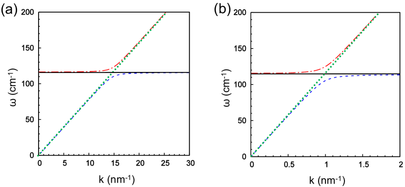
Figure 4: (Color online) Nature and coupling of vibration modes $\omega(k)$ of a carbon nanotube that may be filled with water. (a) Coupling between the dispersionless RBM of a CNT, shown by the black line, and the pressure wave of water enclosed in the CNT, shown by the green dotted line. (b) Coupling between the RBM of a CNT, shown by the black line, and the longitudinal acoustic mode of the CNT, shown by the green dotted line. Results are presented for a CNT with a radius of 1 nm.

Next we consider a long-wavelength displacement wave $u_{x}=u_{x,0}\exp[i(kx-{\omega}t)]$ of small frequency $\omega$ and wave vector $k$ travelling down the liquid column filling a carbon nanotube. We assume the liquid to be compressible but viscosity-free. Thus, the travelling displacement wave will result in a pressure wave $p=p_{0}\exp[i(kx-{\omega}t)]$ that causes radial displacements $r=r_{0}\exp[i(kx-{\omega}t)]$ in the CNT wall. These radial displacements couple the pressure wave in the liquid to the RBM, but not the longitudinal and torsional modes of the CNT.

At small frequencies $\omega$, there will be little radial variation in the pressure. The local compressive strain in the liquid will thus be

$$-\frac{\delta V}{V}=-\left(\frac{\partial u_{x}}{\partial x}+\frac{2r}{R}\right)$$ (A33)

and the pressure becomes

$$p=-B\frac{\delta V}{V}=-B\left(\frac{\partial u_{x}}{\partial x}+\frac{2r}{R}\right)\,.$$ (A34)

Here, $B$ is the bulk modulus of the filling liquid, which we assume is water with $B=2.2{\cdot}10^{9}$ Pa.

The local acceleration of water is given by

$${\rho}_{l}\frac{{\partial}^{2}u_{x}}{{\partial}t^{2}}=-\frac{\partial p}{\partial x}$$ (A35)

and the radial acceleration of the CNT is given by

$${\rho}_{2D}\frac{{\partial}^{2}r}{{\partial}t^{2}}=p-\frac{c_{11}}{R^{2}}r\,.$$ (A36)

Inserting harmonic solutions for $p$, $u_{x}$ and $r$ into Eqs. (A34)-(A36), we obtain

$$\mkern-50.0mu\left(\begin{array}[]{ccc}1&Bik&2B/R\\ -ik&{\rho}_{l}{\omega}^{2}&0\\ 1&0&-(c_{11}/{R^{2}}-{\rho}_{2D}{\omega}^{2})\end{array}\right)\mkern-10.0mu\left(\begin{array}[]{c}p_{0}\\ u_{x,0}\\ r_{0}\end{array}\right)=0$$ (A43)

with the characteristic equation

$$\left(\frac{c_{11}}{R^{2}}-{\rho}_{2D}{\omega}^{2}\right)\left(k^{2}B-{\rho}_{l}{\omega}^{2}\right)-{\rho}_{l}{\omega}^{2}\frac{2B}{R}=0\,.$$ (A44)

This can be rewritten as

$$\left({\omega}_{0}^{2}-{\omega}^{2}\right)\left(k^{2}v^{2}-{\omega}^{2}\right)-{\omega}^{2}{\gamma}^{2}=0\,,$$ (A45)

where ${\omega}_{0}^{2}={c_{11}}/({\rho}_{2D}R^{2})$ and ${\gamma}^{2}={2B}/({\rho}_{2D}R)$. For a CNT of radius $R=1$ nm, we obtain ${\omega}_{0}^{2}=474~{}$ps^-2 and ${\gamma}^{2}=5.92~{}$ps^-2.

Solving Eq. (A45) leads to the dispersion relation $\omega(k)$, which is presented in Fig. 4(a). In the following, we focus on the lowest lying branch of the dispersion relation describing a long wavelength, low frequency pressure wave travelling down the liquid column. In this case, we can neglect $\omega^{2}$ in the first factor of Eq. (A45) and obtain

$$\omega=\frac{vk}{\sqrt{1+\frac{\gamma^{2}}{\omega_{0}^{2}}}}\,.$$ (A46)

Considering the filling liquid to be water with the speed of sound $v=\sqrt{B/{\rho}_{l}}{\approx}1483$ m/s, the velocity of the propagating pressure wave inside the CNT becomes

$$\frac{\omega}{k}=v\frac{1}{\sqrt{1+\frac{\gamma^{2}}{\omega_{0}^{2}}}}=1474~{}{\rm m/s}\,.$$ (A47)

This value is only slightly reduced from that of bulk water because of the relative rigidity of the CNT.

In the corresponding low wavenumber range, the frequency of the RBM is changed to

$$\tilde{\omega}_{RBM}=\omega_{RBM}{\sqrt{1+\frac{\gamma^{2}}{\omega_{RBM}^{2}}}}\,.$$ (A48)

For a CNT with radius $R=1$ nm, $(1+\gamma^{2}/\omega_{RBM}^{2})^{1/2}=(1+5.92/474)^{1/2}=1.006$, yielding only a $0.6$% increase in frequency.

The situation is quite different for tubulin microtubules. Assuming a radius of $R=12.8$ nm, we find $\omega_{RBM}=0.24$ cm^-1 corresponding to $\omega_{RBM}^{2}=0.00203$ ps^-2. In that case, $(1+\gamma^{2}/\omega_{RBM}^{2})^{1/2}=(1+0.0859/0.00203)^{1/2}=6.6$. In other words, filling tubulin microtubules with water will increase their RBM frequency by a factor of 6.6.

As seen in the full solution of Eq. (A45) in Fig. 4(a), at $k{\approx}15$ nm^-1, there is level repulsion and interchange in character between the two dispersion curves. At very much higher frequencies there will be radial modes in the water column that will couple to the RBM of the CNT. These lie outside the scope of the present treatment.

D D. Coupling Between the LA Mode and the RBM in Carbon Nanotubes

Consider a longitudinal wave travelling along a CNT containing no liquid. The CNT of radius $R$ is aligned along the $x-$direction and can be thought of as a rolled up plate in the $xy-$plane with a width of $2{\pi}R$ along the $y-$direction. Where the CNT is being locally stretched, it will narrow down and where it is compressed, it will fatten due to the nonzero value of $c_{12}$ reflected in the Poisson ratio. For longitudinal displacement $u_{x}$ and radial displacement $r$, the strains will be $\epsilon_{11}={\partial u_{x}}/{\partial x}$ and $\epsilon_{22}={r}/{R}$.

The strain energy density is then

$$\begin{split}U&=\frac{1}{2}\left(c_{11}\epsilon_{11}^{2}+c_{11}\epsilon_{22}^{2}+2c_{12}\epsilon_{22}\epsilon_{11}\right)\\ &=\frac{1}{2}c_{11}\left(\left(\frac{\partial u_{x}}{\partial x}\right)^{2}+\left(\frac{r}{R}\right)^{2}\right)+c_{12}\frac{\partial u_{x}}{\partial x}\frac{r}{R}\end{split}$$ (A49)

and the kinetic energy density is

$$T=\frac{1}{2}{\rho}_{2D}\left(\left(\frac{{\partial}u_{x}}{{\partial}t}\right)^{2}+\left(\frac{\partial r}{\partial t}\right)^{2}\right)\,.$$ (A50)

There are two Euler-Langrange equations for the radial and the axial motion,

$$\frac{d}{dt}\left(\frac{\partial\mathcal{L}}{\partial(\frac{dr}{dt})}\right)-\frac{\partial\mathcal{L}}{\partial r}=0$$ (A51)

and

$$\frac{d}{dt}\left(\frac{\partial\mathcal{L}}{\partial(\frac{du_{x}}{dt})}\right)+\frac{\partial}{\partial x}\left(\frac{\partial\mathcal{L}}{\partial(\frac{du_{x}}{dx})}\right)=0\,.$$ (A52)

With the Lagrangian $\mathcal{L}=T-U$ given by Eqs. (A49)-(A50), the Euler-Lagrange equations translate to partial differential equations

$${\rho}_{2D}\frac{\partial^{2}r}{\partial t^{2}}+c_{11}\frac{r}{R^{2}}+\frac{c_{12}}{R}\frac{\partial u_{x}}{\partial x}=0$$ (A53)

and

$${\rho}_{2D}\frac{\partial^{2}u_{x}}{\partial t^{2}}-c_{11}\frac{\partial^{2}u_{x}}{\partial x^{2}}-\frac{c_{12}}{R}\frac{\partial r}{\partial x}=0\,.$$ (A54)

Assuming harmonic solutions $u_{x}=u_{x,0}\exp[i(kx-{\omega}t)]$ and $r=r_{0}\exp[i(kx-{\omega}t)]$, we get

$$\left(\begin{array}[]{cc}-{\rho}_{2D}{\omega}^{2}+c_{11}/R^{2}&ikc_{12}/R\\ -ikc_{12}/R&-{\rho}_{2D}{\omega}^{2}+c_{11}k^{2})\end{array}\right)\left(\begin{array}[]{c}r_{0}\\ u_{x,0}\end{array}\right)=0$$ (A59)

(A60)

with the characteristic equation

$$\left(\frac{c_{11}}{{\rho_{2D}}R^{2}}-{\omega}^{2}\right)\left(\frac{c_{11}}{{\rho_{2D}}}k^{2}-{\omega}^{2}\right)-\frac{c_{12}^{2}k^{2}}{{\rho_{2D}}^{2}R^{2}}=0\,.$$ (A61)

Solving Eq. (A61) leads to the dispersion relations ${\omega}(k)$ that are shown in Fig. 4(b) for a CNT with radius $R=1$ nm, with the values ${c_{11}}/(\rho_{2D}R^{2})=474$ ps^-2, ${c_{11}}/(\rho_{2D})=474$ ps^-2nm² and ${c_{12}^{2}}/(\rho_{2D}^{2}R^{2})=6434$ nm²ps^-4. Our results in Fig. 4(b) closely resemble those of Ref. Wang et al. (2006), obtained using a more complex formalism describing orthotropic elastic cylindrical shells using somewhat different input parameters. Were $c_{12}$ to be zero, then the uncoupled solutions would be the dispersionless RBM of frequency

$$\omega=\frac{1}{R}\sqrt{\frac{c_{11}}{\rho_{2D}}}\,,$$ (A62)

shown by the black solid line in Fig. 4(b), and the pure longitudinal mode of velocity

$$v=\frac{\omega}{k}=\sqrt{\frac{c_{11}}{\rho_{2D}}}\,,$$ (A63)

shown by the green dotted line in Fig. 4(b).

The coupling term induces level repulsion between the ${\omega}_{-}(k)$ and ${\omega}_{+}(k)$ branches, with strong mode hybridization occurring near $k{\approx}1$ nm^-1. It is of interest to examine the limiting forms of the two solutions for $k{\to}0$ and $k{\to}\infty$.

For $k{\to}0$, the larger solution ${\omega}_{+}(k)$ approaches a constant value $\omega_{+}^{0}$. From Eq. (A61) we obtain

$$\omega_{+}^{0}=\frac{1}{R}\sqrt{\frac{c_{11}}{\rho_{2D}}}+\mathcal{O}\left(k^{2}\right)\,.$$ (A64)

The lower solution ${\omega}_{-}(k)$ approaches the value $\omega_{-}=vk$, where $v$ is the velocity of longitudinal mode, modified by its coupling to the RBM. Inserting this in Eq. (A61) and taking the limit $k{\to}0$, we obtain

$$v=\frac{\omega}{k}=\sqrt{\frac{c_{11}\left(1-\alpha^{2}\right)}{\rho_{2D}}}\,,$$ (A65)

where $\alpha=c_{12}/c_{11}$ is the Poisson ratio. The numerical value of the velocity obtained using this expression, $v=21.45$ nm/ps, is slightly smaller than the velocity of the longitudinal mode

$$v=\frac{\omega}{k}=\sqrt{\frac{c_{11}}{\rho_{2D}}}\,,$$ (A66)

which turns out to be $v=21.77$ nm/ps. The 1% reduction by the factor of $\sqrt{1-\alpha^{2}}$ is caused by the coupling of the longitudinal mode to the RBM.

In the opposite limit $k{\to}\infty$, the lower solution ${\omega}_{-}(k)$ approaches a value, which is a little below the uncoupled RBM frequency Liu et al. (2016) of a nanotube with $R=1$ nm,

$$\omega=\frac{1}{R}\sqrt{\frac{c_{11}}{\rho_{2D}}}=117~{}{\rm cm}^{-1}\,.$$ (A67)

We can obtain the coupled RBM frequency $\omega_{-}^{\infty}$ from Eq. (A61) by neglecting its value in comparison with $c_{11}k^{2}/\rho_{2D}$. This yields

$$\omega=\frac{1}{R}\sqrt{\frac{c_{11}\left(1-\alpha^{2}\right)}{\rho_{2D}}}=115~{}{\rm cm}^{-1}\,.$$ (A68)

The 1% reduction of the RMB frequency in the $k{\to}\infty$ limit by the factor of $\sqrt{1-\alpha^{2}}$ is again caused by the coupling of the longitudinal mode to the RBM.

For $k{\to}\infty$, the upper solution approaches the value $\omega_{+}=vk$, where $v$ is the velocity of the uncoupled LA mode. Neglecting ${c_{11}}/(\rho_{2D}R)$ in comparison with $v^{2}k^{2}$ and neglecting $k^{2}$ terms in comparison with $k^{4}$ terms in Eq. (A61), we arrive at

$$v=\sqrt{{c_{11}}/{\rho_{2D}}}$$ (A69)

with no corrections due to the coupling to the RBM. This was to be expected, since for $kR{\gg}1$, this nanotube mode corresponds to the LA mode in a graphene sheet.

References

- Jorio et al. (2008) A. Jorio, M.S. Dresselhaus, and G. Dresselhaus, Carbon Nanotubes: Advanced Topics in the Synthesis, Structure, Properties and Applications, Topics in Applied Physics No. 111 (Springer, Berlin, 2008).
- Overney et al. (1993) G. Overney, W. Zhong, and D. Tomanek, “Structural rigidity and low-frequency vibrational modes of long carbon tubules,” Z. Phys D: Atoms, Molecules and Clusters 27, 93–96 (1993).
- Sazonova et al. (2004) Vera Sazonova, Yuval Yaish, Hande Üstünel, David Roundy, Tomás A. Arias, and Paul L. McEuen, “A tunable carbon nanotube electromechanical oscillator,” Nature 431, 284–287 (2004).
- Wang and Varadan (2006) Q. Wang and V. K. Varadan, “Vibration of carbon nanotubes studied using nonlocal continuum mechanics,” Smart Mater. Struct. 15, 659 (2006).
- Gibson et al. (2007) Ronald F. Gibson, Emmanuel O. Ayorinde, and Yuan-Feng Wen, “Vibrations of carbon nanotubes and their composites: A review,” Comp. Sci. Technol. 67, 1 – 28 (2007).
- Roukes (2001) M. Roukes, “Plenty of room, indeed,” Sci. Am. 285, 48–57 (2001).
- Majee and Aksamija (2016) Arnab K. Majee and Zlatan Aksamija, “Length divergence of the lattice thermal conductivity in suspended graphene nanoribbons,” Phys. Rev. B 93, 235423 (2016).
- Ling et al. (2010) Miao Ling, Liu Hui-Jun, Hu Yi, Zhou Xiang, Hu Cheng-Zheng, and Shi Jing, “Phonon dispersion relations and soft modes of 4 Å carbon nanotubes,” Chinese Phys. B 19, 016301 (2010).
- Love (1927) A. E. H. Love, A treatise on the mathematical theory of elasticity (Cambridge University Press, Cambridge, UK, 1927).
- Liu et al. (2016) Dan Liu, Arthur G. Every, and David Tománek, “Continuum approach for long-wavelength acoustic phonons in quasi-two-dimensional structures,” Phys. Rev. B 94, 165432 (2016).
- Qian et al. (2007) X. S. Qian, J. Q. Zhang, and C. Q. Ru, “Wave propagation in orthotropic microtubules,” J. Appl. Phys. 101, 084702 (2007).
- Sirenko et al. (1996) Yuri M. Sirenko, Michael A. Stroscio, and K. W. Kim, “Elastic vibrations of microtubules in a fluid,” Phys. Rev. E 53, 1003–1010 (1996).
- Wang et al. (2006) C.Y. Wang, C.Q. Ru, and A. Mioduchowski, “Vibration of microtubules as orthotropic elastic shells,” Physica E 35, 48–56 (2006).
- Lawler et al. (2006) H. M. Lawler, J. W. Mintmire, and C. T. White, “Helical strain in carbon nanotubes: Speed of sound and Poisson ratio from first principles,” Phys. Rev. B 74, 125415 (2006).
- Secchi et al. (2016) Eleonora Secchi, Sophie Marbach, Antoine Niguès, Derek Stein, Alessandro Siria, and Lydéric Bocquet, “Massive radius-dependent flow slippage in carbon nanotubes,” Nature 537, 210–213 (2016).
- Artacho et al. (2008) Emilio Artacho, E. Anglada, O. Dieguez, J. D. Gale, A. Garcia, J. Junquera, R. M. Martin, P. Ordejon, J. M. Pruneda, D. Sanchez-Portal, and J. M. Soler, “The SIESTA method; developments and applicability,” J. Phys. Cond. Mat. 20, 064208 (2008).
- Perdew et al. (1996) John P. Perdew, Kieron Burke, and Matthias Ernzerhof, “Generalized gradient approximation made simple,” Phys. Rev. Lett. 77, 3865–3868 (1996).
- Troullier and Martins (1991) N. Troullier and J. L. Martins, “Efficient pseudopotentials for plane-wave calculations,” Phys. Rev. B 43, 1993–2006 (1991).
- Monkhorst and Pack (1976) Hendrik J. Monkhorst and James D. Pack, “Special points for Brillouin-zone integrations,” Phys. Rev. B 13, 5188–5192 (1976).
- Politano et al. (2012) Antonio Politano, Antonio Raimondo Marino, Davide Campi, Daniel Farías, Rodolfo Miranda, and Gennaro Chiarello, “Elastic properties of a macroscopic graphene sample from phonon dispersion measurements,” Carbon 50, 4903–4910 (2012).
- Sánchez-Portal et al. (1999) Daniel Sánchez-Portal, Emilio Artacho, José M. Soler, Angel Rubio, and Pablo Ordejón, “Ab initio structural, elastic, and vibrational properties of carbon nanotubes,” Phys. Rev. B 59, 12678–12688 (1999).
- Maultzsch et al. (2005) J. Maultzsch, H. Telg, S. Reich, and C. Thomsen, “Radial breathing mode of single-walled carbon nanotubes: Optical transition energies and chiral-index assignment,” Phys. Rev. B 72, 205438 (2005).
- Lu et al. (2009) Qiang Lu, Marino Arroyo, and Rui Huang, “Elastic bending modulus of monolayer graphene,” J. Phys. D: Appl. Phys. 42, 102002 (2009).
- Venier et al. (1994) Pascal Venier, Anthony C. Maggs, Marie-France Carlier, and Dominique Pantaloni, “Analysis of microtubule rigidity using hydrodynamic flow and thermal fluctuations.” J. Biol. Chem. 269, 13353–13360 (1994).
- Felgner et al. (1996) H. Felgner, R. Frank, and M. Schliwa, “Flexural rigidity of microtubules measured with the use of optical tweezers,” J. Cell Sci. 109, 509–516 (1996).
- Kikumoto et al. (2006) Mahito Kikumoto, Masashi Kurachi, Valer Tosa, and Hideo Tashiro, “Flexural rigidity of individual microtubules measured by a buckling force with optical traps,” Biophys. J. 90, 1687–1696 (2006).
- Wu et al. (1985) Hsin-I. Wu, Richard D. Spence, Peter J.H. Sharpe, and John D. Goeschl, “Cell wall elasticity: I. A critique of the bulk elastic modulus approach and an analysis using polymer elastic principles,” Plant Cell Environ. 8, 563–570 (1985).
- Chuang et al. (2015) Chern Chuang, Jie Guan, David Witalka, Zhen Zhu, Bih-Yaw Jin, and David Tománek, “Relative stability and local curvature analysis in carbon nanotori,” Phys. Rev. B 91, 165433 (2015).