(Quasi)Periodicity Quantification in Video Data, Using Topology
Abstract
This work introduces a novel framework for quantifying the presence and strength of recurrent dynamics in video data. Specifically, we provide continuous measures of periodicity (perfect repetition) and quasiperiodicity (superposition of periodic modes with non-commensurate periods), in a way which does not require segmentation, training, object tracking or 1-dimensional surrogate signals. Our methodology operates directly on video data. The approach combines ideas from nonlinear time series analysis (delay embeddings) and computational topology (persistent homology), by translating the problem of finding recurrent dynamics in video data, into the problem of determining the circularity or toroidality of an associated geometric space. Through extensive testing, we show the robustness of our scores with respect to several noise models/levels; we show that our periodicity score is superior to other methods when compared to human-generated periodicity rankings; and furthermore, we show that our quasiperiodicity score clearly indicates the presence of biphonation in videos of vibrating vocal folds, which has never before been accomplished end to end quantitatively.
1 Introduction
Periodicity characterizes many natural motions including animal locomotion (walking/wing flapping/slithering), spinning wheels, oscillating pendulums, etc. Quasiperiodicity, thought of as the superposition of non-commensurate frequencies, occurs naturally during transitions from ordinary to chaotic dynamics [11]. The goal of this work is to automate the analysis of videos capturing periodic and quasiperiodic motion. In order to identify both classes of motion in a unified framework, we generalize 1-dimensional (1D) sliding window embeddings [38] to reconstruct periodic and quasiperiodic attractors from videos111Some of the analysis and results appeared as part of the Ph.D. thesis of the first author [tralie2017geometric].222Code to replicate results: https://github.com/ctralie/SlidingWindowVideoTDA333Supplementary material and videos: https://www.ctralie.com/Research/SlidingWindowVideoQuasi. We analyze the resulting attractors using persistent homology, a technique which combines geometry and topology (Section 2.2), and we return scores in the range that indicate the degree of periodicity or quasiperiodicity in the corresponding video. We show that our periodicity measure compares favorable to others in the literature when ranking videos (Section 4.2). Furthermore, to our knowledge, there is no other method able to quantify the existence of quasiperiodicity directly from video data.
Our approach is fundamentally different from most others which quantify periodicity in video. For instance, it is common to derive 1D signals from the video and apply Fourier or autocorrelation to measure periodicity. By contrast, our technique operates on raw pixels, avoiding common video preprocessing and tracking entirely. Using geometry over Fourier/autocorrelation also has advantages for our applications. In fact, as a simple synthetic example shows (Figure 3), the Fourier Transform of quasiperiodic signals is often very close to the Fourier transform of periodic signals. By contrast, the sliding window embeddings we design yield starkly different geometric structures in the periodic and quasiperiodic cases. We exploit this to devise a quasiperiodicity measurement, which we use to indicate the degree of “biphonation” in videos of vibrating vocal folds (Section 4.3), which is useful in automatically diagnosing speech pathologies.
In the context of applied topology, our quasiperiodicity score is one of the first applications of persistent to high dimensional data, which is largely possible due to recent advancements in the computational feasibility of persistent homology [3].
1.1 Prior Work on Recurrence in Videos
1.1.1 1D Surrogate Signals
One common strategy for detecting periodicity in video is to derive a 1D function to act as a surrogate for its dynamics, and then to use either frequency domain (Fourier transform) or time domain (autocorrelation, peak finding) techniques. One of the earliest works in this genre finds level set surfaces in a spatiotemporal “XYT” volume of video (all frames stacked on top of each other), and then uses curvature scale space on curves that live on these “spatiotemporal surfaces” as the 1D function [1]. [34] use Fourier Transforms on pixels which exhibit motion, and define a measure of periodicity based on the energy around the Fourier peak and its harmonics. [10] extract contours and find eigenshapes from the contours to classify and parameterize motion within a period. Frequency estimation is done by using Fourier analysis and peak detection on top of other 1D statistics derived from the contours, such as area and center of mass. Finally, [47] derive a 1D surrogate function based on mutual information between the first and subsequent frames, and then look for peaks in the similarity function with the help of a watershed method.
1.1.2 Self-Similarity Matrices
Another class of techniques relies on self-similarity matrices (SSMs) between frames, where similarity can be defined in a variety of ways. [37] track a set of points on a foreground object and compare them with an affine invariant similarity. Another widely recognized technique for periodicity quantification [6], derives periodicity measures based on self-similarity matrices of L1 pixel differences. This technique has inspired a diverse array of applications, including analyzing the cycles of expanding/contracting jellyfish [33], analyzing bat wings [2], and analyzing videos of autistic spectrum children performing characteristic repetitive motions such as “hand flapping” [22]. We compare to this technique in Section 4.2.
1.1.3 Miscellaneous Techniques for Periodic Video Quantification
There are also a number of works that don’t fall into the two categories above. Some works focus solely on walking humans, since that is one of the most common types of periodic motion in videos of interest to people. [29] look at the “braiding patterns” that occur in XYT slices of videos of walking people. [17] perform blob tracking on the foreground of a walking person, and use the ratio of the second and first eigenvalues of PCA on that blob.
For more general periodic videos, [43] make a codebook of visual words and look for repetitions within the resulting string. [23] take a deep learning approach to counting the number of periods that occur in a video segment. They use a 3D convolutional neural network on spatially downsampled, non-sequential regions of interest, which are uniformly spaced in time, to estimate the length of the cycle. Finally, perhaps the most philosophically similar work to ours is the work of [41], who use cohomology to find maps of MOCAP data to the circle for parameterizing periodic motions, though this work does not provide a way to quantify periodicity.
1.1.4 Our Work
We show that geometry provides a natural way to quantify recurrence (i.e. periodicity and quasiperiodicity) in video, by measuring the shape of delay embeddings. In particular, we propose several optimizations (section 3) which make this approach feasible. The resulting measure of quasiperiodicity, for which quantitative approaches are lacking, is used in section 4.3 to detect anomalies in high-speed videos of vibrating vocal folds. Finally, in contrast to both frequency and time domain techniques, our method does not rely on the period length being an integer multiple of the sampling rate.
2 Background
2.1 Delay Embeddings And Their Geometry
Recurrence in video data can be captured via the geometry of delay embeddings; we describe this next.
2.1.1 Video Delay Embeddings
We will regard a video as a sequence of grayscale444For color videos we can treat each channel independently, yielding a vector in . In practice, there isn’t much of a difference between color and grayscale embeddings in our framework for the videos we consider. image frames indexed by the positive real numbers. That is, given positive integers (width) and (height), a video with pixels is a function
In particular, a sequence of images sampled at discrete times yields one such function via interpolation. For an integer , known as the dimension, a real number , known as the delay, and a video , we define the sliding window (also referred to as time delay) embedding of – with parameters and – at time as the vector
| (1) |
The subset of resulting from varying will be referred to as the sliding window embedding of . We remark that since the pixel measurement locations are fixed, the sliding window embedding is an “Eulerian” view into the dynamics of the video. Note that delay embeddings are generally applied to 1D time series, which can be viewed as 1-pixel videos () in our framework. Hence equation (1) is essentially the concatenation of the delay embeddings of each individual pixel in the video into one large vector. One of the main points we leverage in this paper is the fact that the geometry of the sliding window embedding carries fundamental information about the original video. We explore this next.
2.1.2 Geometry of 1-Pixel Video Delay Embeddings
As a motivating example, consider the harmonic (i.e. periodic) signal
| (2) |
and the quasiperiodic signal
| (3) |
We refer to as harmonic because its constitutive frequencies, and , are commensurate; that is, they are linearly dependent over the rational numbers . By way of contrast, the underlying frequencies of the signal , and , are linearly independent over and hence non-commensurate. We use the term quasiperiodicity, as in the non-linear dynamics literature [19], to denote the superposition of periodic processes whose frequencies are non-commensurate. This differs from other definitions in the literature (e.g. [43, robinson2016topological]) which regard quasiperiodic as any deviation from perfect repetition.
A geometric argument from [31] (see equation 7 below and the discussion that follows) shows that given a periodic function with exactly harmonics, if and then the sliding window embedding is a topological circle (i.e. a closed curve without self-intersections) which wraps around an -dimensional torus
As an illustration, we show in Figure 1 a plot of and of its sliding window embedding , via a PCA (Principal Component Analysis) 3-dimensional projection.
However, if is quasiperiodic with distinct non-commensurate frequencies then, for appropriate and , is dense in (i.e. fills out) [30]. Figure 2 shows a plot of the quasiperiodic signal and a 3-dimensional projection, via PCA, of its sliding window embedding .
The difference in geometry of the delay embeddings is stark compared to the difference between their power spectral densities, as shown in Figure 3.
Moreover, as we will see next, the interpretation of periodicity and quasiperiodicity as circularity and toroidality of sliding window embeddings remains true for videos with higher resolution (i.e. ). The rest of the paper will show how one can use persistent homology, a tool from the field of computational topology, to quantify the presence of (quasi)periodicity in a video by measuring the geometry of its associated sliding window embedding. In short, we propose a periodicity score for a video which measures the degree to which the sliding window embedding spans a topological circle, and a quasiperiodicity score which quantifies the degree to which covers a torus. This approach will be validated extensively: we show that our (quasi)periodicity detection method is robust under several noise models (motion blur, additive Gaussian white noise, and MPEG bit corruption); we compare several periodicity quantification algorithms and show that our approach is the most closely aligned with human subjects; finally, we provide an application to the automatic classification of dynamic regimes in high-speed laryngeal video-endoscopy.
2.1.3 Geometry of Video Delay Embeddings
Though it may seem daunting compared to the 1D case, the geometry of the delay embedding shares many similarities for periodic videos, as shown in [39]. Let us argue why sliding window embeddings from (quasi)periodic videos have the geometry we have described so far. To this end, consider an example video that contains a set of frequencies . Let the amplitude of the frequency and pixel be . For simplicity, but without loss of generality, assume that each is a cosine with zero phase offset. Then the time series at pixel can be written as
| (4) |
Grouping all of the coefficients together into a matrix , we can write
| (5) |
where stands for the column of . Constructing a delay embedding as in Equation 1:
| (6) |
and applying the cosine sum identity, we get
| (7) |
where are constant vectors. In other words, the sliding window embedding of this video is the sum of linearly independent ellipses, which lie in the space of frame videos at resolution . As shown in [31] for the case of commensurate frequencies, when the window length is just under the length of the period, all of the and vectors become orthogonal, and so they can be recovered by doing PCA on . Figure 4 shows the components of the first 8 PCA vectors for a horizontal line of pixels in a video of an oscillating pendulum. Note how the oscillations are present both temporally and spatially.
2.1.4 The High Dimensional Geometry of Repeated Pulses
Using Eulerian coordinates has an important impact on the geometry of delay embeddings of natural videos. As Figure 5 shows, pixels often jump from foreground to background in a pattern similar to square waves.
These types of abrupt transitions require higher dimensional embeddings to reconstruct the geometry. To see why, first extract one period of a signal with period at a pixel :
| (8) |
Then can be rewritten in terms of the pulse as
| (9) |
Since repeats itself, regardless of what looks like, periodic summation discretizes the frequency domain [32]
| (10) |
Switching back to the time domain, we can write as
| (11) |
In other words, each pixel is the sum of some constant offset plus a (possibly infinite) set of harmonics at integer multiples of . For instance, applying Equation 11 to a square wave of period centered at the origin is a roundabout way of deriving the Fourier Series
| (12) |
by sampling the sinc function at intervals of (every odd coincides with , proportional to , and every even harmonic is zero conciding with ). In general, the sharper the transitions are in , the longer the tail of will be, and the more high frequency harmonics will exist in the embedding, calling for a higher delay dimension to fully capture the geometry, since every harmonic lives on a linearly independent ellipse. Similar observations about harmonics have been made in images for collections of patches around sharp edges ([48], Figure 2).
2.2 Persistent Homology
Informally, topology is the study of properties of spaces which do not change after stretching without gluing or tearing. For instance, the number of connected components and the number of (essentially different) 1-dimensional loops which do not bound a 2-dimensional disk, are both topological properties of a space. It follows that a circle and a square are topologically equivalent since one can deform one onto the other, but a circle and a line segment are not because that would require either gluing the endpoints of the line segment or tearing the circle. Homology [12] is a tool from algebraic topology designed to measure these types of properties, and persistent homology [50] is an adaptation of these ideas to discrete collections of points (e.g., sliding window embeddings). We briefly introduce these concepts next.
2.2.1 Simplicial Complexes
A simplicial complex is a combinatorial object used to represent and discretize a continuous space. With a discretization available, one can then compute topological properties by algorithmic means. Formally, a simplicial complex with vertices in a nonempty set is a collection of nonempty finite subsets so that always implies . An element is called a simplex, and if has elements then it is called an -simplex. The cases are special, 0-simplices are called vertices, 1-simplices are called edges and 2-simplices are called faces. Here is an example to keep in mind: the circle is a continuous space but its topology can be captured by a simplicial complex with three vertices , and three edges , , . That is, in terms of topological properties, the simplicial complex
can be regarded as a combinatorial surrogate for : they both have 1 connected component, one 1-dimensional loop which does not bound a 2-dimensional region, and no other features in higher dimensions.
2.2.2 Persistent Homology of Point Clouds
The sliding window embedding of a video is, in practice, a finite set determined by a choice of finite. Moreover, since then the restriction of the ambient Euclidean distance endows with the structure of a finite metric space. Discrete metric spaces, also referred to as point clouds, are trivial from a topological point of view: a point cloud with points simply has connected components and no other features (e.g., holes) in higher dimensions. However, when a point cloud has been sampled from/around a continuous space with non-trivial topology (e.g., a circle or a torus), one would expect that appropriate simplicial complexes with vertices on the point cloud should reflect the topology of the underlying continuous space. This is what we will exploit next.
Given a point cloud – where is a finite set and is a distance function – the Vietoris-Rips complex (or Rips complex for short) at scale is the collection of non-empty subsets of with diameter less than or equal to :
| (13) |
That is, is the simplicial complex with vertex set equal to , constructed by adding an edge between any two vertices which are at most apart, adding all 2-dimensional triangular faces (i.e. 2-simplices) whose bounding edges are present, and more generally, adding all the -simplices whose -dimensional bounding facets have been included. We show in Figure 6 the evolution of the Rips complex on a set of points sampled around the unit circle.
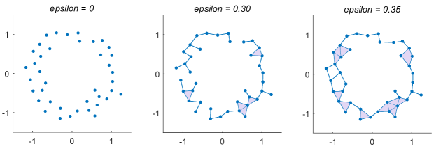
The idea behind persistent homology is to track the evolution of topological features of complexes such as , as the scale parameter ranges from to some maximum value . For instance, in Figure 6 one can see that has 40 distinct connect components (one for each point), has three connected components and has only one connected component; this will continue to be the case for every . Similarly, there are no closed loops in or bounding empty regions, but this changes when increases to . Indeed, has three 1-dimensional holes: the central prominent hole, and the two small ones to the left side. Notice, however, that as increases beyond these holes will be filled by the addition of new simplices; in particular, for one has that will have only one connected component and no other topological features in higher dimensions.
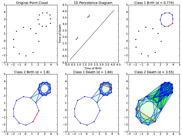
The family is known as the Rips filtration of , and the emergence/dissapearence of topological features in each dimension (i.e., connected components, holes, voids, etc) as changes, can be codified in what are referred to as the persistence diagrams of . Specifically, for each dimension (0 = connected components, 1 = holes, 2 = voids, etc) one can record the value of for which a particular -dimensional topological feature of the Rips filtration appears (i.e. its birth time), and when it disappears (i.e. its death time). The birth-death times of -dimensional features for form a multiset — i.e. a set whose elements can come with repetition — known as the -dimensional persistence diagram of the Rips filtration on . Since is just a collection of points in the region , we will visualize it as a scatter plot. The persistence of a topological feature with birth-death times is the quantity , i.e. its lifetime. We will also include the diagonal in the scatter plot in order to visually convey the persistence of each birth-death pair. In this setting, points far from the diagonal (i.e. with large persistence) represent topological features which are stable across scales and hence deemed significant, while points near the diagonal (i.e. with small persistence) are often associated with unstable features. We illustrate in Figure 7 the process of going from a point cloud to the 1-dimensional persistence diagram of its Rips filtration.
We remark that the computational task of determining all non-equivalent persistent homology classes of a filtered simplicial complex can, surprisingly, be reduced to computing the homology of a single simplicial complex [50, 3]. This is in fact a problem in linear algebra that can be solved via elementary row and column operations on appropriate boundary matrices.
The persistent homology of , and in particular its -dimensional persistence diagrams for , are the objects we will use to quantify periodicity and quasiperiodicity in a video . Figures 8 and 9 show the persistence diagrams of the Rips filtrations, on the sliding window embeddings, for the commensurate and non-commensurate signals from Figures 1 and 2, respectively. We use fast new code from the “Ripser” software package to make persistent computation feasible [3].
3 Implementation Details
3.1 Reducing Memory Requirements with SVD
Suppose we have a video which has been discretely sampled at different frames at a resolution of , and we do a delay embedding with dimension , for some arbitrary . Assuming 32 bit floats per grayscale value, storing the sliding window embedding requires bytes. For a low resolution video only 10 seconds long at 30fps, using already exceeds 1GB of memory. In what follows we will address the memory requirements and ensuing computational burden to construct and access the sliding window embedding. Indeed, constructing the Rips filtration only requires pairwise distances between different delay vectors, this enables a few optimizations.
First of all, for points in , where , there exists an -dimensional linear subspace which contains them. In particular let be the matrix with each video frame along a column. Performing a singular value decomposition , yields a matrix whose columns form an orthonormal basis for the aforementioned -dimensional linear subspace. Hence, by finding the coordinates of the original frame vectors with respect to this orthogonal basis
| (14) |
and using the coordinates of the columns of instead of the original pixels, we get a sliding window embedding of lower dimension
| (15) |
for which
Note that can be computed by finding the eigenvectors of ; this has a cost of which is dominated by if . In our example above, this alone reduces the memory requirements from 1GB to 10MB. Of course, this procedure is the most effective for short videos where there are actually many fewer frames than pixels, but this encompasses most of the examples in this work. In fact, the break-even point for a 200x200 30fps video is 22 minutes. A similar approach was used in the classical work on Eigenfaces [40] when computing the principal components over a set of face images.
3.2 Distance Computation via Diagonal Convolutions
A different optimization is possible if ; that is, if delays are taken exactly on frames and no interpolation is needed. In this case, the squared Euclidean distance between and is
| (16) |
Let be the matrix of all pairwise squared Euclidean distances between frames (possibly computed with the memory optimization in Section 3.1), and let be the matrix of all pairwise distances between delay frames. Then Equation 16 implies that can be obtained from via convolution with a “rect function”, or a vector of s of length , over all diagonals in (i.e. a moving average). This can be implemented in time with cumulative sums. Hence, regardless of how is chosen, the computation and memory requirements for computing depend only on the number of frames in the video. Also, can simply be computed by taking the entry wise square root of , another computation. A similar scheme was used in [16] when comparing distances of 3D shape descriptors in videos of 3D meshes.
Figure 10 shows self-similarity matrices on embeddings of the pendulum video with no delay and with a delay approximately matching the period. The effect of a moving average along diagonals with delay eliminates the anti-diagonals caused by the video’s mirror symmetry.
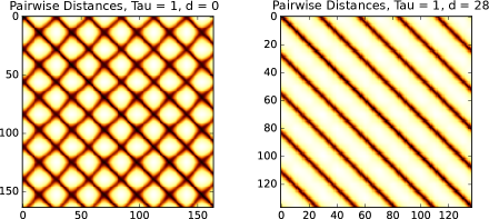
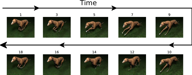
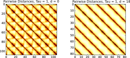
Even for videos without mirror symmetries, such as a video of a running dog (Figure 11), introducing a delay brings the geometry into focus, as shown in Figure 12.
3.3 Normalization
A few normalization steps are needed in order to enable fair comparisons between videos with different resolutions, or which have a different range in periodic motion either spatially or in intensity. First, we perform a “point-center and sphere normalize” vector normalization which was shown in [31] to have nice theoretical properties.
That is,
| (17) |
where is a vector of all ones. In other words, one subtracts the mean of each component of each vector, and each vector is scaled so that it has unit norm (i.e. lives on the unit sphere in ). Subtracting the mean from each component will eliminate additive linear drift on top of the periodic motion, while scaling addresses resolution / magnitude differences. Note that we can still use the memory optimization in Section 3.1, but we can no longer use the optimizations in Section 3.2 since each window is normalized independently.
Moreover, in order to mitigate nonlinear drift, we implement a simple pixel-wise convolution by the derivative of a Gaussian for each pixel in the original video before applying the delay embedding:
| (18) |
This is a pixel-wise bandpass filter which could be replaced with any other bandpass filter leveraging application specific knowledge of expected frequency bounds. This has the added advantage of reducing the number of harmonics, enabling a smaller embedding dimesion .
3.4 Periodicity/Quasiperiodicity Scoring
Once the videos are normalized to the same scale, we can score periodicity and quasiperiodicity based on the geometry of sliding window embeddings. Let be the -dimensional persistence diagram for the Rips filtration on the sliding window embedding of a video, and define as the -th largest difference for . In particular
and . We propose the following scores:
-
1.
Periodicity Score (PS)
(19) Like [31], we exploit the fact that for the Rips filtration on , the 1-dimensional persistence diagram has only one prominent birth-death pair with coordinates . Since this is the limit shape of a normalized perfectly periodic sliding window video, the periodicity score is between 0 (not periodic) and 1 (perfectly periodic).
-
2.
Quasiperiodicity Score (QPS)
(20) This score is designed with the torus in mind. We score based on the second largest 1D persistence times the largest 2D persistence, since we want a shape that has two core circles and encloses a void to get a large score. Based on the Knneth theorem of homology, the 2-cycle (void) should die the moment the smallest 1-cycle dies.
-
3.
Modified Periodicity Score (MPS)
(21) We design a modified periodicity score which should be lower for quasiperiodic videos, than what the original periodicity score would yield.
Note that we use field coefficients for all persistent homology computations since, as shown by [31], this works better for periodic signals with strong harmonics. Before we embark on experiments, let us explore the choice of two crucial parameters for the sliding window embedding: the delay and the dimension . In practice we determine an equivalent pair of parameters: the dimension and the window size .
3.5 Dimension and Window Size
Takens’ embedding theorem is one of the most fundamental results in the theory of dynamical systems [38]. In short, it contends that (under appropriate hypotheses) there exists an integer , so that for all and generic the sliding window embedding reconstructs the state space of the underlying dynamics witnessed by the signal . One common strategy for determining a minimal such is the false nearest-neighbors scheme [21]. The idea is to keep track of the -th nearest neighbors of each point in the delay embedding, and if they change as is increased, then the prior estimates for were too low. This algorithm was used in recent work on video dynamics [42], for instance.
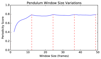
Even if we can estimate , however, how does one choose the delay ? As shown in [31], the sliding window embedding of a periodic signals is roundest (i.e. so that the periodicity score is maximized) when the window size, , satisfies the following relation:
| (22) |
Here is number of periods that the signal has in and . To verify this experimentally, we show in Figure 13 how the periodicity score changes as a function of window size for the pendulum video, and how the choice of window size from Equation 22 maximizes . To generate this figure we fixed a sufficiently large and varied . Let us now describe the general approach: Given a video we perform a period-length estimation step (see section 3.6 next), which results in a positive real number . For a given large enough we let be so that .
3.6 Fundamental Frequency Estimation
Though Figure 13 suggests robustness to window size as long as the window is more than half of the period, we may not know what that is in practice. To automate window size choices, we do a coarse estimate using fundamental frequency estimation techniques on a 1D surrogate signal. To get a 1D signal, we extract the first coordinate of diffusion maps [4] using nearest neighbors on the raw video frames (no delay) after taking a smoothed time derivative. Note that a similar diffusion-based method was also used in recent work by [46] to analyze the frequency spectrum of a video of an oscillating 2 pendulum + spring system in a quasiperiodic state. Once we have the diffusion time series, we then apply the normalized autocorrelation method of [25] to estimate the fundamental frequency. In particular, given a discrete signal of length , define the autocorrelation as
| (23) |
However, as observed by [7], a more robust function for detecting periodicities is the squared difference function
| (24) |
which can be rewritten as where
| (25) |
Finally, [25] suggest normalizing this function to the range to control for window size and to have an interpretation akin to a Pearson correlation coefficient:
| (26) |
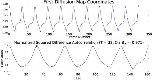
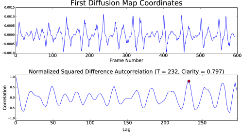
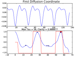
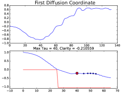
The fundamental frequency is then the inverse period of the largest peak in which is to the right of a zero crossing. The zero crossing condition helps prevent an offset of from being the largest peak. Defining the normalized autocorrelation as in Equation 26 has the added advantage that the value of at the peak can be used to score periodicity, which the authors call clarity. Values closer to 1 indicate more perfect periodicities. This technique will sometimes pick integer multiples of the period, so we multiply by a slowly decaying envelope which is 1 for 0 lag and 0.9 for the maximum lag to emphasize smaller periods. Figure 14 shows the result of this algorithm on a periodic video, and Figure 15 shows the algorithm on an irregular video.
4 Experimental Evaluation
Next we evaluate the effectiveness of the proposed (Modified) Periodicity and Quasiperiodicity scores on three different tasks. First, we provide estimates of accuracy for the binary classifications periodic/not-periodic or quasiperiodic/not-quasiperiodic in the presence of several noise models and noise levels. The results illustrate the robustness of our method. Second, we quantify the quality of periodicity rankings from machine scores, as compared to those generated by human subjects. In a nutshell, and after comparing with several periodicity quantification algorithms, our approach is shown to be the most closely aligned with the perception of human subjects. Third, we demonstrate that our methodology can be used to automatically detect the physiological manifestations of certain speech pathologies (e.g., normal vs. biphonation), directly from high-speed videos of vibrating vocal folds.
4.1 Classification Under Varying Noise Levels/Models
As shown empirically in [8], a common source of noise in videos comes from camera shake (blur); this is captured by point spread functions resembling directed random walks [8, Figure 1] and the amount of blur (i.e. noise level) is controlled by the extent in pixels of the walk. Other sources are additive white Gaussian noise (awgn), controlled by the standard deviation of the Gaussian kernel, and MPEG bit errors quantified by the percentage of corrupted information. Figure 16 shows examples of these noise types.


For classification purposes we use three main recurrence classes. Three types of periodic videos (True periodic, TP): an oscillating pendulum, a bird flapping its wings, and an animation of a beating heart. Two types of quasiperiodic videos (True quasiperiodic, TQ): one showing two solid disks which oscillate sideways at non-commensurate rates, and the second showing two stationary Gaussian pulses with amplitudes non-commensurately modulated by cosine functions. Two videos without significant recurrence (True non-recurrent, TN): a video of a car driving past a landscape, and a video of an explosion. Each one of these seven videos is then corrupted by the three noise models at three different noise levels (blur = 20, 40, 80, awgn 1, 2, 3, bit error = 5, 10, 20%) as follows: given a particular video, a noise model and noise level, 600 instances are generated by sampling noise independently at random.
Results: We report in Table 1 the area under the Receiver Operating Characteristic (ROC) curve, or AUROC for short, for the classification task TP vs. TN (resp. TQ vs. TN) and binary classifier furnished by Periodicity (resp. Quasiperiodicity) Score.
| Blur 20 | Blur 40 | Blur 80 | Awgn | Awgn | Awgn | Bit Err 5% | Bit Err 10% | Bit Err 15% | ||||||||||
| Bird Flapping | 1 | 1 | 1 | 1 | 1 | 1 | 1 | 1 | 1 | 1 | 1 | 1 | 1 | 0.97 | 1 | 0.92 | 0.75 | 0.79 |
| Heart Beat | 1 | 1 | 1 | 1 | 0.91 | 0.94 | 1 | 1 | 1 | 1 | 0.9 | 0.89 | 1 | 0.91 | 0.98 | 0.87 | 0.56 | 0.62 |
| Pendulum | 1 | 0.94 | 0.84 | 0.85 | 0.43 | 0.68 | 1 | 1 | 1 | 1 | 1 | 1 | 1 | 1 | 1 | 0.99 | 0.98 | 0.97 |
| QuasiPeriodic Disks | 1 | 0.85 | 1 | 0.83 | 0.75 | 0.39 | 1 | 1 | 1 | 1 | 1 | 1 | 1 | 0.92 | 0.99 | 0.93 | 0.82 | 0.82 |
| QuasiPeriodic Pulses | 1 | 0.9 | 1 | 0.87 | 1 | 0.83 | 1 | 1 | 1 | 1 | 1 | 1 | 1 | 0.96 | 0.99 | 0.95 | 0.95 | 0.95 |
For instance, for the Blur noise model with noise level of pixels, the AUROC from using the Periodicity Score to classify the 600 instances of the Heartbeat video as periodic, and the 600 instances of the Driving video as not periodic is 0.91. Similarly, for the MPEG bit corruption model with 5% of bit error, the AUROC from using the Quasiperiodicity score to classify the 600 instances of the Quasiperiodic Sideways Disks as quasiperiodic and the 600 instances of the Explosions video as not quasiperiodic is 0.92. To put these numbers in perspective, AUROC = 1 is associated with a perfect classifier and AUROC = 0.5 corresponds to classification by a random coin flip.
Overall, the type of noise that degrades performance the most across videos is the bit error, which makes sense, since this has the effect of randomly freezing, corrupting, or even deleting frames, which all interrupt periodicity. The blur noise also affects videos where the range of motion is small. The pendulum video, for instance, only moves over a range of 60 pixels at the most extreme end, so an 80x80 pixel blur almost completely obscures the motion.
4.2 Comparing Human and Machine Periodicity Rankings
Next we quantify the extent to which rankings obtained from our periodicity score (Equation 19), as well as three other methods, agree with how humans rank videos by periodicity. The starting point is a dataset of 20 different creative commons videos, each 5 seconds long at 30 frames per second. Some videos appear periodic, such as a person waving hands, a beating heart, and spinning carnival rides. Some of them appear nonperiodic, such as explosions, a traffic cam, and drone view of a boat sailing. And some of them are in between, such as the pendulum video with simulated camera shake.
It is known that humans are notoriously bad at generating globally consistent rankings of sets with more than 5 or 7 elements [27]. However, when it comes to binary comparisons of the type “should A be ranked higher than B?” few systems are as effective as human perception, specially for the identification of recurrent patterns in visual stimuli. We will leverage this to generate a globally consistent ranking of the 20 videos in our initial data set.
We use Amazon’s Mechanical Turk (AMT) [5] to present each pair of videos in the set of 20, , each to three different users, for a total of 570 pairwise rankings. 15 unique AMT workers contributed to our experiment, using an interface as the one shown in Figure 17.

In order to aggregate this information into a global ranking which is as consistent as possible with the pairwise comparisons, we implement a technique known as Hodge rank aggregation [18]. Hodge rank aggregation finds the closest consistent ranking to a set of preferences, in a least squares sense. More precisely, given a set of objects , and given a set of comparisons , we seek a scalar function on all of the objects that minimizes the following sum
| (27) |
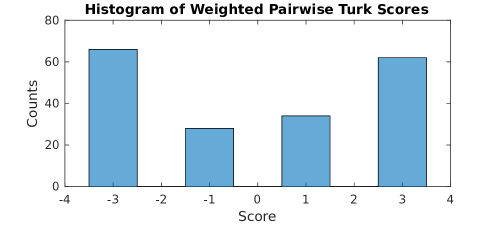
where is a real number which is positive if is ranked higher than and negative otherwise. Thus, is a function whose discrete gradient best matches the set of preferences with respect to an norm. Note that the preferences that we feed the algorithm are based on the pairwise rankings returned from AMT. If video is greater than video , then we assign , or -1 otherwise. Since we have 3 rankings for each video, we actually assign weights of +3, +1, -1, or -3. The +/- 3 are if all rankings agree in one direction, and the +/- 1 are if one of the rankings disagrees with the other two. Figure 18 shows a histogram of all of the weighted scores from users on AMT. They are mostly in agreement, though there are a few +/- 1 scores.
As comparison to the human scores, we use three different classes of techniques for machine ranking of periodicity.
Sliding Windows (SW): We sort the videos in decreasing order of Periodicity Score (Equation 19). We fix the window size at 20 frames and the embedding dimension at 20 frames (which is enough to capture 10 strong harmonics). We also apply a time derivative of width 10 to every frame.
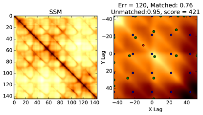
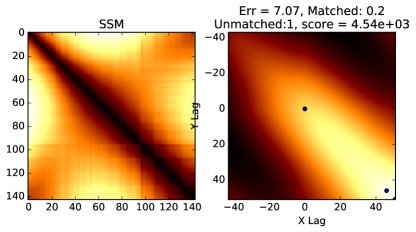
Cutler-Davis [6]: The authors of this work present two different techniques to quantify periodicity from a self-similarity matrix (SSM) of video frames. The first is a frequency domain technique based on the peak of the average power spectral density over all columns (rows) of the SSM after linearly de-trending and applying a Hann window. To turn this into a continuous score, we report the ratio of the peak minus the mean over the standard deviation. This method will be referred to as Frequency Score.
As the authors warn, the frequency peak method has a high susceptibility to false positives. This motivated the design of a more robust technique in [6], which works by finding peaks in the 2D normalized autocorrelation of the Gaussian smoothed SSMs. For videos with mirror symmetry, the peaks will lie on a diamond lattice, while for videos without mirror symmetry, they will lie on a square lattice. After peak finding within neighborhoods, one simply searches over all possible lattices at all possible widths to find the best match with the peaks. Since each lattice is centered at the autocorrelation point , no translational checks are necessary.
To turn this into a continuous score, let be the sum of Euclidean distances of the matched peaks in the autocorrelation image to the best fit lattice, let be the proportion of lattice points that have been matched, and let be the proportion of peaks which have been matched to a lattice point. Then we give the final periodicity score as
| (28) |
A lattice which fits the peaks perfectly () with no error () and no false positive peaks () will have a score of 1, and any video which fails to have a perfectly matched lattice will have a score greater than 1. Hence, we sort in increasing order of the score to get a ranking.
As we will show, this technique agrees the second best with humans after our Periodicity Score ranking. One of the main drawbacks is numerical stability of finding maxes in non-isolated critical points around nearly diagonal regions in square lattices, which will erroneously inflate the score. Also, the lattice searching only occurs over an integer grid, but there may be periods that aren’t integer number of frames, so there will always be a nonzero for such videos. By contrast, our sliding window scheme can work for any real valued period length.
Diffusion Maps + Normalized Autocorrelation “Clarity”: Finally, we apply the technique from Section 3.6 to get an autocorrelation function, and we report the value of the maximum peak of the normalized autocorrelation to the right of a zero crossing, referred to as “clarity” by [25]. Values closer to 1 indicate more perfect repetitions, so we sort in descending order of clarity to get a ranking.
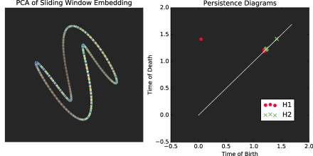
Figure 19 shows an example of these three different techniques on a periodic video. There is a dot which rises above the diagonal in the persistence diagram, a lattice is found which nearly matches the critical points in the autocorrelation image, and autocorrelation function on diffusion maps has a nice peak.
By contrast, for a nonperiodic video (Figure 20), there is hardly any persistent homology, there is no well matching lattice, and the first diffusion coordinate has no apparent periodicities.
Results: Once we have the global human rankings and the global machine rankings, we can compare them using the Kendall score [20]. Given a set of objects objects and two total orders and , where if and if , the Kendall score is defined as
| (29) |
For two rankings which agree exactly, the Kendall score will be 1. For two rankings which are exactly the reverse of each other, the Kendall score will be -1. In this way, it analogous to a Pearson correlation between rankings.
| Human | SW+TDA | Freq[6] | CDscore[6] | Clarity[7] | |
|---|---|---|---|---|---|
| Human | 1 | 0.663 | -0.295 | 0.347 | 0.284 |
| SW+TDA | 0.663 | 1 | -0.316 | 0.221 | 0.516 |
| Freq[6] | -0.295 | -0.316 | 1 | -0.0842 | -0.189 |
| CDscore[6] | 0.347 | 0.221 | -0.0842 | 1 | 0.411 |
| Clarity[7] | 0.284 | 0.516 | -0.189 | 0.411 | 1 |
| SW+TDA | Freq[6] | CDscore[6] | Clarity[7] |
|---|---|---|---|
| 3101ms | 73ms | 176ms | 154ms |
Table 2 shows the Kendall scores between all of the different machine rankings and the human rankings. Our sliding window video methodology (SW+TDA) agrees with the human ranking more than any other pair of ranking types. The second most similar are the SW and the diffusion clarity, which is noteworthy as they are both geometric techniques. Table 3 also shows the average run times, in milliseconds, of the different algorithms on each video on our machine. This does highlight one potential drawback of our technique, since TDA algorithms tend to be computationally intensive. However, at this scale (videos with at most several hundred frames), performance is reasonable.
4.3 Periodicity And Biphonation in High Speed Videos of Vocal Folds
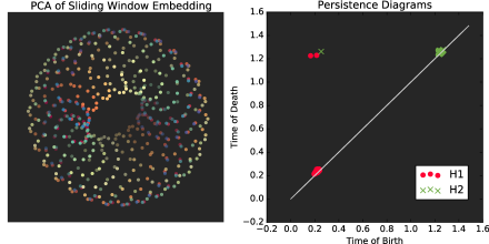
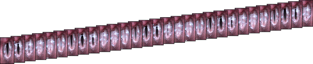
In this final task we apply our methodology to a real world problem of interest in medicine. We show that our method can automatically detect certain types of voice pathologies from high-speed glottography, or high speed videos (4000 fps) of the left and right vocal folds in the human vocal tract [45, 44, 9]. In particular, we detect and differentiate quasiperiodicity from periodicity by using our geometric sliding window pipeline. Quasiperiodicity is a special case of what is referred to as “biphonation” in the biological context, where nonlinear phenomena cause a physical process to bifurcate into two different periodic modes, often during a transition to chaotic behavior [15]. The torus structure we sketched in Figure 9 has long been recognized in this context [28], but we provide a novel way of quantifying it.
Similar phenomena exist in audio [14, 15], but the main reason for studying laryngeal high speed video is understanding the biomechanical underpinnings of what is perceived in the voice. In particular, this understanding can potentially lead to practical corrective therapies and surgical interventions. On the other hand, the presence of biphonation in sound is not necessarily the result of a physiological phenomenon; it has been argued that it may come about as the result of changes in states of arousal [briefer2015segregation].
In contrast with our work, the existing literature on video-based techniques usually employs an inherently Lagrangian approach, where different points on the left and right vocal folds are tracked, and coordinates of these points are analyzed as 1D time series (e.g. [28, 35, 24, 13], [26]). This is a natural approach, since those are the pixels where all of the important signal resides, and well-understood 1D signal processing technique can be used. However, edge detectors often require tuning, and they can suddenly fail when the vocal folds close [24]. In our technique, we give up the ability to localize the anomalies (left/right, anterior/posterior) since we are not tracking them, but in return we do virtually no preprocessing, and our technique is domain independent.
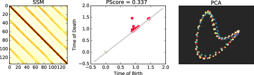
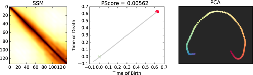
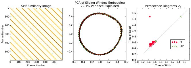
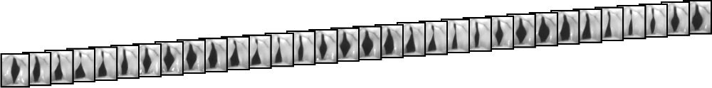
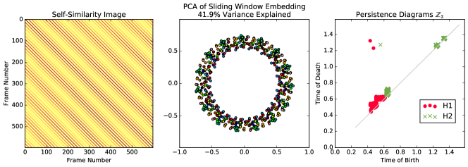
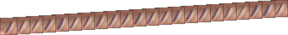
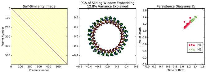
Results: We use a collection of 7 high-speed videos for this analysis, drawn from a variety of different sources [49], [26], [28], [13]. There are two videos which correspond to “normal” periodic vocal folds, three which correspond to biphonation [28], and two which correspond to irregular motion555Please refer to supplementary material for an example video from each of these three classes. We manually extracted 400 frames per video (100milliseconds) and autotuned the window size based on autocorrelation of 1D diffusion maps (Section 3.6). We then chose an appropriate and chose a time spacing so that each point cloud would have 600 points. As shown in Table 4, our technique is able to differentiate between the four classes. We also show PCA and persistence diagrams for one example for each class. In Figure 21, we see what appears to be a loop in PCA, and one strong 1D persistent dot confirms this. In Figure 22, we see a prominent torus in the persistence diagram. In Figure 23, we don’t see any prominent structures in the persistence diagram, even though PCA looks like it could be a loop or a torus. Note, however, that PCA only preserves 13.7% of the variance in the signal, which is why high dimensional techniques are important to draw quantitative conclusions.
| Video Name | Win | PS | MPS | QPS |
|---|---|---|---|---|
| Periodic 1 ([13]) | 16 | 0.816 | 0.789 | 0.011 |
| Periodic 2 ([26], Figure 21) | 32 | 0.601 | 0.533 | 0.009 |
| Biphonation 1 ([28]) | 53 | 0.638 | 0.294 | 0.292 |
| Biphonation 2 ([28]) | 42 | 0.703 | 0.583 | 0.116 |
| Biphonation 3 ([28], Figure 22) | 67 | 0.515 | 0.076 | 0.426 |
| Mucus Perturbed Periodic ([49]) | 94 | 0.028 | 0.019 | 0.004 |
| Irregular ([13], Figure 23) | 232 | 0.18 | 0.097 | 0.04 |
5 Discussion
We have shown in this work how applying sliding window embeddings to videos can be used to translate properties of the underlying dynamics into geometric features of the resulting point cloud representation. Moreover, we also showed how topological/geometric tools such as persistence homology can be leveraged to quantify the geometry of these embeddings. The pipeline was evaluated extensively showing robustness to several noise models, high quality in the produced periodicity rankings and applicability to the study of speech conditions form high-speed video data.
Moving forward, an interesting avenue related to medical applications is the difference between biphonation which occurs from quasiperiodic modes and biphonation which occurs from harmonic modes. [31] shows that field coefficients can be used to indicate the presence of a strong harmonic, so we believe a geometric approach is possible. This could be used, for example, to differentiate between subharmonic anomalies and quasiperiodic transitions [44].
Acknowledgments
The authors would like to thank Juergen Neubauer, Dimitar Deliyski, Robert Hillman, Alessandro de Alarcon, Dariush Mehta, and Stephanie Zacharias for providing videos of vocal folds. We also thank Matt Berger at ARFL for discussions about sliding window video efficiency, and we thank the 15 anonymous workers on the Amazon Mechanical Turk who ranked periodic videos.
References
- [1] Mark Allmen and Charles R Dyer. Cyclic motion detection using spatiotemporal surfaces and curves. In Pattern Recognition, 1990. Proceedings., 10th International Conference on, volume 1, pages 365–370. IEEE, 1990.
- [2] John Atanbori, Peter Cowling, John Murray, Belinda Colston, Paul Eady, Dave Hughes, Ian Nixon, and Patrick Dickinson. Analysis of bat wing beat frequency using fourier transform. In International Conference on Computer Analysis of Images and Patterns, pages 370–377. Springer, 2013.
- [3] Ulrich Bauer. Ripser: a lean C++ code for the computation of Vietoris–Rips persistence barcodes. http://ripser.org, 2015–2017.
- [4] Ronald R Coifman and Stéphane Lafon. Diffusion maps. Applied and computational harmonic analysis, 21(1):5–30, 2006.
- [5] Matthew JC Crump, John V McDonnell, and Todd M Gureckis. Evaluating amazon’s mechanical turk as a tool for experimental behavioral research. PloS one, 8(3):e57410, 2013.
- [6] Ross Cutler and Larry S. Davis. Robust real-time periodic motion detection, analysis, and applications. IEEE Transactions on Pattern Analysis and Machine Intelligence, 22(8):781–796, 2000.
- [7] Alain De Cheveigné and Hideki Kawahara. Yin, a fundamental frequency estimator for speech and music. The Journal of the Acoustical Society of America, 111(4):1917–1930, 2002.
- [8] Mauricio Delbracio and Guillermo Sapiro. Removing camera shake via weighted fourier burst accumulation. IEEE Transactions on Image Processing, 24(11):3293–3307, 2015.
- [9] Dimitar D Deliyski, Pencho P Petrushev, Heather Shaw Bonilha, Terri Treman Gerlach, Bonnie Martin-Harris, and Robert E Hillman. Clinical implementation of laryngeal high-speed videoendoscopy: challenges and evolution. Folia Phoniatrica et Logopaedica, 60(1):33–44, 2007.
- [10] Roman Goldenberg, Ron Kimmel, Ehud Rivlin, and Michael Rudzsky. Behavior classification by eigendecomposition of periodic motions. Pattern Recognition, 38(7):1033–1043, 2005.
- [11] Jerry P Gollub and Harry L Swinney. Onset of turbulence in a rotating fluid. Physical Review Letters, 35(14):927, 1975.
- [12] Allen Hatcher. Algebraic topology. University Press Ltd., 2002.
- [13] Christian T Herbst, Jakob Unger, Hanspeter Herzel, Jan G Švec, and Jörg Lohscheller. Phasegram analysis of vocal fold vibration documented with laryngeal high-speed video endoscopy. Journal of Voice, 30(6):771–e1, 2016.
- [14] Hanspeter Herzel, David Berry, Ingo R Titze, and Marwa Saleh. Analysis of vocal disorders with methods from nonlinear dynamics. Journal of Speech, Language, and Hearing Research, 37(5):1008–1019, 1994.
- [15] Hanspeter Herzel, Robert Reuter, and Richard A Katz. Biphonation in voice signals. In AIP Conference Proceedings, volume 375, pages 644–657. AIP, 1996.
- [16] Peng Huang, Adrian Hilton, and Jonathan Starck. Shape similarity for 3d video sequences of people. International Journal of Computer Vision, 89(2-3):362–381, 2010.
- [17] Shiyao Huang, Xianghua Ying, Jiangpeng Rong, Zeyu Shang, and Hongbin Zha. Camera calibration from periodic motion of a pedestrian. In Proceedings of the IEEE Conference on Computer Vision and Pattern Recognition, pages 3025–3033, 2016.
- [18] Xiaoye Jiang, Lek-Heng Lim, Yuan Yao, and Yinyu Ye. Statistical ranking and combinatorial hodge theory. Mathematical Programming, 127(1):203–244, 2011.
- [19] Holger Kantz and Thomas Schreiber. Nonlinear time series analysis, volume 7. Cambridge university press, 2004.
- [20] Maurice G Kendall. A new measure of rank correlation. Biometrika, 30(1/2):81–93, 1938.
- [21] Matthew B Kennel, Reggie Brown, and Henry DI Abarbanel. Determining embedding dimension for phase-space reconstruction using a geometrical construction. Physical review A, 45(6):3403, 1992.
- [22] Orrawan Kumdee and Panrasee Ritthipravat. Repetitive motion detection for human behavior understanding from video images. In Signal Processing and Information Technology (ISSPIT), 2015 IEEE International Symposium on, pages 484–489. IEEE, 2015.
- [23] Ofir Levy and Lior Wolf. Live repetition counting. In Proceedings of the IEEE International Conference on Computer Vision, pages 3020–3028, 2015.
- [24] Jörg Lohscheller, Hikmet Toy, Frank Rosanowski, Ulrich Eysholdt, and Michael Döllinger. Clinically evaluated procedure for the reconstruction of vocal fold vibrations from endoscopic digital high-speed videos. Medical image analysis, 11(4):400–413, 2007.
- [25] Philip Mcleod and Geoff Wyvill. A smarter way to find pitch. In In Proceedings of the International Computer Music Conference (ICMC’05, pages 138–141, 2005.
- [26] Daryush D Mehta, Dimitar D Deliyski, Thomas F Quatieri, and Robert E Hillman. Automated measurement of vocal fold vibratory asymmetry from high-speed videoendoscopy recordings. Journal of Speech, Language, and Hearing Research, 54(1):47–54, 2011.
- [27] George A Miller. The magical number seven, plus or minus two: some limits on our capacity for processing information. Psychological review, 63(2):81, 1956.
- [28] Jürgen Neubauer, Patrick Mergell, Ulrich Eysholdt, and Hanspeter Herzel. Spatio-temporal analysis of irregular vocal fold oscillations: Biphonation due to desynchronization of spatial modes. The Journal of the Acoustical Society of America, 110(6):3179–3192, 2001.
- [29] Sourabh A Niyogi, Edward H Adelson, et al. Analyzing and recognizing walking figures in xyt. In CVPR, volume 94, pages 469–474, 1994.
- [30] Jose A Perea. Persistent homology of toroidal sliding window embeddings. In Acoustics, Speech and Signal Processing (ICASSP), 2016 IEEE International Conference on, pages 6435–6439. IEEE, 2016.
- [31] Jose A Perea and John Harer. Sliding windows and persistence: An application of topological methods to signal analysis. Foundations of Computational Mathematics, 15(3):799–838, 2015.
- [32] Mark A Pinsky. Introduction to Fourier analysis and wavelets, volume 102. American Mathematical Soc., 2002.
- [33] Aaron M Plotnik and Stephen M Rock. Quantification of cyclic motion of marine animals from computer vision. In OCEANS’02 MTS/IEEE, volume 3, pages 1575–1581. IEEE, 2002.
- [34] Ramprasad Polana and Randal C Nelson. Detection and recognition of periodic, nonrigid motion. International Journal of Computer Vision, 23(3):261–282, 1997.
- [35] Qingjun Qiu, HK Schutte, Lide Gu, and Qilian Yu. An automatic method to quantify the vibration properties of human vocal folds via videokymography. Folia Phoniatrica et Logopaedica, 55(3):128–136, 2003.
- [36] Christian Schuldt, Ivan Laptev, and Barbara Caputo. Recognizing human actions: a local svm approach. In Pattern Recognition, 2004. ICPR 2004. Proceedings of the 17th International Conference on, volume 3, pages 32–36. IEEE, 2004.
- [37] Steven M Seitz and Charles R Dyer. View-invariant analysis of cyclic motion. International Journal of Computer Vision, 25(3):231–251, 1997.
- [38] Floris Takens. Detecting strange attractors in turbulence. In Dynamical systems and turbulence, Warwick 1980, pages 366–381. Springer, 1981.
- [39] Christopher Tralie. High-dimensional geometry of sliding window embeddings of periodic videos. In LIPIcs-Leibniz International Proceedings in Informatics, volume 51. Schloss Dagstuhl-Leibniz-Zentrum fuer Informatik, 2016.
- [40] Matthew Turk and Alex Pentland. Eigenfaces for recognition. Journal of cognitive neuroscience, 3(1):71–86, 1991.
- [41] Mikael Vejdemo-Johansson, Florian T Pokorny, Primoz Skraba, and Danica Kragic. Cohomological learning of periodic motion. Applicable Algebra in Engineering, Communication and Computing, 26(1-2):5–26, 2015.
- [42] V Venkataraman and P Turaga. Shape descriptions of nonlinear dynamical systems for video-based inference. IEEE transactions on pattern analysis and machine intelligence, 2016.
- [43] Ping Wang, Gregory D Abowd, and James M Rehg. Quasi-periodic event analysis for social game retrieval. In Computer Vision, 2009 IEEE 12th International Conference on, pages 112–119. IEEE, 2009.
- [44] Inka Wilden, Hanspeter Herzel, Gustav Peters, and Günter Tembrock. Subharmonics, biphonation, and deterministic chaos in mammal vocalization. Bioacoustics, 9(3):171–196, 1998.
- [45] Thomas Wittenberg, Manfred Moser, Monika Tigges, and Ulrich Eysholdt. Recording, processing, and analysis of digital high-speed sequences in glottography. Machine vision and applications, 8(6):399–404, 1995.
- [46] Or Yair, Ronen Talmon, Ronald R Coifman, and Ioannis G Kevrekidis. No equations, no parameters, no variables: data, and the reconstruction of normal forms by learning informed observation geometries. arXiv preprint arXiv:1612.03195, 2016.
- [47] Jing Yang, Hong Zhang, and Guohua Peng. Time-domain period detection in short-duration videos. Signal, Image and Video Processing, 10(4):695–702, 2016.
- [48] Guoshen Yu, Guillermo Sapiro, and Stéphane Mallat. Solving inverse problems with piecewise linear estimators: From gaussian mixture models to structured sparsity. IEEE Transactions on Image Processing, 21(5):2481–2499, 2012.
- [49] Stephanie RC Zacharias, Charles M Myer, Jareen Meinzen-Derr, Lisa Kelchner, Dimitar D Deliyski, and Alessandro de Alarcón. Comparison of videostroboscopy and high-speed videoendoscopy in evaluation of supraglottic phonation. Annals of Otology, Rhinology & Laryngology, page 0003489416656205, 2016.
- [50] A. Zomorodian and G. Carlsson. Computing persistent homology. Discrete & Computational Geometry, 33(2):249–274, 2005.