Describing dynamical fluctuations and genuine correlations by Weibull regularity

Abstract

The Weibull parametrization of the multiplicity distribution is used to describe the multidimensional local fluctuations and genuine multiparticle correlations measured by OPAL in the large statistics $\mbox{$e^{+}e^{-}$}\to Z^{0}\to{hadrons}$ sample. The data are found to be well reproduced by the Weibull model up to higher orders. The Weibull predictions are compared to the predictions by the two other models, namely by the negative binomial and modified negative binomial distributions which mostly failed to fit the data. The Weibull regularity, which is found to reproduce the multiplicity distributions along with the genuine correlations, looks to be the optimal model to describe the multiparticle production process.

1 Introduction

The understanding of multiparticle production in high-energy collisions is of high ineterest, as, on the one hand, its characteristics are immediate observables to provide important information on strong interactions, while, on the other hand, this process still faces difficulties in its complete understanding by the theory of strong interactions, Quantum Chromodynamics (QCD). The multiplicity of hadrons produced in high-energy collisions is one of the most straightforward measurements and provides a basic information about the dynamics of multiparticle production. Whereas the full-multiplicity distribution is a global characteristics of the events and is influenced by the conservation laws, the multiplicities averaged over the restricted phase-space regions (bins), or local multiplicity fluctuations, are less affected by the global constraints. These fluctuations combine contributions of multiparticle correlations which contain crucial information on the details of multihadron production mechanisms [1, 2, 3, 4, 5].

The local fluctuations have already attracted high interest and have been extensively studied using the method of the normalized factorial moments [1, 3]. The moments were proposed to extract the dynamical, non-Poissonian, fluctuations which were shown to lead to the effect called intermittency [6]. The intermittency effect shows itself as an increase of the factorial moments with decrease of the phase-space bin size (intermittency scaling). The intermittency phenomenon has been searched for in all types of collisions – from leptonic to nuclear ones – and it was observed to be a general feature of the multiparticle production process. The characteristics of multihadron production such as (multi)fractality (self-similarity) and different phase transition types associated with the intermittency have been widely investigated [1, 2, 3, 4].

The dynamical fluctuations contain a contribution not only of correlations but also from groups of uncorrelated particles. Then, the genuine correlations are mixed up in the fluctuations preventing us to reveal the dynamical features of the particle production process. To extract the genuine correlations, the method of the normalized factorial cumulant moments (cumulants) needs to be applied [7]. The cumulants are constructed from the $q$-particle ($q$th-order) cumulant correlation functions which vanish whenever one of their arguments becomes independent of the others [8], so that they measure the genuine correlations. The factorial cumulants remove the influence of the statistical component of the correlations in the same way as the factorial moments do. Employing an advantage of the method to search for many-particle correlations, the studies of the high-order ($q\geq 4$) genuine correlations have been performed in different types of collisions and reveal important features [1, 2, 3]. For example, the studies showed that the correlations in nuclear collisions are limited by the two-particle correlations while in $e^{+}e^{-}$ annihilations the important role of the higher-order correlations are obtained, the explanation of which was found in the many-source dilution effect [9]. It was also observed [1] that Monte Carlo models which reproduce well the single-particle distributions, fail to describe the measurements of the factorial moments and cumulants.

A general belief is that the local fluctuations stem from a generalized random cascade process involved in the particle production [10] or from branching processes in jet formation [11]. This is why one would expect the intermittency scaling of the moments (and cumulants) in $e^{+}e^{-}$ annihilation to be reproduced by the models based on the QCD parton shower with its inherent self-similarity. Being a sequential branching process, the parton cascade forms an integral part of the perturbative phase and it was also considered to play a significant role in the multiparticle production in $e^{+}e^{-}$ interactions. However, the QCD-based calculations are found to deviate from the measurements [12, 13] indicating a possible contribution of additional mechanisms to the transition from the perturbative partonic phase to the observed hadrons. Indeed, the Monte Carlo studies demonstrate [1] that the intermittency scaling manifesting itself at the level of the partonic shower is much weaker than that at the hadronic stage or is smeared out by the hadronization.

The branching feature of the intermittency has earlier been employed [14] by applying different parametrizations of the multiplicity distributions to the factorial and cumulant moments, measured by OPAL [15] in the high-statistics $e^{+}e^{-}$ annihilation data sample. The parametrizations which are most popular in multiparticle high-energy physics have been used, namely, the negative binomial (NB) distribution, its modified (MNB) and generalized forms, the log-normal (LN) distribution and the model pure-birth process with immigration (PB). Special attention has been devoted to the high-order cumulants ($q$ up to 5), the only higher-order cumulants measured at LEP. It is found that the LN and PB parametrizations fail to describe the data, overestimating or underestimating the measurements, respectively. The NB and MNB distributions are found to underestimate the data starting from the intermediate-size bins with the MNB spectra found to be closer to the measurements. The generalized NB distribution is found to show quite a complex behaviour due to different possible fitting areas of its two parameters, while demonstrates the behaviour similar to the NB and LN to which it reduces for special values of the parameters. Let us stress that the NB, LN and PB parametrizations are based on one parameter which is obtained from the second-order moments. That is, all the higher-order moments are based on the two-particle correlations and, therefore, the deviations of the predictions indicate the presence and importance of high-order correlations. This confirms the conclusion made in the measurements [15] by using the expansion of factorial moments by cumulants truncated to lower-order terms. The MNB has three parameters connected by a condition. In this case, the parameters were obtained from the second and third order moments, while the predictions were found to underestimate the higher-order moments indicating the inherent high-order correlations in the data.

The parametrizations considered in [14] are known to fail to describe the data on the full-phase-space multiplicity distribution with increasing energy, and the correlation study [14] elucidates a reason of this failure. For example, the discrepancy between the measured high-order correlations and the corresponding NB predictions [14, 16] points at an inadequacy of the single-NB to describe high-multiplicity tails in the multiplicity distribution, so, the high-order fluctuations. This would explain a need for a combination of two or more NB regularities [17] or its modification [18] and generalizations [19] to reproduce the multiplicity spectra (see [1, 5, 20] for reviews).

In this paper, we apply the Weibull parametrization of the multiplicity distribution. The Weibull distribution [21] is known to be a natural outcome of complex processes where cascading and sequential branching were involved [22]. In this sense, one would expect the Weibull distribution to be a natural candidate to describe the trend of the intermittency scaling. Moreover, in contrast to the parametrizations studied in [14], the Weibull regularity has been found [23] to describe well the multiplicity distributions in different types of collisions and at different energies. Recently, it was observed that the Weibull model is extremely successful in characterizing the multiplicity distributions (in the full phase-space and in its central rapidity intervals) up to the top LEP energies in $e^{+}e^{-}$ annihilations [24] and up to the TeV LHC energies in hadronic collisions [25]. Interestingly, the Weibull distribution is shown [24] to bridge the multiplicity distributions in $e^{+}e^{-}$ and $p\bar{p}$ interactions pointing at the multiparticle production universality as the dissipating effective-energy approach [26] considers it.

2 Weibull distribution, normalized factorial moments and cumulants

The Weibull distribution is a two-parameter distribution of a random variable $n$,

$$P(n,\lambda,\nu)=\frac{\nu\,n^{\nu-1}}{\lambda^{\nu}}\exp\left[-\left(\frac{n}{\lambda}\right)^{\nu}\,\right]$$

with the scale parameter $\nu>0$ and the shape parameter $\lambda>0$, and the mean

$$\langle n\rangle=\lambda\,\Gamma\!\left(\!1+\frac{1}{\nu}\right).$$

Here $\Gamma$ denotes the gamma function. The Weibull distribution reduces to the exponential distribution for $\nu=1$ and to the Rayleigh distribution for $\nu=2$.

For the normalized factorial moments, $F_{q}=\langle n(n-1)\cdots(n-q+1)\rangle/{\langle n\rangle}^{q}$, one finds:

$$F_{2}= \!\!\displaystyle\frac{1}{\lambda^{2}\,{\Gamma\!\left(\!1+\frac{1}{\nu}\right)}^{2}} \!\!\!\left\{-\lambda\,\Gamma\!\left(\!1+\frac{1}{\nu}\right)+\lambda^{2}\,\Gamma\!\left(\!1+\frac{2}{\nu}\right)\right\}\,,$$

$$F_{3}= \!\!\displaystyle\frac{1}{\lambda^{3}\,{\Gamma\!\left(\!1+\frac{1}{\nu}\right)}^{3}} \!\!\!\left\{2\,\lambda\,\Gamma\!\left(\!1+\frac{1}{\nu}\right)-3\,\lambda^{2}\,\Gamma\!\left(\!1+\frac{2}{\nu}\right)+\lambda^{3}\,\Gamma\!\left(\!1+\frac{3}{\nu}\right)\right\}\,,$$

$$\displaystyle F_{4}= \!\!\displaystyle\frac{1}{\lambda^{4}\,{\Gamma\!\left(\!1+\frac{1}{\nu}\right)}^{4}} \!\!\!\left\{-6\lambda\,\Gamma\!\left(\!1+\frac{1}{\nu}\right)+11\lambda^{2}\,\Gamma\!\left(\!1+\frac{2}{\nu}\right)-6\lambda^{3}\,\Gamma\!\left(\!1+\frac{3}{\nu}\right)\right.$$

$$\left.+\lambda^{4}\,\Gamma\!\left(\!1+\frac{4}{\nu}\right)\right\}\,,$$

$$F_{5}= \!\!\displaystyle\frac{1}{\lambda^{5}\,{\Gamma\!\left(\!1+\frac{1}{\nu}\right)}^{5}} \!\!\!\left\{24\lambda\,\Gamma\!\left(\!1+\frac{1}{\nu}\right)-50\lambda^{2}\,\Gamma\!\left(\!1+\frac{2}{\nu}\right)+35\lambda^{3}\,\Gamma\!\left(\!1+\frac{3}{\nu}\right)\right.$$ (1)

$$\left.-10\lambda^{4}\,\Gamma\!\left(\!1+\frac{4}{\nu}\right)+\lambda^{5}\,\Gamma\!\left(\!1+\frac{5}{\nu}\right)\right\}\,,\;\;\;{\rm etc.}$$

The factorial moments $F_{q}$ are related to the cumulants $K_{q}$ through the identities [1] (see also [2, 3, 5])

$$F_{q}=\sum_{m=0}^{q-1}{{q-1}\choose{m}}K_{q-m}\,F_{m}\,,$$

with $F_{0}=F_{1}=K_{1}=1$. For the first few orders the relations read

$$F_{2} \!\!\!= \!\!\!K_{2}+1\,,$$

$$F_{3} \!\!\!= \!\!\!K_{3}+3K_{2}+1\,,$$

$$F_{4} \!\!\!= \!\!\!K_{4}+4K_{3}+3K_{2}^{2}+6K_{2}+1\,,$$

$$F_{5} \!\!\!= \!\!\!K_{5}+5K_{4}+10K_{3}\,K_{2}+10K_{3}+15K_{2}^{2}+10K_{2}+1\,.$$ (2)

Calculating cumulants $K_{q}$ one extracts the genuine $q$-particle correlations. Note that thanks to the high statistics of the OPAL data, the uniformity of the measured single-particle distributions and the corrections made in [15], the translation invariance of the densities [27] is accounted for in the multiplicative terms in the expansions (2).

3 Comparison with measurements and discussion

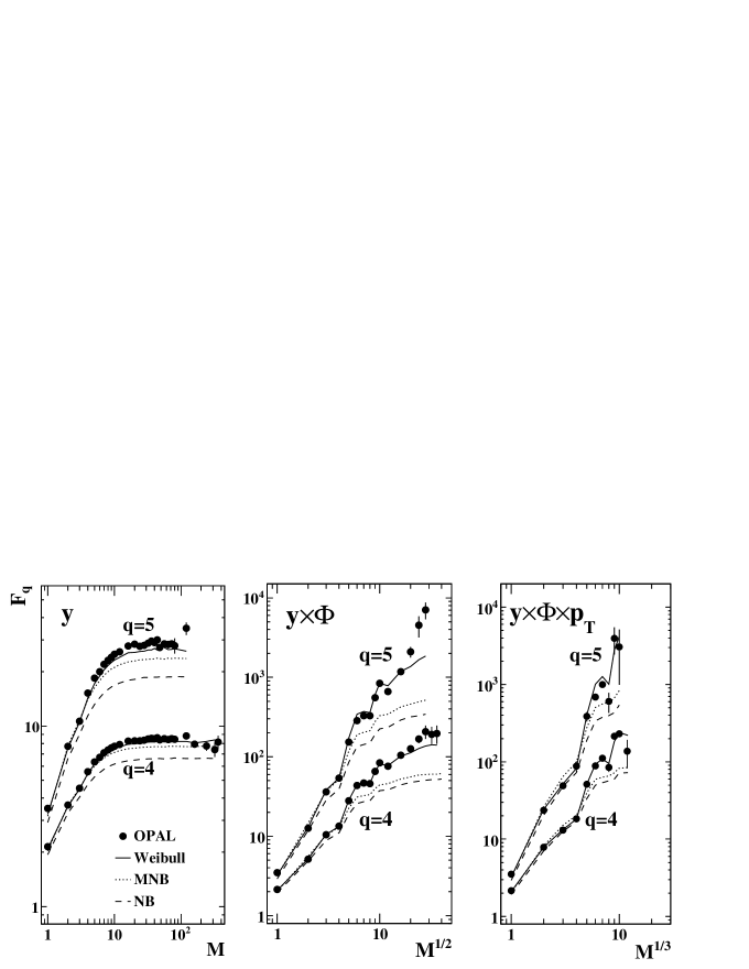
Figure 1: The normalized factorial moments of order $q=4$ and 5 as a function of $M^{1/D}$, where $M$ is the number of bins of the $D$-dimensional subspaces of the phase space of rapidity, azimuthal angle, and logarithm of transverse momentum, in comparison with the predictions of the Weibull, negative binomial (NB) and modified negative binomial (MNB) multiplicity parametrizations. The data are taken from [15]. The NB and MNB predictions are as in [14].

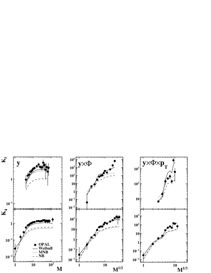
Figure 2: The normalized cumulants of order $q=4$ and 5 as a function of $M^{1/D}$, where $M$ is the number of bins of the $D$-dimensional subspaces of the phase space of rapidity, azimuthal angle, and logarithm of transverse momentum, in comparison with the predictions of the Weibull, negative binomial (NB) and modified negative binomial (MNB) multiplicity parametrizations. The data are taken from [15]. The NB and MNB predictions are as in [14].

Figures 1 and 2 show the normalized factorial moments and the normalized factorial cumulants, respectively, of the order $q>3$ measured by OPAL [15] in $e^{+}e^{-}$ annihilations and compared to a few parametrizations (lines). The moments are represented in one-, two- and three dimensions of the phase space of rapidity $y$, logarithm of the transverse momentum $p_{T}$ and azimuthal angle $\Phi$, calculated with respect to the sphericity axis. In addition to the Weibull predictions, the NB and MNB calculations from [14] are also given.

The NB predictions [28] use the measurements of the normalized factorial moments or cumulants of the second order to compute the NB $k$-parameter, $F_{2}-1=K_{2}=1/k$, and then the factorial moments and cumulants of order $q\geq 3$ are calculated according to the relations

$$F_{q}=\left(1+\frac{q-1}{k}\right)\,F_{q-1}$$

and

$$K_{q}=(q-1)!\,k^{1-q}\,.$$ (3)

From the comparison of the NB calculations with the data one can see that the calculations underestimate the measurements. Moreover, while the calculated $F_{q}$ moments deviate from the data starting from quite large $M$s (see Fig. 1), the cumulants clearly show the discrepancy already at small $M$-values (large bin sizes), see Fig. 2. The latter confirms that the genuine higher-order correlations are present in the data while contributing to the dynamical fluctuations along with the lower order correlations, which have been extracted by the cumulants in [15].

The MNB regularity leads to the following identities for the cumulants [18]:

$$K_{2}=K_{2}^{-}+\frac{1}{2\,k\,(r-\Delta)},\,\,\,K_{3}=K_{3}^{-}+\frac{K_{2}^{-}}{2\,k\,(r-\Delta)}\,,\,\,{\rm etc.},$$

with

$$K_{q}^{-}=(q-1)!\,k^{1-q}\,\frac{r^{q}-\Delta^{q}}{(r-\Delta)^{q}}\,,$$

where the superscript minus indicates cumulants for the negatively charged particles, and $r=\Delta+\langle n\rangle/k$. The MNB regularity reduces to the NB law if $\Delta=0$, c.f. Eq. (3). The factorial moments for the MNB regularity are calculated using the relations (2).

The MNB calculations are made based on the third order cumulants in the sense that the parameters $r$ and $\Delta$ have been fixed at the values $r=0.91$ and $\Delta=-0.71$, the best values found to describe at least the third-order cumulants [14]. Then the bin-size dependence is regulated by the only left parameter $k$, extracted from $K_{2}$ values. From the results of the MNB-based calculations, shown in Figs. 1 and 2, one concludes that the calculations are much closer to the data than those made with the NB regularity. However, even so, the MNB values underestimate the data for large $M$s (small bins), especially in two and three dimensions which points to the high-order genuine correlations not been large enough in the model.

The values of the normalized factorial moments based on the Weibull distributions, Eqs.(1), are shown in Fig. 1. The corresponding cumulants, shown in Fig. 2, are calculated using the relations (2). The parameters $k$ and $\lambda$ are estimated using the measurements of the second and third-order factorial moments.

From Fig. 1 one can see that the Weibull regularity describes well the measured factorial moments in one dimension of rapidity and in three dimensions, though one might notice discrepancy for the largest $M$ for $q=5$ in the $y$ subspace. The description is good as well in the two-dimensional $y\times\Phi$ subspace except a few extreme $M$ points for $q=5$, where the calculations give weaker fluctuations than those observed in the data. One can also see that the Weibull distribution gives much better description of the measurements compared to the NB and MNB distributions. Similarly, a good description is observed for the cumulants, as shown in Fig. 2. From these, one concludes that the Weibull regularity well reproduces not only the intermittency effect, i.e. the dynamical fluctuations combining genuine correlations of different order, but also the genuine high-order correlations.

4 Summary and conclusions

The Weibull distribution is used to describe the dynamical fluctuations and genuine high-order correlations of hadrons in restricted bins of the kinematic phase-space of $e^{+}e^{-}$ annihilation. The study exploits the high-statistics data of multidimensional normalized factorial moments and cumulants of charged particles measured by OPAL in $e^{+}e^{-}$ $\to Z^{0}$ hadronic decays. The Weibull parametrization, which earlier has been shown to well describe the multiplicity distribution in the wide range of the energy, is now found to well reproduce the measurements of multiplicity fluctuations and correlations in restricted bins of the phase space of rapidity, azimuthal angle and transverse momentum. The Weibull regularity is shown to provide much better description of the data compared to that given by other popular regularities such as the negative binomial and modified negative binomial distributions which mostly underestimate the data. This study further establishes that the Weibull distribution, which is found to be the first statistical model reproducing simulaneously the multiplicity distribution data and the data on the genuine multiparticle correlations, looks to be the optimal distribution to describe the multiparticle production process. The obtained results of the the Weibull calculations to successfully describe the crucial characteristics of the multihadron production such as genuine correlations, makes it of high interest to be applied to the measurements at LHC, where the Weibull model has already been shown to reproduce the multiplicity distributions in the full phase-space and in the central rapidity intervals. This is believed to cast new light on the hadroproduction process and to help to elucidate the predictions for the foreseen measurements at LHC, FCC and linear colliders.

Acknowledgements: S.D. thanks the Department of Science and Technology (DST), India, for partial support of this work. The work of M.T. is partially supported by the Projects LG15052 and LM2015058 of the Ministry of Education of the Czech Republic.

References

- [1] For review on correlations, intermittency and related topics in high-energy collisions, see: W. Kittel, E.A. De Wolf, Soft Multihadron Dynamics (World Scientific, Singapore, 2005).
- [2] P. Bozek, M. Ploszajczak, R. Botet, Phys. Rep. 252, 101 (1995).
- [3] E.A. De Wolf, I.M. Dremin, W. Kittel, Phys. Rep. 270, 1 (1996).
- [4] J. Manjavidze, A. Sissakian, Phys. Rep. 346, 1 (2001).
- [5] I.M. Dremin, J.W. Gary, Phys. Rep. 349, 301 (2001).
-
[6]
A. Białas, R. Peschanski,
Nucl. Phys. B 273, 703 (1986);
A. Białas, R. Peschanski, Nucl. Phys. B 308, 857 (1988), -
[7]
A.H. Mueller,
Phys. Rev. D 4, 150 (1971);
P. Carruthers, I. Sarcevic, Phys. Rev. Lett. 63, 1562 (1989). - [8] M.G. Kendall, A. Stuart, The Advanced Theory of Statistics, vol. 1 (C. Griffin, London, 1969).
-
[9]
G. Alexander, E.K.G. Sarkisyan,
Phys. Lett. B 487, 215 (2000);
G. Alexander, E.K.G. Sarkisyan, Nucl. Phys. B (Proc. Suppl.) 92, 21 (2001). - [10] A. Białas, K. Zalewski, Phys. Lett. B 228, 155 (1989).
- [11] W. Ochs, J. Wosiek, Phys. Lett. B 214, 617 (1988).
-
[12]
M. Acciarri et al., L3 Collaboration,
Phys. Lett. B 428, 186 (1998);
P. Abreau et al., DELPHI Collaboration, Phys. Lett. B 457, 368 (1999). - [13] G. Abbiendi et al., OPAL Collaboration, Phys. Lett. B 638, 30 (2006).
- [14] E.K.G. Sarkisyan, Phys. Lett. B 477, 1 (2000).
- [15] G. Abbiendi et al., OPAL Collaboration, Eur. Phys. J. C 11, 239 (1999).
- [16] G. Abbiendi et al., OPAL Collaboration, Phys. Lett. B 523, 35 (2001).
-
[17]
A. Giovannini, R. Ugoccioni,
Phys. Rev. D 59, 094020 (1999);
69, 059903 (2004) [Erratum];
A. Giovannini, R. Ugoccioni, Phys. Rev. D 68, 034009 (2003);
I.M. Dremin, V.A. Nechitailo, Phys. Rev. D 70, 034005 (2004);
I.M. Dremin, V.A. Nechitailo, Phys. Rev. D 84, 034026 (2011);
P. Ghosh, Phys. Rev. D 85, 054017 (2012);
I. Zborovský, J. Phys. G 40, 055005 (2013). -
[18]
P.V. Chliapnikov, O.G. Tchikilev,
Phys. Lett. B 242, 275 (1990);
N. Suzuki, M. Biyajima, N. Nakajima, Phys. Rev. D 53, 3582 (1996);
A. Capella, I.M. Dremin, V.A. Nechitailo, J. Tran Thanh Van, Z. Phys. C 75, 89 (1997). -
[19]
S. Hegyi,
Phys. Lett. B 387, 642 (1996);
G. Wilk, Z. Włodarczyk, J. Phys. G 44, 015002 (2017). - [20] J.F. Grosse-Oetringhaus, K. Reygers, J. Phys. G 37, 083001 (2010).
-
[21]
W. Weibull,
The Royal Swedish Institute of Engineering Research (Ingenors Vetenskaps
Akad. Handlingar), Proc. Nos. 151, 153, Stockholm, 1939;
W. Weibull, Nature 164, 1047 (1949);
W. Weibull, J. Appl. Mech. 18, 293 (1951). -
[22]
For review and discussion of the Weibull distribution, see:
W.K. Brown, J. Astrophys. Astron. 10, 89 (1989);
W.K. Brown, K.H. Wohletz, J. Appl. Phys. 78, 2758 (1995). -
[23]
S. Hegyi,
Phys. Lett. B 388, 837 (1996);
S. Hegyi, Phys. Lett. B 414, 210 (1997). - [24] S. Dash, B.K. Nandi, P. Sett, Phys. Rev. D 94, 074044 (2016).
- [25] S. Dash, B.K. Nandi, P. Sett, Phys. Rev. D 93, 114022 (2016).
-
[26]
E.K.G. Sarkisyan, A.S. Sakharov,
AIP Conf. Proc. 828, 35 (2006);
E.K.G. Sarkisyan, A.S. Sakharov, Eur. Phys. J. C 70, 533 (2010);
A.N. Mishra, R. Sahoo, E.K.G. Sarkisyan, A.S. Sakharov, Eur. Phys. J. C 74, 3147 (2014);
E.K.G. Sarkisyan, A.N. Mishra, R. Sahoo, A.S. Sakharov, Phys. Rev. D 93, 054046 (2016);
E.K.G. Sarkisyan, A.N. Mishra, R. Sahoo, A.S. Sakharov, Phys. Rev. D 94, 011501(R) (2016). - [27] P. Carruthers, H. Eggers, I. Sarcevic, Phys. Lett. B 254, 258 (1991).
-
[28]
B. Buschbeck, P. Lipa, R. Peschanski,
Phys. Lett. B 215, 788 (1988);
E.A. De Wolf, Acta Physica Polon. B 21, 611 (1990).