Abstract

Propagation of oscillatory signals through the cortex is shaped by the connectivity structure of neuronal circuits. The coherence of population activity at specific frequencies within and between cortical areas has been linked to laminar connectivity patterns. This study systematically investigates the network and stimulus properties that shape network responses. The results show how input to a cortical column model of the primary visual cortex excites dynamical modes determined by the laminar pattern. Stimulating the inhibitory neurons in the upper layer reproduces experimentally observed resonances at $\gamma$ frequency whose origin can be traced back to two anatomical sub-circuits. We develop this result systematically: Initially, we highlight the effect of stimulus amplitude and filter properties of the neurons on their response to oscillatory stimuli. Subsequently, we analyze the amplification of oscillatory stimuli by the effective network structure, which is mainly determined by the anatomical network structure and the synaptic dynamics. We demonstrate that the amplification of stimuli, as well as their visibility in different populations, can be explained by specific network patterns. Inspired by experimental results we ask whether the anatomical origin of oscillations can be inferred by applying oscillatory stimuli. We find that different network motifs can generate similar responses to oscillatory input, showing that resonances in the network response cannot, straightforwardly, be assigned to the motifs they emerge from. Applying the analysis to a spiking model of a cortical column, we characterize how the dynamic mode structure, which is induced by the laminar connectivity, processes external input. In particular, we show that a stimulus applied to specific populations typically elicits responses of several interacting modes. The resulting network response is therefore composed of a multitude of contributions and can therefore neither be assigned to a single mode nor do the observed resonances necessarily coincide with the intrinsic resonances of the circuit.

Author Summary

Oscillations are ubiquitously generated within and propagated between biological systems, for example in ecosystems, cell biology and the brain. Recordings from neural signals often show oscillations which are either generated within the recorded brain area or imposed on it from other areas. It is an open question in neuroscience how the underlying network structure influences the interaction between internally generated and externally applied oscillations. This study systematically analyzes how these two types of oscillations are reflected in the spectra produced by neural networks and whether oscillatory input can be utilized to uncover dynamically relevant sub-circuits of the neuronal network. Previous work showed that structured neural circuits yield dynamic modes which act as filters on internally generated noise of the neuronal activity. Here we show how these filters act on external input and how their superposition can yield resonances in the network response, which cannot directly be linked to the sub-circuits generating oscillations within the network. Simulation and theoretical analysis of a column model of the primary visual cortex show that oscillatory input applied to the inhibitory population in the upper layer elicits a resonance at $\gamma$ frequency in their response, which can be traced back to two distinct anatomical sub-circuits.

Introduction

Oscillations in the $\gamma$-frequency range ($30-80\,\mathrm{Hz}$) are observed ubiquitously in recordings of brain activity, such as the local field potential (LFP) [1, 2, 3]. On the single cell level, these oscillations can be generated from neurons with a preferred frequency at which they transmit signals. This band-pass filtering can arise from either single cell properties, for example sub-threshold resonances of cells which are driven by fluctuations [4], or from strongly driven cells whose input-output relation exhibits a peak at their firing rate [5]. On the network level, certain connectivity patterns have been hypothesized to facilitate very slow as well as fast oscillations in the $\gamma$-range [6], namely the inter-neuron $\gamma$ (ING) and pyramidal inter-neuron $\gamma$ (PING) motif (7, reviewed in 2). Although numerous theoretical studies shed light on the emergent behavior of theses dynamical motifs in isolation, few studies considered the effect of their embedment in larger networks, such as the layered structure of the cortex [8, 9]. Similarly, the dynamical interaction of the network motif with the surrounding network has been neglected when interpreting results of experimental studies gathering evidence for the ING motif [10] using oscillatory stimuli. In this study we analyze how the responses to oscillatory stimuli are shaped by the network alone and therefore only consider populations of neurons with non-resonant input-output relations.

Neural response properties [11, 12] as well as the emergence of oscillations in the $\gamma$-range [13] depend on the dynamical state of the network, which can be altered by externally applied stimuli. It is still a matter of debate which stimuli (natural or noise stimuli) elicit $\gamma$ oscillations [14, 15, 16] and whether $\gamma$ oscillations of different frequencies and peak shapes, elicited by these stimuli, are of the same anatomical origins [17, 15]. Changes of the excitability of neurons, that could be induced by stimuli, have theoretically been shown to have a strong impact on the oscillations generated within the network [18].

Probing the anatomical origin of network oscillations generated in the cortex has become more feasible since the emergence of optogenetic experiments [19, 20, 21], in which individual groups of neurons can be stimulated selectively. Evidence for $\gamma$ oscillations being generated by the interaction of inter-neurons alone has been gathered by means of periodic light stimulation in optogenetically altered mice [10]. A theoretical study [22] reproduces the experimental results by the analytical and numerical treatment of a network composed of excitatory and inhibitory neurons. The explanation requires gap junctions and a subthreshold resonance of the inhibitory neurons. Using Hodgkin-Huxley-type model neurons, Tiesinga [23] showed that the results of Cardin et al. can be reproduced by a PING mechanism if the excitatory cells have an additional slow hyperpolarizing current. This result strengthened the previous statement of the author [24] that experimental setups using oscillatory stimuli cannot distinguish between underlying ING and PING mechanisms.

We can summarize the difficulties that arise in the interpretation of these results with respect to the origin of the observed oscillations by three main points. First, it is still under debate how strongly external stimuli interfere with the dynamical state of the network. Histed et al. [25] pointed out that weak light impulses have a linear effect on the population responses of mice in vivo, which they found to be sufficiently predictive for changes in behavior. Second, mean-field theory of recurrent networks needs to be extended to incorporate oscillatory stimuli [24]. Third, the dynamical interaction of the connection pattern generating the oscillation with the surrounding network needs to be taken into account.

Describing oscillations that arise on the population level from weakly synchronized neurons, Ledoux et al. [26] investigate how external input shapes the dynamic transfer function, which describes the response of a neuron to small rate perturbations. However, they do not discuss the implications of this alteration for the dynamical properties to the population rate spectra in high-dimensional recurrently connected populations. Employing a similar framework, Barbieri et al. [27] showed by comparison to experimentally measured spectra that describing an input signal as a perturbation around the stationary state suffices to predict a considerable amount of the variance of the LFP.

In this work, population dynamics of spiking neurons are reduced to a rate-based description by a combined approach using mean-field theory to determine the stationary rates and linear response theory for the dynamical properties of the fluctuations. The reduction can therefore be understood as a two-step procedure. In the first step the stationary rate of the population is determined by evaluation of the nonlinear stationary transfer function [28, 29, 30], which depends on the mean and variance of the input to the population (also referred to as the working or operating point). All fluctuations around the working point are considered linear in the second step of the reduction, yielding the dynamic transfer function of the populations [31, 32, 33]. It has been shown that this level of reduction suffices to describe oscillations in neural networks, that are visible on the population but not on the single neuron level [34]. This reduction effectively maps the dynamics of each population composed of numerous neurons to a single noisy rate unit, which filters its input by a dynamic transfer function. Oscillations are therefore described as filtered noise (as found in [35]) and the neural network is reduced to coupled units, where the connections between the units shape the correlation structure of the network.

Keeping this reduction procedure in mind, we start from a rate based description to illustrate the phenomena that arise when considering oscillatory input to neural networks. In the first section, we use a negatively self-coupled population to analysize how different types of stimuli are reflected in different response measures. In particular, we consider large versus small and filtered versus non-filtered stimuli and their influence on absolute versus relative response spectra. In the second section, we study the contribution of the connectivity structure to the emergence and visibility of resonances in network responses by analyzing three characteristic network motifs composed of one excitatory and one inhibitory population each. Building on the insights gathered from low-dimensional coupled rate circuits analyzed in the first two sections, the third part is concerned with the analysis of resonances evoked by oscillatory stimuli in a microcircuit model based on primary sensory areas [36] comprising millions of spiking neurons.

We here show that phenomenological rate models with certain connectivity patterns suffice to explain resonance in the $\gamma$ range in response to oscillatory stimuli supplied to the inhibitory neurons, which is not visible when stimulating the excitatory neurons. In addition we demonstrate, that two different oscillation generating mechanisms, one involving only the inhibitory and one involving both the inhibitory and the excitatory neurons, generate similar resonances. In general terms, we show that the responses of sub-circuits in isolation are different than the responses of a system which embeds this sub-circuit. The fact that a complex system cannot be understood by the analysis of its parts in isolation, but only in its entirety has been pointed out before [37].

Results

Dynamic responses of a self-coupled inhibitory population

In this section, we analyze how input is processed in a negatively self-coupled dynamical rate unit that produces a rhythm in the $\gamma$-frequency range. The model is inspired by a population of inhibitory leaky-integrate-and-fire (LIF) neurons. We here contrast large versus small stimuli as well as stimuli that affect the input current to the unit versus the output rate of the unit. Changes induced by the input are considered in the spectrum as well as in the power ratio (the spectrum normalized by the spectrum without input).

A sketch of the circuit with and without input is depicted in Fig 1A. The dynamics of the circuit is determined by its dynamic transfer function, which we here choose to approximate the dynamics in a corresponding population of LIF neuron models with delays (for further detail see “Static and dynamic transfer function of LIF-neurons”) as

$$H(\omega)=\frac{A\,e^{-i\omega d}}{1+i\omega\tau}\,e^{-\frac{\sigma_{d}^{2}\omega^{2}}{2}}.$$ (1)

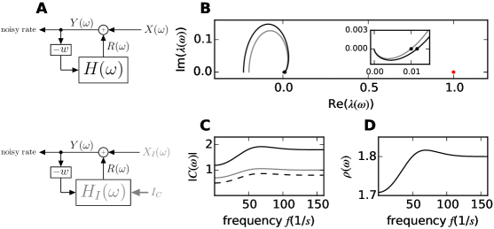
Figure 1: Dynamics of a self-coupled inhibitory population with constant stimulus. A upper sketch: default circuit (Eq (3)). The population characterized by the dynamic transfer function $H(\omega)$ emits the rate $R(\omega)$, which combined with the noise $X(\omega)$ yields the observed noisy rate $Y(\omega)$, which is amplified by $-w$ and fed back to the population. Lower sketch: circuit as above with additional constant input, which alters the dynamic transfer function and the variance of the noise. B Eigenvalue trajectories (Nyquist plot) $\lambda(\omega)=-wH(\omega)$ and $\lambda_{I}(\omega)=-wH_{I}(\omega)$ for the circuit with (black curve) and without (gray curve) additional constant input, respectively. The inset shows the values of the two trajectories for higher frequencies, where the solid black dots denote their closest approach to the value one. The close zoom shows that the eigenvalue trajectory assumes negative imaginary values before it converges to zero. C Spectrum of the circuit with ($C_{I}(\omega)$, black solid curve, Eq (5)) and without ($C(\omega)$, gray solid curve, eq. Eq (4)) additional constant input and their difference ($C_{I}(\omega)-C(\omega)$, dashed black curve). D Power ratio of the spectra with and without input $\rho(\omega)=C_{I}(\omega)/C(\omega)$. Parameters of the circuit are specified in Eq (49).

Here $\tau$ denotes the effective time constant of the dynamic transfer function and $A$ its amplitude in response to a constant current. The multiplicative factors $e^{-i\omega d}$ and $e^{-\frac{\sigma_{d}^{2}\omega^{2}}{2}}$ originate from the Gaussian distributed delays and with mean $d$ and variance $\sigma_{d}$. We here choose the variance equal to the mean, i.e. $\sigma_{d}=d$. The first factor promotes oscillations, while the second one suppresses the transfer of large frequencies. In multi-dimensional systems, the generation of each peak in the spectrum can be attributed to the dynamics of one eigenmode of the system, where the dynamic transfer function of the $i$-th eigenmode is given by the corresponding eigenvalue $\lambda_{i}(\omega)$ [34]. Each mode emerges from the interplay of several populations. The transfer function here could hence also be interpreted as the transfer function of one dynamic mode. In this case its parameters are understood as effective parameters, which are composed of the parameters of all populations contributing to this mode.

The observed rate $Y$ of the unit is given by its output rate $R(\omega)$ combined with additive white noise $X(\omega)$ with zero mean $\langle X(\omega)\rangle=0$ and non-zero variance $\langle X(\omega)X^{\mathrm{T}}(-\omega)\rangle=D$ as

$$Y(\omega)=R(\omega)+X(\omega).$$ (2)

The noise term originates from the fact that the considered rate profile actually describes a spike train. In other words, the spike train can be considered as a noisy realization of the rate profile $R(\omega)$. The internally generated noise in self-coupled populations of LIF neurons exhibits a variance of $D=\frac{r_{0}}{N}$ [38], where $r_{0}$ denotes the stationary rate of the neurons in the population and $N$ the number of neurons. The fluctuating rate produced by the circuit (Fig 1A upper sketch) reads

$$Y(\omega)=-wH(\omega)\,Y(\omega)+X(\omega)$$

$$\Leftrightarrow Y(\omega)=\frac{1}{1-\lambda(\omega)}X(\omega),$$ (3)

where the fed back rate is weighted by the feedback strength $-w$ and we identify $\lambda(\omega)=-wH(\omega)$ as the eigenvalue of the one-dimensional system. When considering LIF neuron models, the strength $w$ is determined by the synaptic amplitude and the number of connections. The spectrum of the population without additional input is given by

$$C(\omega)=\langle Y(\omega)Y^{\mathrm{T}}(-\omega)=\left|\frac{1}{1-\lambda(\omega)}\right|^{2}D.$$ (4)

Fig 1B shows the Nyquist plot of the eigenvalue $\lambda(\omega)$, which determines the shape of the spectrum. The peak frequency is determined by the point at which the eigenvalue trajectory assumes its closest distance to unity, resulting in a large prefactor in Eq (4) (see also [34]). The parameters of the dynamic transfer function (Eq (49)) are based on the dynamic transfer function of populations in a large scale model composed of LIF neurons [36] and chosen to produce a peak in the $\gamma$ frequency range (Fig 1C). The mapping between the LIF neurons and rate models is described in the first sections of the “Methods”.

When considering the effect of external input to the spectrum in the following, we distinguish weak and strong stimuli that require different levels of description: Large input changes the stationary rate and the dynamic properties of the population. Small input can be treated as a perturbation around the stationary point which itself remains unchanged. We will show in the last part of this study, that a small oscillatory component in the input to a population is sufficient to affect its spectrum considerably. We therefore neglect the effect of the oscillatory component of the stimulus onto the stationary point and restrict this analysis to either oscillatory input, which can be treated as a perturbation, or oscillatory input with an additional constant offset that may change the stationary state.

We start by applying a large constant input to the population, yielding an altered stationary rate of the system $r_{0}\rightarrow r_{0}+\delta r_{0}$. This changes the spectrum for two reasons. First, the dynamic properties of the population change yielding a new dynamic transfer function $H(\omega)\rightarrow H_{I}(\omega)$ ($\lambda(\omega)\rightarrow\lambda_{I}(\omega)$). This occurs in systems whose dynamic transfer function depends on the statistics of the input, which is also referred to as the working point. In general, an increase in the external rate can yield large changes in the dynamic transfer function. However, reasonably sized stimuli applied to populations in the fluctuation driven regime primarily affect the offset of the transfer function and leave the shape approximately unaltered (see “Approximation of the dynamic transfer function”). This suggests the following approximation $H_{I}(\omega)\approx(1+\delta A/A)\,H(\omega)$ (see Fig 1B for the shifted eigenvalue trajectory). Second, the input alters the stationary rate of the circuit and therefore the amplitude of the internally generated noise $D\rightarrow D_{I}=(r_{0}+\delta r_{0})/N$. The new spectrum is hence given by

$$C_{I}(\omega)=\left|\frac{1}{1-\lambda_{I}(\omega)}\right|^{2}D_{I}.$$ (5)

In the following $C_{I}(\omega)$ is termed the response spectrum, $\delta C(\omega)=C_{I}(\omega)-C(\omega)$ the excess spectrum, and $\rho(\omega)=\frac{C_{I}\omega)}{C(\omega)}$ the power ratio. The latter is commonly used in experimental studies since it is insensitive to the filtering of the local field potential by the extracellular tissue [39] and dendritic morphology [40], provided that both can be approximated as activity independent. All three measures display a peak at the frequency generated by the circuit (Fig 1C,D). The peak arises because the excitatory input provided to the system effectively strengthens the inhibitory loop that generates the oscillation by shifting the eigenvalue closer to the value one and therefore closer to a rate instability [34].

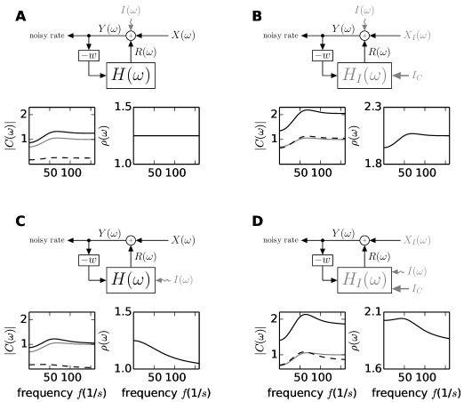
Figure 2: Dynamics of a self-coupled inhibitory population with oscillatory and constant stimuli. The four panels depict four different types of input for the circuit shown in Fig 1A. In each panel the top shows a sketch of the circuit. The bottom left panel shows the spectrum of the circuit at frequency $\omega$ without input ($C(\omega)$, gray solid curve, Eq (4)) and at stimulation frequency $\omega_{\mathrm{I}}$ with input ($C_{I}(\omega)$, black solid curve). Their difference ($C_{I}(\omega)-C(\omega)$) as a function of the stimulation frequency $\omega_{\mathrm{I}}$, is depicted by the dashed black curve. The bottom left panel shows the power ratio of the spectrum with and without input $\rho(\omega)=C_{I}(\omega)/C(\omega)$. Parameters of the circuit are specified in Eq (50). A Circuit subject to a periodic modulation of the rate $\propto I(\omega)$ (Eq (6)). The oscillatory input can be treated as a perturbation and therefore added to the internally generated noise. B Circuit subject to a periodic modulation of the rate $\propto I(\omega)$ and a large constant component $I_{C}$ (Eq (8)). The latter changes the dynamic transfer function and the variance of the noise. C Input current modulated circuit (Eq (6)). The oscillatory input is send through the population filter before entering the circuit. D Input current modulated circuit with a large constant component (Eq (8)), that changes the dynamic transfer function and the variance of the noise.

Oscillatory input current injected into a neuron is necessarily filtered by the dynamic transfer function of the neuron. It is, however, the change in population firing rate that is recurrently processed on the network level and eventually constitutes the measurable network response. To this end we compare network responses to two types of stimuli. The first type causes a modulation of the input current (“current modulation”, CM), and the second type directly modulates the output rate (“rate modulation”, RM, see also the illustrations in Fig 2B,C). In the first case the stimulus is filtered by the dynamic transfer function before it affects the activity of the population (see “Composition of the spectrum with input”), while it can be directly added to the rate in the latter case. The spectrum of the stimulated network hence reads

$$C_{I}(\omega) = \left|\frac{1}{1-\lambda(\omega)}\right|^{2}\Big{(}D+R_{\mathrm{I}}(\omega)R_{\mathrm{I}}^{*}(\omega)\Big{)}$$ (6)

$$\mbox{with\,\,}R_{\mathrm{I}}(\omega)=\begin{cases}I(\omega)&\mbox{for rate modulation (RM)}\\ H(\omega)I(\omega)&\mbox{for current modulation (CM).}\end{cases}$$

Here $I(\omega)$ describes the stimulus in Fourier domain. Experimental studies considered periodic stimuli to investigate the circuits underlying the generation of oscillations [10]. Supplying a sinusoidal stimulus with frequency $\omega_{I}$ ($I(\omega)=i\pi I_{0}\left(\delta(\omega+\omega_{I})-\delta(\omega-\omega_{I})\right)$) to the one-dimensional circuit contributes an additional term to the spectrum at stimulus frequency and yields the following power ratio

$$\rho(\omega)=\frac{C_{I}(\omega)}{C(\omega)}=1+\frac{1}{D}\begin{cases}\pi^{2}I_{0}^{2},&\mbox{\mbox{for rate modulation}}\\ \pi^{2}I_{0}^{2}\left|H(\omega)\right|^{2}&\mbox{for current modulation}\end{cases}\>\mbox{and}\>\omega=\omega_{I}.$$ (7)

This expression shows in particular, that the power ratio is independent of the resonance properties of the circuit, since its contributions (which are described in Eq (4)) cancel. The power ratio is independent of the stimulus frequency for rate modulated systems (Fig 2A), while it reflects the shape of the population filter $H$ in current modulated systems (Fig 2C). This tendency is also reflected in the response spectrum, which displays a constant offset in the RM system while for the CM system it approaches the spectrum without stimulus for higher frequencies due to the low-pass filter of the population.

This insight can be directly transferred to experimental studies. To investigate the anatomical origin of oscillations, one seeks to analyze the dynamics of the rate fluctuations generated within the circuit. Hence, an upstream low-pass filter can give the false impression that slow rate fluctuations are generated within the circuit, even though they arise from the filter of the population. Adjusting the input strength to emphasize fast frequencies can compensate for the low-pass filtering of the populations; to this end one needs to replace the amplitude as $I_{0}\rightarrow I_{0}/\left|H(\omega)\right|$. An exact experimental implementation of this protocol is only possible, if the dynamic transfer function of the stimulated neuronal population is known. However, the relation can still be employed in an approximate manner to counteract known influences. For example Tiesinga [23] modeled optogenetic stimuli as AMPA mediated currents. Since the dynamic transfer function is a convolution of the synaptic and the population filter, the synaptic filter could be counteracted in experiments by considering the underlying receptor and neurotransmitter density, which determine the time scales of the synaptic currents.

The two effects described above can be combined in a stimulus that has a constant component, which increases the susceptibility and firing rate of the target population, as well as an oscillatory component. This yields the following power ratios at $\omega=\omega_{I}$

$$\rho(\omega) = \left|\frac{1-\lambda(\omega)}{1-\lambda_{I}(\omega)}\right|^{2}\frac{D_{\mathrm{I}}+|I_{I}(\omega)|^{2}}{D}$$ (8)

$$= \left|\frac{1-\lambda(\omega)}{1-\lambda_{I}(\omega)}\right|^{2}\begin{cases}\Big{(}\frac{D_{\mathrm{I}}}{D}+\frac{I_{0}^{2}}{D}\Big{)}&\mbox{\mbox{for rate modulation}}\\ \Big{(}\frac{D_{\mathrm{I}}}{D}+\frac{I_{0}^{2}\left|H_{I}(\omega)\right|^{2}}{D}\Big{)}&\mbox{for current modulation.}\end{cases}$$

From the analysis of the spectrum with constant input and from Eq (5) we know that the constant component of the stimulus shifts the eigenvalue, such that the $\lambda$-dependent prefactor in the latter equation displays a peak close to the internally generated frequency. This peak, which reflects a positive change in the excitability of the population ($D_{\mathrm{I}}>D\Rightarrow H_{I}(0),\lambda_{\mathrm{I}}(0)>H(0),\lambda(0)$), is clearly visible in the rate modulated system (Fig 2B). Here, the frequency independent contribution of the oscillatory stimulus is added to the internal fluctuations. It therefore amplifies the peak, which is shaped by the shift in the working point, but it cannot affect the shape of the spectrum by itself. The spectrum for current-modulated circuits experiences additional amplification at low frequencies compared to the rate modulated circuit due to the multiplications of the dynamic transfer function. If the change in excitability is large, this amplification of low frequencies can overshadow the peak caused by the shift in working point. The balance between these two effects depends on the parameters of the population filter and the rise in excitability ($H_{I}(\omega)-H(\omega)$, for small $\omega$) compared to the closeness of the system to an instability, characterized by the term $\left|1-\lambda_{I}(\omega)\right|^{2}$(at peak frequency).

In summary, the analysis of a one-dimensional self-coupled population shows that the responses of the circuit can vary widely depending on the properties of the system and the stimulus. Namely, a stimulus that affects the stationary state of the system changes its dynamic properties and therefore alters the strength of internally generated oscillations. Stimuli that can be treated as perturbations amplify the internally generated oscillation, but do not change the underlying dynamical circuits that shape the spectrum. Input that directly affects the rate of the population reveals information regarding the dynamics of the circuit, while the responses to stimuli that are added to the input current to the population run the risk of reflecting the filter properties of the populations. These effects dominate the frequency-dependence of power ratios, which become independent of the resonance properties of the circuit. The response and the excess spectrum, in contrast, both exhibit peaks at the internally generated oscillation. It is therefore advantageous to consider one of the two latter quantities in addition to the power ratio.

Stimulus evoked spectra in a two dimensional network

In neural circuits, recurrent loops generating characteristic oscillations do not appear in isolation, but are embedded into larger networks. To analyze the effect of the surrounding network on the responses elicited by oscillatory stimuli, we start by considering oscillation generating circuits composed of one or two populations. We first describe how the oscillations generated within the network can be understood by means of dynamical modes and how the effect of a stimulus vector can be split into components that each excite a different mode. The responses of individual modes can in principal be traced back to an anatomical circuit that generates the oscillation. However, the identification of the origin of an oscillation is usually complicated by the fact that responses to stimuli are composed of multiple modes. To isolate this phenomenon we study three exemplary circuits in which evoked responses can be treated as perturbations. Here, applied stimuli modulate the rate directly (RM), assuming a stimulation protocol which counteracts the filter properties of the population that receives the input.

A two-dimensional circuit, as shown in Fig 3A, is composed of an excitatory (E) and an inhibitory (I) population, with the dynamic transfer functions of population $i$ receiving input from population $j$

$$H_{ij}(\omega)=\frac{A_{i}e^{-i\omega d_{j}}}{1+i\omega\tau_{i}}\,e^{-\frac{\sigma_{d_{j}}^{2}\omega^{2}}{2}},\>i,j\in{E,I},$$ (9)

where $d_{j}$ denotes the delay of a connection starting at population $j$. To illustrate the phenomena analyzed here in the simplest possible setup, we assume that the neurons in the two populations have equal working points and that the delays of all synapses are identically distributed. The neurons therefore have equal stationary firing rates $(r_{0,\mathrm{E}},r_{0,\mathrm{I}})=(r_{0},r_{0})$ as well as equal transfer functions $H_{ij}(\omega)=H(\omega)$. The connectivity matrix is given by

$$\mathbf{W}=\left(\begin{array}[]{cc}a&-b\\ c&-d\end{array}\right)$$ (10)

with all parameters being positive $a,\>b,\>c,\>d>0$. In networks of LIF-neuron models, these parameters are given by the product of in-degrees and connection strength ($a=w_{EE}K_{EE}$, $b=w_{EI}K_{EI}$, $c=w_{IE}K_{IE}$, and $d=w_{II}K_{II}$). The effective connectivity matrix, which combines the anatomical and dynamic properties of the circuit, is given by $\mathbf{M}(\omega)=H(\omega)\,\mathbf{W}$, with the eigenvalues

$$\tilde{\lambda}_{0,1}(\omega)=H(\omega)\underset{=\lambda_{0,1}}{\underbrace{\left(\frac{a-d}{2}\pm\sqrt{\frac{(a-d)^{2}}{4}-(bc-da)}\right)}.}$$ (11)

The right ($\boldsymbol{u}_{i}$) and left ($\boldsymbol{v}_{i}$) eigenvectors are given by

$$\mathbf{u}_{0}=\mathbf{v}_{0}=\left(\begin{array}[]{c}1\\ 0\end{array}\right),\>\mathbf{u}_{1}=\mathbf{v}_{1}=\left(\begin{array}[]{c}0\\ 1\end{array}\right)\quad\mbox{if}\>b=c=0$$ (12)

or

$$\mathbf{u}_{i}=\frac{1}{y_{i}}\left(\begin{array}[]{c}1\\ x_{i}\end{array}\right),\>\mathbf{v}_{0}=\frac{y_{0}}{x_{1}-x_{0}}\left(\begin{array}[]{c}x_{1}\\ -1\end{array}\right),\>\mathbf{v}_{1}=\frac{y_{1}}{x_{1}-x_{0}}\left(\begin{array}[]{c}-x_{0}\\ 1\end{array}\right)$$ (19)

$$\mbox{with}\>x_{i}=\begin{cases}\frac{a-\lambda_{i}}{b}&\mbox{if}\>c=0\\ \frac{c}{\lambda_{i}+d}&\mbox{else}\end{cases}\,\mbox{and}\,y_{i}=\sqrt{1+|x_{i}|^{2}}.$$ (20)

They are bi-orthogonal and normalized such that $|\mathbf{u}_{i}|^{2}=1$ and $\mathbf{v}_{i}^{\mathrm{T}}\mathbf{u}_{j}=\delta_{ij}$. Note that in a more general setting, where the populations have different stationary activities and therefore different transfer functions, the eigenvectors are frequency dependent. The spectrum produced by the circuit can be expressed as the sum of spectra produced by the eigenmodes due to their auto- ($n=m$) and their crosscorrelation ($n\neq m$) (see “Composition of the spectrum”)

$$\mathbf{C}(\omega)=\sum_{n,m\in\{0,1\}}\frac{\beta_{nm}}{(1-\tilde{\lambda}_{n}(\omega))(1-\tilde{\lambda}_{m}^{*}(\omega))}\mathbf{u}_{n}\mathbf{u}_{m}^{\mathrm{T}*}$$ (21)

with $\beta_{nm}=\sum_{i}D_{ii}\alpha_{n}^{i}\alpha_{m}^{i}$, where $\alpha_{j}^{i}=\mathbf{v}_{j}^{\mathrm{T}}\mathbf{e}_{i}$ denotes the projection of the $j$-th left eigenvector onto the $i$-th unit vector with $\mathbf{e}_{i}^{\mathrm{T}}\in\left\{(\begin{array}[]{cc}1,&0\end{array}),(\begin{array}[]{cc}0,&1\end{array})\right\}$. For LIF neuron models the diagonal elements of the stationary activity matrix are given by $D_{ii}=r_{0,i}/N_{i}$. When describing neuronal populations, the auto- and crosscorrelations of the modes describe properties of groups of neurons, namely the summed correlations on the single neuron level. For example, the autocorrelation of one modes refers to the sum of all auto- and crosscorrelations between neurons that constitute that mode.

The diagonal elements of $\mathbf{C}(\omega)$ (Eq (21)) describe the spectra of the population activity. For frequencies $\omega_{c}$ at which one eigenvalue $\tilde{\lambda}_{c}(\omega_{c})$ approaches the value one, a peak is visible in the spectrum. The anatomical connections that determine the amplitude and frequency of this peak can be established using the following quantities [34]

$$Z_{ij}^{\mathrm{amp}}=\left(\Re(Z_{ij}),\Im(Z_{ij})\right)\mathbf{k}^{\mathrm{T}}\quad\mbox{and}\quad Z_{ij}^{\mathrm{freq}}=\left(\Re(Z_{ij}),\Im(Z_{ij})\right)\mathbf{k}_{\perp}^{\mathrm{T}},$$ (22)

which identify the sensitivity of the eigenvalue to the connections (defined by the matrix elements $M_{ij}$) via

$$Z_{kl}=\frac{v_{c,k}M_{kl}u_{c,l}}{\mathbf{v}_{c}^{\mathrm{T}}\mathbf{u}_{c}},$$ (23)

where $\mathbf{u}_{c}$ and $\mathbf{v}_{c}$ are the right and left eigenvector associated to $\lambda_{c}(\omega_{c})$. The unit vectors that describe directions in the complex plane: $\mathbf{k}$ points from $\lambda_{c}(\omega)$ to the one and $\mathbf{\mathbf{k}_{\perp}}$ perpendicular to $\mathbf{\mathbf{k}}$, are given by

$$\mathbf{k} =(1-\Re(\lambda_{c}),\Im(\lambda_{c}))/\sqrt{(1-\Re(\lambda_{c}))^{2}+\Im(\lambda_{c})^{2}}$$

$$\mathbf{k}_{\perp} =(-\Im(\lambda_{c}),1-\Re(\lambda_{c}))/\sqrt{(1-\Re(\lambda_{c}))^{2}+\Im(\lambda_{c})^{2}},$$ (24)

where all dependencies on frequency were omitted for brevity of notation.

In electrophysiological recordings, the activities of the excitatory and the inhibitory population are often indirectly observed via the local field potential (LFP), which has been related to the input of pyramidal neurons [41] (see “Approximation of the LFP”)

$$C_{\mathrm{LFP}}(\omega)=\underset{:=C_{\mathrm{LFP}}^{\mathrm{auto}}(\omega)}{\underbrace{a^{2}C_{\mathrm{E}\mathrm{E}}(\omega)+b^{2}C_{\mathrm{I}\mathrm{I}}(\omega)}}+\underset{:=C_{\mathrm{LFP}}^{\mathrm{cross}}(\omega)}{\underbrace{2ab\Re\left(C_{\mathrm{E}I}(\omega)\right)}}.$$ (25)

The LFP gets contributions from the excitatory and the inhibitory current onto the excitatory neurons as well as from their crosscorrelation. Defining the LFP in this way implicitly assumes $\delta$-shaped synaptic currents, otherwise the contributions above would additionally be filtered by the synaptic kernels (see Eq (79)). Stimulating the circuit with sinusoidal input $F(\omega)=i\pi I_{0}\left[\delta(\omega+\omega_{I})-\delta(\omega-\omega_{I})\right]$ of frequency $\omega_{I}$ and amplitude $I_{0}$ in the direction $\mathbf{e}_{I}$ elicits the excess spectrum (see Eq (77)) at $\omega=\omega_{I}$

$$\delta\mathbf{C}(\omega)=\mathbf{C}_{I}(\omega)-\mathbf{C}(\omega)=\sum_{n,m\in\{0,1\}}\underset{=\delta\mathbf{C}^{nm}(\omega)}{\underbrace{\frac{\beta_{nm}^{I}}{(1-\tilde{\lambda}_{n}(\omega))(1-\tilde{\lambda}_{m}^{*}(\omega))}\mathbf{u}_{n}\mathbf{u}_{m}^{\mathrm{T}*}}}$$ (26)

with $\beta_{nm}^{I}=\pi^{2}I_{0}^{2}\gamma_{n}\gamma_{m}^{*}$, where $\gamma_{j}=\mathbf{v}_{j}^{\mathrm{T}}\mathbf{e}_{I}$ marks the projection of the stimulus direction onto the left eigenvector. If the stimulus vector is parallel to the right eigenvector of one mode $\mathbf{e}_{I}=x\mathbf{u}_{k}$ it will excite only this mode ($\gamma_{k}=x,\,\gamma_{i\neq k}=0$). The scalar $\gamma_{i}$ therefore measures the portion by which the $i$-th eigenmode is stimulated by the stimulus vector $\mathbf{e}_{I}$. The stimulus-induced component of the LFP response that originates in the autocorrelation of the currents is given by

$$\delta C_{\mathrm{LFP}}^{\mathrm{auto}}(\omega)=C_{\mathrm{LFP},I}^{\mathrm{auto}}(\omega)-C_{\mathrm{LFP}}^{\mathrm{auto}}(\omega)=\sum_{n,m\in\{0,1\}}\left(a^{2}\delta C_{\mathrm{E}\mathrm{E}}^{nm}(\omega)+b^{2}\delta C_{\mathrm{I}\mathrm{I}}^{nm}(\omega)\right).$$ (27)

Since the contributions of individual modes are more straightforward to separate for the autocorrelations, we only consider the LFP contribution defined in Eq (27) in detail (see Eq (79) for the full LFP spectrum). It will, however, be shown, that the crosscorrelations do not interfere with the discussed effects.

In the following sub-sections, we will show on three exemplary circuits, that non-negligible connectivity between populations evokes responses of several modes when individual populations are stimulated. The interference of these mode responses can yield similar network responses for different underlying network structures.

A self-coupled inhibitory circuit embedded in a two-dimensional network

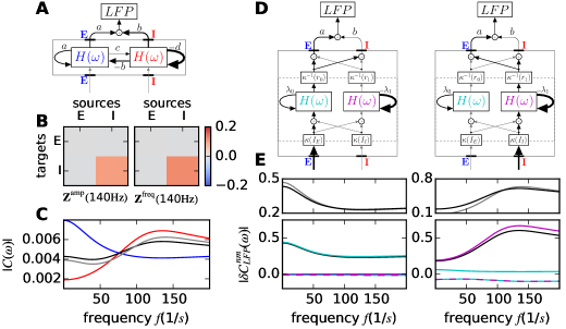
Figure 3: Responses of a circuit with an embedded self-coupled inhibitory population to oscillatory input. A Sketch of the circuit with connectivity defined in Eq (10). $H(\omega)$ denotes the dynamic transfer function of the populations (Eq (9)). B Sensitivity measure (Eq (22)), showing the anatomical connections shaping the amplitude (left) and frequency (right) of the peak in the spectrum. C Spectra produced by the circuit without input. Red: spectrum of the excitatory population $C_{\mathrm{E}\mathrm{E}}(\omega)$, blue: spectrum of the inhibitory population $C_{\mathrm{I}\mathrm{I}}(\omega)$, gray: LFP $C_{\mathrm{LFP}}(\omega)$ as defined in Eq (25), black: approximation of the LFP by the autocorrelation of the population spectra $C_{\mathrm{LFP}}^{\mathrm{auto}}(\omega)$ as defined in Eq (25). The area under is spectrum between $0\,\mathrm{Hz}$ and $200\,\mathrm{Hz}$ is normalized to one. D Sketches of the eigenmode decomposition of the circuit and the input. The input vector $\mathbf{I}=I_{\mathrm{E}}\mathbf{e}_{0}+I_{\mathrm{I}}\mathbf{e}_{1}$ is split into components applied to the individual populations $I_{\mathrm{E},\mathrm{I}}$ (see arrows entering the bottom of the box). The input subsequently undergoes a linear basis transformation $\kappa(I_{\mathrm{E},\mathrm{I}})$ into the basis spanned by the eigenvectors of the effective connectivity matrix, yielding components of the input that excite the individual modes $\mathbf{I}=I_{0}\mathbf{u}_{0}+I_{1}\mathbf{u}_{1}$. The modes are characterized by their transfer functions (Eq (9)) (cyan: mode zero, magenta: mode one), which, in this case of equal working points of the populations, are equal to the transfer function of the populations. If the populations were set at different working points, the transfer function of the modes would be a combined function of the transfer functions of the populations. The rates emitted by the modes $r_{0,1}$ are transformed back into the basis of the populations $\kappa^{-1}(r_{0,1})$ with $\mathbf{r}=r_{0}\mathbf{u}_{0}+r_{1}\mathbf{u}_{1}=r_{\mathrm{E}}\mathbf{e}_{0}+r_{\mathrm{I}}\mathbf{e}_{1}$. The arrows leaving the box at the top denote the rates of the populations $r_{\mathrm{E},\mathrm{I}}$, which are combined to the LFP signal. The oscillatory input is applied to either the excitatory (left, $I_{\mathrm{I}}=0$) or the inhibitory (right, $I_{\mathrm{E}}=0$) population. Gray arrows denote connections with negligible strength. E Upper panel: additional LFP induced by the stimulus. Full signal $\delta C_{\mathrm{LFP}}(\omega)$ (gray curve) and the signal without the crosscorrelation of the input currents $\delta C_{\mathrm{LFP}}^{\mathrm{auto}}(\omega)$ (Eq (27), black curve). Lower panel: decomposition of the excess LFP spectra $\delta C_{\mathrm{LFP}}^{\mathrm{auto}}(\omega)$ into the contribution of the zeroth mode (cyan), the first mode (magenta) and the cross-modes (cyan-magenta). The sum of all contributions (black) approximately equals the contribution of the zeroth mode when stimulating E (left) and the contribution of the first mode when stimulation I (right). Connectivity parameter: $g=1.4,\>a=0.5,\ b=0.5g,\ c=0.1,\ d=g$.

The first circuit is composed of two self-coupled populations, one excitatory and one inhibitory. The latter is coupled to the excitatory population, while the reverse connection is of negligible strength. Because the network has an approximate feedforward rather than a recurrent structure, the dynamic modes of the circuit correspond approximately to the populations in isolation. The E-E loop generates a low pass filter and the I-I loop a peak at around $140\,\mathrm{Hz}$ (Fig 3B), which is visible in the LFP at around $125\,\mathrm{Hz}$ (Fig 3C). This is reflected in the eigenvectors (Eq (12)), which point in the direction of the populations, and in the eigenvalues $\lambda_{0}\approx a,\ \lambda_{1}\approx-d$, which reflect the strength of the feedback connections of the populations. Without additional input, the signal produced by the excitatory population is dominated by the zeroth mode. Since the self-coupling of the mode is positive, but the dynamics are still stable, excitations decay slowly, reflected by enhanced slow frequencies in the spectrum (Fig 3C, blue curve). The spectrum observed in the inhibitory population is dominated by the first mode, which has a negative eigenvalue and therefore produces an oscillation similar to the isolated populations discussed in the previous section (Fig 3C, red curve). Combining these signals yields the LFP (Fig 3C, gray and black curve), which contains contributions of both modes. Since the negative feedback to the inhibitory populations is stronger than the excitatory connection, the LFP is similar to the spectrum of the inhibitory neurons. At low frequencies, the spectrum of the excitatory population is particularly large and therefore raises the LFP signal.

Stimulating the excitatory population excites only the zeroth mode ($\gamma_{0}=\mathbf{v}_{0}^{\mathrm{T}}\mathbf{e}_{0}\approx 1,\ \gamma_{1}\approx 0$), as sketched in the left panel of Fig 3D and reflected in the additional LFP response (Fig 3E, left panels). Similarly, stimulating the inhibitory population excites the first mode (Fig 3D, right) and therefore yields a high frequency peak in the LFP response (Fig 3E, right).

In summary, in a two-dimensional network, with a feedforward structure from the inhibitory to the excitatory population, each population generates its own rhythm by self-coupling. As a result, the excitation of individual populations elicits responses which can be traced back to the original circuits generating the oscillations observable in the LFP. In particular, stimulating the inhibitory population yields a high frequency peak in the additional LFP spectrum, stimulation the excitatory population, on the other hand, yields increased low frequencies.

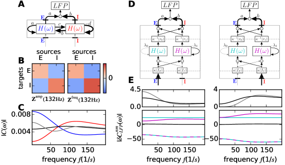
Figure 4: Responses of a symmetric two-dimensional circuit. A Sketch of the circuit. B Sensitivity measure (Eq (22)), showing the anatomical connections shaping the amplitude and frequency of the peak in the spectrum. C Spectra produced by the circuit without input. Red: spectrum of the excitatory population $C_{\mathrm{E}\mathrm{E}}(\omega)$, blue: spectrum of the inhibitory population $C_{\mathrm{I}\mathrm{I}}(\omega)$, gray: LFP $C_{\mathrm{LFP}}(\omega)$ as defined in Eq (25), black: approximation of the LFP by the autocorrelation of the population spectra $C_{\mathrm{LFP}}^{\mathrm{auto}}(\omega)$ as defined in Eq (25). The area under is spectrum between $0\,\mathrm{Hz}$ and $200\,\mathrm{Hz}$ is normalized to one. D Sketches of the eigenmode decomposition of the circuit and the input to the populations. The eigenmodes are characterized by their transfer functions (cyan: mode zero, magenta: mode one). The oscillatory input is applied to either the excitatory (left) or inhibitory (right) population. Gray arrows denote connections with negligible strength. E Upper panel: additional LFP induced by the stimulus. Full signal $\delta C_{\mathrm{LFP}}(\omega)$ (gray curve) and the signal without the crosscorrelation of the input currents $\delta C_{\mathrm{LFP}}^{\mathrm{auto}}(\omega)$ (Eq (27), black curve). Lower panel: decomposition of the excess LFP spectra $\delta C_{\mathrm{LFP}}^{\mathrm{auto}}(\omega)$ into the contribution of the zeroth mode (cyan), the first mode (magenta) and the cross-modes (cyan-magenta). Connectivity parameter: $g=1.4,\>a=1.0,\ b=g,\ c=1.0,\ d=g$.

Symmetric two-dimensional network

A peak in the high $\gamma$-range has been shown to be generated by a network composed of LIF-neuron models with symmetric architecture [31]. In this setup the excitatory and the inhibitory population receive the same input ($a=c=1,\ b=d=g$) (Fig 4A) yielding one eigenvalue to be zero and one to be negative ($\lambda_{0}=0,\ \lambda_{1}=1-g$), for networks working in the inhibition dominated regime ($g>1$). Here the eigenvectors deviate from the vectors of the populations ($\mathbf{e}_{0}$ and $\mathbf{e}_{1}$), revealing that the modes get contributions from both populations. Since the zeroth eigenvalue is zero, the corresponding mode has no feedback (Fig 4D, left) and the produced spectrum, which scales with $1/\left|1-\lambda_{0}H(\omega)\right|$ (Eq (21)), is therefore constant. The first mode generates a peak due to the negative feedback, with a frequency of around $130\,\mathrm{Hz}$ determined by the parameters of its transfer function as well as the strength of the coupling $\lambda_{1}$. The sensitivity analysis shows that this peak is generated by an interplay of the two populations as well as their self-coupling (Fig 4B).

The LFP produced by the circuit without additional input, as well as its decomposition into the spectra observed in the populations, is shown in Fig 4C. Since the population vector of the inhibitory population points more in the direction of the right eigenvector of the first mode than the right eigenvector of the zeroth mode ($\mathbf{u}_{1}^{\mathrm{T}}\mathbf{e}_{1}>\mathbf{u}_{0}^{\mathrm{T}}\mathbf{e}_{1}$), the spectrum of the inhibitory population displays the peak generated by the first mode. The opposite is true for the excitatory population ($\mathbf{u}_{0}^{\mathrm{T}}\mathbf{e}_{0}>\mathbf{u}_{1}^{\mathrm{T}}\mathbf{e}_{0}$) which shows a spectrum dominated by the zeroth mode and the mixture of the zeroth and first mode, which is reminiscent of a low pass filter. Note, however, that this reasoning only holds for modes which are far from an instability. If one of the eigenvalues would approach the value one at a certain frequency, the prefactor in Eq (21) would become large and the corresponding peak would be visible in all populations. However, in the presented regime of weakly synchronized oscillations, the rhythm generated by the full circuit produces similar population rate spectra as the rhythm generated by a single population (compare Fig 4C and Fig 3C). It is notable, that in this circuit the crosscorrelation of the population rate spectra have a large impact on the LFP (Fig 4C ).

Applying a stimulus to one of the two populations elicits large responses originating in the autocorrelations of the modes, as well as in their crosscorrelation (see single color and dashed curves in Fig 4E). The large crosscorrelation can be understood by considering that the same connections contribute to both modes. That was not the case in the previous circuit, where the crosscorrelation therefore remained small. In the current circuit, the sum of the auto- and crosscorrelation is small and thus the resulting spectrum is also small. An example of such a circuit is a network of neurons where the population signal displays small fluctuations, but a projection of the rates onto the direction of the modes yields strongly fluctuating signals, which are highly negatively correlated between the modes.

In quantitative terms, stimulating the excitatory population elicits responses of the modes whose amplitudes scale with $\gamma_{0}=\frac{\sqrt{g^{2}+1}}{g-1}$ and $\gamma_{1}=-\frac{\sqrt{2}}{g-1}$ (Fig 4D, left). The signs of $\gamma_{0}$ and $\gamma_{1}$ reveal that excitation of the two modes is of opposite signs, yielding a negative crosscorrelation (which scales with $\gamma_{1}\gamma_{2}$, see Fig 4E, left). As the population vector of the excitatory population points more in the direction of the right eigenvector corresponding to the zeroth mode than the eigenvector of the first mode ($|\gamma_{0}|>|\gamma_{1}|$), the stimulus induced response visible in the LFP is dominated by contributions of the zeroth mode and the coupling of the zeroth and first mode (Fig 4E left), as already observed in the composition of the spectrum without additional stimulus. Stimulating the inhibitory population also excites both modes ($\gamma_{0}=-\frac{\sqrt{g^{2}+1}}{g-1},\ \gamma_{1}=\frac{g\sqrt{2}}{g-1}$) with opposite signs (Fig 4D, right) such that the main part of the responses cancel. The contribution of the first mode is slightly larger (Fig 4E, right), imposing its peak onto the LFP spectrum.

Thus the responses to stimulations obtained here are similar to the responses of the previously considered circuitry: stimulating the excitatory population elicits mainly slow frequencies, while stimulating the inhibitory population reveals a high frequency peak. These responses can therefore not distinguish between an I-I-loop and a fully connected E-I-circuit generating the high frequency peak.

In principle, it is possible to selectively probe the modes of a complex circuit experimentally. This requires co-stimulation of all populations with population specific stimulus amplitudes chosen proportional to their respective entries in the right-sided eigenvectors $\mathbf{u}_{0}$ and $\mathbf{u}_{1}$.

A two-dimensional network without self-coupling

Recurrently connected excitatory and inhibitory populations can produce oscillations without the necessity of inhibitory self-feedback. The network motif discussed in this section can be considered the prototypical PING motif as discussed in [42], which produces $\gamma$ oscillations.

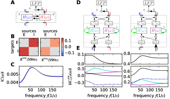
Figure 5: Response to oscillatory input of a two-dimensional circuit without self-coupling. A Sketch of the circuit. B Sensitivity measure (Eq (22)), showing the anatomical connections shaping the amplitude and frequency of the peak in the spectrum. C Spectra produced by the circuit without input. Red: spectrum of the excitatory population $C_{\mathrm{E}\mathrm{E}}(\omega)$, blue: spectrum of the inhibitory population $C_{\mathrm{I}\mathrm{I}}(\omega)$, gray: LFP $C_{\mathrm{LFP}}(\omega)$ as defined in Eq (25), black: approximation of the LFP by the autocorrelation of the population spectra $C_{\mathrm{LFP}}^{\mathrm{auto}}(\omega)$ as defined in Eq (25). The area under is spectrum between $0\,\mathrm{Hz}$ and $200\,\mathrm{Hz}$ is normalized to one. D Sketches of the eigenmode decomposition of the circuit and the input to the populations. The eigenmodes are characterized by their transfer functions (cyan: mode zero, magenta: mode one). Green denotes positive complex values ($\lambda_{0}=i\sqrt{bc}$) and dark green negative complex values ($\lambda_{1}=-i\sqrt{bc}$). The oscillatory input is applied to either the excitatory (left) or inhibitory (right) population. Gray arrows denote connections with negligible or zero strength. E Upper panel: additional LFP induced by the stimulus. Full signal $\delta C_{\mathrm{LFP}}(\omega)$ (gray curve) and the signal without the crosscorrelation of the input currents $\delta C_{\mathrm{LFP}}^{\mathrm{auto}}(\omega)$ (Eq (27), black curve). Lower panel: decomposition of the excess LFP spectra $\delta C_{\mathrm{LFP}}^{\mathrm{auto}}(\omega)$ into the contribution of the zeroth mode (cyan), the first mode (magenta) and the cross-modes (cyan-magenta). Connectivity parameter: $a=0,\ b=0.8,\ c=0.9,\ d=0$.

Fig 5A shows a diagram of a circuit with connections between the populations and negligible self-couplings. In this parameter regime the LFP is determined by the inhibitory activity impinging onto the excitatory neurons. This circuit generates a peak at around $50\,\mathrm{Hz}$, which, as expected, depends on the connections between the populations (Fig 5B). Since the eigenmode producing the oscillations is a mixture of the two populations, with both of them having comparably sized entries in the corresponding eigenvectors, the population spectra are similar in both populations with similar contribution to the LFP (Fig 5C, all curves lie on top of each other). The circuit is characterized by two eigenvalues, which are complex conjugates and purely imaginary ($\lambda_{0,1}=\pm i\sqrt{bc}$). Considering the eigenvalue trajectories (described by $\lambda_{0,1}H(\omega)$) reveals that the trajectory starting at a positive imaginary part produces the $50\,\mathrm{Hz}$ peak, while the other trajectory produces a peak at a very large frequency. The latter one is potentially suppressed in neural circuits by inhomogeneities in the parameters, like distributed delays, which contribute an additional multiplicative factor with low-pass characteristics (cf. Eq (1)) to the transfer function. We hence focus on the peak at lower frequency.

A stimulus applied to either the excitatory or the inhibitory population excites both modes with equal strength ($\gamma_{0}=\gamma_{1}=\frac{1}{2}\sqrt{\frac{bc+1}{bc}}$ for stimulation of the excitatory population and $\gamma_{0}=\gamma_{1}^{*}=\frac{i}{2}\sqrt{bc+1}$ for stimulation of the inhibitory population, illustrated in Fig 5D). Since $\gamma_{0}\gamma_{1}^{*}>0$ when stimulating the excitatory and $\gamma_{0}\gamma_{1}^{*}<0$ when stimulating the inhibitory population, the contribution of the crosscorrelations to the response spectrum is of opposite sign for the two stimuli, as seen in Fig 5E (dashed curves). The cancellations of the cross- and autocorrelation when stimulating the excitatory population yields an LFP response, which is reminiscent of a low-pass filter with a small peak at very low frequencies (Fig 5E, left upper panel). Since no cancellation occurs when stimulating the inhibitory population, the spectrum shows amplifications at the frequency that is generated by the circuit autonomously (Fig 5E, right upper panel). Hence, also with this circuit motif, stimulation of the inhibitory population yields a peak in the LFP which is missing when stimulating the excitatory population, even though the excitatory population is involved in generating the peak.

In order to isolate the response of one mode, the stimulus vector needs to point in the direction of its right eigenvector. Since the eigenvectors are complex, with real entries for the excitatory and imaginary entries for the inhibitory population ($\mathbf{u}_{0,1}=\sqrt{\frac{1}{bc+1}}\left(\sqrt{bc},e^{\mp i\pi/2}\right)$), adjusting the amplitude of the sinusoidal signal applied to the population is not sufficient to segregate the mode responses. Since the Fourier transform of a phase-shifted sine wave is given by $\mathcal{F}[sin(\omega_{0}t+\phi)]=e^{i\omega/\omega_{0}\phi}\mathcal{F}[\sin(\omega_{0}t)]$, complex entries in the stimulus vector can be achieved by adjusting the relative phase of the input to the populations. The mode generating the peak around $50\,\mathrm{Hz}$ is excited in isolation if the stimulus applied to the inhibitory population lags the stimulus to the excitatory population by $\pi/2$. Reversely, if the excitation of the inhibitory population precedes the stimulation of the excitatory population by $\pi/2$, the LFP response is determined by the first mode, which amplifies fast oscillations.

Stimulus evoked spectra in a model of a microcircuit

In this section we analyze the responses observed in a model of a microcircuit of the primary sensory cortex to oscillatory input, discuss the results in comparison with experimental data and point out potential pitfalls when utilizing these results to identify the anatomical sources of oscillations produced by the circuit. First, a previously introduced theoretical framework, which enables the prediction of population rate spectra as well as the location of their origin, is extended by oscillatory input. Subsequently we demonstrate that the theoretical prediction reproduces the responses observed in simulations and additionally offers insight into the anatomical origin of the components contributing to these responses. Analyzing the responses of the populations in layer 2/3, we demonstrate that ad-hoc interpretations can yield misleading conclusions.

The microcircuit with oscillatory input

The microcircuit model has been introduced by Potjans et al. [36] to represent a layered circuit typical for the primary sensory cortex. The model is composed of around $10^{5}$ LIF model neurons, which are divided into four layers (L2/3, L4, L5, L6) with one excitatory and one inhibitory population each. Connection probabilities between theses eight populations are gathered from 50 anatomical and physiological studies. The model has been shown to reproduce typical rate profiles [36]. In agreement with experimental evidence it supports the emergence of slow rate fluctuations in layer 5, as well as low- and high-$\gamma$ oscillations in the upper layers [34]. As yet, the microcircuit has only been analyzed in the resting state, when each population receives uncorrelated Poisson input, which mimics the input of remote areas. Oscillatory stimuli are introduced by modulating a ratio $a$ ($0<a<1$) of the external input rate to the populations with a sinusoid of a given frequency $f_{\mathrm{ext}}$

$$\nu_{\mathrm{ext}}^{k}(t)=\nu_{\mathrm{ext}}^{0}N_{\mathrm{ext}}^{k}(1+a\,\sin(2\pi f_{\mathrm{\mathrm{ext}}}t)).$$ (28)

Here $\nu_{\mathrm{ext}}^{k}(t)$ denotes the total external input applied to the $k$-th population, $\nu_{\mathrm{ext}}^{0}$ the firing rate associated with one incoming connection and $N_{\mathrm{ext}}^{k}$ the external indegree to population $k$.

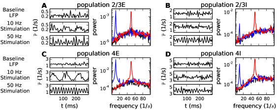
Figure 6: Population rate responses to oscillatory stimuli. A Left: Instantaneous firing rate of population 2/3E of the microcircuit in the resting state (top) and with additional sinusoidal stimulus (Eq (28)) of frequency $10\,\mathrm{Hz}$ (middle) and $50\,\mathrm{Hz}$ (bottom) applied to population 2/3E. Right: Corresponding power spectra of the rates in population 2/3E in the resting state (black) and with additional stimuli ($10\,\mathrm{Hz}$: blue, $50\,\mathrm{Hz}$: red). B-D Instantaneous firing rates and power spectra of populations 2/3I, 4E, and 4I as in A, with the stimuli applied to the respective population.

Fig 6 shows the instantaneous firing rate, as well as the spectra observed in populations 2/3E, 2/3I, 4E, and 4I in the resting state and with oscillatory input of $10\,\mathrm{Hz}$ and $50\,\mathrm{Hz}$ to the populations of strength $a=0.05$. The spectra show that this modulation of $5$ percent of the external static input suffices to reproduce population responses of strength comparable to LFP responses measured in experiments applying oscillatory light stimuli to optogenetically altered mice (see Fig. 3c in [10]). The rate of population 4E adapts strongly to both rhythms (see left panel of Fig 6C), which is interesting since layer 4 is considered the main recipient of thalamic input [36]. In the microcircuit, excitatory populations show a stronger amplification of the $10\,\mathrm{Hz}$ stimulus, while the inhibitory populations show higher amplitudes when stimulated with $50\,\mathrm{Hz}$ (Fig 6). These results agree with measurements conducted by Cardin et al. (Supplementary Fig. 5 in [10]) by trend: Low frequency stimulation of excitatory neurons show stronger responses in the LFP than stimulation of inhibitory neurons and vice versa for high frequency stimulations. However, both excitatory and inhibitory currents contribute to the LFP [41], such that the measured responses in experiments should be compared with a superposition of the individual population rate spectra.

The effect that low frequency stimulation of excitatory populations evokes strong responses can be understood intuitively: Our previous examples show that excitatory populations more prominently participate in modes that resemble low-pass filters. In other words, excitatory activity and, in particular, excitatory self-feedback drive the circuit towards a rate instability which facilitates slowly decaying modes. Responses of these modes are also elicited when stimulating the excitatory population at low frequencies, resulting in amplified low frequency responses.

Theoretical description of oscillatory input

Here we describe how the amplification of oscillatory stimuli can be understood theoretically. Previous work [34] shows that the population rate spectra produced by this model are sufficiently described by a theoretical two-step reduction composed of mean-field theory, which yields the stationary firing rates [43, 30], as well as linear response theory, which characterizes the response properties of the neurons [31, 32, 33], formally described by the dynamic transfer function. Since already small modulations of the external input have considerable impact on the population rate spectra, but negligible effect on the stationary firing rates (Fig 6), we constrain our analysis in this section to purely oscillatory stimuli which do not alter the working point of the populations. This assumption can be justified by the observation that the width of the response peaks shown in Fig 6 is narrow (in particular for high frequencies) and the stimulated frequency therefore approximately does not couple to other frequencies. The network can therefore be analyzed analogously to the two-dimensional circuits discussed in the previous section, after mapping the dynamics in the microcircuit model to interacting linear rate models [34]. Extensions to stimuli that affect the stationary state of the system are discussed in “Approximation of the dynamic transfer function”. The spectrum as well as the excess spectrum $\delta\mathbf{C}(\omega)$ of the microcircuit with sinusoidal input are hence described by the same equation as the 2d-circuit (Eq (21), Eq (26)) extended to eight populations (for detail see “Composition of the spectrum with input”)

$$\delta\mathbf{C}(\omega)=\mathbf{C}_{I}(\omega)-\mathbf{C}(\omega) =\sum_{n,m=1}^{8}\frac{\beta_{\mathrm{ext},nm}(\omega)}{(1-\lambda_{n}(\omega))(1-\lambda_{m}^{*}(\omega))}\mathbf{u}_{n}(\omega)\mathbf{u}_{m}^{\mathrm{T}*}(\omega),$$ (29)

with (Eq (76))

$$\beta_{\mathrm{ext},nm}(\omega)=w_{\mathrm{ext}}^{2}N_{\mathrm{ext},k}^{2}\nu_{\mathrm{ext}}^{2}a^{2}\frac{T}{4}\left|H_{k}(\omega_{\mathrm{I}})\right|^{2}\alpha_{n}^{k}(\omega)\alpha_{m}^{k*}(\omega).$$ (30)

The latter factor, which quantifies the amplitude of the excited auto and cross-correlations of the modes, depends on the modulated external firing rates $N_{\mathrm{ext},k}\nu_{\mathrm{ext}}a$, the external synaptic weights $w_{\mathrm{ext}}$, the transfer function of the population that receives the input $H_{k}(\omega_{\mathrm{I}})$, the projection of the modes on the direction of the stimulus $\alpha_{n}^{k}(\omega)=\mathbf{v}_{n}^{\mathrm{T}}(\omega)\mathbf{e}_{k}$ as well as the measurement time $T$.

Since the populations are set at different working points, which is reflected in different population specific firing rates and transfer functions, the left and right eigenvectors are frequency dependent, in contrast to the models considered in the previous sections. The power ratio, which describes the relative size of the evoked spectrum at stimulation frequency, is given by

$$\rho(\omega)=\frac{\mathbf{C}_{I}(\omega)}{\mathbf{C}(\omega)}=1+\frac{\delta\mathbf{C}(\omega)}{\mathbf{C}(\omega)}$$ (31)

and evaluated at stimulus frequency $\omega=\omega_{I}$. To show that the theoretical description suffices to predict the impact of oscillatory input to the population rate spectra, we modulate $5\,$percent of the static external input to each population at frequencies between $0$ and $200\,\mathrm{Hz}$ and compare the power ratios at stimulation frequency observed in each population with the theoretically predicted power ratios (Fig 7). As expected, the response to a stimulus is strongest in the population the stimulus is applied to (see the diagonal panels in Fig 7).

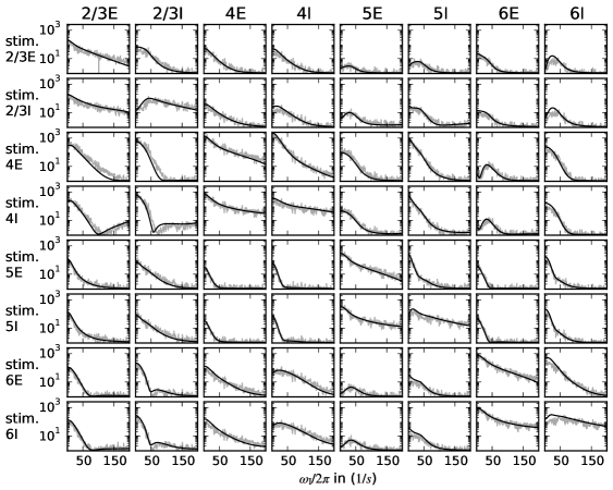
Figure 7: Power ratios of population rate spectra with oscillatory stimuli. Each column shows the power ratios (Eq (31)) of one population (gray: simulation, black: theoretical prediction). The rows indicate the population the stimulus is applied to. The stimulus is applied as a sinusoidal modulation of $5$ percent of the external static input rate and oscillates with frequencies between $0$ and $200\,\mathrm{Hz}$ in steps of $1\,\mathrm{Hz}$. The power ratio is measured at the frequency of the stimulus.

Considering only the diagonal panels, it is evident that stimuli applied to excitatory populations amplify mostly low frequencies, which confirms the previously found tendencies. The inhibitory populations, except for 4I, display resonances at frequencies larger than zero. The most prominent peak is visible in population 2/3I, which, due to its location at just above $40\,\mathrm{Hz}$, could be interpreted as a resonance phenomenon related to the low-$\gamma$ peak produced by the circuit. The responses of 2/3E and 2/3I (Fig 8A0, B0) show similar tendencies as the LFP power ratio measured in experiments (see Fig. 3 in [10]), namely 2/3E supports mainly low frequencies, while 2/3I displays a resonance at around $41\,\mathrm{Hz}$. However, it remains to be investigated whether the peaks in the population rate spectra would also be visible in the LFP, which is given as a weighted sum of the spectra of one row in Fig 7 in addition to the crosscorrelations of the currents (as outlined for an examplary 2d-circuit in “Approximation of the LFP”).

The origin of the peak visible in the population rate spectrum of 2/3I

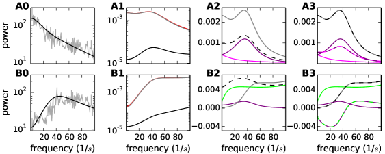
Figure 8: Composition of power ratio in populations 2/3E and 2/3I. A0 Power ratio of population 2/3E with oscillatory input to 2/3E (gray: simulation, black: theoretical prediction, see Fig 7). A1 Population rate spectrum of population 2/3E in the resting state (black, $\mathbf{C}_{0}(\omega)$) and with oscillatory input (red, $\mathbf{C}_{\mathrm{I}}(\omega)$, Eq (77)). The gray curve indicates the additional power induced by the stimulus (excess spectrum: $\mathbf{C}_{\mathrm{I}}(\omega)-\mathbf{C}_{0}(\omega)$). A2 Contributions due to the autocorrelation of the modes (see Eq (29) for $n=m$, colored curves) to the excess spectrum (gray curve). Different colors correspond to different modes, with their anatomical origin shown in Fig 9. Only the dominant contributions are shown. Each mode can be attributed to the generation of (at most) one peak (for the modes shaping the oscillations in the microcircuit see Methods in [34] and Fig 9). The sum of all contributions originating in the autocorrelations of the modes is depicted by the black dashed curve. A3 As in A2 including the contribution originating in the crosscorrelation of the modes (see Eq (29) for $n\neq m$). The identities of the modes contributing to the pairwise contributions are reflected in the color-composition of the curves. The sum of all contributions (black dashed curve) is identical to the entire excess spectrum (gray curve). B0-B3 Same as in A0-A3, for the population rate dynamics observed in population 2/3I with oscillatory input to population 2/3I. The areas underneath the curves of the sum of all modes deviate from the area underneath the curve of the sum of the two shown modes by 4% (A2), 7% (B2), 21% (A3) and 20% (B3).

In the following, the results of the last sections are exploited to analyze whether and how the peak in the power ratio of population 2/3I can shed light on the circuit producing the low-$\gamma$ oscillation. Since power ratios can give misleading results, especially if the resting spectra are not entirely flat (as discussed in “Dynamic responses of a self-coupled inhibitory population”), the resting state spectra as well as the response and excess spectra are shown in Fig 8A1 and Fig 8B1. The response spectra are between one to two orders of magnitude larger than the resting state spectra and are therefore approximately equivalent to the excess spectra. The excess spectrum for population 2/3E shows a peak in the low-$\gamma$ frequency range, as well as a large offset for low frequencies. Since the stimulus amplifies low frequencies stronger than the low-$\gamma$ peak, the $\gamma$ peak is not visible in the power ratio. The excess spectrum visible in 2/3I has a contrary tendency: it is weak for low frequencies and saturates at a higher value for frequencies above $40\,\mathrm{Hz}$. The peak in the power ratios originates in the prompt increase of the excess spectrum between $20$ and $40\,\mathrm{Hz}$.

In the following we decompose the excess spectrum into contributions from the respective dynamic modes (see “Theoretical description of oscillatory input”) and identify the dominant contributions at peak frequency $41\,\mathrm{Hz}$. Subsequently we employ the recently derived sensitivity measure [34] to trace the dominant modes back to their anatomical origin.

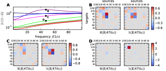
Figure 9: Anatomical origins of the modes contributing to the response spectra. A Frequency dependence of the factors $\left|1/(1-\lambda_{i}(\omega))\right|$ that shape the population rate spectra. Each of the eight factors is associated with a sub-set of connections, which varies with frequency. The dominant contributions to the responses of population 2/3E and 2/3I are given by the modes whose eigenvalues are associated to the purple, pink, and green curves. The peak frequency is marked by solid black dots, alongside with a letter denoting the panel that shows the associated connections. B Real and imaginary part of the sensitivity measure (Eq (23)) evaluated at $47\,\mathrm{Hz}$. Strong colors reflect connections which are strongly present in the corresponding mode. C, D Anatomical origin of pink and green curves, as in B.

We recall from the previous chapters, that the spectrum visible in one population is composed of contributions arising from the autocorrelation as well as the crosscorrelation of the modes. If the peak in the power ratio of population 2/3I would reflect the resonance of one sub-circuit, one would expect the excess spectrum to be composed mainly of the contribution of the corresponding mode. The diagonal contributions to the excess spectrum are given by

$$\delta\mathbf{C}_{\mathrm{auto}}(\omega)=\sum_{n=1}^{8}\frac{\beta_{\mathrm{ext},nn}(\omega)}{\left|1-\lambda_{n}(\omega)\right|^{2}}\,\mathbf{u}_{n}(\omega)\mathbf{u}_{n}^{T*}(\omega).$$ (32)

The dominant contributions originating in the autocorrelations of the modes as well as the sum of all contributions, are shown in Fig 8A2 and Fig 8B2. The main contribution to the low-$\gamma$ peak in the excess spectrum of population 2/3E is indeed given by the trajectory corresponding to the origin of the low-$\gamma$ peak (compare dashed to purple curve), which is determined by connections located in layer 2/3 and 4 (Fig 9B). The eigenvalue trajectory, that gives rise to the low-$\gamma$ peak, originates in a pair of complex conjugate eigenvalues (see Fig 9A at frequency zero, where their absolute values agree), similar to the eigenvalues in the exemplary circuit where the rhythm was entirely determined by the coupling between the excitatory and the inhibitory population rather than their self-coupling (see “A two-dimensional network without self-coupling”). Hence the modes corresponding to the complex conjugated pair of eigenvalues are shaped by the same connections and a stimulus applied to population 2/3E also elicits a response of the mode associated to the counterpart of the low-$\gamma$ eigenvalue (see pink trajectory, its origin Fig 9C and its contribution to the excess spectrum Fig 8A2). However, even though the peak shape appears to be formed by these modes, the offset of the excess spectrum cannot be explained by the diagonal contributions alone (compare dashed to gray curve). Population 2/3I contributes to the generation of two different peaks, the low-$\gamma$ oscillation, as well as a high-frequency oscillation originating in the self-coupled population alone (see green eigenvalue trajectory in Fig 9A and its origin in Fig 9D). Hence, stimulating population 2/3I elicits responses of modes with different anatomical origins (Fig 8B2). The sum of contributions originating in the autocorrelations, however, deviates considerably from the total excess spectrum. This shows that crosscorrelations between the modes play a role.

The total excess spectrum can be reproduced by adding the largest terms of the cross-contributions between the modes, which are given by

$$\delta\mathbf{C}^{\mathrm{cross}}(\omega)=\sum_{n,m=1,m<n}^{8}\Re\left(\frac{\beta_{\mathrm{ext},nm}(\omega)}{(1-\lambda_{n}(\omega))(1-\lambda_{m}^{*}(\omega))}\,\mathbf{u}_{n}(\omega)\mathbf{u}_{m}^{T*}(\omega)\right).$$ (33)

The contributions to the spectrum due to the crosscorrelations between the dominant modes are shown in Fig 8A3 and Fig 8B3. For population 2/3E the crosscorrelation between the two modes is positive and provides the missing offset to the excess spectrum. For population 2/3I, the crosscorrelation between the mode associated to the low-$\gamma$ peak and the self-coupling of population 2/3I is negative below $40\,\mathrm{Hz}$.

In other words, providing oscillatory input between $0\,\mathrm{Hz}$ and $40\,\mathrm{Hz}$ to population 2/3I elicits large responses of two modes. The responses of the modes are given by weighted linear combinations of the population rates corresponding to a multiplication of the rate vector containing all rates with the left eigenvector of the modes. However, the anti-correlation between the modes at low frequencies, which is strongest at $20\,\mathrm{Hz}$, lowers the fluctuations in the total response of population 2/3I. Since the amplitude of the negative correlation decreases for larger frequencies, a peak appears in the power ratios. This peak could be misinterpreted as the self-coupling of population 2/3I to generate an oscillation in the low-$\gamma$ frequency range, even though the peak is generated by a more complex sub-circuit in the upper layers.

Discussion

In this manuscript we analyze the responses of networks, that generate oscillations internally by means of embedded sub-circuits, to oscillatory stimuli and demonstrate how the stimulus is reflected in different measures of the network response. We first employ a sequence of phenomenological rate models, each of which illustrating one dynamical effect that crucially shapes the response. Finally, we apply these insight to circuits composed of populations of LIF model neurons that can be mapped to the former class of models analytically. Our results shed light on the amount of information regarding the anatomical origin of produced oscillations that can be inferred from the responses to oscillatory stimuli. The insights outlined here can be exploited to design stimulation protocols that uncover dynamically relevant sub-circuits.

Theoretical advances have been made to explain the results of Cardin et al. [10], who have shown that inhibitory neurons exhibit a resonance in the $\gamma$ frequency regime when stimulated with oscillatory light pulses, while excitatory neurons amplify low frequencies. Theoretical studies reproduced these results by considering certain neuronal or synaptic dynamics. Tchumatchenko et al. [22] assume sub-threshold resonances of inhibitory neurons as well as gap junctions between them and Tiesinga [23] considers slow synaptic currents for the connections from the excitatory to the inhibitory neurons. Here we investigate the effect of the network architecture on the measured responses. Using three characteristic connectivity motifs of an E-I-circuit, we identify connectivity motifs that yield responses resembling those shown in Cardin et al. We also demonstrate how these results crucially depend on the size of the stimulus as well as on the measure of the network response.

The effect of small versus large stimulus amplitudes

The effect of stimuli on the dynamics of a circuit can be classified into three regimes. In the simplest case, additional input can be treated as a small perturbation, which does not influence the dynamical state of the circuit (as done in [22]). In this case, the stimulus can be treated analogously to the internally generated noise of the population rates, which is, for example, produced within networks of LIF neurons of finite size [32, 44, 45, 46, 47, 48, 49]. In this setting, external input to populations of LIF neurons can be described as a modulation of the synaptic input, which is filtered by the dynamic transfer function of the populations the stimulus is applied to. The dynamic transfer function is typically a low-pass filter yielding the emphasis of low frequencies by the network response. This explanation is similar to the results in [27], where the externally applied signal is described by an Ornstein-Uhlenbeck process and the low-pass filter is therefore explicitly introduced. Since the elevated low-frequency components in the network response contain the filter properties of individual populations rather than network dynamics, we suggest a modified stimulation protocol which eliminates the effect of the initial filtering and therefore enables the analysis of a signal which emerges from internal network dynamics alone.

An input that affects the stationary properties of the circuit may change the working point within the linear regime of the static transfer function. The dynamical properties of the circuit then stay approximately unaltered and only the change of the stationary rates needs to be accounted for. In contrast, an input that changes the stationary rates in the nonlinear regime also changes the dynamic transfer functions of the populations, which potentially alters the dynamic behavior of the entire network. We show that this change can often be approximated by adjusting the prefactor of the dynamic transfer function (see “Approximation of the dynamic transfer function”). Applying this approximation to describe constant positive input to a self-coupled inhibitory population, which generates a distinct frequency, shows that the peak in the spectrum increases, while its peak frequency remains unaltered. In other words, the eigenvalue trajectory which determines the dynamics of the circuit is shifted towards instability by the constant input, while its shape remains unaltered. Since this effect dominates the response spectrum compared to changes evoked by a purely oscillatory stimulus, this finding supports the statement by Tiesinga et al. [24], who suggested to employ constant stimuli as an alternative to oscillatory stimuli to investigate the origin of oscillations experimentally. The result is in line with the high sensitivity of the low-$\gamma$ power to the external input to population 4E: the microcircuit model used in this paper is derived from the model employed in [34] by reducing the external input to population 4E and shows strongly reduced oscillations in the low-$\gamma$ range.

The approximation of the modified dynamic transfer function by a change in the prefactor needs to be applied with caution, when the population is embedded in a network. Here the static transfer function can show higher degrees of nonlinearity due to the recurrent feedback. As a result a stimulus is more likely to change the dynamic structure of the network. These effects can only be captured by linearizing the system around the new working point. An analytical description of the transition between the resting state and the stimulus induced state remains to be investigated. Recent results on the nonlinear transfer function of the LIF model will be useful in this approach [50].

In summary, the results derived here show that the way in which a stimulus affects the dynamical regime of a network, as well as the filtering properties of the populations, should be taken into account when probing a network for the origin of internally generated oscillations.

Power ratios versus response spectra

Experimental studies [10] demonstrate the responses to oscillatory stimuli by means of power ratios, the LFP power at stimulus frequency normalized by the LFP power at that frequency at rest. Theoretical studies, on the contrary, consider normalized network responses [22] as well as absolute responses at stimulus frequency [23].

We analyze the effectiveness of detecting the anatomical origin of oscillations when using power ratios compared to response spectra evoked by oscillatory stimuli. Power ratios can yield misleading results if the spectrum at rest is not entirely flat. In these cases it appears advantageous to consider the difference of the spectra with and without additional stimulus. Small stimuli that do not affect the stationary dynamics of the circuit evoke responses of oscillatory modes that are also responsible for the oscillations in the resting condition. The peaks may be canceled in the relative spectrum and therefore information can get lost when considering power ratios. In particular, in one-population systems the power ratio becomes independent of the intrinsic resonance phenomena of the network and reflects the filter properties of the population. In higher dimensional systems, a stimulation protocol which allows for the reconstruction of all circuit internal variables (Eq (77)) can, in principle, be designed from the population rate spectra and cross-spectra obtained by separately stimulating each population. Applications of stimuli that affect the stationary dynamics of the circuit in the nonlinear regime, however, change the dynamic response properties of the circuit. If the response properties are changed such that the resonance of an oscillatory mode is strengthened, these effects can dominate and also show up in power ratios. Therefore, we propose to consider both, absolute and relative spectra.

Connecting network responses to dynamic network architecture

Oscillations induced by the network structure can either be generated by the self-coupling of one population and imposed onto other populations or by the interplay of several populations. We analyze here whether the involvement of one population in the generation of an oscillation can be investigated by means of oscillatory stimuli to that population. We show how the network response to oscillatory stimuli can be decomposed into responses generated by the auto- as well as crosscorrelation of dynamic modes. Each mode can, individually, be traced back to its anatomical origin, namely the sub-circuit that generates the associated oscillation. However, in the analysis of experimental or simulated data, such decomposition into modes is inaccessible. The anatomical origin of the oscillation could therefore only be inferred from responses generated by a single mode. It turns out that the stimulation of an individual population elicits the response of a single mode only in trivially connected circuits, in which the connections between populations are negligible. In more complicated circuits, populations typically participate in multiple dynamical modes, which are activated together when stimulating that population.

The mode composition of the network response depends on the considered measure of the network response. Experiments typically measure LFP responses [10], which have been linked to the input onto excitatory neurons [40, 41]. Tchumachenko et al. [22] defined the network response as the response of the population that is stimulated and therefore measured different responses depending on the stimulus. Tiesinga [23] considers the activity of the excitatory cells. These two theoretical studies referred to the findings presented by Cardin et al. who showed that that the $\gamma$-resonance was present in the LFP ratio when stimulating the inhibitory cells at $\gamma$ frequency, but was missing when stimulating the excitatory cells. Given that the connectivity plays a role in the composition of the LFP, it is possible that a resonance is visible in the population spectrum, but not in the LFP response (see for example the spectra of the two-dimensional network without self-coupling Fig 5B). In the presented example, the feedback of the excitatory population response is missing and the $\gamma$ rhythm is therefore not relayed back to the pyramidal neurons where it would contribute to the LFP. Even though an E-I network with a missing E-E-loop might not be biologically realistic, the same effect could be caused by a large amount of NMDA receptors at the synapses of the excitatory neurons: The slow synapses then act as a low-pass filter which the $\gamma$ oscillation cannot pass (the same mechanism was investigated in [23]). In other words, the connection would not be present dynamically at $\gamma$ frequency.

To test the hypothesis that the findings of Cardin et al. suggest an oscillation generating mechanism which solely involves the inhibitory neurons, we compare the responses of two exemplary circuits (see “A self-coupled inhibitory circuit embedded in a two-dimensional network” and “Symmetric two-dimensional network”). In the first circuit, the $\gamma$ oscillation is generated by the I-I-loop and subsequently imposed onto the excitatory population. The second circuit, in contrast, requires all connections for the generation of $\gamma$. We show that the LFP response to oscillatory stimulation of the inhibitory neurons shows a resonance at $\gamma$, while the response to stimulated excitatory neurons resembles a low pass filter, regardless of the origin of the oscillation. We therefore conclude, similarly to [24], that oscillatory stimuli cannot exclude the involvement of excitatory neurons in the oscillation generating mechanism.

We discuss the design of a stimulation protocol that isolates the responses of individual dynamic modes by exciting populations in the same ratio in which they contribute to the oscillation generating sub-circuit. However, it remains an open question how these single mode responses can be distinguished from mixtures of mode responses without the knowledge of the dynamic transfer of the mode. It is also debatable whether this protocol is experimentally feasible, given that, if the structure of the mode were unknown, numerous runs in which several populations are stimulated with various strength and time lags would be required.

The emergence of ambiguous resonances in the network response of a microcircuit model

Applying oscillatory stimuli to the populations in a multi-layered model of a column composed of LIF model neurons demonstrates that the response spectra in large spiking networks can be predicted theoretically. The results (Fig 7) show that stimuli evoking firing rate fluctuations as large as the firing rate itself (see left panel in Fig 6C) as well as response spectra of amplitudes comparable to those evoked in experiments [10] (see right panels in Fig 6), can still be sufficiently well described by the employed theoretical framework, which is based on mean-field and linear response theory.

The power ratios of population rates with oscillatory stimuli applied to the respective population reveal a resonance in the low-$\gamma$ frequency range when stimulating population 2/3I. However, it has been shown that the low-$\gamma$ peak is generated within a sub-circuit which is located in the upper layers and involves several populations [34]. Decomposing the network response at $\gamma$ frequency into contributions of the dynamic modes that shape the oscillations in the microcircuit model, reveals that the response is mainly shaped by two modes including their crosscorrelation; in addition to the mode that is responsible for the low-$\gamma$ peak, population 2/3I contributs strongly to the mode which is composed of the 2/3I-2/3I loop and which is responsible for the generation of a peak at very high frequencies [34]. Stimulating population 2/3I therefore elicits responses of both modes, which are anti-correlated for low frequencies and therefore cancel the contributions of the autocorrelations of the modes. This cancellation for low frequencies, but not for high frequencies, gives rise to a peak in the power ratio that could be misinterpreted as the signature of an underlying I-I loop that generates the low-$\gamma$ peak.

In summary, we demonstrate the importance of correctly identifying the dynamic influence of the stimulus on the system as well as the considered output measure when interpreting experimental results. By analyzing reduced circuits as well as a model of a column in the primary sensory area, we demonstrate that the entire underlying network needs to be taken into account when interpreting emerging signals with respect to the origin of oscillations.

Methods

Static and dynamic transfer function of LIF-neurons

The description of the population dynamics discussed here follows the outline in [51] and the terminology has been introduced in [26]. Activity entering one population can be regarded as first passing a linear filter $g(t)$ (dynamic transfer function) and subsequently being sent through a static nonlinear function (static transfer function) (see Fig. 1B in [51]). Hence the rate of one population of unconnected neurons receiving white noise input $x(t)$ with strength $I_{0}$ can be described as

$$r(t)=\nu([g\ast I_{0}x](t))\approx r_{0}+I_{0}\nu^{\prime}(0)\,[g\ast x](t),$$ (34)

where $\ast$ denotes the convolution of two signals. In the second step, the nonlinear function was linearized around the static point (also referred to as the working point) with $\nu(0)=r_{0}$. The linearized version of the linear-nonlinear model above can be mapped to the dynamics of LIF neuron models. Here, we consider LIF model neurons with exponentially decaying synaptic currents, i.e. with synaptic filtering. The dynamics of the membrane potential $V$ and synaptic current $I_{\mathrm{s}}$ are given by [30]

$$\tau_{m}\frac{dV}{dt} = -V+I_{s}(t)$$

$$\tau_{\mathrm{syn}}\frac{dI_{s}}{dt} = -I_{s}+\tau_{m}\sum_{j=1}^{N}J_{j}\,s_{j}(t-d_{j})\,,$$ (35)

where $\tau_{m}$ is the membrane time constant and $\tau_{\mathrm{syn}}$ the synaptic time constant. The membrane resistance $\tau_{m}/C_{\mathrm{m}}$ has been absorbed into the definition of the current. Input is provided by the presynaptic spike trains $s_{j}(t)=\sum_{k}\delta(t-t_{k}^{j})$, where the $t_{k}^{j}$ mark the time points at which neuron $j$ emits an action potential. The synaptic efficacy is denoted as $J_{j}=\tau_{\mathrm{syn}}w_{j}/C_{m}$, with $w$ in Ampere. Whenever the membrane potential $V$ crosses the threshold $V_{\theta},$ the neuron emits a spike and $V$ is reset to the potential $V_{\mathrm{r}}$, where it is clamped during $\tau_{r}$. In the diffusion approximation the dynamics reads [30]

$$\tau_{m}\frac{dV}{dt} = -V+I_{\mathrm{s}}(t)$$

$$\tau_{\mathrm{syn}}\frac{dI_{\mathrm{s}}}{dt} = -I_{\mathrm{s}}+\mu+\sigma\sqrt{\tau_{m}}\,\xi(t),$$ (36)

where the input to the neuron is characterized by its mean $\mu$ and a variance proportional to $\sigma$, and $\xi$ is a centered Gaussian white process satisfying $\langle\xi(t)\rangle=0$ and $\langle\xi(t)\xi(t^{\prime})\rangle=\delta(t-t^{\prime})$. The static transfer function $\nu$ can be obtained for white noise (originating from $\delta$-synapses, i.e. $\tau_{\mathrm{syn}}=0$) [28] or colored noise (originating from filtered synapses, i.e. $\tau_{\mathrm{syn}}\neq 0$) [30]. The stationary rate is then given by $r_{0}=\nu(\mu,\sigma)$. The dynamic transfer function $h(t)=\nu^{\prime}(0)g(t)$ has been derived in the Fourier domain using linear response theory to systems exposed to white [32] and colored noise [33]. To employ linear response theory, the system has to be linearized around the static point, yielding a dynamic transfer function that also depends on the working point $H(\omega):=H(\omega,\mu,\sigma)$. The dynamic transfer function of the LIF model with $\delta$-synapses is given by [32]

$$H_{\mathrm{WN}}(\omega,\mu,\sigma)=G\,\frac{1}{1+i\omega\tau_{m}}\frac{\Phi_{\omega}^{\prime}|_{x_{\theta}}^{x_{R}}}{\Phi_{\omega}|_{x_{\theta}}^{x_{R}}},$$ (37)

where $G=\frac{\sqrt{2}r_{0}}{\sigma}$ and we introduced $\Phi_{\omega}(x)=u^{-1}(x)\,U(i\omega\tau-\frac{1}{2},x)$ as well as $\Phi_{\omega}^{\prime}=\partial_{x}\Phi_{\omega}$. Here, $U(i\omega\tau-\frac{1}{2},x)$ is the parabolic cylinder function [52, 5] and the boundaries are $x_{\{R,\theta\}}=\sqrt{2}\,\frac{\{V_{R},V_{\theta}\}-\mu}{\sigma}$. The effect of the synaptic filtering $\sim\tau_{\mathrm{syn}}$ is twofold: First, input is low-pass filtered by the factor $\frac{1}{1+i\omega\tau_{\mathrm{syn}}}$ appearing in the transfer function. Second, it causes a shift of the boundaries [33], i.e. $x_{\{\tilde{R},\tilde{\theta}\}}=\sqrt{2}\frac{\{V_{R},V_{\theta}\}-\mu}{\sigma}+\sqrt{\frac{\tau_{\mathrm{syn}}}{2\tau_{m}}}$, which is correct up to linear order in $k=\sqrt{\frac{\tau_{\mathrm{syn}}}{\tau_{m}}}$ and valid up to moderate frequencies. Finally the dynamical transfer function is given by

$$H(\omega,\mu,\sigma)=G\,\frac{1}{1+i\omega\tau_{m}}\frac{1}{1+i\omega\tau_{\mathrm{syn}}}\frac{\Phi_{\omega}^{\prime}|_{x_{\tilde{\theta}}}^{x_{\tilde{R}}}}{\Phi_{\omega}|_{x_{\tilde{\theta}}}^{x_{\tilde{R}}}}.$$ (38)

Note that we only consider the dominant part of the dynamical transfer function, i.e. the modulation of the output rate caused by a modulation of the mean input. The part of the transfer function corresponding to a modulation of the variance of the neurons’ input [5, 33] is one order of magnitude smaller and neglected here. The formalism for rate fluctuations of a single unconnected population can be extended to an $N$-dimensional recurrent network of populations with the connectivity matrix $\mathbf{M}^{A}$ and delays $d$, where each population receives input from other populations, each of which described as a rate $r_{i}(t)$ with additional noise $x_{i}(t)$ which is subsequently filtered by the population specific dynamic transfer function $h_{i}(t)$

$$r_{i}(t)=h_{i}\ast\sum_{j=1}^{N}M_{ij}^{A}\left(r_{j}(\circ-d_{ij})+x_{j}(\circ-d_{ij})\right).$$ (39)

Here, $h$ is obtained from the Fourier transform of $H$. The connectivity matrix $\mathbf{M}^{A}$ follows from the LIF-network parameters, i.e. $M_{ij}^{\mathrm{A}}\equiv\tau_{m}I_{ij}J_{ij}$, with $I_{ij}$ being the indegree from population $j$ on population $i$.

Approximation of the dynamic transfer function

The dynamical response to a constant current, in the following termed the DC limit, can be obtained by evaluating the dynamic transfer function at frequency zero, i.e.

$$A(\mu,\sigma):=H(0,\mu,\sigma) = \frac{\partial\nu(\mu,\sigma)}{\partial\mu}\,.$$ (40)

The equal sign follows from the fact that the integral over the impulse response $h(t)=\mathfrak{F}^{-1}[H(\omega)](t)$ is given by the response to a constant input [53]. We now investigate how the dynamic transfer function behaves for an isolated population which receives external input defined by its mean $\mu$ and variance $\propto\sigma^{2}$

$$\mu =\tau_{m}K_{\mathrm{ext}}J_{\mathrm{ext}}\nu_{ext},\qquad\sigma^{2}=\tau_{m}K_{\mathrm{ext}}J_{\mathrm{ext}}^{2}\nu_{ext}.$$ (41)

Here $K_{\mathrm{ext}}$ denotes the external number of synapses weighted by $J_{\mathrm{ext}}$, with the external firing rate $\nu_{ext}$. Perturbing the external rate typically yields a larger change of the mean than the variance ($\frac{d\mu}{d\nu_{\mathrm{ext}}}\propto K_{\mathbb{\mathrm{ext}}}$ ,$\frac{d\sigma}{d\nu_{\mathrm{ext}}}\propto\sqrt{K_{\mathrm{ext}}}$, with $K_{\mathrm{ext}}\approx 10^{3}$).

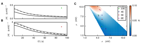
Figure 10: A Absolute value of dynamic transfer function $H$ for $(\mu,\sigma)_{2/3E}=(3.9,5.0)\,\mathrm{mV}$ (black), $(\mu,\sigma)=(4.4,5.0)\,\mathrm{mV}$ (gray) and $H^{approx}$ (black, dashed). Other parameters are $\tau_{m}=10\,\mathrm{ms}$, $\tau_{\mathrm{syn}}=0.5\,\mathrm{ms}$, $V_{\theta}=-55\,\mathrm{mV}$ and $V_{R}=-70\,\mathrm{mV}$. Parameters correspond to population 2/3E (green cross in C). B Absolute value of dynamical transfer function $H$ for $(\mu,\sigma)_{5I}=(9.3,4.5)\,\mathrm{mV}$ (black), (gray) $(\mu,\sigma)=(9.8,4.5)\,\mathrm{mV}$ and $H^{approx}$(black, dashed). Parameters correspond to population 5I (red cross in C). C Relative error $R(\mu,\sigma,\mu^{\prime})$ of the approximation given by Eq (44) for $\delta\mu=0.5\,\mathrm{mV},\,\omega_{max}=2\pi\cdot 200\,\mathrm{Hz}$. Choice of $\delta\mu$ corresponds to a relative change of the rate $r_{0}$ of $25$ percent on average. Qualitatively similar results are obtained for different values of $\delta\mu$, where the error $R$, in general, increases with increasing $\delta\mu$. Values of $\mu$ and $\sigma$ are constrained to regions in which the resulting stationary rate $r_{0}$ is in the range $r_{0}\in(0.1\,\mathrm{Hz},10\,\mathrm{Hz})$. Since the static transfer function is strictly increasing with $\sigma$ the left edge of the shown region corresponds to $r_{0}=0.1\,\mathrm{Hz}$ and the right edge to $r_{0}=10\,\mathrm{Hz}$. The working points for the $8$ populations of the microcircuit are marked with symbols (see legend, crosses mark respective inhibitory populations).

We therefore neglect the variation of $\sigma$ and restrict the analysis to a perturbation of the mean, i.e. $\mu\rightarrow\mu^{\prime}=\mu+\delta\mu$. Fig 10A shows that the DC limit of $H$ significantly changes while its shape stays approximately constant. This suggests that we can approximate $H(\omega,\mu^{\prime},\sigma)$ by a change of the DC-limit by altering the prefactor in the following way

$$H(\omega,\mu^{\prime},\sigma) \approx \frac{A(\mu^{\prime},\sigma)}{A(\mu,\sigma)}\,H(\omega,\mu,\sigma)=:H^{approx}(\omega,\mu,\mu^{\prime},\sigma).$$ (42)

In the approximation above a change in the input yields the following dynamic transfer function

$$H_{I}(\omega) =H(\omega,\mu^{\prime},\sigma)=\left(1+\frac{\delta A(\mu,\mu^{\prime},\sigma)}{A(\mu,\sigma)}\right)H(\omega,\mu,\sigma)$$

$$\mbox{with}\quad\delta A(\mu,\mu^{\prime},\sigma)=\frac{\partial^{2}\nu}{\partial\mu^{2}}\,\delta\mu.$$ (43)

This approximation can be evaluated defining the relative error

$$R(\mu,\sigma,\mu^{\prime}) = \frac{\int_{0}^{\omega_{max}}(|H^{approx}(\omega,\mu,\mu^{\prime},\sigma)|-|H(\omega,\mu^{\prime},\sigma)|)d\omega}{\int_{0}^{\omega_{max}}(|H(\omega,\mu^{\prime},\sigma)|)d\omega},$$ (44)

which is shown in Fig 10C. In the fluctuation driven regime, which corresponds to low values of $\mu$ and high values of $\sigma$ (bottom part of the figure), $H^{approx}$ constitutes a good approximation. In the regime with large $\mu$ and low $\sigma$ the approximation $H^{approx}$ is less accurate since the change in the shape of $H$ is not negligible (Fig 10B), in line with the finding of a resonance at the firing rate in the mean driven regime [5].

In conclusion, in the fluctuation driven regime the perturbation can be approximately absorbed into the prefactor of the dynamic transfer function. Note that the DC-limit does not change for variations of $\mu$ that affect the static transfer function $\nu(\mu,\sigma)$ in the linear regime, where $\partial\nu(\mu,\sigma)/\partial\mu$ is constant by definition. However, it turns out that the static transfer functions of the populations with working points equal to those in the microcircuit model (shown in 10C) are affected nonlinearly by a perturbation in $\mu$ ($\partial^{2}\nu(\mu,\sigma)/\partial\mu^{2}\neq 0$).

So far, populations were considered in isolation. To investigate how a perturbation effects the dynamic transfer function of a population embedded into a network, we now treat a perturbation of the mean external input $\mu_{\mathrm{ext}}$ to a population in the microcircuit model. Since the stationary rates of the populations in the network depend on each other, the static transfer function needs to be solved self-consistently when introducing a perturbation to one population. This yields a new stationary rate $r_{0}^{\prime}=r_{0}+\delta r_{0}$ and working point for each population. We first investigate the induced changes in the rates (Fig 11A). A perturbation to one population has an effect on all eight populations, where by trend a positive perturbation to an excitatory population causes an increase in the rates while the opposite is true for a perturbation of an inhibitory population (compare $\mathrm{pop_{\mathrm{pert}}}=\mathrm{4E}/4I$). However, increased input can also yield higher rates in some populations and lower ones in others (see $\mathrm{pop_{\mathrm{pert}}}=6E$ and $\mathrm{pop_{\mathrm{pert}}}=6I$). Another tendency is that excitatory populations are more strongly affected by perturbations than inhibitory ones. In particular, population 5E is very sensitive to perturbations of populations in L4 or L5, while populations in L4 are very sensitive to perturbations in L4.

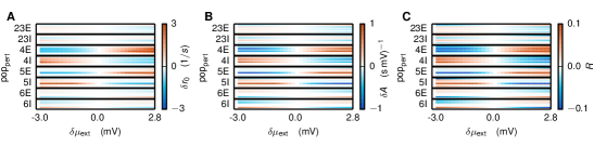
Figure 11: Perturbation of the input to the microcircuit. A One block of eight rows shows the change in the stationary rate $\delta r_{0}$ of the populations in the microcircuit in response to a perturbation $\delta\mu_{\mathrm{ext}}$ to population $\mathrm{pop}_{\mathrm{pert}}$, as specified on the y-axis. Each individual block is ordered from top to bottom according to the populations [2/3E, 2/3I, 4E, 4I, 5E, 5I, 6E, 6I] with black rows separating the blocks. For example, the second line in the top row shows the change in the stationary rate of population 2/3I after perturbing the external input to population 2/3E. The range of $\delta\mu_{\mathrm{ext}}$ corresponds roughly to a change of the external rate ($r_{\mathrm{ext}}=8\,\mathrm{Hz})$ of about $\pm 1\,\mathrm{Hz}$ B Changes of the DC-limit to perturbation. Structure as in A. C: Changes of the error $R$ to perturbation. Structure as in A.

We further investigate the corresponding changes in the DC-limit of the dynamic transfer function (Fig 11B). In general the DC-limit follows the changes of the rates. However, some differences can be observed: for example when perturbing population 4E the rate of population 5I is sensitive to the perturbation, but the DC-limit stays almost constant, which hints on the perturbation acting on the linear regime of the static transfer function of population 5I. In summary, comparing the response of a population in isolation and embedded in a network to a perturbation in its input shows that the network structure can amplify or decrease as well as reverse the sign of the response. The responses of the other populations to this perturbation can be uniform as well as diverse.

The relative error, which here needs to account for both, the change in $\mu$ as well as the change in $\sigma$ induced by rate changes of the other populations (compared to Eq (44) which does not depend on changes in $\sigma$), reads

$$R(\mu,\sigma,\mu^{\prime}) = \frac{\int_{0}^{\omega_{max}}(|H^{approx}(\omega,\mu,\mu^{\prime},\sigma,\sigma^{\prime})|-|H(\omega,\mu^{\prime},\sigma^{\prime})|)d\omega}{\int_{0}^{\omega_{max}}(|H(\omega,\mu^{\prime},\sigma^{\prime})|)d\omega}$$

and is shown in Fig 11C. The error follows the behavior of the rate and the DC-limit and therefore shows that the higher the changes in the working point of the populations the higher the error. The error of the approximation of the dynamic transfer functions is large compared to the error for the same populations in isolation. However, it stays within the limits of $10\%$ given an alteration of the input of the same order. How these changes effect the prediction of the spectrum remains to be investigated.

Mapping changes in the stationary rate to changes in the eigenvalue

We identify the eigenvalue trajectory of the one-dimensional circuit (discussed in “Dynamic responses of a self-coupled inhibitory population”) as the weighted dynamic transfer function

$$\lambda(\omega)=-wH(\omega),$$ (45)

where $\lambda(\omega)$ denotes the Fourier transformation of the time dependent eigenvalue defined as $\tilde{\lambda}(t)=\frac{1}{2\pi}\int\lambda(\omega)\,e^{i\omega t}\,d\omega$. The eigenvalue trajectory of the circuit with an additional large constant input reads

$$\lambda_{I}(\omega)=-wH_{I}(\omega)\approx-w(1+\delta A/A)H(\omega),$$ (46)

where we inserted the approximation of the dynamical transfer function, which is discussed in the previous section. Changes in the eigenvalue can therefore be parameterized as

$$\lambda_{I}=(1+\alpha_{\lambda})\lambda,$$

with $\alpha_{\lambda}=\delta A/A$ being the ratio by which the prefactor of the dynamic transfer function is shifted and which is related to the excitability of the circuit (Fig 1). The frequency dependence of the eigenvalues was omitted for clarity of notation. The following considerations show how the shift in the eigenvalue relates to the change of the stationary rate.

A constant stimulus is applied by an increase in the external rate ($\tilde{\nu}_{\mathrm{ext}}=(1+\alpha_{\mu})\nu_{\mathrm{ext}}$), yielding a change in the mean value of the input current ($\delta\mu_{\mathrm{ext}}=\alpha_{\mu}\mu_{ext}$, see Eq (41)). Following the argument in the previous section, we neglect changes in the variance. The change in the external input yields the following change in the stationary rate $r_{0}$

$$\alpha_{r}r_{0}=\left.\frac{\partial\nu}{\partial\mu}\right|_{\mu=\mu_{\mathrm{ext}}}\delta\mu+\frac{1}{2}\left.\frac{\partial^{2}\nu}{\partial\mu^{2}}\right|_{\mu=\mu_{\mathrm{ext}}}\delta\mu^{2},$$ (47)

where higher orders in the derivative of the static transfer function $\nu(\mu,\sigma)$ were neglected. In this recurrent network $\delta\mu$ is composed of the perturbation in the external input $\delta\mu_{\mathrm{ext}}$ in addition to a contribution from the feedback connection $\delta\mu_{\mathrm{\mathrm{rec}}}=-wr_{0}$. We now identify that $A=\left.\frac{\partial\nu}{\partial\mu}\right|_{\mu=\mu_{\mathrm{ext}}}$, abbreviate $m=\left.\frac{\partial^{2}\nu}{\partial\mu^{2}}\right|_{\mu=\mu_{\mathrm{ext}}}$and recall that $\delta A=m\delta\mu$ (Eq (43)). Inserting this in the equation above yields the following relation between the ratio of the eigenvalue shift and the rate change

$$\frac{\left(\alpha_{\lambda}+1\right)^{2}-1}{2\alpha_{r}}=\frac{r_{0}m}{A^{2}}.$$ (48)

This shows that in this approximation the eigenvalue does not shift, if the working point sets the static transfer function in the linear regime, i.e. $m=0$. However, we demonstrated that, in particular, in recurrent networks the nonlinear effect can play a role (Fig 11).

For the self-coupled inhibitory units (discussed in “Dynamic responses of a self-coupled inhibitory population”), we chose the following parameters:

$$\alpha_{\lambda} =0.15\>,r_{0}/N=1\,\mathrm{Hz},\>\alpha_{r}=0.8,\>w=-4\>mV$$

$$\mathrm{\mbox{yielding}}\quad A=0.05\>\mathrm{mV}^{-1},\>A_{I}=0.058\>\mathrm{mV}^{-1}$$

$$\mbox{and}\quad\tau=2\,\mathrm{ms},\>d=3.6\,\mathrm{ms},\>I_{0}=0.5/\pi.$$ (49)

The parameters of the dynamic transfer function for both populations in the two-dimensional circuits (discussed in “Stimulus evoked spectra in a two dimensional network”) are given by:

$$r_{0,\mathrm{E}}/N_{\mathrm{E}} =r_{0,I}/N_{\mathrm{I}}=1\,\mathrm{Hz},\>A=0.5\>\mathrm{mV}^{-1},\>w=1\,\mathrm{mV}$$

$$\tau =2\,\mathrm{ms},\>d=1.5\,\mathrm{ms},\>I_{0}=0.5/\pi.$$ (50)

Composition of the spectrum

The systems considered in this work are given by, or can be reduced to, $N$-dimensional rate models with noise, while $N$ denotes the number of populations. The spectrum of the populations is hence identical to the diagonal of

$$\mathbf{C}(\omega)=\langle\mathbf{Y}(\omega)\mathbf{Y}^{\mathrm{T}}(-\omega)\rangle,$$ (51)

where $\mathbf{Y}(\omega)$ is the rate vector in Fourier space, composed of the rate $\mathbf{R}(\omega)$ and a noise term $\mathbf{X}(\omega)$ as $\mathbf{Y}(\omega)=\mathbf{R}(\omega)+\mathbf{X}(\omega)$. Inserting the effective connectivity matrix, which is composed of the connection strengths $M_{ij}$ and the dynamical transfer function of the populations incorporating the connection delays $H_{i}(\omega)e^{-i\omega d_{ij}}$(for further detail see [34]) into the self-consistent equation for the population rates (Eq (39)), yields

$$\mathbf{C}(\omega)=(\mathbb{I}-\tilde{\mathbf{M}}_{\mathrm{d}}(\omega))^{-1}\,\mathbf{D}\,(\mathbb{I}-\tilde{\mathbf{M}}_{\mathrm{d}}(-\omega))^{-1,\mathrm{T}},$$ (52)

with the diagonal matrix $\mathbf{D}=\langle\mathbf{X}(\omega)\mathbf{X}^{\mathrm{T}}(-\omega)\rangle$ describing the power spectrum of the noise. In the reduction of spiking networks, the noise is a finite-size effect with the autocovariance $D_{ii}=\bar{r}_{i}/N_{i}\equiv r_{i}$ , where $\bar{r}_{i}$ is the stationary firing rate of the $i$-th population and $N_{i}$ the number of neurons within population $i$.

The eigenvectors and eigenvalues of the effective connectivity matrix are defined as

$$\tilde{\mathbf{M}}_{d}(\omega)\mathbf{u}_{i}(\omega) =\lambda_{i}(\omega)\mathbf{u}_{i}(\omega)$$

$$\mathbf{v}_{i}^{T}(\omega)\tilde{\mathbf{M}}_{d}(\omega) =\lambda_{i}(\omega)\mathbf{v}_{i}^{\mathrm{T}}(\omega).$$ (53)

The eigenvectors $\mathbf{u}_{i}(\omega)$ and $\mathbf{v}_{i}(\omega)$ with the convention $|\mathbf{u}_{i}(\omega)|^{2}=1$ and $\mathbf{v}_{i}^{\mathrm{T}}(\omega)\mathbf{u}_{j}(\omega)=\delta_{ij}$ constitute a bi-orthogonal basis. The eigenvectors and eigenvalues of the term $(\mathbb{I}-\tilde{\mathbf{M}}_{\mathrm{d}}(\omega))^{-1}$ appearing in Eq (52) are given by

$$(\mathbb{I}-\tilde{\mathbf{M}}_{\mathrm{d}}(\omega))^{-1}\mathbf{u}_{i}(\omega) =\frac{1}{1-\lambda_{i}(\omega)}\mathbf{u}_{i}(\omega)$$

$$\mathbf{v}_{i}^{\mathrm{T}}(\omega)(\mathbb{I}-\tilde{\mathbf{M}}_{\mathrm{d}}(\omega))^{-1} =\frac{1}{1-\lambda_{i}(\omega)}\mathbf{v}_{i}^{\mathrm{T}}(\omega).$$ (54)

The diagonal noise correlation matrix $\mathbf{D}$ can be written as the sum of outer products of the unit vectors $\mathbf{e}_{i}$, which have the entry one at position $i$ and zero everywhere else, weighted by the diagonal entries $r_{i}$

$$\mathbf{D}=\sum_{i}r_{i}\mathbf{e}_{i}\mathbf{e}_{i}^{\mathrm{T}}.$$ (55)

The unit vectors can be rewritten in the basis spanned by the eigenvectors of the effective connectivity matrix

$$\mathbf{e}_{i}=\sum_{j}\alpha_{j}^{i}(\omega)\mathbf{u}_{j}(\omega)\,\mbox{with}\>\alpha_{j}^{i}(\omega)=\mathbf{v}_{j}^{\mathrm{T}}(\omega)\mathbf{e}_{i}.$$ (56)

Here $\alpha_{j}^{i}(\omega)$ describes the projection of the $i$-th unit vector onto the $j$-th eigenmode. Inserting the decomposition of the unit vectors (Eq (56)) into Eq (55) yields the noise correlation matrix in the new basis

$$\mathbf{D}=\sum_{n,m}\beta_{nm}(\omega)\mathbf{u}_{n}(\omega)\mathbf{u}_{m}^{\mathrm{T}*}(\omega),$$ (57)

with $\beta_{nm}(\omega)=\sum_{i}r_{i}\alpha_{n}^{i}(\omega)\alpha_{m}^{i*}(\omega)$ weighing the $i$-th component of the $n$-th and $m$-th left eigenvector with the rate of the $i$-th population. In other words, the $i$-th population has a large contribution to $\beta_{nm}(\omega)$ if the unit vector of population $i$ points in a similar direction as the right eigenvector of the $n$-th and $m$-th mode and population $i$ has a large rate $r_{i}$. Here we also used that the effective connectivity matrix is real valued in the time domain and therefore has the property $\tilde{M}(-\omega)=\tilde{M}(\omega)^{\ast}$ in Fourier domain. Inserting Eq (57) and the effective connectivity matrix in the new basis (Eq (54)) into the expression for the spectrum (Eq (52)) results in

$$\mathbf{C}(\omega) =\Big{(}\sum_{n}\frac{1}{1-\lambda_{n}(\omega)}\mathbf{u}_{n}(\omega)\mathbf{v}_{n}^{T}(\omega)\Big{)}\Big{(}\sum_{j,k}\beta_{jk}(\omega)\mathbf{u}_{j}(\omega)\mathbf{u}_{k}^{T*}(\omega)\Big{)}$$

$$\quad\>\Big{(}\sum_{m}\frac{1}{1-\lambda_{m}^{*}(\omega)}\mathbf{v}_{m}^{*}(\omega)\mathbf{u}_{m}^{T*}(\omega)\Big{)}$$

$$=\sum_{n,m}\frac{\beta_{nm}(\omega)}{(1-\lambda_{n}(\omega))(1-\lambda_{m}^{*}(\omega))}\mathbf{u}_{n}(\omega)\mathbf{u}_{m}^{T*}(\omega).$$ (58)

The spectrum of the eight dimensional microcircuit is hence composed of $64$ contributions. Eight contributions arise from individual modes ($n=m$) and the remaining terms arise from contributions of pairs of different modes ($n\neq m$).

Composition of the spectrum with input

So far the contribution of external input on the spectrum produced by the circuit has been neglected. In the microcircuit, all model neurons receive external Poisson input from a population-specific number of independent sources that each fire with the rate $\nu_{\mathrm{ext}}=8\,\mathrm{Hz}$. Given that all $N_{\mathrm{ext},i}$ external sources are independent, the total Poisson input received by the $j$th neuron in the $i$th population can be approximated by Gaussian white noise described by

$$y_{\mathrm{ext},i}^{j}(t) =\sum_{k=1}^{N_{\mathrm{ext},i}}\left(\nu_{\mathrm{ext}}+\sqrt{\nu_{\mathrm{ext}}}\chi_{\mathrm{ext},i}^{jk}(t)\right)=N_{\mathrm{ext},i}\nu_{\mathrm{ext}}+\sum_{k=1}^{N_{\mathrm{ext},i}}\sqrt{\nu_{\mathrm{ext}}}\chi_{\mathrm{ext},i}^{jk}(t)$$

$$=N_{\mathrm{ext},i}\nu_{\mathrm{ext}}+\sqrt{N_{\mathrm{ext},i}\nu_{\mathrm{ext}}}\chi_{\mathrm{ext},i}^{j}(t).$$ (59)

Here $\chi_{\mathrm{ext},i}^{jk}(t)$ is a random variable with zero mean ($\langle\chi_{\mathrm{ext},i}^{jk}(t)\rangle=0$) and variance $\langle\chi_{\mathrm{ext},i}^{jk}(t)\chi_{\mathrm{ext},i^{\prime}}^{j^{\prime}k^{\prime}}(t^{\prime})\rangle=\delta_{ii^{\prime}}\,\delta_{kk^{\prime}}\,\delta_{jj^{\prime}}\,\delta(t-t^{\prime})$. The last equal sign in Eq (59) follows from the fact that two Gaussian white noise processes are equal if they have equal first and second moments. The population averaged input of the $i$th population is given by

$$y_{\mathrm{ext},i}(t) =\frac{1}{M_{i}}\sum_{j=1}^{M_{i}}\left(N_{\mathrm{ext},i}\nu_{\mathrm{ext}}+\sqrt{N_{\mathrm{ext},i}\nu_{\mathrm{ext}}}\chi_{\mathrm{ext},i}^{j}(t)\right)$$

$$=N_{\mathrm{ext},i}\nu_{\mathrm{ext}}+\frac{1}{M_{i}}\sum_{j=1}^{M_{i}}\sqrt{N_{\mathrm{ext},i}\nu_{\mathrm{ext}}}\chi_{\mathrm{ext},i}^{j}(t)$$

$$=N_{\mathrm{ext},i}\nu_{\mathrm{ext}}+\sqrt{\frac{N_{\mathrm{ext},i}\nu_{\mathrm{ext}}}{M_{i}}}\chi_{\mathrm{ext},i}(t),$$ (60)

where $M_{i}$ is the number of neurons in population $i$. The statistics of the input therefore does not depend on whether each population receives input form several Poisson sources with low firing rates or one Poisson source with high firing rate.

When the firing rate of the external input is modulated in time $\nu_{\mathrm{ext}}(t)=\nu_{\mathrm{ext}}f(t)$, a neuron in population $i$ receives Gaussian white noise with time dependent mean and variance

$$y_{\mathrm{ext},i}(t)=\mu_{\mathrm{ext},i}(t)+\sigma_{\mathrm{ext},i}(t)\chi_{\mathrm{ext},i}(t),$$ (61)

with $\mu_{\mathrm{ext},i}(t)=N_{\mathrm{ext},i}\nu_{\mathrm{ext}}(t)$ and $\sigma_{\mathrm{ext},i}(t)=\sqrt{N_{\mathrm{ext},i}\nu_{\mathrm{ext}}(t)/M_{i}}$. The description introduced here is valid around one working point of the populations and therefore for fluctuations around one stationary firing rate. Motivated by this, we choose $f(t)$ to describe a modulation around the external rate, which does not change its original value when averaged over long time series, i.e. $\underset{T\rightarrow\infty}{\mathrm{lim}}\frac{1}{2T}\int_{-T}^{T}\nu_{\mathrm{ext}}(t)dt=\nu_{\mathrm{ext}}$.

Incorporating the external input into the self-consistency of the rate fluctuations (Eq (39)) yields

$$r_{i}(t)=h_{i}\ast\sum_{j=1}^{N}M_{ij}^{A}y_{j}(\circ-d_{ij})+\tau_{m}J_{\mathrm{ext}}\left[h_{i}\ast y_{\mathrm{ext},i}(\circ)\right](t),$$ (62)

with the strength of the external current $w_{ext}$ ($J_{\mathrm{ext}}=\tau_{\mathrm{syn}}w_{\mathrm{ext}}/C_{m}$) in Ampere, which is chosen to equal the synaptic strength within the network as defined in Eq (35). Defining the effective connectivity matrix $\tilde{\mathbf{M}}_{\mathrm{d}}(\omega)$ to incorporate the convolution of the dynamic transfer function $h_{i}$ and the anatomical connectivity $M_{ij}^{\mathrm{A}},$ as well as the delays and delay distribution [34], the fluctuating rate of the circuit reads in Fourier space

$$\mathbf{Y}(\omega)=\tilde{\mathbf{M}}_{\mathrm{d}}(\omega)\mathbf{\mathbf{Y}}(\omega)+\mathbf{D}_{\mathrm{ext}}(\omega)\mathbf{Y}_{\mathrm{ext}}(\omega)+\mathbf{X}(\omega)$$

$$\Leftrightarrow \mathbf{Y}(\omega)=\mathbf{P}(\omega)\left(\mathbf{D}_{\mathrm{ext}}(\omega)\mathbf{Y}_{\mathrm{ext}}(\omega)+\mathbf{X}(\omega)\right),$$ (63)

where the eigenvalues and eigenvectors of $\mathbf{P}(\omega)=(\mathbb{I}-\tilde{\mathbf{M}}_{\mathrm{d}}(\omega))^{-1}$ are defined in Eq (54) and $\mathbf{D}_{\mathrm{ext}}(\omega)$ is a diagonal matrix with elements $D_{\mathrm{ext},ii}(\omega)=\tau_{m}J_{\mathrm{ext}}H_{i}(\omega)$. The population rate spectra read

$$\mathbf{C}_{\mathrm{I}}(\omega) =\langle\mathbf{Y}(\omega)\mathbf{Y}^{T}(-\omega)\rangle$$

$$=\underset{=\mathbf{C}_{0}(\omega)}{\underbrace{\mathbf{P}(\omega)\langle\mathbf{X}(\omega)\mathbf{X}^{T}(-\omega)\rangle\mathbf{P}^{T}(-\omega)}}+\underset{=\mathbf{C}_{\mathrm{ext}}(\omega)}{\underbrace{\mathbf{P}(\omega)\mathbf{D}_{\mathrm{ext}}(\omega)\langle\mathbf{Y}_{\mathrm{ext}}(\omega)\mathbf{Y}_{\mathrm{ext}}^{T}(-\omega)\rangle\mathbf{D}_{\mathrm{ext}}^{T}(-\omega)\mathbf{P}^{T}(-\omega)}},$$ (64)

where we used that the internal and external noise sources have zero mean and we assumed them to be uncorrelated. The spectrum observed in the circuit is thus given by the spectrum generated within the circuit (Eq (52)) and the spectrum imposed from the outside $\mathbf{C}_{\mathrm{ext}}(\omega)$. Before calculating the expectation value of the external fluctuations $\langle\mathbf{Y}_{\mathrm{ext}}(\omega)\mathbf{Y}_{\mathrm{ext}}^{T}(-\omega)\rangle$, we notice that the autocorrelation of the signal defined in Eq (61) depends on two time arguments, namely the time-lag $\tau$ as well as the global time $t$, which is induced by the modulation of the rate

$$\langle y_{\mathrm{ext},i}(t)y_{\mathrm{ext},j}(t+\tau)\rangle =N_{\mathrm{ext},i}N_{\mathrm{ext},j}\nu_{\mathrm{ext}}^{2}f_{i}(t)f_{j}(t+\tau)+\delta_{ij}\delta(\tau)\,\frac{N_{\mathrm{ext},i}\nu_{\mathrm{ext}}}{M_{i}}f_{i}(t),$$ (65)

where we used that $\langle\chi_{\mathrm{ext},i}(t)\chi_{\mathrm{ext},j}(t+\tau)\rangle=\delta_{ij}\delta(\tau)$. The autocorrelation is modulated in time and the process is therefore not stationary. The time dependent spectral density, also known as the Wigner-Ville spectrum (GWVS) [54] is given by

$$\langle\mathbf{Y}_{\mathrm{ext}}(\omega,t)\mathbf{Y}_{\mathrm{ext}}^{T}(-\omega,t)\rangle_{ij} =\int_{-\infty}^{\infty}e^{-i\omega\tau}\langle y_{\mathrm{ext},i}(t)y_{\mathrm{ext},j}(t+\tau)\rangle d\tau$$

$$\overset{t^{\prime}=t+\tau}{=}N_{\mathrm{ext},i}N_{\mathrm{ext},j}\nu_{\mathrm{ext}}^{2}f_{i}(t)e^{i\omega t}\underset{T\rightarrow\infty}{\mathrm{lim}}\int_{-T}^{T}e^{-i\omega t^{\prime}}f_{j}(t^{\prime})\,dt^{\prime}$$

$$\quad\quad\>+\delta_{ij}\delta(\tau)\,\frac{N_{\mathrm{ext},i}\nu_{\mathrm{ext}}}{M_{i}}\,f_{i}(t)$$

$$=N_{\mathrm{ext},i}N_{\mathrm{ext},j}\nu_{\mathrm{ext}}^{2}f_{i}(t)e^{i\omega t}F_{j}(\omega)+\delta_{ij}\delta(\tau)\frac{N_{\mathrm{ext},i}\nu_{\mathrm{ext}}}{M_{i}}f_{i}(t),$$ (66)

where $F(\omega)$ denotes the Foureir transform of $f(t)$. The GWVS describes the time-frequency distribution of the mean energy of the signal $y_{\mathrm{ext}}(t)$. The normalized marginal distribution can be obtained by taking the average over time

$$\langle\mathbf{Y}_{\mathrm{ext}}(\omega)\mathbf{Y}_{\mathrm{ext}}^{T}(-\omega)\rangle_{ij} =\underset{T\rightarrow\infty}{\mathrm{lim}}\frac{1}{2T}\int_{-T}^{T}\langle\mathbf{Y}_{\mathrm{ext}}(\omega,t)\mathbf{Y}_{\mathrm{ext}}^{T}(-\omega,t)\rangle_{ij}dt$$

$$=\mu^{2}F_{i}(\omega)\underset{T\rightarrow\infty}{\mathrm{lim}}\frac{1}{2T}\int_{-T}^{T}f_{j}(t)e^{i\omega t}dt+\sigma^{2}\underset{T\rightarrow\infty}{\mathrm{lim}}\frac{1}{2T}\int_{-T}^{T}f_{i}(t)dt$$

$$=N_{\mathrm{ext},i}N_{\mathrm{ext},j}\nu_{\mathrm{ext}}^{2}\underset{T\rightarrow\infty}{\mathrm{lim}}\frac{1}{2T}F_{i}^{*}(\omega)F_{j}(\omega)$$

$$\quad+\delta_{ij}\frac{N_{\mathrm{ext},i}\nu_{\mathrm{ext}}}{M_{i}}\underset{T\rightarrow\infty}{\mathrm{lim}}\frac{1}{2T}\int_{-T}^{T}f_{i}(t)dt$$

$$=N_{\mathrm{ext},i}N_{\mathrm{ext},j}\nu_{\mathrm{ext}}^{2}\underset{T\rightarrow\infty}{\mathrm{lim}}\frac{1}{2T}F_{i}^{*}(\omega)F_{j}(\omega)+\delta_{ij}\frac{N_{\mathrm{ext},i}\nu_{\mathrm{ext}}}{M_{i}},$$ (67)

where the last integral could be discarded since we required that the time dependent modulation of the firing rate $f_{i}(t)$ averages out over long time series. The terms above show that a modulation of the external firing rates yields two contributions to the spectrum. The first term describes the contribution that arises from the modulation of the mean, which can give rise to new peaks. In the original microcircuit model, the external rate is constant ($f_{i}(t)=1$). The first term thus solely gives a contribution at zero frequency ($F_{i}(\omega)=2\pi\delta(\omega)$). The second term describes the effect of the modulation of the variance. This term cannot introduce new peaks in the spectrum, since it does not depends on $\omega$. It, however, gives a contribution at all frequencies and can therefore influence the amplification of the dynamical modes of the systems. The contribution of the external variance is large compared to the variance of the noise generated within the network, which is of order $\nu_{\mathrm{ext}}/M_{i}$. However, its contribution is negligible, since it is small for in the microcircuit model and additionally filtered out by the transfer function of the population for larger frequencies (see definition of $\mathbf{D}_{\mathrm{ext}}(\omega)$ and Eq (64)). In the following we will therefore focus on the dynamical contribution of the first term.

Let us now assume that the fraction $a$ of the external input to the $k$th population is modulated by a sinusoid of frequency $\omega_{\mathrm{I}}$ such that $f(t)=1+a\>\sin(\omega_{\mathrm{I}}t)$ yielding the modulated mean and variance

$$\mu_{\mathrm{ext},k}(t) =N_{\mathrm{ext},k}\nu_{\mathrm{ext}}\left(1+a\,\sin(\omega_{\mathrm{I}}t)\right)$$

$$\sigma_{\mathrm{ext},k}^{2}(t) =\frac{N_{\mathrm{ext},k}}{M_{k}}\nu_{\mathrm{ext}}\left(1+a\,\sin(\omega_{\mathrm{I}}t)\right),$$ (68)

while all other populations receive unmodulated external input. The contribution of the mean modulation to the spectrum of the external signal is then, for $\omega>0$, given by

$$\langle\mathbf{Y}_{\mathrm{ext}}(\omega)\mathbf{Y}_{\mathrm{ext}}^{T}(-\omega)\rangle_{ij}=\begin{cases}N_{\mathrm{ext},k}^{2}\nu_{\mathrm{ext}}^{2}\underset{T\rightarrow\infty}{\mathrm{lim}}\frac{1}{2T}a^{2}\pi^{2}\left(\delta^{2}(\omega-\omega_{\mathrm{I}})+\delta^{2}(\omega+\omega_{\mathrm{I}})\right)&\mbox{for}\>i=j=k\\ 0&\mbox{else.}\end{cases}$$ (69)

Thus the spectrum exhibits a $\delta$-peak at the frequency of the modulating signal. To determine the height of the peak, we consider that the measurement or the modulation lasts only a finite duration. Inserting the definition of the $\delta$-function $2\pi\delta(\omega-\omega_{\mathrm{I}})=\underset{T\rightarrow\infty}{\mathrm{lim}}\int_{-T}^{T}e^{-i(\omega-\omega_{\mathrm{I}})\tau}d\tau$, the peak height at $\omega_{\mathrm{I}}$, when measured in the interval $[0,T]$ (which changes the normalization constant in Eq (69) from $1/2T$ to $1/T$), is given by

$$\underset{\omega\rightarrow\omega_{\mathrm{I}}}{\mathrm{lim}}\delta_{T}(\omega-\omega_{\mathrm{I}})=\frac{1}{2\pi}\underset{\omega\rightarrow\omega_{\mathrm{I}}}{\mathrm{lim}}\int_{0}^{T}e^{-i(\omega-\omega_{\mathrm{I}})\tau}d\tau=\frac{1}{2\pi}\underset{\omega\rightarrow\omega_{\mathrm{I}}}{\mathrm{lim}}\frac{e^{-i(\omega-\omega_{\mathrm{I}})T}-1}{-i(\omega-\omega_{\mathrm{I}})}=\frac{T}{2\pi},$$ (70)

yielding the following spectrum of the external signal

$$\langle\mathbf{Y}_{\mathrm{ext}}(\omega)\mathbf{Y}_{\mathrm{ext}}^{T}(-\omega)\rangle_{ij}=\begin{cases}N_{\mathrm{ext},k}^{2}\nu_{\mathrm{ext}}^{2}a^{2}\frac{T}{4}&\mbox{for}\>i=j=k\>\mbox{and }\>\omega=\omega_{\mathrm{I}}\\ 0&\mbox{else.}\end{cases}$$ (71)

The additional contribution to the spectrum visible in the network due to the external input is therefore given by

$$C_{\mathrm{ext},ij}(\omega) =\sum_{n,m}P_{in}(\omega)D_{\mathrm{ext},nn}(\omega)\langle Y_{\mathrm{ext}}(\omega)Y_{\mathrm{ext}}^{T}(-\omega)\rangle_{nm}D_{\mathrm{ext},mm}(-\omega)P_{jm}(-\omega)$$ (72)

yielding

$$\mathbf{C}_{\mathrm{ext}}(\omega)=\begin{cases}w_{\mathrm{ext}}^{2}N_{\mathrm{ext},k}^{2}\nu_{\mathrm{ext}}^{2}a^{2}\frac{T}{4}\left|H_{k}(\omega)\right|^{2}\mathbf{P}(\omega)\mathbf{P}^{T}(-\omega)&\mbox{for}\>\omega=\omega_{\mathrm{I}}\\ 0&\mbox{else.}\end{cases}$$ (73)

The expression above shows that the peak imposed on one population from the outside is propagated through the network and is therefore visible in all populations. The height of the peaks scales linearly with time.

As opposed to the above described current modulation, rate modulating input is directly added on top of the population rate and not filtered by the transfer function of the population, yielding the following additive term in the spectrum

$$\mathbf{C}_{\mathrm{ext}}^{\mathrm{RM}}(\omega)=\begin{cases}w_{\mathrm{ext}}^{2}N_{\mathrm{ext},k}^{2}\nu_{\mathrm{ext}}^{2}a^{2}\frac{T}{4}\mathbf{P}(\omega)\mathbf{P}^{T}(-\omega)&\mbox{for}\>\omega=\omega_{\mathrm{I}}\\ 0&\mbox{else.}\end{cases}$$ (74)

Analyzing the current modulating input further by decomposing the externally imposed spectrum, when population $k$ is stimulated in the eigenbasis of the propagator matrix, as already done for the internally generated spectrum Eq (58), yields

$$\mathbf{D}_{\mathrm{ext}}(\omega)\langle\mathbf{Y}_{\mathrm{ext}}(\omega)\mathbf{Y}_{\mathrm{ext}}^{T}(-\omega)\rangle\mathbf{D}_{\mathrm{ext}}(-\omega) =\sum_{n,km}\beta_{\mathrm{ext},nm}(\omega)\mathbf{u}_{n}(\omega)\mathbf{u}_{m}^{T*}(\omega)$$ (75)

with

$$\beta_{\mathrm{ext},nm}(\omega)=w_{\mathrm{ext}}^{2}N_{\mathrm{ext},k}^{2}\nu_{\mathrm{ext}}^{2}a^{2}\frac{T}{4}\left|H_{k}(\omega)\right|^{2}\alpha_{n}^{k}(\omega)\alpha_{m}^{k*}(\omega)$$ (76)

and $\alpha_{j}^{k}(\omega)=\mathbf{v}_{j}^{\mathrm{T}}(\omega)\mathbf{e}_{k}$. Inserting this into Eq (73) yields the decomposition of the population rate spectra at $\omega_{\mathrm{I}}$

$$\mathbf{C}_{\mathrm{I}}(\omega) =\sum_{n,m}\frac{\beta_{nm}(\omega)+\beta_{\mathrm{ext},nm}(\omega)}{(1-\lambda_{n}(\omega))(1-\lambda_{m}^{*}(\omega))}\mathbf{u}_{n}(\omega)\mathbf{u}_{m}^{\mathrm{T}*}(\omega).$$ (77)

The expression above is referred to as the response spectrum. The excess spectrum is defined as the additional power due to the input $\delta\mathbf{C}(\omega)=\mathbf{C}_{\mathrm{I}}(\omega)-\mathbf{C}_{0}(\omega)$. The power ratio, which describes the response spectrum at stimulus frequency $\omega_{\mathrm{I}}$ normalized by the original spectrum at that frequency, is evaluated at $\omega=\omega_{\mathrm{I}}$ and given by

$$\rho(\omega)=\frac{\mathbf{C}_{\mathrm{I}}(\omega)}{\mathbf{C}_{0}(\omega)}=1+\frac{\delta\mathbf{C}(\omega)}{\mathbf{C}_{0}(\omega)}.$$ (78)

Approximation of the LFP

The LFP is described as the input to pyramidal cells. The rate fluctuations received by pyramidal cells are given by

$$Y_{\mathrm{AMPA}}(\omega) =W_{\mathrm{E}\mathrm{E}}H_{\mathrm{AMPA}}(\omega)Y_{\mathrm{E}}(\omega)=\frac{ae^{-i\omega d}}{1+i\omega\tau_{\mathrm{AMPA}}}Y_{\mathrm{E}}(\omega)$$

$$Y_{\mathrm{GABA}}(\omega) =W_{\mathrm{E}\mathrm{I}}H_{\mathrm{GABA}}(\omega)Y_{\mathrm{I}}(\omega)=\frac{-be^{-i\omega d}}{1+i\omega\tau_{\mathrm{GABA}}}Y_{\mathrm{I}}(\omega),$$

where $\mathbf{Y}(\omega)=(Y_{\mathrm{E}}(\omega),Y_{\mathrm{I}}(\omega))$ denotes the vector of fluctuating rates of the excitatory and the inhibitory population. Here we assumed exponentially decaying synaptic currents with time constants $\tau_{\mathrm{AMPA}}$ and $\tau_{\mathrm{GABA}}$. The synaptic weights $a$ and $-b$ are defined in Eq (10). Mazzoni et al. [41] showed that the LFP is well approximated by the sum of absolute values of the currents received by the pyramidal neurons and is therefore given by

$$C_{\mathrm{LFP}}(\omega) =\langle\left(Y_{\mathrm{AMPA}}(\omega)-Y_{\mathrm{GABA}}(\omega)\right)\left(Y_{\mathrm{AMPA}}(-\omega)-Y_{\mathrm{GABA}}(-\omega)\right)\rangle$$

$$=\frac{a^{2}}{1+\omega^{2}\tau_{\mathrm{AMPA}}^{2}}\langle\left|Y_{\mathrm{E}}(\omega)\right|^{2}\rangle+\frac{b^{2}}{1+\omega^{2}\tau_{\mathrm{GABA}}^{2}}\langle\left|Y_{\mathrm{I}}(\omega)\right|^{2}\rangle$$

$$\quad+2ab\Re\left(\frac{\langle Y_{\mathrm{E}}(\omega)Y_{\mathrm{I}}(\omega)\rangle}{\left(1+i\omega\tau_{\mathrm{AMPA}}\right)\left(1-i\omega\tau_{\mathrm{GABA}}\right)}\right)$$

$$=\underset{\coloneqq C_{\mathrm{LFP}}^{\mathrm{auto}}(\omega)}{\underbrace{\frac{a^{2}}{1+\omega^{2}\tau_{\mathrm{AMPA}}^{2}}C_{\mathrm{E}\mathrm{E}}(\omega)+\frac{b^{2}}{1+\omega^{2}\tau_{\mathrm{GABA}}^{2}}C_{\mathrm{I}\mathrm{I}}(\omega)}}$$

$$\quad+\underset{\coloneqq C_{\mathrm{LFP}}^{\mathrm{cross}}(\omega)}{\underbrace{2ab\Re\left(\frac{C_{E\mathrm{I}}(\omega)}{\left(1+i\omega\tau_{\mathrm{AMPA}}\right)\left(1-i\omega\tau_{\mathrm{GABA}}\right)}\right)}}.$$ (79)

The LFP is thus determined by the autocorrelation of the rate fluctuations of each population as well as their crosscorrelation. The synaptic dynamics induces an additional low-pass filtering of the contributions. In this study we restrict the analysis of the LFP to $\delta$-synapses ($\tau_{\mathrm{AMPA}}=\tau_{\mathrm{GABA}}=0$) to isolate the phenomena induced by the static network structure.

References

- [1] Buzsaki G, Geisler C, Henze DA, Wang XJ. Interneuron Diversity series: Circuit complexity and axon wiring economy of cortical interneurons. TINS. 2004;27(4):186–193.
- [2] Buzsáki G, Wang XJ. Mechanisms of Gamma Oscillations. Annu Rev Neurosci. 2012;35:203–225.
- [3] Bartos M, Vida I, Jonas P. Synaptic mechanisms of synchronized gamma oscillations in inhibitory interneuron networks. natrevnsci. 2007;8:45–56.
- [4] Richardson MJE, Brunel N, Hakim V. From Subthreshold to Firing-Rate Resonance. J Neurophysiol. 2003 May;89(5):2538–2554. Available from: http://dx.doi.org/10.1152/jn.00955.2002.
- [5] Lindner B, Schimansky-Geier L. Transmission of noise coded versus additive signals through a neuronal ensemble. Phys Rev Lett. 2001;86:2934–2937.
- [6] Beltramo R, D’Urso G, Maschio MD, Farisello P, Bovetti S, Clovis Y, et al. Layer-specific excitatory circuits differentially control recurrent network dynamics in the neocortex. Nat Neurosci. 2013;16(2):227–234. Available from: http://dx.doi.org/10.1038/nn.3306.
- [7] Whittington MA, Traub RD, Kopell N, Ermentrout B, Buhl EH. Inhibition-based rhythms: experimental and mathematical observations on network dynamics. Int J Psychophysiol. 2000 December;38(3):315–336.
- [8] Binzegger T, Douglas RJ, Martin KAC. A Quantitative Map of the Circuit of Cat Primary Visual Cortex. J Neurosci. 2004;39(24):8441–8453.
- [9] Thomson AM, Lamy C. Functional maps of neocortical local circuitry. Front Neurosci. 2007;1(1):19–42.
- [10] Cardin JA, Carle M, Meletis K, Knoblich U, Zhang F, Deisseroth K, et al. Driving fast-spiking cells induces gamma rhythm and controls sensory responses. Nature. 2009;459(7247):663–667.
- [11] Destexhe A. How neuronal computations depend on network state: another piece in the puzzle. J Physiol (Lond). 2014;592:3339.
- [12] Altwegg-Boussac T, Chavez M, Mahon S, Charpier S. Excitability and responsiveness of rat barrel cortex neurons in the presence and absence of spontaneous synaptic activity in vivo. J Physiol (Lond). 2014;592:3577–95.
- [13] Fisahn A, Pike FG, Buhl EH, Paulsen O. Cholinergic induction of network oscillations at 40Hz in the hippocampus in vitro. Nature. 1998;394:186–189.
- [14] Brunet N, Vinck M, Bosman C, Singer W, P F. Gamma or no gamma, that is the question. Trends in cognitive sciences. 2014;10:507–9.
- [15] Hermes D, Miller K, Wandell B, Winawer J. Stimulus Dependence of Gamma Oscillations in Human Visual Cortex. Cereb Cortex. 2015;25:2951–9.
- [16] Hermes D, Miller KJ, Wandell BA, Winawer J. Gamma oscillations in visual cortex: the stimulus matters. Trends in cognitive sciences. 2015 February;19(2):57–58. Available from: http://view.ncbi.nlm.nih.gov/pubmed/25575448.
- [17] Ray S, Maunsell JHR. Different Origins of Gamma Rhythm and High-Gamma Activity in Macaque Visual Cortex. PLoS Comput Biol. 2011 April;9(4):e1000610. Available from: http://dx.doi.org/10.1371/journal.pbio.1000610.
- [18] Brunel N, Wang XJ. What Determines the Frequency of Fast Network Oscillations With Irregular Neural Discharges? I. Synaptic Dynamics and Excitation-Inhibition Balance. J Neurophysiol. 2003;90:415–430.
- [19] Luo L, Callaway EM, Svoboda K. Genetic Dissection of Neural Circuits. Neuron. 2008;57:634–660.
- [20] Zhang F, Aravanis MA, Adamantidis A, de Lecea L, Deisseroth K. Circuit-breakers: optical technologies for probing neural signals and systems. natrevnsci. 2007;8:577–81.
- [21] Han X, Qian X, Bernstein JG, Zhou HH, Franzesi GT, P S, et al. Millisecond-timescale optical control of neural dynamics in the nonhuman primate brain. Neuron. 2009;62:191–8.
- [22] Tchumatchenko T, Clopath C. Oscillations emerging from noise-driven steady state in networks with electrical synapses and subthreshold resonance. Nature Communications. 2014 November;5:5512+. Available from: http://dx.doi.org/10.1038/ncomms6512.
- [23] Tiesinga P. Motifs in health and disease: the promise of circuit interrogation by optogenetics. European Journal of Neuroscience. 2012;36:2260–2272.
- [24] Tiesinga P, Sejnowski TJ. Cortical Enlightenment: Are Attentional Gamma Oscillations Driven by ING or PING? European Journal of Neuroscience. 2009;63:727–732.
- [25] Histed MH, Maunsell JH. Cortical neural populations can guide behavior by integrating inputs linearly, independent of synchrony. Proc Natl Acad Sci USA. 2014;111:178–8.
- [26] Ledoux E, Brunel N. Dynamics of networks of excitatory and inhibitory neurons in response to time-dependent inputs. Front Comput Neurosci. 2011 May;5(25):1–17.
- [27] Barbieri F, Mazzoni A, Logothetis NK, Panzeri S, Brunel N. Stimulus Dependence of Local Field Potential Spectra: Experiment versus Theory. J Neurosci. 2014 October;34(44):14589–14605. Available from: http://www.jneurosci.org/content/34/44/14589.
- [28] Siegert AJF. On the first passage time probability problem. Phys Rev. 1951;81(4):617–623.
- [29] Ricciardi LM. Diffusion Processes and Related Topics on Biology. Berlin: Springer-Verlag; 1977.
- [30] Fourcaud N, Brunel N. Dynamics of the firing probability of noisy integrate-and-fire neurons. Neural Comput. 2002;14:2057–2110.
- [31] Brunel N. Dynamics of sparsely connected networks of excitatory and inhibitory spiking neurons. J Comput Neurosci. 2000;8(3):183–208.
- [32] Brunel N, Hakim V. Fast Global Oscillations in Networks of Integrate-and-Fire Neurons with Low Firing Rates. Neural Comput. 1999;11(7):1621–1671.
- [33] Schuecker J, Diesmann M, Helias M. Modulated escape from a metastable state driven by colored noise. Phys Rev E. 2015 Nov;92:052119. Available from: http://link.aps.org/doi/10.1103/PhysRevE.92.052119.
- [34] Bos H, Diesmann M, Helias M. Identifying Anatomical Origins of Coexisting Oscillations in the Cortical Microcircuit. PLoS Comput Biol. 2016 10;12(10):1–34. Available from: http://dx.doi.org/10.1371%2Fjournal.pcbi.1005132.
- [35] Burns SP, Xing D, Shapley RM. Is Gamma-Band Activity in the Local Field Potential of V1 Cortex a ‘Clock’ or Filtered Noise? J Neurosci. 2011 June;31(26):9658. Available from: http://www.ncbi.nlm.nih.gov/pmc/articles/PMC3518456/.
- [36] Potjans TC, Diesmann M. The Cell-Type Specific Cortical Microcircuit: Relating Structure and Activity in a Full-Scale Spiking Network Model. Cereb Cortex. 2014;24(3):785–806.
- [37] Ashby WR. In: An Introduction to Cybernetics. John Wiley and Sons; 1956. .
- [38] Grytskyy D, Tetzlaff T, Diesmann M, Helias M. A unified view on weakly correlated recurrent networks. Front Comput Neurosci. 2013;7:131.
- [39] Bédard C, Kröger H, Destexhe A. Does the 1/f frequency scaling of brain signals reflect self-organized critical states? Phys Rev Lett. 2006 Sep;97(11):118102.
- [40] Lindén H, Tetzlaff T, Potjans TC, Pettersen KH, Grün S, Diesmann M, et al. Modeling the spatial reach of the LFP. Neuron. 2011;72(5):859–872.
- [41] Mazzoni A, Lindén H, Cuntz H, Lansner A, Panzeri S, Einevoll G. Computing the Local Field Potential (LFP) from Integrate-and-Fire Network Models. PLoS Comput Biol. 2015;11:1–38.
- [42] Kang K, Shelley M, Henrie JA, Shapley R. LFP spectral peaks in V1 cortex: network resonance and cortico-cortical feedback. J Comput Neurosci. 2009 October;29(3):495–507.
- [43] Amit DJ, Brunel N. Model of Global Spontaneous Activity and Local Structured Activity During Delay periods in the Cerebral Cortex. Cereb Cortex. 1997;7:237–252.
- [44] Lindner B, Doiron B, Longtin A. Theory of oscillatory firing induced by spatially correlated noise and delayed inhibitory feedback. Phys Rev E. 2005;72:061919.
- [45] Pernice V, Staude B, Cardanobile S, Rotter S. How Structure Determines Correlations in Neuronal Networks. PLoS Comput Biol. 2011 May;7(5):e1002059.
- [46] Trousdale J, Hu Y, Shea-Brown E, Josic K. Impact of network structure and cellular response on spike time correlations. PLoS Comput Biol. 2012;8(3):e1002408.
- [47] Pernice V, Staude B, Cardanobile S, Rotter S. Recurrent interactions in spiking networks with arbitrary topology. Phys Rev E. 2012;85(3):031916.
- [48] Tetzlaff T, Helias M, Einevoll G, Diesmann M. Decorrelation of neural-network activity by inhibitory feedback. PLoS Comput Biol. 2012;8(8):e1002596.
- [49] Helias M, Tetzlaff T, Diesmann M. Echoes in correlated neural systems. New J Phys. 2013;15:023002.
- [50] Voronenko SO, Lindner B. Weakly nonlinear response of noisy neurons. New J Phys. 2017;At press.
- [51] Ostojic S, Brunel N. From Spiking Neuron Models to Linear-Nonlinear Models. PLoS Comput Biol. 2011;7(1):e1001056.
- [52] Abramowitz M, Stegun IA. Handbook of Mathematical Functions: with Formulas, Graphs, and Mathematical Tables. New York: Dover Publications; 1974.
- [53] Oppenheim A, Wilsky A. Systems and signals. Prentice Hall; 1996.
- [54] Matz G, Hlawatsch F. Time-varying power spectra of nonstationary random processes. In: Time- Frequency Signal Analysis and Processing: A Comprehensive Reference. Elsevier; 2003. p. 400–409.