Measurement of the small-scale structure of the intergalactic medium using close quasar pairs

The distribution of diffuse gas in the intergalactic medium (IGM) imprints a series of hydrogen absorption lines on the spectra of distant background quasars known as the Lyman-$\alpha$ forest. Cosmological hydrodynamical simulations predict that IGM density fluctuations are suppressed below a characteristic scale where thermal pressure balances gravity. We measure this pressure smoothing scale by quantifying absorption correlations in a sample of close quasar pairs. We compare our measurements to hydrodynamical simulations, where pressure smoothing is determined by the integrated thermal history of the IGM. Our findings are consistent with standard models for photoionization heating by the ultraviolet radiation backgrounds that reionized the universe.

As the dominant reservoir of baryons in the universe, the intergalactic medium (IGM) plays a crucial role in the history and evolution of cosmic structure. About half a million years after the Big Bang, the plasma of primordial baryons recombined to form the first neutral atoms, releasing the cosmic microwave background (CMB) and initiating the cosmic ‘dark ages’. During this period primordial neutral hydrogen and helium expanded and cooled to very low temperatures $T\sim 20\,{\rm K}$, while dark matter driven structure formation eventually gave rise to the first galaxies. Ultimately, stars and supermassive black holes in these galaxies emitted enough ionizing photons to reionize and reheat the universe: it is believed that soft photons from primeval galaxies ionized hydrogen and singly ionized helium at $z\sim 7-8$, whereas it took until $z\sim 3$ for hard radiation emitted by quasars to doubly ionize helium  (?). During these reionization phase transitions, ionization fronts propagate supersonically through the IGM, impulsively heating gas resulting in temperature changes $\Delta T\sim 10^{4}~{}{\rm K}$ (?). Afterwards the IGM cools via adiabatic expansion and inverse Compton scattering off the CMB ,but because both the cooling and dynamical times in the rarefied IGM are long, comparable to the age of the Universe, memory of these thermal events is retained  (?, ?, ?, ?). Thus, an empirical characterization of the IGM’s thermal state across cosmic time can constrain the nature and timing of these reionization events.

At currently observable redshifts ($z\lesssim 7$), hydrogen in the IGM is mostly ionised. However, the small residual fraction of neutral hydrogen gives rise to Lyman-$\alpha$ (Ly$\alpha$) absorption which is observed to be ubiquitous toward distant background quasars. This so-called Ly$\alpha$ forest is an established probe of the IGM and cosmic structure at high redshifts $z\sim 2-6$. Since Ly$\alpha$ forest observations are sensitive to gas in regions devoid of galaxies, complex and poorly understood physical processes related to galaxy formation are not expected to play a substantial role  (?, ?). Thus the structure of the IGM can be predicted ab initio with cosmological hydrodynamic simulations, which have been used to infer cosmological parameters from the Ly$\alpha$ forest observations  (?, ?). However this requires assumptions regarding how and when reionization injected heat into the IGM. By comparing simulations to observational constraints on the IGMs thermal state, our understanding of structure formation can be leveraged to make progress on understanding how reionization occurred.

There are two known ways to constrain the thermal state of the IGM. The first is the traditional approach using one-dimensional Ly$\alpha$ forest sightlines provided by individual quasars. Semi-analytical models and hydrodynamical simulations show that IGM gas obeys a power-law relation between the temperature $T$ and the density, which can be written as $T=T_{0}(\Delta)^{\gamma-1}$  (?, ?), where $\Delta$ is the overdensity relative to the mean, $T_{0}$ is the temperature at mean density ($\Delta=1$), and $\gamma$ is the slope of this relation. Microscopic thermal motions of IGM gas Doppler-broadens ${\rm Ly\alpha}$ forest lines, and any statistic sensitive to the smoothness of the spectra can be used to constrain the amplitude and slope parameters $(T_{0},\gamma)$  (?, ?, ?). The primary drawback of this technique is the challenge of disentangling the intrinsic small-scale structure ($\lesssim 100\,{\rm kpc}$; all distances are in comoving units, $1\,{\rm kpc}=3.1\times 10^{21}\,{\rm cm}$) of the IGM from the thermal Doppler broadening  (?, ?, ?, ?).

We have developed a second technique to characterize the thermal state of the IGM  (?, ?, ?) which is used in this paper. The technique directly measures the intrinsic small-scale structure by comparing close pairs of quasars, measuring the transverse Ly$\alpha$ forest correlations across the line-of-sight. Although baryons in the IGM trace dark matter fluctuations on Mpc ($1\,{\rm Mpc}=10^{3}\,{\rm kpc}$) scales, on smaller scales $\lesssim 100~{}{\rm kpc}$ the gas is pressure supported against gravitational collapse by its finite temperature ($T\sim 10^{4}\,{\rm K}$)  (?, ?, ?, ?). Baryonic fluctuations are suppressed relative to the pressureless dark matter (which can collapse), and the IGM is thus pressure smoothed on small scales. A naive guess for the pressure smoothing scale $\lambda_{P}$ follows from classic Jeans argument $\lambda_{P}=c_{s}/\sqrt{G\rho}$, where $c_{s}$ is the sound speed of the gas, $G$ is the gravitational constant and $\rho$ the density of the gas. However at a redshift $z$, the actual level of pressure smoothing depends not on the prevailing pressure/temperature at that epoch, but rather on the temperature of the IGM in the past (?) and must be determined from hydrodynamical simulations  (?, ?). The pressure smoothing scale $\lambda_{P}$ thus provides an integrated record of the thermal history of the IGM, and is sensitive to the timing and magnitude of heat injection by reionization events  (?). Measuring $\lambda_{P}$ would break the degeneracy between the small-scale structure of the IGM and thermal Doppler broadening  (?, ?, ?, ?).

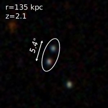
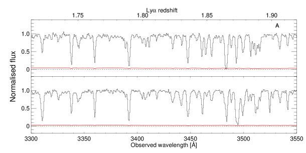
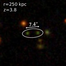
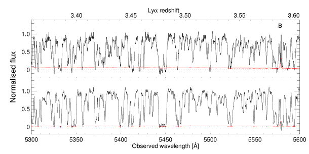
Figure 1: Spectra of the quasar pairs SDSS J073522.43+295710.1, SDSS J073522.55+295705.0 (panel A) and SDSS J102116.98+111227.6, SDSS J102116.47+111227.8 (panel B). The plot shows the continuum normalized flux of the ${\rm Ly\alpha}$ forest as a function of observed wavelength (with the corresponding redshift on the upper axis). The dotted line marks the zero-flux level, while the red solid line shows the amplitude of the $1\sigma$ noise level of each pixel. The two quasar pairs were observed with the Low Resolution Imaging Spectrograph (panel A) and the the echelle spectrograph and imager (panel B) at the Keck telescope. The angular separation between the companions is $5.4^{\prime\prime}$ (panel A) and $7.4^{\prime\prime}$ (panel B), which correspond to an impact parameter of approximately 135 and 250 comoving kpc, respectively. In each pair, the correlation of the absorption features is obvious, implying that the two spectra are probing the same density structures at small scales. Analogous figures for the whole sample are available  (?).

We search for increasing coherence in the ${\rm Ly\alpha}$ forest at progressively smaller quasar pair separations $r_{\perp}\lesssim 300~{}{\rm kpc}$ (angular separation on the sky of $\psi\lesssim 10^{\prime\prime}$) which resolve $\lambda_{P}$  (?). Previously only a handful of high-$z$ quasar pairs with sufficiently small separations were known  (?, ?). We have conducted an observational program to identify close quasar pairs  (?, ?) which makes this measurement possible over the redshift range $1.8<z<3.9$  (?). We used several telescopes to obtain spectra of 25 quasar pairs  (?), with transverse separations ranging from $r_{\perp}=100-500~{}{\rm kpc}$. Fig. 1 shows the overlapping Ly$\alpha$ forests of two quasar pairs in our sample illustrating coherent absorption which results because their separations are comparable to the pressure smoothing scale.

We apply a statistical measure of the ${\rm Ly\alpha}$ forest correlations to this quasar pair data  (?, ?). This technique, based on the phase difference between homologous line-of-sight Fourier modes $k$ of the spectra in the pairs, is maximally sensitive to the pressure smoothing scale $\lambda_{P}$, and minimally sensitive to the temperature-density relation parameters $(T_{0},\gamma)$  (?). The coherence of the Ly$\alpha$ forest is revealed in the statistical distribution of these phase differences $\theta(k,r_{\perp})$, which will tend to be aligned ($\theta\sim 0$) in highly correlated spectra. We split the sample into four redshift bins and measured phase differences for all modes in a resolution-dependent range  (?). Fig. 2 shows the probability distribution function (PDF) of the phase differences (phase angle PDF) for differing values of $k$ and $r_{\perp}$. The fact that the distributions are peaked toward $|\theta|=0$ quantifies the strong correlations which are visible by eye in Fig. 1.

Following  (?), we apply a likelihood formalism for estimating $\lambda_{P}$ from our ensemble of observed phase differences $\Delta\theta(k,r_{\perp})$. For our measurements we adopt a fast flexible semi-numerical model of the IGM based on collisionless dark-matter only N-body simulations, that parametrizes the IGMs thermal state with a temperature-density relation ($T_{0},\gamma$), and pressure smoothing scale $\lambda_{P}$. These thermal parameters are assigned to the dark matter particle distribution in post-processing, and Ly$\alpha$ forest skewers are generated using the fluctuating Gunn-Peterson approximation  (?, ?). This fast simulation method is employed to make our measurements and provides a reference for $\lambda_{P}$ as the smoothing length of the dark matter density field. The $\lambda_{P}$ defined in this way is directly related to the corresponding $\lambda_{P}$ inferred from full hydrodynamical simulations, which we later use to consistently interpret our results  (?).

Imperfections in the data will cause the observed phase angle PDF to depart from the ideal case represented by our model. Specifically, the combination of spectral noise and limited resolution reduces the correlations we are trying to quantify. Metal lines and optically thick Lyman limit systems (LLSs) which are not captured by our simulations provide a stochastic background of absorption which may not be correlated across the two sight lines. To account for these effects, we adopt a forward-modelling approach and implement them into mock Ly$\alpha$ forest spectra for each of the 400 models that we consider  (?). Armed with our likelihood and forward model, we infer the posterior distribution of the thermal parameters using a Markov chain Monte Carlo (MCMC) sampling algorithm  (?). Fig. 3 shows contour plots of the posterior in the thermal parameter ($T_{0},\gamma,\lambda_{P}$) space resulting from this analysis. The horizontal orientation of the contours shows that, as expected from  (?), the phase angle PDF is primarily sensitive to $\lambda_{P}$ and depends only very weakly on $\gamma$ and $T_{0}$. By marginalizing out $\gamma$ and $T_{0}$ we obtain a measurement of $\lambda_{P}$ with statistical errors of $\sim 20-30\%$. We explored the impact of a range of possible systematics related to continuum fitting, imperfect knowledge of the noise and resolution of our spectra, and uncertainties in the abundances of metal lines and LLSs  (?). We conservatively estimate that the combined impact of all these effects increases our uncertainties by at most $\sim 6\%$  (?).

To understand the implications of our $\lambda_{P}$ measurement we compare it to a set of hydrodynamical simulations for several reionization scenarios and resulting thermal histories  (?). This enables a comparison to recent measurements of the IGM temperature based on the thermal Doppler broadening effect along the line-of-sight. The standard picture of IGM thermal evolution is based on the  (?, hereafter HM12) synthesis model of the ultraviolet (UV) background, which provides the photoionization and photoheating rates of IGM gas. In Fig. 4A the HM12 model is compared to recent measurements  (?, ?) of the temperature $T(\Delta_{\star}$) of the IGM at a characteristic density $\Delta_{\star}$, where broad agreement between data and model is observed  (?). Fig. 4B shows that recent measurements of $T_{0}$  (?) require higher temperatures at $z>3$ than the model predicts, and are in apparent disagreement with other measurements  (?). Fig. 4C shows that $\lambda_{P}$ measurements are overall in good agreement with HM12 model predictions.

To study the sensitivity of $\lambda_{P}$ to the IGMs thermal history, we run a hydrodynamical simulation with an abrupt step function reionization history, for which the IGM is cold and neutral until $z_{\rm reion}=7$, after which it experiences the HM12 photoionization and photoheating rates. Whereas in the HM12 model the UV background heats the IGM to $T\sim 10^{4}~{}{\rm K}$ already by $z\sim 15$  (?, ?, ?), reionization heating is delayed until $z\sim 7$ in this late reionization heating model, as illustrated by the red curves in Fig. 4. While its temperature is indistinguishable from the HM12 scenario at all relevant redshifts, this alternative model yields a smaller pressure smoothing scale, illustrating that $\lambda_{P}$ is indeed sensitive to reionization history. The smaller $\lambda_{P}$ values in this model are discrepant at 1.7-$\sigma$ at $z=3$, however the overall statistical disagreement, according to the a-squared test, is only significant at the 55% level. Although the precision on $\lambda_{P}$ achieved with our current quasar pair dataset is not sufficient to rule out either of these models, or set tight constraints on thermal and reionization history, this comparison nevertheless illustrates how pressure smoothing provides additional constraints on thermal models, which are indistinguishable from temperature measurements alone. Finally, we consider a third increased heating model, where the HM12 photoheating rates have been increased by a factor of three  (?) at all redshifts, in an effort to better match the higher temperatures measured by  (?). Fig. 4 shows that this model disagrees with our $z<3$ measurements of $\lambda_{P}$ (as well as with the Becker et al. $T(\Delta_{\star})$ measurements) at the 90% confidence level under a chi-squared test. Our measurement of the pressure smoothing scale appears to favor the lower IGM temperatures measured by  (?, ?), and provides independent confirmation of the standard picture for IGM thermal evolution.

The small-scale structure of IGM baryons could be sensitive to other physics besides the IGMs thermal history. For example, cold dark matter alternatives like warm  (?) or fuzzy  (?) dark matter suppress small-scale fluctuations, whereas primordial magnetic fields have the opposite effect, increasing small-scale power  (?, ?, ?). Other astrophysics such as radiative transfer effects during HeII reionization  (?) or strong feedback from galaxy formation  (?, ?) could also generate additional small-scale fluctuations. Such modifications of either the dark matter or baryons could modify the interpretation of our pressure smoothing scale results. The importance of these effects relative to the standard picture whereby the smoothness of the IGM depends on its thermal evolution driven by cosmic reionization events, can be determined by precisely mapping the statistics of the Ly$\alpha$ forest, from both individual sightlines and quasar pairs, over cosmic time.

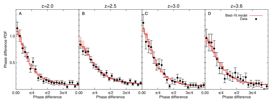
Figure 2: Stacked phase angle PDFs in the four redshift bins. The stacked PDFs are obtained by calculating the phase differences of all pairs in each of the four redshift bins, without separating phases by wavenumber $k$ or transverse pair separation $r_{\perp}$. In this way we condense the entire statistical power of the phase angle data into a single PDF, at the price of mixing together phase angles at different $k$ and $r_{\perp}$, resulting in a loss of spectral and spatial information. This is done to facilitate the visualization of the phase dataset, whereas our actual statistical analysis takes the $k$ and $r_{\perp}$ dependencies into account  (?). The black circles with (Poisson) errorbars are obtained from our data sample, while the red curve represents the thermal model which maximizes the likelihood in our phase analysis, where the models are obtained by post processing a dark-matter only simulation  (?). The red shaded regions delimit the family of models within the 68% confidence level.

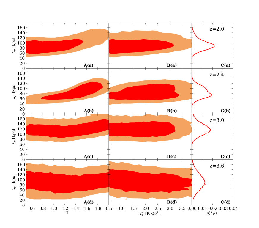
Figure 3: Constraints on the IGM thermal parameters from the phase angle PDF analysis. Panel A: 68% (red) and 95% (light red) confidence levels of the posterior distribution in the $\gamma-\lambda_{P}$ plane. Panel B: same as panel A, but for the $T_{0}-\lambda_{P}$ plane. Panel C: Posterior probability distribution for $\lambda_{P}$ after marginalizing over the other two thermal parameters $T_{0}$ and $\gamma$. The vertical subpanels refer to $z=2,2.4,3,3.6$ (a,b,c and d, respectively). The standard deviation of the distribution of $\lambda_{P}$ for the four redshift bins is $22\%,24\%,19\%$ and $33\%$, respectively. The uncertainty illustrated here do not include the additional $\sim 6\%$ increase in the uncertainties due to systematics  (?).

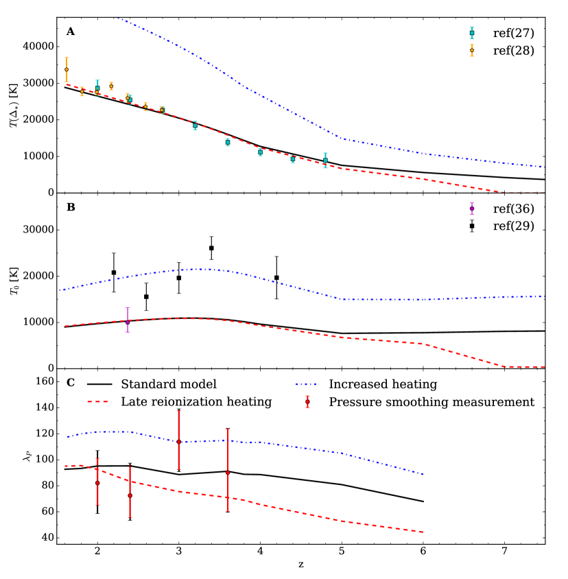
Figure 4: Comparison of our pressure smoothing scale measurement to hydrodynamical simulations. Panel A: The evolution of the temperature $T(\Delta_{\star})$ at the typical density $\Delta_{\star}$ probed by the Ly$\alpha$ forest as defined in  (?). The $T(\Delta_{\star})$ measurements and values of $\Delta_{\star}$ as a function of redshift are taken from  (?, cyan squares) and Boera et al.  (?, orange pentagons). The error bars on these measurements do not include systematic uncertainties caused by lack of knowledge of $\lambda_{P}$ scale (or equivalently the unknown thermal history), and are probably underestimated. Panel B: the temperature at the mean density $T_{0}$ as a function of redshift. The black squares shows measurements from the wavelet analysis of  (?), the magenta circle the results of a Voigt-profile fitting analysis of ${\rm Ly\alpha}$-forest lines from Bolton et al.  (?). In both cases the estimates on $T_{0}$ are fully marginalized over $\gamma$, but again not $\lambda_{P}$, such that uncertainties are also likely underestimated. Panel C: The evolution of the of the pressure smoothing scale as a function of redshift. The red points are the median of the posterior distributions of $\lambda_{P}$ in each redshift bin, while the red errorbars indicate the 16% and 84% percentiles. The black extensions to the errorbars show the small $\sim 6\%$ increase in the uncertainty when systematics are included  (?). The curves in all three panels show predictions from three hydrodynamical simulations  (?). The black lines use the standard heating rates from  (?), for which reionization heating starts at $z=15$. The blue dotted lines show a late reionization heating model for which reionization heating does not occur until $z_{\rm reion}=7$. The blue line is an Increased heating model where we adopt the same reionization redshift $z_{\rm reion}=15$ of the HM12 model, but increase the photoheating rates by a factor of three.

Materials and Methods

1 Overview of the Phase Angle PDF Method

This section provides an overview of the statistical method used to estimate the pressure smoothing scale $\lambda_{P}$ of the IGM. At the end of the section we also specify where the various aspects are described in full detail, so that the reader can effectively use this overview as a brief guide to the rest of supplementary material.

Our technique is based on a statistical analysis of the transmitted flux of the ${\rm Ly\alpha}$ forest in quasar pairs. We define the ${\rm Ly\alpha}$ flux $F$ as the ratio of the observed flux $F_{o}$ to the unabsorbed continuum level $F_{c}$. Following the standard practice, we analyse the flux contrast defined as $\delta F=F/\bar{F}-1$, where $\bar{F}$ is the observed mean flux of the ${\rm Ly\alpha}$ forest at a given redshift. We adopt the value of $\bar{F}$ from the fitting formula of  (?).

We consider the flux contrast in the coeval forest of close quasar pairs. Two ${\rm Ly\alpha}$ forest pixels in different spectra are coeval if they are observed at the same wavelength, implying that the ${\rm Ly\alpha}$ absorption occurred at the same redshift. If two quasars in a pair have a significant fraction of coeval forest and if the two objects are close enough (see below), then the pair can be used to study the transverse correlation of the IGM.

We Fourier-decompose the flux contrast $\delta F(v)$ in the forest of the members of a pair, obtaining the Fourier coefficients $\delta\tilde{F}_{1}(k)$ and $\delta\tilde{F}_{2}(k)$, where the subscripts refer to the two members of each pair. The components are then used to calculate the phase differences $\theta(k)$ of homologous Fourier modes (i.e. with the same wavenumber $k$):

$$\theta(k)=\arccos\left(\frac{\Re[\delta\tilde{F}^{*}_{1}(k)\delta\tilde{F}_{2}(k)]}{\sqrt{|\delta\tilde{F}_{1}(k)|^{2}|\delta\tilde{F}_{2}(k)|^{2}}}\right).$$ (S1)

The alignment of these phases quantifies the coherence of the two spectra and are the fundamental ingredient of our statistical analysis. Note that the normalization factor of the flux contrast (i.e. $\bar{F})$ is divided out in this formula, making phases insensitive to its value. In  (?, hereafter RHW) it is shown that the shape of the statistical distribution of these phase differences is sensitive to the pressure smoothing scale of the IGM. This phase angle probability distribution function (PDF) can be characterized for an ensemble of pairs as a function of the wavenumber $k$ and of the transverse separation $r_{\perp}$. We find that the shape of the phase angle PDF $P_{\rm WC}(\theta)$ can be approximated as a Wrapped-Cauchy (WC) distribution

$$P_{\rm WC}(\theta)=\frac{1}{2\pi}\frac{1-\zeta^{2}}{1+\zeta^{2}-2\zeta\cos\theta},$$ (S2)

which is fully characterized by a single parameter known as the concentration $\zeta$. In the limit where $\zeta\rightarrow 1$, the distribution tends to a Dirac delta function $\delta_{D}(x)$, which is the phase difference distribution of identical spectra. Conversely, $\zeta=0$ results in a uniform distribution, the expected distribution for totally uncorrelated spectra. A negative $\zeta$ gives distributions peaked at $\theta=\pi$ which are non-physical in this context.

In RHW they used a semi-numerical model of the ${\rm Ly\alpha}$ forest based on collisionless dark-matter only simulations to study the dependencies of the phase angle PDF on $[k,r_{\perp}]$, on the smoothing scale $\lambda_{P}$, as well as temperature-density relation of the IGM defined by $T=T_{0}\Delta^{\gamma-1}$. Here $T_{0}$ is the temperature at mean density, $\Delta$ is the density divided by the mean of the Universe and $\gamma$ is the index of the relationship. At a fixed wavenumber $k$, a large separation relative to the pressure smoothing scale results in a flatter distribution of $\theta$, which approaches uniformity for $r_{\perp}\gg\lambda_{P}$ (i.e. incoherent spectra and thus random phases). Conversely, the distribution approaches the fully coherent limit of a Dirac delta function for $r_{\perp}\ll\lambda_{P}$ (almost identical spectra), and the transitions from a strongly peaked distribution to a uniform one occurs when $r_{\perp}$ is comparable to the smoothing scale $\lambda_{P}$. At fixed $r_{\perp}$, lower $k$-modes (i.e. larger scales) are more correlated (smaller $\theta$ values) than high-$k$ modes. This is expected, because sight lines separated by a distance which is small relative to the wavelength of a $k$-mode (i.e. $kr_{\perp}\ll 1$), probe essentially the same density fluctuations associated to the wavenumber $k$. The results of RHW suggested that the phase difference statistic is almost insensitive to the parameters governing the temperature-density relationship $T_{0}$ and $\gamma$, whilst having a strong dependence on $\lambda_{P}$.

By comparing the observed phase differences $\{\theta\}$ in a quasar pair to the predicted phase angle PDFs for a large set of models, we can set constraints on $\lambda_{P}$. To achieve this goal we define a likelihood $\mathscr{L}$ of the ensemble of measured phase differences for a given IGM model, after RHW:

$$\mathscr{L}(\{\theta\}|\lambda_{P},T_{0},\gamma)=\prod_{i}P_{\rm WC}(\theta(k_{i})|\zeta(k_{i},r_{\perp}|\lambda_{P},T_{0},\gamma)),$$ (S3)

which exploits the form of the phase angle PDF defined in eqn. (S2). Here the product is performed over all the modes $k_{i}$ for a given quasar pair with separations $r_{\perp}$. This formalism can be easily generalized to an ensemble of pairs at different separations $r_{\perp}$. The concentration parameter $\zeta$ of the WC distribution is a function of the wavenumber $k$, the separation and the IGM model parameters $\{\lambda_{P},T_{0},\gamma\}$. We generate a grid of thermal models by post-processing a dark-matter only simulation (described in § 5.1), assuming that the IGM is optically thin and in ionization equilibrium, and describing the pressure smoothing with a convolution of the DM particle distribution with a Gaussian kernel. To properly evaluate the likelihood of phases as in eqn. (S3) we need to take into account observational effects like noise and resolution, which may modify the distribution of phases. In addition, we must also consider other astrophysical sources of absorption in the forest like metals and strong H i absorbers. We follow the approach of forward modelling these effects in the simulations, rather than trying to subtract off their effect from the data.

Given a grid of thermal models of the IGM, we can then explore the likelihood in the parameter space to obtain constraints via standard MCMC techniques. To optimize the sampling in parameter space, we used an irregular parameter grid combined with an interpolation scheme based on Gaussian processes. The results of the measurement are tested against a broad range of possible systematic effects, including a potential bias in our estimation of the resolution or the noise, as well as our imprecise knowledge of the number of metal line and strong H i absorbers.

As described below, we run a set of hydrodynamic simulations of the IGM with various assumptions on the thermal and reionization history. We use them to generate mock samples of pairs to which we apply the phase analysis. By comparing the outcome with the results of our measurement we are able to gain insights into the agreement between the current theoretical picture of the IGM and the new constraints from pressure smoothing $\lambda_{P}$ measured from quasar pairs.

The supplementary text is organized as follows: we present the data sample and the selection criteria in § 2, with information on instruments used, resolution, noise level, redshift and angular separation distributions. We then discuss the effect of noise and resolution on the phase distribution, whilst particular care of justifying our assumptions on the full-width at half maximum (FWHM) of the resolution kernels (§ 3). In § 4 we explain how phase differences are calculated from the data, in particular how we address the problem of determining the Fourier coefficients of an irregularly-sampled function. The semi-numerical dark matter simulation models on which we base our phase angle PDF measurement are described in § 5, where we also show how observational effects such as noise, resolution, and contaminants are forward-modelled in the simulations. We then briefly present the statistical tools used in determining the constraints on the pressure smoothing scale (§ 6), in particular the design of the parameter grid, the Gaussian process interpolation, and the MCMC technique. To facilitate the visualization of the sensitivity of this method, we construct plots in § 7, where we stack together phase distributions from different separations and wave numbers in order to reduce the dimensionality of the statistic. In § 8 we quantify the effect of different sources of systematic errors that could impact our analysis. These include continuum fitting uncertainties (§ 8.1), the forward modeling of resolution (§ 8.2), noise (§ 8.3), and of the presence of contaminants (§ 8.4). Finally, in § 9 we explain how we apply the phase analysis to a set of hydrodynamical simulations, allowing the comparison of the transverse coherence in real data to the prediction of realistic IGM models.

2 Experimental Design and the Quasar Pair Dataset

2.1 Quasar Pair Survey

Our goal is to characterize the correlated HI ${\rm Ly\alpha}$ forest absorption in close quasar pairs at $2\lesssim z\lesssim 4$ with separations $<450$ kpc (comoving) corresponding to angular separations $\psi\lesssim 18^{\prime\prime}$ (depending on redshift). As quasar pairs are rare, we have leveraged several large photometric and spectroscopic survey datasets to find the pairs, and then performed dedicated follow-up observations on a number of large telescopes to obtain higher quality data for the ${\rm Ly\alpha}$ forest phase correlation analysis.

The starting point of our experiment is to identify close quasar pairs with angular separations $\psi$ corresponding to comoving separations of $r_{\perp}<450$ kpc (here and in the following, the conversion between angular separation and impact parameter is done assuming the same cosmology specified in § 5.1). To find the pairs, we mine the photometric and spectroscopic databases of the Sloan Digital Sky Survey  (?, SDSS), the Baryonic Oscillation Spectroscopic Survey  (?, BOSS DR12), and the 2dF quasar redshift survey  (?, 2QZ) surveys. Modern spectroscopic surveys bias their selection select against close pairs of quasars to avoid fiber collisions. For the SDSS and BOSS, the finite size of optical fibers precludes discovery of pairs with separation $<55^{\prime\prime}$ and $<62^{\prime\prime}$, corresponding to to 1.37 Mpc and 1.55 Mpc at $z=2$, whereas for the 2QZ survey the fiber collision scale varies from $\sim 30-40^{\prime\prime}$ corresponding to $750-1000$ kpc. In the regions where spectroscopic plates overlap, this fiber collision limit can be circumvented. However, only $\approx 30\%$ of the SDSS spectroscopic footprint and $\approx 40\%$ of the BOSS footprint are in overlap regions. Unfortunately, small separation quasar pairs are rare enough that these overlap regions are not sufficient for building up large samples of quasar pairs close enough for our purposes.

To circumvent this fiber collision limitation, we have conducted a comprehensive spectroscopic survey to discover additional close quasar pairs and to follow-up the best examples for our scientific interests. Close quasar pair candidates are selected from the photometric quasar catalogue of  (?, ?) as well as its recent extension by  (?), and are confirmed via spectroscopy on 4m class telescopes including: the 3.5m telescope at Apache Point Observatory (APO), the Mayall 4m telescope at Kitt Peak National Observatory (KPNO), the Multiple Mirror 6.5m Telescope, and the Calar Alto Observatory (CAHA) 3.5m telescope. Our continuing effort to discover quasar pairs is described in  (?),  (?), and  (?).

Our quasar pair survey has gathered science-grade follow-up optical spectra on large-aperture telescopes using spectrometers with a diverse range of capabilities. This includes data from Keck, Gemini North and South, Magellan, the Large Binocular Telescope (LBT), and the Very Large Telescope (VLT). This large spectroscopic quasar pair data set constitutes the parent sample for the final data set used in this work.

2.2 Spectroscopic Observations

After applying the selection criteria (see § 2.3) for the pressure smoothing scale measurement to our quasar pair spectroscopic database, only spectroscopy from Keck, Magellan, and the VLT contribute to the final sample. We describe each of these observational setups in turn.

At the W.M. Keck Observatory, we have exploited two optical spectrometers to obtain spectra of quasar pairs. One of these was the Low Resolution Imaging Spectrograph  (?, LRIS), which we used to observe 7 of the quasar pairs studied here during a series of observing runs in 2004-2008. We generally used the multi-slit mode with custom designed slit masks that enabled the placement of slits on other known quasars or quasar candidates in the field. LRIS is a double spectrograph with two arms giving simultaneous coverage of the near-UV and red. For our current science goals only the near-UV side (LRIS-B) is relevant, since it covers the ${\rm Ly}\alpha$ forest. We used the D460 dichroic with the $1200$ lines mm^-1 grism blazed at $3400$ Å on the blue side, resulting in wavelength coverage of $\approx 3300-4200$ Å, a dispersion of $0.50$ Å per pixel, and the $1^{\prime\prime}$ slits give a FWHM resolution of about $170{\rm km~{}s^{-1}}$. About half of our LRIS observations were taken after the atmospheric dispersion corrector was installed, which reduced slit-losses in the UV. More information about the observations, data reduction, and a detailed observing log are given in  (?).

At Keck we also used the Echellette Spectrometer and Imager  (?, ESI) to obtain spectra of 10 quasar pairs analysed here. ESI provides continuous spectral coverage from 4000 Å to 10000 Å at a resolution of FWHM = $64{\rm km~{}s^{-1}}$. These data have been previously analyzed for C iv correlations between neighbouring sight lines  (?) and for the analysis of an intriguing triplet of strong absorption systems  (?). Those papers give more information about the data acquisition, reduction, and the observing logs.

Observations for 6 pairs used in this work were obtained with the Magellan Clay telescope using the Magellan Echellette Spectrograph  (?, MagE) during the nights of Universal Time (UT) 2008 January 07-08, UT 2008 April 5-7, and UT 2009 March 22-26. These data cover the wavelength range $\lambda\approx 3050-10300$ Å  and have a FWHM = 62${\rm km~{}s^{-1}}$ or 51 ${\rm km~{}s^{-1}}$, depending on the slit aperture employed. For more more information about the Magellan observations as well the observing logs see  (?).

The XSHOOTER spectrograph  (?) at VLT provided 2 of the pairs of our sample. XSHOOTER’s three arms provide wavelength coverage in the range between 3000 and 25000 Å. One pair (SDSS J000450.90-084452.0, SDSS J000450.66-084449.6 ) has been observed in a program dedicated to this project. The slit aperture used was 0.5”, yielding an estimated resolution of 30${\rm km~{}s^{-1}}$ FWHM. The reduction of the data was performed using a custom data reduction pipeline kindly made available to us by George Becker. Data for one of the pairs used in our analysis (SDSS J091338.97-010704.6, SDSS J091338.30-010708.7) was obtained from the VLT/XSHOOTER archive (program ID:089.A-0855, PI: Finley,H.) and reduced. This slit aperture for these observations was 1.0”resulting in a slightly lower resolution of 69${\rm km~{}s^{-1}}$ FWHM.

2.3 Sample Definition

Here we present the selection criteria that we imposed on our quasar pair spectroscopic database to arrive at the final dataset analyzed in this paper.

We first applied a broad cut to select quasar pairs suitable for the characterizing correlated ${\rm Ly\alpha}$ forest absorption. An obvious prerequisite is the existence of a segment of overlapping ${\rm Ly\alpha}$ forest between the two quasars in the pair, which can be expressed as $(1+z_{\rm fg})\lambda_{\rm{\rm Ly}\alpha}>(1+z_{\rm bg})\lambda_{\rm{\rm Ly}\beta}$. Here $\lambda_{\rm{\rm Ly}\alpha}=1215.67\,{\rm\AA}$ and $\lambda_{\rm{\rm Ly}\beta}=1025.72$ are the rest-frame wavelengths of ${\rm Ly}\alpha$ and ${\rm Ly}\beta$ that define the region of usable ${\rm Ly\alpha}$ forest, and $z_{\rm fg}$ and $z_{\rm bg}$ are the redshifts of the foreground (f/g) and background (b/g) quasar, respectively. To avoid cases where this segment is too small to contribute meaningfully to the statistics, we define the overlapping fraction $f_{\rm ov}$ of the ${\rm Ly\alpha}$ forest as

$$f_{\rm ov}=\frac{(1+z_{\rm fg})\lambda_{{\rm Ly}\alpha}-(1+z_{\rm bg})\lambda_{{\rm Ly}\alpha}}{(1+z_{\rm fg})(\lambda_{{\rm Ly}\alpha}-\lambda_{{\rm Ly}\beta})}$$ (S4)

and we set a lower threshold at $f_{\rm ov}=0.3$, removing in this way projected quasar pairs with large redshift separations.

A second cut is applied to the transverse separation of the pair $r_{\perp}$, evaluated at the redshift of the f/g quasar $z_{\rm fg}$. RHW showed that the most informative pairs are those with impact parameter comparable to the pressure smoothing scale. Existing small-scale measurements of the line-of-sight power spectrum of the ${\rm Ly\alpha}$ forest  (?, ?) exclude pressure smoothing scales larger than $\gtrsim 300-400\,{\rm kpc}$, hence we restrict our analysis to pairs with $r_{\perp}<450\,{\rm kpc}$ (comoving).

Based on the redshift and impact parameter distribution of the data, we decided to divide the data in a set of redshift bins: $1.8-2.2,2.2-2.7,2.7-3.3$ and $3.3-3.9$. The lower limit $z=1.8$ is set to avoid the forest close to the atmospheric cutoff (at $\lambda\sim 3000$ Å), and the bins are wider at higher $z$ to enclose a sufficiently large sample of pairs.

To avoid contamination from the quasar proximity zone we consider only rest-frame wavelengths blueward of $\lambda_{\rm{\rm Ly}\alpha,max}=1190$ Å. Given the particularly large redshift uncertainty $\sim 1000{\rm km~{}s}^{-1}$ of the quasars in our dataset, contamination from Ly$\beta$ absorption is also a concern, and we restrict attention to rest-frame wavelengths redward of $\lambda_{\rm{\rm Ly}\alpha,min}=1040$. The coeval forest in a pair on which we calculate phases is thus defined in the range $\lambda\in[\lambda_{\rm{\rm Ly}\alpha,min}(1+z_{\rm bg}),\lambda_{\rm{\rm Ly}\alpha,max}(1+z_{\rm fg})]$, which is narrower than the one implied by the $f_{\rm ov}$ defined above. The corresponding redshift range is delimited by $z_{\rm min}=\lambda_{\rm{\rm Ly}\alpha,min}/\lambda_{\rm{\rm Ly}\alpha}$ and $z_{\rm max}=\lambda_{\rm{\rm Ly}\alpha,max}/\lambda_{\rm{\rm Ly}\alpha}$.

The set of pairs is then visually inspected in order to find contaminants. Specifically, some quasars exhibit strong associated absorption lines known as Broad Absorption Lines (BAL), which are thought to be produced in the vicinity of the black hole and may reach velocities up to $v\sim 10,000$ km/s. For this reason they could be blueshifted into the ${\rm Ly\alpha}$ forest, causing blending with IGM absorption. Since we are not able to model this blending, we remove from the sample all the pairs in which one of the two spectra is contaminated by BAL.

Strong absorption lines with neutral hydrogen column density $N_{\rm HI}\gtrsim 10^{17}\,{\rm cm^{2}}$, are believed to be associated with galaxies or their circumgalactic media. These so called Lyman Limit systems (LLSs) are a significant source of contamination, since their correlation properties across quasar pair sight lines are determined by the details of galaxy formation, rather than by the simpler low-density hydrodynamics governing the ${\rm Ly}\alpha$ forest. Standard practice in studies of ${\rm Ly}\alpha$ forest statistics is to mask out these LLS, forward model them, or some combination of these approaches  (?). The strategy we adopt here is to identify and mask all objects for which we can clearly see damping wings in the spectrum, which corresponds approximately to a column density threshold of $N_{\rm HI}\gtrsim 10^{19}{\rm cm}^{-2}$, which encompasses Damped Lyman-$\alpha$ systems (DLAs) ($N_{\rm HI}>10^{20.3}{\rm cm}^{-2}$) as well as so called super-LLSs ($10^{19}\,{\rm cm}^{-2}<N_{\rm HI}<10^{20.3}{\rm cm}^{-2}$). As our algorithm for measuring phase angles requires contiguous spectral coverage, when strong absorbers are present, we simply split the unmasked data into multiple segments specified by redefining $z_{\rm min}$ and $z_{\rm max}$ for each of them. Column densities in the range $10^{17}\,{\rm cm}^{-2}<N_{\rm HI}<10^{19}{\rm cm}^{-2}$ cannot be reliably identified in spectra of our wavelength coverage, ${\rm S/N}$ ratio, and resolution, so rather than masking, we directly forward model such absorbers by adding them to our models. In § 5.3 we discuss the details of this procedure, and the impact of these strong absorbers on our results in detail.

At the end of this process we obtain a list of paired wavelength regions of coeval ${\rm Ly\alpha}$ forest, delimited by $z_{\rm min}$ and $z_{\rm max}$. Each quasar pair may have more than a single segment. For each of these segments, we evaluate the signal-to-noise ratio per observed frame Angstrom ${\rm S}/{\rm N}_{\rm 1\AA}$ in the two spectra, between $z_{\rm min}$ and $z_{\rm max}$. We only include in the final sample those pairs for which both members of the pair have ${\rm S}/{\rm N}_{\rm 1\AA}>10$. To determine ${\rm S}/{\rm N}_{\rm 1\AA}$, we first compute the median signal-to-noise ratio per pixel ${\rm S}/{\rm N}_{\rm px}$ of the spectrum over the interval $[(1+z_{\rm min}),(1+z_{\rm max})]\lambda_{\rm{\rm Ly}\alpha}$. We then multiply ${\rm S}/{\rm N}_{\rm px}$ by the factor $\sqrt{1\,{\rm\AA}/\Delta\lambda_{\rm px}}$ to put the different spectral resolution data utilized in this study onto a common scale, where $\Delta\lambda_{\rm px}$ is the median pixel width in each spectrum.

The vast majority of the quasar pairs identified by our survey are binaries with small redshift separations, or projected quasar pairs at different redshifts. At the angular separations we consider $\sim 4-10^{\prime\prime}$, only a small fraction of quasar pairs at the same redshift are expected to be gravitational lenses, i.e. a double image of the same source, owing to the relative paucity of such wide-separation lenses  (?). We nevertheless conducted a literature search for all quasar pairs selected by the criteria above and found two which were known to be gravitational lenses. Of the remaining quasar pairs, none have spectra of sufficient similarity to warrant the lensing hypothesis, nor did any show evidence for a lens galaxy in the SDSS imaging (for such wide separation lensed quasars, the lens is often visible as a group of galaxies even in the relatively shallow SDSS imaging). In principle, lenses can also be used to study the coherence of the IGM if the lens redshift is precisely known, in which case the dependence of the impact parameter with redshift can be easily modelled. However, lenses typically probe small impact parameters at ${\rm Ly\alpha}$ forest redshifts of $100\,{\rm pc}-10\,{\rm kpc}$  (?). The smallest separations are likely insensitive to the pressure smoothing scale, whereas even for larger $\sim 10\,{\rm kpc}$ separations, the analysis is likely much more sensitive to incoherence caused by LLSs and/or metal line absorbers (see § 5.3) which would require a much more careful treatment and modeling procedure. For this reason, we discard the pairs identified as gravitational lenses.

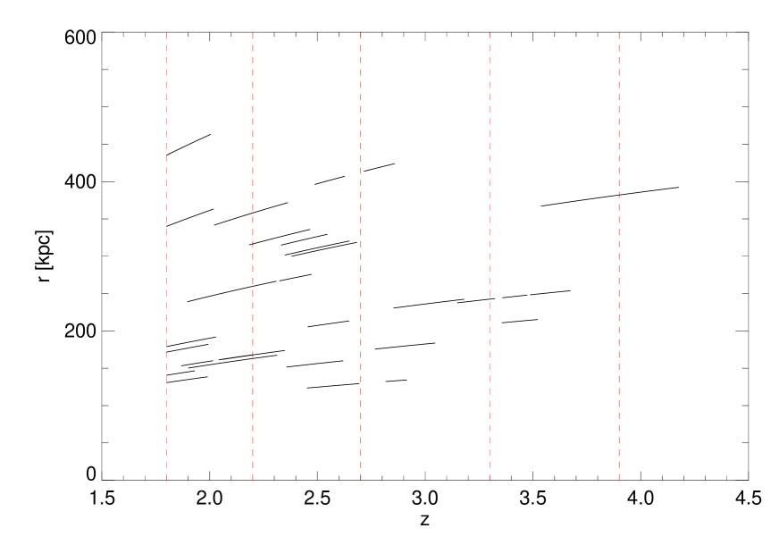
Figure S1: The distribution of our sample in redshift $z$ and in transverse separation $r_{\perp}$. Each black line represents a segment of overlapping ${\rm Ly\alpha}$ forest in a pair. The length of a segment depends on the redshift difference between the two quasars and on the presence of DLAs or other contaminants that require excluding part of the forest. The atmospheric cutoff sets a lower limit for all pairs at $z\approx 1.7$. The lines are curved because the impact parameter evolves with redshift converging toward us. The vertical red dotted lines delimit the four redshift intervals to which we split the sample.

The final sample obtained from our selection criteria is illustrated in Fig. S1. The lines trace the coeval ${\rm Ly\alpha}$ forest in the pairs, following the evolution of the impact parameter as a function of redshift. The extent of the overlapping segments depends on the respective redshifts of the quasar in the pair (see eqn. (S4)), as well as on our masking of strong absorbers, which appear as gaps in the lines. A complete list of the coeval ${\rm Ly\alpha}$-forest segments is provided in Table LABEL:tab:sample, together with all the relevant parameters for each pair. The redshift binning determines a further split of the sample, as a result of intersection of each of the segments with the four $z$ bins. All intersections that span a redshift interval smaller than $\Delta z=0.08$ are discarded.

2.4 Continuum Fitting and Data Preparation

We fitted the continuum manually using a fitting algorithm that performs a cubic spline interpolation between manually inserted break points, resulting in a continuum tracing the undulations and emission features of the quasars which are obvious to the reader. These features, of course, are more easily discerned in the higher ${\rm S/N}$ spectra. This led, in part, to the imposed S/N criterion of our sample. At the typical spectral resolution of our data, one generally expects the normalized flux to lie below unity (in the absence of noise) owing to integrated ${\rm Ly\alpha}$ opacity from the IGM. We took this into full consideration when generating the spline continuum and also allowed for the expected increase in ${\rm Ly\alpha}$ opacity with increasing redshift. We emphasize that phase correlation statistic that we employ to measure the pressure smoothing scale is not particularly sensitive to errors in the continuum-placement, as we explicitly demonstrate in § 8.

Since our analysis involves a statistic computed in velocity space, we transform the wavelengths into velocities according to

$$\Delta v=c\log(\lambda/\lambda_{0}),$$ (S5)

where $c$ denotes the speed of light, $\Delta v$ is the relative velocity between two points responsible for resonant ${\rm Ly\alpha}$ absorption at observed wavelengths $\lambda$ and $\lambda_{0}$. Here $\lambda_{0}$ is an arbitrary reference wavelength, typically the lowest in a segment, taken as the origin of the velocity space. For matter moving with the Hubble flow, this velocity $\Delta v$ corresponds to a comoving distance of

$$\Delta x=\frac{(1+z)\Delta v}{H(z)}.$$ (S6)

where the $H(z)$ is the Hubble parameter at the observed redshift, which is calculated assuming the same cosmology specified in § 5.1.

3 Noise and Resolution

The distribution of phases may deviate from its intrinsic shape determined by IGM physics, depending on the level of noise and the spectral resolution of the observations. Specifically, noise results in scatter of the Fourier components into which we decompose the spectra, randomly changing both their moduli and their phases. Since phases are scattered independently in the two spectra of a quasar pair, noise will broaden the phase difference PDF. The broadening will be more evident in the high-$k$ modes, which are damped by the resolution cut-off and whose signal is therefore dominated by the noise. These considerations call attention to the estimates of the noise and resolution of our spectra, which are necessary inputs to our forward modelling procedure, which will be described in § 5.

The data reduction pipelines used to reduce the data deliver accurate estimates for the noise, which takes into account the distinct contributions from photon counting noise from both the sky background and the object, as well as detector readout noise. The accuracy of the algorithms used to estimate the spectral noise in our data reduction pipelines were recently characterized in  (?), where it was found that the pipeline delivers noise estimates that are accurate to $\lesssim 10\%$.

The resolution is a more delicate issue. For slit spectroscopy, the width of calibration spectral lines provided by an arc lamp, taken during daytime, can be used to determine the resolving power of the spectrometer for a source (i.e. the arc lamps) which uniformly illuminates the spectrograph slit. We refer to this resolution measured from arc lines as the slit resolution of the spectrometer. For Keck/LRIS we directly measure this resolution from the FWHM of arc-lines, whereas for echelle spectrometer Keck/ESI, Magellan/MagE, and VLT/XSHOOTER we adopt the slit resolution reported in the instrument manuals (also based on arc-line widths) for the order in question and the slit used. These values of the slit resolution are listed as the FWHM in Table LABEL:tab:sample.

However, the true resolution of a spectrum of a point source will depend on the seeing during the observation, and could be significantly smaller than the slit resolution if the data is obtained in good seeing conditions. For these reason we expect the value of the FWHM listed in Table LABEL:tab:sample to typically overestimate the true resolution of the spectra.

To assess the accuracy of these resolution estimates we compute the line-of-sight power spectrum of the flux contrast $\delta F$ and compare it with a measurement from a distinct high-resolution quasar sample. The idea behind this test is that smearing of the spectra due to the resolution of the spectrograph modifies the flux power spectrum in a known way. Given an estimate for the resolution, we can undo the effect of this smearing in our data, and compare our resulting resolution-corrected power spectrum to the power spectrum of the ${\rm Ly\alpha}$ forest from an independent fully resolved dataset. If, as we suspect, the slit resolution FWHM is larger than that of our actual data, this will be manifest as a mismatch between these two power spectra, and we can correspondingly adjust our resolution estimate to the value that produces the best match. In addition to calibrating our spectral resolution, this comparison provides a basic sanity check on the various steps of the procedure (data reduction, noise estimates, continuum normalization, masking strong absorbers) required to generate the $\delta F$ fields from our spectra.

We consider a sample of quasars composed of 38 spectra observed with the Ultraviolet and Visual Echelle Spectrograph  (?, UVES) and 37 spectra from the Keck Observatory Database of Ionized Absorption  (?, KODIAQ) project observed with the High Resolution Echelle Spectrometer  (?, HIRES). We select objects with S/N $>20$ per 6 km/s interval inside the usable ${\rm Ly\alpha}$ interval. The resolution of the sample is 6${\rm km~{}s^{-1}}$ FWHM, except some of the HIRES spectra which have FWHM of 3${\rm km~{}s^{-1}}$. The sample covers the redshift range between $z=1.7$ and $z=3.5$.

Similar to our approach, DLAs are identified in the high-resolution data through their damping wings and masked. Metals absorbers are identified redwards of the ${\rm Ly\alpha}$ line by looking for doublets lines for common transitions (Si iv, C iv, Mg ii, Al iii, Fe ii). We then mask spectral regions of the ${\rm Ly\alpha}$ forest where we expect other lines originating from these absorbers for different possible metal transitions (removing 60${\rm km~{}s^{-1}}$ around the central redshift).

In order to calculate the flux power spectrum of both the quasar pair data and the high-resolution data, we follow the approach of  (?), which we summarize here. The flux contrast $\delta=F/\bar{F}-1$ is considered to be the sum of the contribution of the forest and noise: $\delta=\delta_{F}+\delta_{n}$. Under the assumption that the Fourier modes of the two components are uncorrelated, we can decompose the total power as the sum of the noise power and of the forest power. The latter can therefore be calculated as

$$P_{\rm 1D}(k)=\frac{P^{\rm raw}(k)-P^{\rm noise}(k)}{W^{2}(k,\sigma_{R},\Delta v)}$$ (S7)

where $P^{\rm raw}(k)$ is the power spectrum of the observed spectrum and $P^{\rm noise}(k)$ is the power spectrum of the noise estimated from the pipeline. $W$ is a filtering function which models the response of the spectrograph, and depends on the wave number $k$, on the resolution width $\sigma_{R}$ and on the pixel scale $\Delta v$ in the following way

$$W(k)=\exp\left(-\frac{(k\sigma_{R})^{2}}{2}\right)\times\frac{\sin(k\Delta v/2)}{k\Delta v/2}.$$ (S8)

The only relevant difference between our approach and the method of  (?) is that our spectra do not have a regular binning in velocity space, therefore we need to use the Lomb-Scargle periodogram to compute the power, along the lines of the technique described in § 4.1.

When calculating the flux power spectrum of the quasar pair sample we divide the data into the three lower redshift bins used in the phase analysis, i.e. $\Delta z=1.8-2.2,2.2-2.7,2.7-3.3$ (called “coarse” bins in the rest of this section). We ignore the highest-redshift bin for this study, because of the small number of quasar pairs in this bin and the fact that our high-resolution dataset does not extend beyond $z=3.5$, precluding a meaningful comparison. We will thus assume that the results we obtain about the resolution can nevertheless be extended beyond $z=3.3$. The power spectrum is first calculated separately on the segments of ${\rm Ly\alpha}$ forest we defined in § 2.3, and subsequently averaged in logarithmic bins in $k$ and over all segments. Uncertainties are calculated by bootstrapping over these segments. Since the forest of quasar pairs is correlated, we are probably underestimating the errors in this way. However, the aim of this section is not to do a rigorous statistical analysis but only to verify the approximate agreement of the power spectrum of the pair sample with high resolution data.

When calculating the power spectrum of the UVES and HIRES sample we initially adopt redshift bins spaced by $\Delta z=0.2$ between $z=1.7$ and $z=3.5$. We will refer to these small intervals as $\Delta_{j,\rm HR}z$, identified by the index $j$, to distinguish them from the redshift bins relative to the pair analysis. The power and the relative errors are then obtained in the same way as for the quasar pair data. However, the redshift bins in which the quasar pair data are subdivided are coarser, and the pairs path length distribution is not uniform across these bins. Since the power level evolves with redshift, we need to take into account the redshift distribution of the forest path length in coarse bins when comparing the quasar pair power spectrum to the high-resolution data. To do this, we start from the high-resolution power in the $\Delta_{j,\rm HR}z=0.2$ bin, and we then use a weighted average to calculate the corresponding power in the coarser redshift intervals in which the pair sample is binned. The weights depend on the path length of the forest in pairs within each $\Delta_{j,\rm HR}z$ bin. More precisely we define

$$w_{j}=\frac{\sum_{i}|\Delta_{i}z\cap\Delta_{j,\rm HR}z|}{\sum_{i}|\Delta_{i}z|},$$ (S9)

where $\Delta_{i}z$ is the redshift interval spanned by the $i$th segment of the pair sample in the considered coarse redshift bin and the sum is performed over all the segments in the coarse bin. Note that the denominator is equal to the total path length of the ${\rm Ly\alpha}$ forest in the quasar pairs sample for the said bin. The power from the high resolution sample is therefore computed as

$$P_{\rm coarse}(k)=\sum_{j}P_{j,\rm HR}(k)w_{j}$$ (S10)

where $P_{j,\rm HR}$ is the power spectrum of the high-resolution data in the $\Delta_{j,\rm HR}z$ redshift interval. This is repeated for each coarse bin.

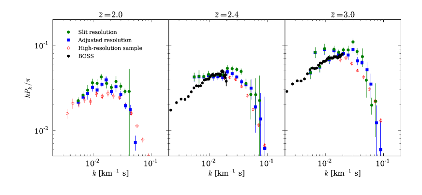
Figure S2: Test of the resolution modeling using the power spectrum of the ${\rm Ly\alpha}$ flux contrast in three redshift bins. The noise power has been subtracted and a Gaussian resolution correction has been applied, as described in the text. The red open pentagons are calculated from a sample of high-resolution spectra observed with UVES and HIRES, and are used as a benchmark for the comparison with our data. The green circles mark the power spectrum of the ${\rm Ly\alpha}$ forest in our pair sample, assuming the nominal resolution of the instrument, whereas for the blue squares we increased our assumed resolution by 20% . Uncertainties are estimated via a bootstrap technique, but they are likely to be underestimated because the spectra are not all statistically independent, as there is correlation of the ${\rm Ly\alpha}$ forest power between the members of each pair. Where possible, we use published measurements of the power spectrum  (?) to verify the consistency of our calculation at low-$k$ (black circles). The power spectrum calculated from the pair sample is overall noisier, as expected, than the high-resolution one. We find that assuming the nominal resolution of the instrument overestimates the signal, indicating that the resolution is typically underestimated. A correction of $20\%$ to the resolution FWHM estimates accommodates the discrepancy between the power at an acceptable level, and is taken as our standard assumption in the forward-modelling procedure.

The results are shown in Fig. S2, together with literature values of the power calculated from the BOSS sample  (?). The BOSS power spectrum was measured in the same $\Delta_{j,\rm HR}z$ bins as our high-resolution data, so we applied the same weighted average described above to produce this figure. The BOSS dataset only samples redshift $z>2.1$, for which reason we could not calculate the relative power in the lowest-redshift coarse bin. The power spectrum calculated from our pair sample is in broad agreement with the power from high-resolution data, but has a clear excess at the high-$k$ end. We attribute this discrepancy to an underestimation of the resolution, following the argument presented above. In fact, if the resolution is underestimated, the filtering correction to the power in eqn. S8 would overcompensate for the resolution cut at high-$k$, adding spurious power.

We choose to apply a correction factor to all of our resolution estimates in order to improve the match of the power spectra. By visual inspection, we find that if we decrease the FWHM of all our pairs by 20%, the agreement between the quasar pair and high-resolution power spectra is better (Fig. S2). This correction defines our default value for the resolution assumed throughout the text. The choice of the correction factor is not made via a rigorous statistical analysis, and is somewhat arbitrary. Furthermore, we are adopting a fixed factor for all data, while each pair has been observed under particular conditions and using a specific slit width. These simplifications are ultimately justified by the weak sensitivity of phase differences to resolution, as we show in a consistency test a posteriori (see § 8.2).

4 Phase Calculation on Pair Spectra

Our method relies on the calculation of phase differences of Fourier components. However, Fourier transforming the the ${\rm Ly\alpha}$ forest of real observed spectra requires further elaboration. While in simulations we generate mock spectra on perfectly regular grids in velocity space, the pixels of observed spectra are in most of the cases unevenly spaced. Since the discrete Fourier transformation is defined for evenly-sampled functions, we have to either interpolate or rebin the data onto a regular grid, or to use approximate methods without modifying the sampling. The two methodologies have opposite advantages and disadvantages, so we decide to implement both and to check that they lead to consistent results (§ 4.3). This test will also demonstrate that our results are not affected by pixel rebinning at the data-reduction level.

4.1 Method 1: Least-Square Spectral Analysis

A widely-used approach to generalize Fourier transformation to irregularly-sampled series is the so called least-square spectral analysis (LSSA). It consists of fitting a function $f(x_{i})$ with a linear combinations of trigonometric functions $\cos(k_{j}x_{i})$ and $\sin(k_{j}x_{i})$, where $\{x_{i}\}$ is the set of points where $f$ is sampled and $\{k_{j}\}$ are the wave numbers of the modes that we want to fit. This leads for example to the Lomb-Scargle periodogram  (?), a method often employed to calculate the power spectrum of a signal. It is also possible to follow this strategy to recover the phase information, which is what we want to calculate in quasar spectra. We follow for this purpose the method described in  (?) which we briefly summarize here.

The Fourier decomposition is given by the minimization, for each different $k_{j}$ of

$$||f({\bf x})-c_{j}\cos(k_{j}{\bf x})+s_{j}\sin(k_{j}{\bf x})||$$ (S11)

where in our case $\bf{x}$ is the array of the velocity-space pixels in a spectrum, $f$ is the transmitted flux of the ${\rm Ly\alpha}$ forest, $||g({\bf x})||=\sum_{i}g^{2}(x_{i})$ denotes the squared norm and $(c_{j}s_{j})$ are the coefficients that we need to determine. Put another way, we want to find the projection of $f$ on the functional subspace defined by the linear combinations of $\cos(k_{j}{\bf x})$ and $\sin(k_{j}{\bf x})$. In the case where $x_{i}$ are evenly spaced and $k_{j}=2\pi j/L$, with $L$ being the total length of the spectrum, this is equivalent to the standard Fourier decomposition. For generic $\{x_{i}\}$ and $\{k_{j}\}$ the linear subspaces relative to different $k$ may not be orthogonal and may not form a complete functional basis, so this fitting procedure cannot be properly regarded as a decomposition.

The minimization of eqn. S11 is obtained via the Moore-Penrose pseudo-inverse matrix  (?) applied to the linear system

$$f({\bf x})=(c_{j}\ s_{j})\Omega_{j}$$ (S12)

where $\Omega_{j}$ is defined as

$$\Omega_{j}=\left(\begin{array}[]{ccc}\cos(k_{j}x_{1})&...&\cos(k_{j}x_{n})\\ \sin(k_{j}x_{1})&...&\sin(k_{j}x_{n})\\ \end{array}\right).$$ (S13)

The pseudo inverse is then $\Omega_{j}^{+}=\Omega_{j}^{T}(\Omega_{j}\Omega_{j}^{T})^{-1}$ and the coefficients are estimated by

$$(c_{j}\ s_{j})=f({\bf x})\Omega_{j}^{+}.$$ (S14)

According to the pseudo-inverse properties, these coefficients are exactly the ones that minimizes $||f({\bf x})-(c_{j}\ s_{j})\Omega_{j}||$, i.e. eqn. S11. When the system has a solution this norm is zero, but for our problem this is never the case. This definition of the pseudo-inverse requires that $\Omega_{j}\Omega_{j}^{T}$ is invertible, which is however always satisfied for reasonable pixel distributions.

By explicitly writing eqn. S14 we obtain

$$(c_{j}\ s_{j})=\left(\begin{array}[]{c}\sum_{i}f(x_{i})\cos(k_{j}x_{i})\\ \sum_{i}f(x_{i})\sin(k_{j}x_{i})\\ \end{array}\right)^{T}\left(\begin{array}[]{cc}\sum_{i}\cos^{2}(k_{j}x_{i})&\sum_{i}\cos(k_{j}x_{i})\sin(k_{j}x_{i})\\ \sum_{i}\cos(k_{j}x_{i})\sin(k_{j}x_{i})&\sum_{i}\sin^{2}(k_{j}x_{i})\end{array}\right)^{-1}$$ (S15)

where the diagonal terms are non-zero because $\sin(k_{j}\bf{x})$ and $\cos(k_{j}\bf{x})$ are not orthogonal in general. Nevertheless it is possible to apply a phase shift to the coordinates such that, for a given $k_{j}$, the non diagonal terms vanish  (?). It can be shown that the shift is equal to

$$T_{j}=\frac{1}{2k}\arctan\frac{\sum_{i}\sin(k_{j}x_{i})}{\sum_{i}\cos(k_{j}x_{i})}.$$ (S16)

After diagonalization, the equation above simplifies to

$$(c_{j}\ s_{j})=\left(\frac{\sum_{i}f(x_{i})\cos(k_{j}(x_{i}-T_{j}))}{\sum_{i}\cos^{2}(k_{j}(x_{i}-T_{j}))}\ \ \frac{\sum_{i}f(x_{i})\sin(k_{j}(x_{i}-T_{j}))}{\sum_{i}\sin^{2}(k_{j}(x_{i}-T_{j}))}\right),$$ (S17)

which is the expression we are looking for. The power spectrum immediately follows from this result as $P(k_{j})=c_{j}^{2}+s_{j}^{2}$.

If we need to recover phase information we must consider that phases are changed by the Lomb shift, therefore we have to apply the inverse translation at each $k$. This is easily done by defining the Fourier coefficients in the complex representation as

$$F(k_{j})=(c_{j}+is_{j})e^{ik_{j}T_{j}}.$$ (S18)

We are now ready to calculate phase differences in the usual way

$$\theta(k)=\arccos\left(\frac{\Re[\tilde{F}_{1}^{*}(k)\tilde{F}_{2}(k)]}{|\tilde{F}_{1}(k)||\tilde{F}_{2}(k)|}\right)$$ (S19)

where $F_{1}$ and $F_{2}$ are the transmitted fluxes of the ${\rm Ly\alpha}$ forest in the two spectra of the pair.

A final caveat concerns non-orthogonality: the Fourier components do not form an orthogonal basis if the pixel spacing is irregular. For this reason, the cross products $C_{l,m}=\sum_{i}\exp(-i(k_{m}-k_{l})x_{i})$ could be different from zero, therefore inducing a systematic correlation between the Fourier coefficients and potentially a correlation between phase differences. We anticipate that this effect should be important only at scales comparable to the pixel separation, however we force the orthogonality of the components in the following way: after calculating the coefficient $\tilde{F}(k_{0})$ we subtract the corresponding component from the original function by defining

$$F^{\prime}({\bf x})=F({\bf x})-\tilde{F}(k_{0})e^{-ik_{0}{\bf x}}.$$ (S20)

Then we calculate the next coefficient $\tilde{F}(k_{1})$ on the residual function $F^{\prime}({\bf x})$. We iterate this procedure until all the coefficients are calculated. This algorithm is a standard orthogonalization process, and requires specifying the order on which the components are subtracted. The most natural choice for us is starting with the large scale modes, i.e. with the lowest wavenumber, which are the least affected by noise and resolution. This procedure cannot obviously remove intrinsic correlations between different Fourier modes originated from cosmological or physical processes. However it was shown in RHW that these are negligible in the relevant range of wavenumbers.

4.2 Method 2: Rebinning on a Regular Grid

A second possibility is to rebin the observed flux pixels onto a regular grid, to allow the standard calculation of the Fourier coefficients. The advantage of this method is that we avoid approximations deriving from the least-square evaluation of the phases, but on the other hand, we do not have a clear picture of how the rebinning modifies the Fourier phases. The pros and cons of this approach are complementary to the LSSA procedure described in the previous section, therefore we decide to adopt both of them and check that the results are consistent, assuring in this way that our approximate calculation of phases is not a source of bias (§ 4.3).

In order to consistently calculate phase differences, not only is it necessary to bin the pixels of each spectrum onto a regular grid in velocity space, but also to use the same regular grid for both spectra of the pair. We define the common regular grid from the original arrays via a simple procedure. For a single spectrum with $N$ irregular pixels located at $\{v^{0}_{i}\}$, the step of the regularized array is $\Delta v=(v^{0}_{N}-v^{0}_{1})/(N-1)$ and the full vector $\{v_{i}=v^{0}_{1}+i\Delta v\,\forall i=0..N\}$. When considering two spectra with different pixels arrays $\{u^{0}_{i}\}$ and $\{w^{0}_{i}\}$, having respectively $N$ and $M$ points, we define the grid in the common velocity interval $I=[\max(u^{0}_{1},w^{0}_{1}),\min(u^{0}_{N},w^{0}_{M})]$. We then count the number of pixels encompassed within this interval for each of the two spectra, and we take the smallest of the two numbers to be the cardinality of the common grid grid $N_{g}$. In this way we avoid oversampling in the rare cases where one spectra is observed with a finer pixel scale than the other. The spacing is then simply $|I|/(N_{g}-1)$, where $|I|$ is the total length of the interval. We finally rebin the transmitted fluxes onto the newly-defined pixel vector and we are set to compute the phase differences by standard Fourier analysis.

4.3 Methods Comparison

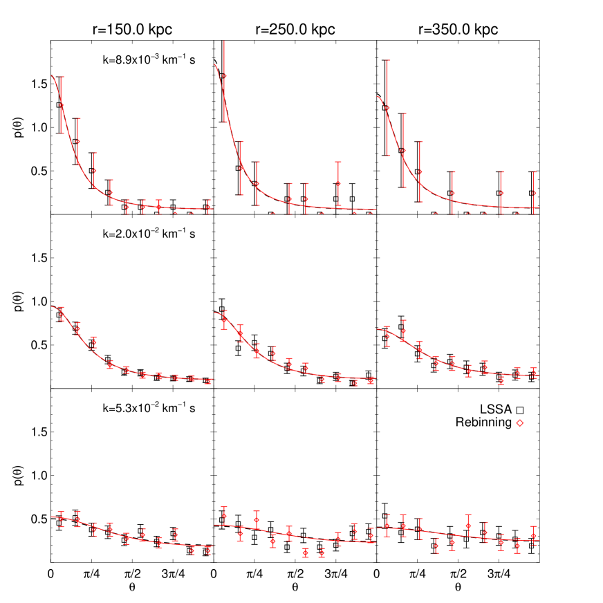
Figure S3: Comparison of the two phase calculation methods applied to data at $z=2$: least square spectral analysis (black squares) and rebinning on a regular grid to apply Fourier transformation (red diamonds). The best-fitting wrapped-Cauchy functions are shown as solid lines, with the same colors. The distributions are derived by first calculating all the phase differences in the sample of pairs within the redshift range $z\in 1.8-2.2$, then subdividing them in nine sets according to the transverse separation $r_{\perp}$ and the wavenumber $k$, as described in the text. The two methods agree well in all cases, and the wrapped-Cauchy fits are close to each other, implying that the phase distributions are statistically equivalent. This demonstrates the robustness of the approximated method that we use to calculate phases.

We have presented two possible ways of calculating phases of irregularly sampled functions: one employs least-square spectral analysis (LSSA), the other rebins the function onto a regular grid and applies the standard discrete Fourier transform. Since the two methods imply complementary approximations, checking that they lead to consistent phase distributions is a good test of the accuracy of these calculations. In Fig. S3 we show the distributions of the observed phases binned in $k$ and $r_{\perp}$, adopting both methods. This figure is constructed by calculating the phases of all the segments in the redshift bin $z\in 1.8-2.2$, without restriction on $k$ and $r_{\perp}$. Subsequently we group the phases according to the wavenumber and separation, by subdividing the $k$-space in three bins ($0.008-0.01$ km^-1 s, $0.01-0.04$ km^-1 s and $0.04-0.07$ km^-1 s) and the $r_{\perp}$-space in the intervals $100-200$ kpc, $200-300$ kpc, and $300-400$ kpc. The phase PDF of each of the nine subgroups is shown in the nine panels in Fig. S3. We choose to do this test at low redshift because the data resolution is typically lower and the pixel sampling coarser, therefore it should be easier to highlight problems in the phase calculation on an irregularly-sampled velocity grid.

In all cases the two methods agree well, and most importantly the statistical estimator that we use in the likelihood, i.e. the wrapped-Cauchy concentration parameters, are practically identical. This can be seen by fitting the wrapped-Cauchy function to the two distribution, which are indistinguishable at all $r_{\perp}$ and $k$ (Fig. S3). We also emphasize that the approximate Fourier transformation is also part of the forward-modelling of simulations (see § 5.5), so even in the case of a significant effect on phase distributions, it would be taken into account in our calibration. From now on the standard method adopted to calculate phase differences, both in data and simulations, is the LSSA technique.

5 Forward Modeling the Phase Angle PDF

To connect the observed phase differences in quasar pairs with the quantity we want to measure, the pressure smoothing scale, we run a grid of semi-numerical models based on a dark-matter simulation. We adopt an approximate scheme that enables a detailed exploration of IGM thermal parameter space, defined by the pressure smoothing scale $\lambda_{P}$, the temperature at the mean density $T_{0}$, and the slope of the temperature-density relationship $\gamma$.

A proper comparison of data to models requires that we account for aspects of the data which are not present in our idealized models, such as noise, resolution, and the presence of contaminants such as metal lines and strong HI absorption systems. Since it is not straightforward to subtract these effects from distribution of phase angles, we adopt a forward-modeling approach, which involves producing models with the same properties as our data. In this way the analysis of phase angles is calibrated against the simulations in a consistent way. Briefly speaking, the calibration is obtained by creating, for each observed pair, an entire ensemble of simulated copies, with the same transverse separation, the same noise amplitude and the same resolution, but varying the underlying IGM properties that we want to study.

In this section we summarize our IGM model and we describe each step of the forward-modeling procedure.

5.1 Dark-Matter Simulations and Parameter Grid

Ideally, we would like to explore a large set of thermal models of the IGM. However, because the pressure smoothing scale $\lambda_{P}$ is sensitive to the entire thermal history, the dynamic range we would need to span is not easily achievable with current hydrodynamical simulations of cosmological volumes. Therefore we opt for a fast, approximate method based on N-body simulations, which enables to easily cover the relevant space of IGM parameters. In § 9 we will use a set of hydrodynamical simulations as a reference to compare our results with the prediction of more accurate models.

We base our model of the Ly$\alpha$ forest on a N-body dark matter (DM) only simulation. In this scheme, the simulation provides the dark matter density and velocity fields  (?, ?), and the gas density and temperature are computed using simple scaling relations motivated by the results of full hydrodynamical simulations  (?, ?, ?). We do not consider the effect of uncertainties on the cosmological parameters, as they are constrained by various large-scale structure and CMB measurements to much higher precision than the thermal parameters governing the IGM.

We used an updated version version of the TreePM code  (?) to evolve $2048^{3}$ equal mass ($2.5\times 10^{5}\,h^{-1}M_{\odot}$) particles in a periodic cube of side length $L_{\rm box}=30\,h^{-1}$Mpc with a Plummer equivalent smoothing of $1.2\,h^{-1}$kpc. The initial conditions were generated by displacing particles from a regular grid using second order Lagrangian perturbation theory at $z=150$. This TreePM code has been compared to a number of other codes and has been shown to perform well for such simulations  (?). Recently the code has been modified to use a hybrid Message Passage Interface (MPI) + Open Multi-Processing (OpenMP) approach which is particularly efficient for current supercomputers. We also adopt the cosmological parameter from  (?), i.e. density parameters for the cosmological constant of $\Omega_{\Lambda}=0.68$, for the matter of $\Omega_{m}=0.32$ and reduced Hubble constant $h=0.67$. We focus on four snapshot at $z=2,2.4,3,3.6$, approximately at the center of the redshift intervals in which we bin the data.

The baryon density field is obtained by smoothing the dark matter distribution; this mimics the effect of the pressure smoothing (see  (?) for a discussion about this kind of approximations). For any given thermal model, we adopt a constant pressure smoothing scale $\lambda_{P}$, rather than computing it as a function of the temperature, and this value is allowed to vary as a free parameter (see below). The dark matter distribution is convolved with a window function $W_{\rm IGM}$ in real space. By the convolution theorem, this operation is equivalent to multiplying the Fourier components of the density field by the Fourier-transform of the window function

$$\delta_{\rm IGM}(\vec{k})=W_{\rm IGM}(\vec{k},\lambda_{P})\delta_{\rm DM}(\vec{k}).$$ (S21)

For example, for a Gaussian kernel with width $\sigma=\lambda_{P}$ the Fourier- transformed is $W_{\rm IGM}(k)=\exp(-k^{2}\lambda_{P}^{2}/2)$, which would truncate the 3D power spectrum at $k\sim 1/\lambda_{P}$.

For computational reason, it is convenient to adopt a function with a finite-support

$$\delta_{\rm IGM}(x)\propto\sum_{i}m_{i}K(|x-x_{i}|,R_{P})$$ (S22)

where $m_{i}$ and $x_{i}$ are the mass and position of the particle $i$, $K(r)$ is the kernel, and $R_{P}$ the smoothing parameter which sets the pressure smoothing scale. We adopt the following cubic spline kernel

$$K(r,R_{P})=\frac{8}{\pi R_{P}^{3}}\begin{cases}1-6\left(\frac{r}{R_{P}}\right)^{2}+6\left(\frac{r}{R_{P}}\right)^{3}&\frac{r}{R_{P}}\leq\frac{1}{2}\\ 2\left(1-\frac{r}{R_{P}}\right)^{3}&\frac{1}{2}<\frac{r}{R_{P}}\leq 1\\ 0&\frac{r}{R_{P}}>1\end{cases}.$$ (S23)

In the central regions the shape of $K(r)$ very closely resembles a Gaussian with $\sigma\sim R_{P}/3.25$, and we will henceforth take this $R_{P}/3.25$ to be our definition of $\lambda_{P}$, which we refer to as the pressure smoothing scale. An analogous smoothing procedure is also applied to the particle velocities. Following  (?), the mean inter-particle separation of our simulation cube $\delta l=L_{\rm box}/N_{\rm p}^{1/3}$ sets the minimum pressure smoothing scale that we can resolve with our dark matter simulation, hence we can safely model values of $\lambda_{P}>22{\rm kpc}$.

Following the standard approach, we assume a tight relation between temperature and density which is well approximated by a power law  (?),

$$T(\delta)=T_{0}(1+\delta)^{\gamma-1}.$$ (S24)

Typical values for $T_{0}$ are on the order of $10^{4}$ K, while $\gamma$ is expected to be around unity and to asymptotically approach the value of $\gamma_{\infty}=1.6$, if there is no other heat injection besides photoionization heating  (?).

The optical depth for Ly$\alpha$ absorption is proportional to the density of neutral hydrogen $n_{HI}$, which, if the gas is highly ionized (neutral fraction $x_{HI}\ll 1$) and in photoionization equilibrium, can be calculated as in  (?) :

$$n_{HI}=\alpha(T)n_{H}^{2}/\Gamma$$ (S25)

where $\Gamma$ is the photoionization rate due to a uniform intergalactic ultraviolet background (UVB), and $\alpha(T)$ is the recombination coefficient which scales as $T^{-0.7}$ at typical IGM temperatures. These approximations result in a power law relation between Ly$\alpha$ optical depth $\tau$ and overdensity often referred to as the fluctuating Gunn-Petersonn approximation (FGPA): $\tau\propto(1+\delta)^{2-0.7(\gamma-1)}$. We compute the observed optical depth in redshift-space via the following convolution of the real-space optical depth

$$\tau(v)=\int_{-\infty}^{\infty}\tau(x)\Phi(Hax+v_{p,\parallel}(x)-v,b(x))dx,$$ (S26)

where $Hax$ is the real-space position in velocity units, $v_{p,\parallel}(x)$ is the longitudinal component of the peculiar velocity of the IGM at location $x$, and $\Phi$ is the normalized Voigt profile (which we approximate with a Gaussian) characterized by the thermal width $b=\sqrt{2K_{B}T/m_{H}}$, where $K_{B}$ is the Boltzmann constant and $m_{H}$ the mass of the hydrogen atom. We derive the temperature from the baryon density via the temperature-density relation (see eqn. S24). The observed flux transmission is then given by $F(v)=e^{-\tau(v)}$. We follow the standard approach, and treat the metagalactic photoionization rate $\Gamma$ as a free parameter, whose value is fixed a posteriori by requiring the mean flux of our Ly$\alpha$ skewers $\langle\exp(-\tau)\rangle$ to match the measured values from  (?). This amounts to a simple constant re-scaling of the optical depth. The value of the mean flux is taken to be fixed, and thus assumed to be known with infinite precision. This is justified, because in practice, the relative measurement errors on the mean flux are very small in comparison to uncertainties of the thermal parameters we wish to study.

To summarize, our models of the Ly$\alpha$ forest are uniquely described by the three parameters ($T_{0},\gamma$, $\lambda_{P}$), and these three parameters are considered to be independent. In particular the pressure smoothing scale is not tied to the instantaneous temperature at mean density $T_{0}$, due to its non-trivial dependence on the full past thermal history  (?), and both this dependence and the thermal history are not well understood. For each of the three redshift bins we generate 400 models spanning the parameter space in the following intervals $\lambda_{P}\in 22-200$ kpc, $T_{0}\in 5000-30000$ K and $\gamma\in 0.5-2.0$.

In each model, we extract synthetic spectra parallel to the line of sight, following the recipe described above. The sight lines are 30 Mpc$/h$ long and have 1024 pixels each, giving a pixel scale of about 29 kpc$/h$ or 3.3 km s^-1. The positions of these spectra is dictated by the separation of the pairs in the observed sample, as described in the next section.

5.2 Transverse Separation

Two quasars separated on the sky by an observed angle $\psi$ have a transverse distance dependent on their redshift. If we are studying ${\rm Ly\alpha}$ absorption, the transverse separation between the coeval forest in the two spectra is an evolving function of the wavelength, since the sight lines are convergent toward us. This transverse separation can be written as

$$r_{\perp}(z_{\text{abs}})=D_{A}(z_{\text{abs}})\psi(1+z_{\text{abs}})$$ (S27)

where $z_{\text{abs}}=\lambda/\lambda_{\alpha}-1$ is the ${\rm Ly\alpha}$ absorption redshift and $D_{A}$ is the angular diameter distance, which depends on the adopted cosmological parameters. The variation of $r_{\perp}$ across our redshift bins is not negligible, especially for the longer segments of forest, as Fig. S1 suggests. Since we know that phases are dependent on $r_{\perp}$, we should take this fact into account. Extracting the ${\rm Ly\alpha}$ forest along convergent skewers in the simulation would be complicated to implement, and furthermore our simulation cube 30 Mpc$/h$ constitutes only a small fraction of the path length in a typical segment. Instead we account for the variation of $r_{\perp}$ with redshift with the following strategy. We extract skewers parallel to the coordinate axis of the simulation cube, but for each observed pair we compute a full ensemble of synthetic pairs with separations uniformly distributed over the range covered by $r_{\perp}(z_{\text{abs}})$ within the redshift limits of the segment. In practice, if the coeval ${\rm Ly\alpha}$ forest of the pair lies between $z_{\text{min}}$ and $z_{\text{max}}$, we simulate 400 pairs randomly located in the box and with separation $\{r=r_{\perp}(z_{i})\}$, where the 400 redshifts $z_{i}$ are logarithmically spaced between $z_{\text{min}}$ and $z_{\text{max}}$. The logarithmic spacing is chosen to achieve linear spacing in $v(z)$, which is the coordinate on which Fourier coefficients are calculated.

5.3 Contaminants: Lyman-Limit Systems and Metal Lines

Our approximate semi-numerical model of the ${\rm Ly\alpha}$ forest based on a smoothed dark-matter only simulation cannot reliably model the stronger absorption lines resulting from LLSs, or the metal lines which also contaminate the forest. LLSs, as well as a significant fraction of metal lines, are believed to be predominantly associated with dense gas in the circumgalactic medium of galaxies, which is not captured by our simple approach which only models low-density hydrogen gas in the IGM. Furthermore our procedure for calculating $n_{\rm HI}$ from a uniform UV background in eqn. S25 assumes the gas is highly ionized and optically thin to Lyman limit absorption, thus ignoring self-shielding effects relevant in LLS and low-ionization metal species. We thus take LLS and metals into account by adding them to our simulated spectra, according to their measured abundances, rather than by directly identifying and masking them. The strongest LLS absorbers with $\log N_{HI}>19.0$ are easily identified in our spectra via their damping wings, and these systems are directly masked. We add these contaminants to our simulated spectra following the same procedure described in  (?).

We adopt the estimate of  (?) for the LLS total abundance:

$$l_{\rm LLS}(z)=l_{z0}(1+z)^{\gamma{\rm LLS}}$$ (S28)

where $l_{\rm LLS}(z)$ is the number of LLS per unit redshift, and the parameters take the values $l_{z0}=0.1157$ and $\gamma_{\rm LLS}=1.83$. Every time we want to include LLS in our ${\rm Ly\alpha}$ forest models at redshift $z$, we multiply $l_{\rm LSS}(z)$ by the total path length of the synthetic spectra, expressed in redshift, to obtain the total number of absorbers. We then assume that the column density distribution $f(N_{HI})$ follows a power law in the column density range $10^{16.5}-10^{19}$ cm^-2 (?). Following  (?), we adopt the steepest slope for the power law, and we also add partial Lyman Limit Systems (pLLS) in the density range $10^{16.5}-10^{17.2}$ cm^-2. The slope of the pLLS column density distribution has been inferred by  (?) from the total mean free path of ionizing photons, and it is $\beta_{\rm pLLS}=-2$. These choices are motivated in  (?), as they improve the fit of hydrodynamical simulations of the ${\rm Ly\alpha}$ forest flux PDF as measured from BOSS. We will test a posteriori the sensitivity of our measurement to variation of the LLS abundance (§ 8.4). In summary, the distribution from which we add HI strong absorbers can be written as

$$f(N_{HI})=\begin{cases}k_{1}N^{-2}_{HI}&10^{16.5}<N_{HI}\leq 10^{17.2}\\ k_{2}N^{-1.2}&10^{17.2}<N_{HI}\leq 10^{19.0}\end{cases}.$$ (S29)

where the column densities are expressed in cm^-2, and the coefficients $k_{1}$ and $k_{2}$ are determined by imposing continuity at $N_{HI}=17.2$ cm^-2 and by requiring the abundance ratio of pLLS to LLS to be $l_{\rm pLLS}/l_{\rm LLS}=1.8$ (see the red line in figure 15 of  (?)). Note that unlike  (?), we do not add super-LLSs with $N_{HI}>10^{19}$ cm^-2, because we have sufficient resolution and signal-to-noise to identify and mask them directly.

Again following  (?), we add metal lines to our simulated ${\rm Ly\alpha}$ forests based on lower-redshift quasar spectra from BOSS. We randomly pick segments of quasar spectra in the same observed wavelengths of our simulated forest, but in the rest-frame region 1260-1390 Å, such that they are redder then the ${\rm Ly\alpha}$ line, but bluer than all the relevant metal transitions. All the absorption lines in such segments will be due to metals in the IGM, so they effectively represent a realization of the metal lines distribution in the path length of the analyzed ${\rm Ly\alpha}$ forest. These realizations constitute our model for metal contamination in the forest, which is included in our forward-modelling procedure. We use a metal catalogue  (?), which lists absorbers in SDSS  (?) and BOSS quasar spectra  (?). The SDSS spectra were included in order to increase the number of $z_{\rm qso}\approx 1.9$-$2.0$ quasars needed to introduce metals into the $z\geq 2.3$ ${\rm Ly\alpha}$ forest mock spectra, which are not well sampled by the BOSS quasar target selection  (?). We emphasize that we work with the “raw” absorber catalogue, i.e., the individual absorption lines have not been identified in terms of metal species or redshift. For each quasar, the catalogue provides a line list with the observed wavelength, observed frame equivalent width $W_{r}$, FWHM, and detection S/N, $W_{r}/\sigma_{W_{r}}$ . To ensure a clean catalogue, we use only $W_{r}/\sigma_{W_{r}}\geq 3.5$ absorbers in the catalogue that were identified from quasar spectra with S/N $>$ 15 per Å redward of ${\rm Ly\alpha}$. The latter criterion ensures that even relatively weak lines (with EW $\gtrsim 0.5$ Å) are accounted for in our catalogue.

In order to add noiseless lines to our model spectra, we assume that they all lie on the flat part of the curve of growth, motivated by the fact that most metal lines detected at BOSS/SDSS resolution are saturated. In this regime the EW depends mostly on the Doppler parameter $b$ of the lines, and only weakly on the central opacity $\tau_{0}$. We make the assumption that $\tau_{0}=3$ for all the lines, and derive $b$ from the relation

$$b=c\frac{W_{r}}{2\sqrt{\ln(\tau_{0}/\ln 2)}}$$ (S30)

where $c$ is the speed of light. The line optical depth profile is than assumed to be Gaussian with normalization $\tau_{0}$ and width $b$. The key point is that in the saturated regime the results are very weakly dependent on $\tau_{0}$, which justifies our arbitrary choice.

5.4 Resolution

RHW pointed out that phases have the mathematical property of being invariant under convolution with symmetric kernels. This mathematical fact however applies only to noiseless data, analogous to the situation of a general deconvolution problem. In fact, in the presence of noise phase scattering is enhanced for high-$k$ modes where the signal from the forest is suppressed due to resolution. Correlated phases for a given mode are de-correlated by noise and their intrinsic probability distributions is flattened depending on the noise level and the resolution kernel. It follows that our forward modeling needs to reproduce the combined effect of resolution and noise, unless the data have very high signal-to-noise ratio. We also deduce that the Fourier modes suppressed by the resolution cutoff (see eqn. S8) are unreliable, because they are dominated by noise. For this reason we set an upper limit on the usable $k$-range for each quasar pair spectrum depending on the spectral resolution, $k_{R}=1/\sigma_{R}\approx 2.355/\text{FWHM}$, where FWHM is the full-width at half-maximum defining the spectral resolution, and $\sigma_{R}\approx{\rm FWHM}/2.355$ is the standard deviation. We conservatively assume the FWHM to correspond to the nominal resolution of the instrument determined by the slit width, which we know to be a lower limit on the actual resolution, i.e. an upper limit on the FWHM (see § 3 for further discussion).

In our forward-modeling we convolve our simulated spectra with a Gaussian kernel with FWHM defined by the resolution of the spectrograph. Although the resolution is wavelength-dependent, we use a constant width for each ${\rm Ly\alpha}$ forest segment which is specified in Table LABEL:tab:sample. This width corresponds to the FWHM at the average wavelength of each segment, where the average is defined as the midpoint in velocity space, which can be shown to be

$$\bar{\lambda}=\frac{\lambda_{1}\lambda_{2}\ln(\lambda_{2}/\lambda_{1})}{\lambda_{2}-\lambda_{1}},$$ (S31)

where $\lambda_{1}$ and $\lambda_{2}$ are the minimum and the maximum observed wavelength of the segment, respectively. For our default value of the resolution we adopt a correction factor to the slit resolution based on a comparison with the ${\rm Ly\alpha}$ power-spectrum measured from high-resolution spectra, as illustrated in § 3.

The quality of the data varies significantly in our sample, with the ${\rm S/N}$ per Ångström varying between approximately 10 and 120. Noise randomizes phases and hence makes the shape of the phase angle PDF flatter. Phases calculated from pairs with different ${\rm S/N}$ are affected to different degrees, which is why each quasar in our sample demands its own specific calibration.

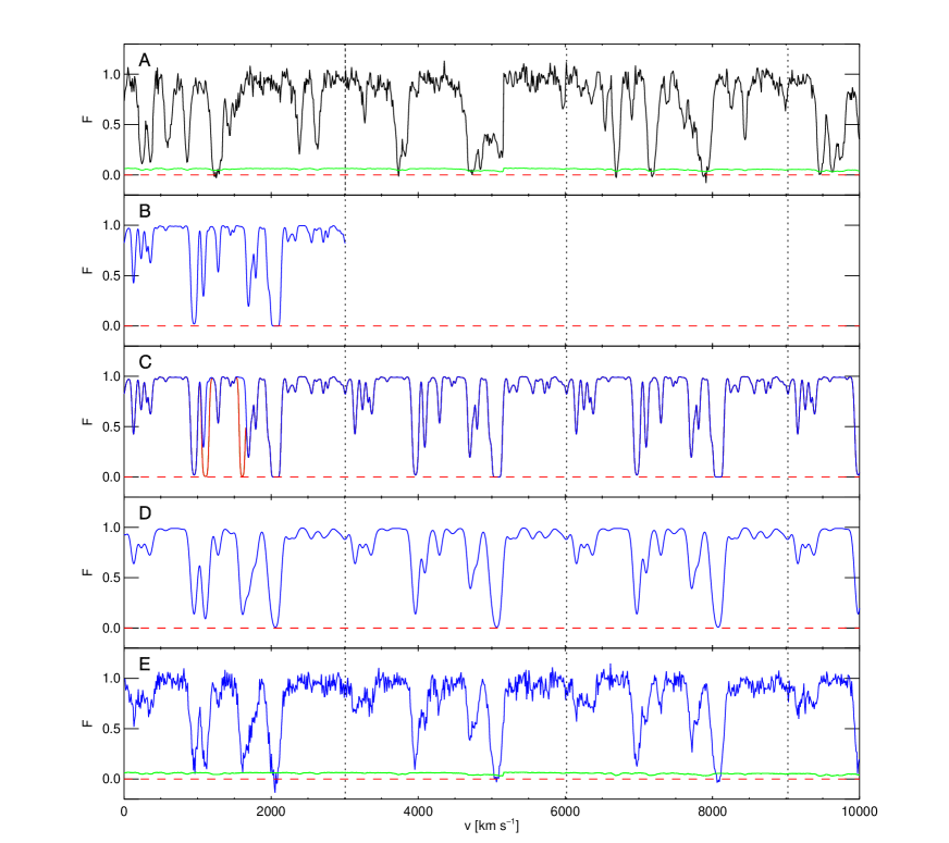
Figure S4: The main steps in our forward-modelling procedure. The upper panel shows the spectrum of the quasar SDSS J111610.69+411814.4, observed with ESI. The zero level and the estimated noise are marked in dashed red and green, respectively. Vertical dotted lines divide the spectrum in regions of 30 Mpc$/h$, which is the length of the box size of our N-body simulation on which our semi-numerical models are based. The second panel shows in blue a simulated spectrum from one of these models, with $\lambda_{P}=85$ kpc, $T_{0}=20000$ K and $\gamma=1.6$. In the third panel the synthetic spectrum is periodically replicated and the optical depth of metal lines (red) and LLS (green) is added (we have chosen a particular sight line where both contaminants are present for illustration purposes). In the fourth panel we show the extended spectrum convolved with a Gaussian kernel with FWHM matched to the resolution of the spectrograph, which in this case amount to 64 km s^-1. In the last panel we add noise pixel by pixel according to the pipeline estimate at each wavelength. The zero point of the velocity scale is arbitrarily set to the minimum redshift of the segment (for the observed spectra) or to the edge of the box (for the simulations).

A further complication stems from the wavelength dependence of the noise, which is typically higher at smaller $\lambda$, because of the lower spectrograph sensitivity in the near-UV. We model this wavelength dependence by adding Gaussian noise to our model spectra with a standard-deviation given by the wavelength dependent 1$\sigma$ noise vector of each spectrum, produced by the data reduction pipeline. In order to add wavelength dependent noise in this way, we need to somehow extend the simulated sight lines, which are only $30$ Mpc$/h$ long ($3008$ km/s at $z=2$), so that they are comparable to the length of the observed spectral segments ($\sim 15000$ km/s for $\Delta z=0.2$ at $z=3$). This is done by periodically replicating each simulated spectrum until its size matches that of the forest segment on which it is calibrated (see Fig. S4). This procedure is allowed because the periodic replication does not affect the phase distribution of the modes, but it is effectively used as a convenient resampling of the same sight lines under different noise conditions, in order to take into account the wavelength-dependent sensitivity of the instruments.

The flux of the spectrum obtained after the periodic replication is finally rebinned on to the same pixel grid as the observed spectrum, which is always coarser than the one used in our simulation. Once this is done, we are able to generate Gaussian noise, matched pixel by pixel, to the estimated wavelength-dependent noise of the data. As our quasar spectra have been continuum normalized, the noise vectors are also divided by the same continuum such that the appropriate level of noise is added.

5.5 Forward-Modeling of the Simulation

The methodology described in the three previous paragraphs constitutes our forward-modelling procedure, which alters our simulated spectra to have the same properties as real spectra observed through a telescope with finite resolution and integration time, and containing contaminant metal lines and LLSs. Our forward-modelled simulations can be directly compared to observations, enabling our statistical phase angle PDF analysis and thermal parameter study. As we have explained above, the forward-modelling procedure is tailored to individually reproduce the properties of each spectrum in each quasar pair, and must be applied to all the IGM models that we want to test. The general procedure that we follow to perform the phase angle PDF analysis on our dataset is summarised below.

Our goal is to evaluate the likelihood in eqn. (S3) for any thermal model $\left\{T_{0},\gamma,\lambda_{P}\right\}$ using phase differences from our pair sample. Given a quasar pair separated on the sky by an angle $\psi$, with overlapping ${\rm Ly\alpha}$ forest intersecting one of our redshift bins $Z=[z_{1},z_{2}]$, we have to forward-model the simulated spectra and to determine the phase angle PDF for an IGM model with $\left\{T_{0},\gamma,\lambda_{P}\right\}$ at each $k$ for the appropriate impact parameters. This operation is structured as follows:

• We determine the overlapping portion of the ${\rm Ly\alpha}$ forest of the two QSOs which intersects the redshift bin $Z$. This segment will have a comoving separation varying with redshift as $r_{\perp}(z)=D_{A}(z)\psi(1+z)$ (see section § 5.2).

• We generate 400 pairs from the simulated box distributed in transverse separations $r_{\perp}$ depending on $r_{\perp}(z)$ as described in § 5.2.

• The optical depth of the total sample of 400 sight lines is renormalized in order to match the literature value of the mean ${\rm Ly\alpha}$ flux of the central redshift of the bin.

• All 400 pairs are forward-modeled according to the properties of the two observed spectra in the pair, which have in general different resolutions and S/N. This is done through the following four steps:

  1. Simulated spectra are periodically replicated until they match the length of the observed segments of forest.

  2. The optical depth of metal lines and LLSs is added to the sight lines.

  3. The spectra are convolved with a Gaussian kernel with FWHM set by the spectral resolution.

  4. Simulated spectra are then rebinned onto the same pixel grid as the data.

  5. Gaussian uncorrelated noise is added to the simulated flux with a standard-deviation determined by the $1\sigma$ noise vector of the observed spectrum.

• We calculate phase angle differences from the simulated pairs and estimate the wrapped-Cauchy concentration parameters $\zeta$ (see eqn. (S2)) at each bin in $k$. We thus predict the phase angle PDF $P_{WC}(\theta(k))$ as a function of $k$ for the considered pair. Having rebinned the sight lines at step 3, we have to calculate phases with the LSSA method as we do with data.

  This procedure is then repeated for each observed quasar pair, for each IGM model, and in each redshift bin. Given the forward-modeled phase angle PDFs, we can then compute the likelihood in eqn. (S3) by taking the product over all quasar pairs and over all modes sampled by a given quasar pair. The product over modes is evaluated only for modes below the limiting wavenumber $k_{R}$, which is set by resolution. This provides values of the likelihood function for all pairs over the entire model parameter space, allowing us to infer the thermal properties of the IGM at each redshift.

6 MCMC Exploration of the Phase Angle PDF Likelihood

Our parameter grid consists of 400 models in the space defined by $T_{0},\gamma,\lambda_{P}$. Based on previous measurement and on a preliminary analysis, we adopt the following flat prior on the parameters: $T_{0}\in 5000-30000$ K, $\gamma\in 0.5-2.0$, $\lambda_{P}\in 22-200$ kpc. The lower limit in $\lambda_{P}$ is dictated by the resolution of our dark-matter simulation: according to a previous test (see RHW) we can only study smoothing scales larger than the mean interparticle separation. We first calculate 50 sets of smoothed density and velocity skewers from our dark-matter simulation, as described in § 5.1, corresponding to 50 different choices of $\lambda_{P}$, logarithmically spaced between 20 kpc and 200 kpc.

We build our grid of models to efficiently sample not only the 3D thermal parameter space, but also the projected 2D and 1D subspaces of the parameters. Regular Cartesian grids do not perform well because when projecting a cubic grid onto a plane all points in a row are projected to a single point. The algorithm adopted to create the parameter grid is the following:

• The parameter space is broadly subdivided in $8\times 4\times 4=128$ bins (in $\lambda_{P},T_{0},\gamma$).

• The first point is chosen randomly in the center of one of the 128 bins.

• Each of the next points is then added to one of the bins $\tilde{B}$ with the smallest number of points in it (chosen randomly).

• Once the bin $\tilde{B}$ is chosen, we pick one of the discrete values of $\lambda_{P}$ within that bin. We always choose the value of $\lambda_{P}$ with the smallest occurrence within the set of the previous points.

• We then define a $4\times 4$ subgrid in the $T_{0}$-$\gamma$ plane, limited to the area defined by the projection of $\tilde{B}$.

• Analogously to what we have done with $\lambda_{P}$, we pick one of the 16 subcells and assign to the current point the value of $T_{0}$ and $\gamma$ at its center. The subcell is chosen to be the least represented among the previous points.

• This process is repeated until we have reached the desired number of points in the parameter space.

In this way we define a grid of 400 points in $T_{0},\gamma$ and $\lambda_{P}$ for all four redshift bins. We then calculate the phase angle PDF likelihood of all the models as described in the previous section, then we use Gaussian process interpolation to interpolate this likelihood to any arbitrary point in the parameter space. Gaussian processes are a statistical method to interpolate irregular grids, which assume that the quantity to interpolate is the result of a stochastic process characterized by a Gaussian distribution. Detailed explanations and its application to the matter power spectrum can be found in  (?, ?, ?).

In our case, the only input for the Gaussian process interpolation is the choice of the ’smoothing lengths’, which quantify the extent of the correlation of the likelihood along each dimension of the parameter space. We choose these smoothing lengths to be a multiple of the average spacings of our parameter grid. The choice of these smoothing lengths is somewhat arbitrary, but we checked that the inferred posterior distributions of thermal parameters do not change in response to reasonable variations of these smoothing lengths.

We employ a publicly available MCMC package emcee  (?). The results of the MCMC runs are shown in Fig. 3 of the main text, in the form of 65% and 95% confidence levels in the $\gamma$- $\lambda_{P}$ and $T_{0}$-$\lambda_{P}$ planes, and in the form of posterior probability distribution of $\lambda_{P}$.

7 Visual Comparison of the Phase Angle PDF to Models

Our parameter estimation is based on MCMC sampling of a multi-dimensional parameter space, which delivers a posterior distribution for $\lambda_{P}$, $T_{0}$, and $\gamma$. Nevertheless, it is instructive to construct visual data for model comparisons. This is challenging because the information in the phase angle PDF is spread out across many $k$ and $r_{\perp}$. So we adopt a procedure of binning modes and separations together, which also allows us to overplot similarly binned phase angle PDFs from our models calibrated with our forward-modelling procedure. (§ 5.1).

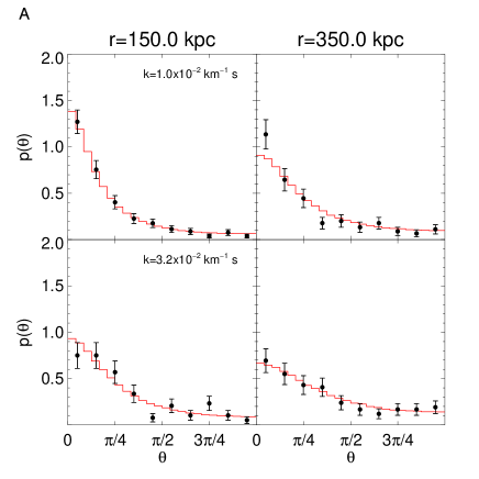
Figure S5: Observed phase distributions. Black points: Phase difference PDF calculated from real data calculated at redshift $z=2,2.4,3,3.6$ (from left to right and from top to bottom). In each of the four plots the phase difference are binned in $k$ and $r_{\perp}$ (see text for the exact definition of the bins). The central values of the $r_{\perp}$ bins are reported at the top of each column, and the central values of the $k$ bins are reported in the legend of the left columns. Error bars are calculated assuming a Poisson distribution. Red histogram: the phase difference PDF of the best-likelihood model, calculated after fully modelling noise, resolution and contaminants, as described in the text.

The measured phases are binned and plotted in Fig. S5 in the same way described in § 4.3, which we used to produce Fig. S3. In this case, we only use two bins for $k$ and two bins for $r_{\perp}$, for all four redshift bins in our analysis. The $k$ bins are defined by the intervals $0.005-0.02,0.02-0.05$ km^-1 s (from top to bottom in each of the four subplots), and the $r_{\perp}$ bins by $50-250,250-450$ kpc (left to right). The values quoted by the labels in the figure are the (rounded) central values of the bins. In constructing this plot from the data, we are grouping together phases from different pairs, with different noise and resolution properties. In order to sensibly compare these observed distributions to our model, we employ our forward-modelling procedure. The forward-modelling approach, summarized in § 5.5 creates a sample of mock spectra which exactly reproduces the distribution of separation, wavenumber, noise and resolution of the data, but exploiting the much larger path length available in the simulations, resulting in a much smaller statistical error. For any model, this mock data sample can therefore be used to facilitate a meaningful visual comparison between models and data. After forward-modelling a simulation, we calculate the phase differences in the synthetic pairs and group them in the same exact way as has been done for the data. The phase angle PDFs of the similarly binned mock data are shown as the red histograms in Fig. S5. For this comparison we have chosen the model in the parameter grid that provides the maximum likelihood (at each redshift) evaluated as in eqn. S3.

Fig. 2 is built in an analogous way, except that we define only one single bin which encompasses all the phases in each redshift bin, both for the data points and for the simulated models. The shaded regions in that figure are calculated by taking as the boundaries the two semi-numerical models with the closest $\lambda_{P}$ to the 16% and 84% percentiles of the $\lambda_{P}$ posterior distribution. Given the weak dependence on $T_{0}$ and $\gamma$, we choose the values of these parameters to be as close as possible to $T_{0}=15000$ K $\gamma=1$, i.e. around the middle of the allowed range.

8 Quantifying Systematic Errors

The phase angle PDF method has not been previously analysed for the impact of systematics on it have not been previously considered. In this section we assess the robustness of our results with respect to possible sources of systematic error. First we consider the sensitivity of our results to the fit of the unabsorbed continuum level (§ 8.1), then we determine how sensitive we are to assumptions made about the the spectral resolution (§ 8.2) and on our knowledge of the noise level (§ 8.3). In § 8.4 investigate the impact of metal lines and LLS in decreasing the transverse coherence of the ${\rm Ly\alpha}$ forest in quasar pairs, and determine how how much our results would change if the assumed abundance of these contaminants is varied.

8.1 Continuum Fitting

Phase differences are insensitive to the normalization of the flux, and this fact led us to argue that they are robust against uncertainties in our continuum fitting. This statement would be mathematically exact if continuum error could be described as simply a multiplicative uncertainty in the flux normalization. However, in realistic spectra the true underlying continuum may have emission lines or a different slope than the one estimated by continuum fitting, but as long as these features affect scales larger than the largest modes we analyse ($v\gtrsim 1500$ km/s) we expect little effect on the phase angle PDF. To prove this explicitly we adopt a conservative approach: we calculate the phase angle PDF directly from the observed flux without fitting the continuum of the spectra at all. We then compare the results with the standard case of continuum-normalized spectra. The results are shown in Fig. S6 for our redshift bin at $z=2$. The agreement between the non-normalized flux and the standard continuum-normalized case is clear at all $r_{\perp}$ and $k$ (binned as in Fig. S3). The differences between the best-fit wrapped-Cauchy distributions, plotted as the solid lines are even smaller. The only significant discrepancy occurs in a single bin ($r_{perp}=250$ kpc, $k=8.9\times 10^{-3}$ s/km, top center), which may be caused by a strong feature at large scales in the non-normalized continuum of a spectrum. This difference is however smaller than the statistical error indicated by the errorbars.

8.2 Resolution

In § 3 we described how we used the line-of-sight flux power spectrum from a distinct sample of high-resolution quasar spectra to calibrate our resolution estimate. In this section we present a test to show that our results are not significantly impacted by the exact value of the resolution that we assume. This test is performed by repeating the measurement after varying our assumptions on the spectral resolution, exploring the cases where it is chosen to be 10% higher or lower then the default value we adopted.

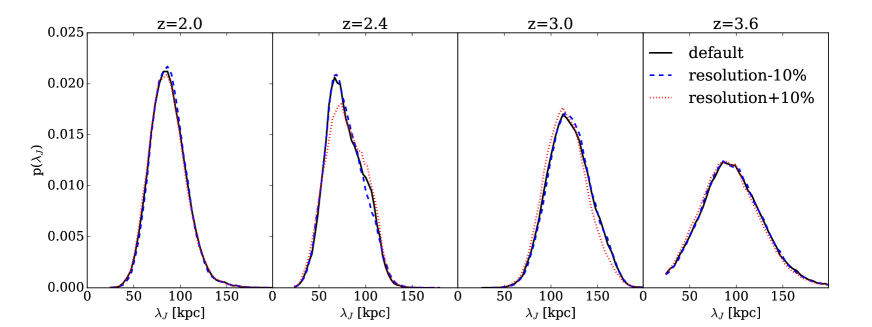
Figure S7: Impact of the uncertainty on resolution modeling. Posterior probability distribution for $\lambda_{P}$ under different assumptions regarding the resolution. The default run is shown in blue, where the FWHM is rescaled to achieve a good match of the flux power spectrum, as explained in the text. The green and the red curves show cases where the resolution is assumed to be 10% lower or higher, respectively. At all redshifts the variation of the median value in the posterior distribution of the pressure smoothing scale is less than 1%, more than an order of magnitude smaller than the statistical error on $\lambda_{P}$. The exact values are reported in Table S2.

The results of this resolution test are illustrated in Fig. S7. The bias in $\lambda_{P}$ resulting from the resolution correction are in all cases a tiny fraction of our statistical errors. We calculate the differences between the median of the posterior distribution of $\lambda_{P}$ in the default run and in these two test runs. We choose the the larger of these two differences as our estimate for the error associated with our uncertain knowledge of the resolution, which amounts to less than 1% for all redshift bins (Table S2). These errors are an order of magnitude smaller than the purely statistical uncertainties, which we quantify as the difference $\Delta^{+1\sigma}\lambda_{P}=\lambda_{P,84}-\lambda_{P,50}$ between the 84th percentile and the median of the posterior distribution of $\lambda_{P}$, and the difference $\Delta_{-1\sigma}\lambda_{P}=\lambda_{P,50}-\lambda_{P,16}$ between the median and the 16th percentile (the relevant percentile values are listed for all redshift bins in Table S2). We therefore conclude that our measurement is not substantially affected by our lack of knowledge of the exact value of the spectral resolution. This partly follows from the mathematical properties of phases that they are invariant under convolution of the function with symmetric kernels (see RHW for more details). Furthermore, we are excluding from the analysis the high-$k$ Fourier modes beyond the resolution limit (see § 5.4). The possibility of narrowing the dynamic range in order to exclude unresolved modes is one of the main motivations to adopt a Fourier-space statistic.

8.3 Noise

We adopt the same approach described in the previous section to quantify the impact of uncertainties in our noise model on our results. In particular we want to understand the bias on $\lambda_{P}$ we would obtain if the noise model estimated by our data reduction pipeline is incorrect, which would result in a systematic error in our forward-modelling procedure. If our estimates of the noise are too low, the coherence of the quasar pairs in our models would be higher than they actually are in reality. As a consequence, the lower coherence of the data relative to the (incorrectly modelled) more coherent models would be interpreted as a smaller pressure smoothing scale. To quantitatively assess the magnitude of this effect, we repeat the phase analysis under the assumption that the noise level is 10% higher or lower than the value estimated by our data reduction pipeline.

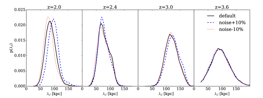
Figure S8: Impact of the uncertainty on noise modeling. Same as Fig. S7, but this time adjusting the noise level in the simulated spectra by 10%. The variation of the median $\lambda_{P}$ is different depending on the redshift and on the data quality. The precise values are reported in Table S2.

The results are shown in Fig. S8. The discrepancy caused by varying the noise by 10% from the pipeline estimates differs substantially in the four redshift bins. This is caused by the variation in the signal-to-noise ratio within the data sample. Although the lower redshift quasar pairs in our sample tend to be brighter on average, the spectrograph throughputs degrade rapidly toward the UV and the signal from the ${\rm Ly\alpha}$ forest is weaker at lower redshift. There is therefore no reason to expect a clear redshift trend. Similar to the previous section, we estimate the associated uncertainties as the highest of the two differences between the median values of the posterior distribution of $\lambda_{P}$ in the $\pm 10\%$ test runs and the default case, at each redshift. The values are reported in the fifth column of Table S2. The highest variations (9.9% and 4.7%) occur at $z=2$ and $z=3$, respectively, while at $z=2.4$ and $z=3.6$ the estimated uncertainty is below the percentage level.

8.4 Metal Lines and Lyman Limit Systems

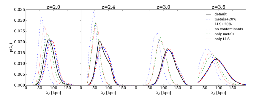
Figure S9: Effect of contaminants modeling. Posterior probability distribution for $\lambda_{P}$ under different assumptions regarding the properties of the contaminants. Our default run is represented by the blue line. The cyan dot-dashed line represent the case where both metals and LLS are completely neglected. The effect of metals alone is demonstrated by the violet dashed curve, where LLS are not included. Conversely, the orange dotted lines show models containing only LLS contamination. Contamination in the models can lead to underestimation of the smoothing scale if not corrected. We tested the stability of our results with respect to the modelling of contaminants, by varying by 20% the abundance of metal lines (green curves) or LLS (red). The consequent increase in the median value of the $\lambda_{P}$ posterior distribution is at most 9% (see text for a complete discussion).

The last systematic we need to address is the contamination due to metal lines and LLSs. In our default forward model both of these components are added to the synthetic spectra as described in § 5.3. In Fig. S9 we present the resulting posterior distributions for $\lambda_{P}$ when one or both of these contaminants are neglected, compared to the default case where they are fully taken into account. It demonstrates that the pressure smoothing scale is significantly underestimated if this effect is not modelled, and the precision is overestimated. The effect is similar but smaller if only one of the two type of contaminants is considered, as shown by the posterior distribution of $\lambda_{P}$ when only LLS or metal lines are included.

We reiterate that we add these contaminants to simulated pairs in a completely random uncorrelated fashion, whereas in reality, given the small impact parameters probed by our quasar pair sight lines, metals and LLSs could be significantly auto-correlated  (?, ?, ?), and LLSs may also cross-correlate with the Ly$\alpha$ forest absorption  (?). If such correlations exist in reality and are strong enough to influence the phase coherence, it would make the real quasar pair data more coherent compared to our models, where we have assumed a maximally incoherent distribution of metals and LLSs. In that case the mismatch between metal and LLS coherence in the data relative to the model, would be interpreted as a higher pressure smoothing scale in the data, i.e. we would overestimate $\lambda_{P}$.

To quantify the impact of our treatment of metals and LLSs on our results we modify our forward modelling procedure, increasing the respective abundance of metals and LLS by 20%. The posterior probability distribution for $\lambda_{P}$ obtained from our MCMC is then compared to our default forward model, analogous to our treatment of resolution and noise in the the previous sections.

To increase the LLS abundance, we simply scale the factor $l_{z0}$ in eqn. S28 up by 20%. In this way we increase the occurrence of LLS at all column densities by the same amount. Metal line contamination is artificially enhanced as follows. As described in § 5.3, metals are injected into our spectra by sampling co-eval spectral segments of lower-$z$ quasars, for which the metal lines are not blended with the ${\rm Ly\alpha}$ forest. In practice, only a fraction of these spectral segments contain metal lines. To increase the metal line abundance in our mock spectra, we simply artificially increase the probability of picking a segment with metal lines by 20%. On average this procedure increases the abundance of metal lines in the models by the desired amount. The results are shown in Fig. S9 and summarized in the last two columns of Table S2.

The variation on the estimated $\lambda_{P}$ (i.e. the median of the posterior distribution) caused by a change in metal or LLS abundance by 20% is in all case less than 10%, with a decreasing trend towards high redshift. These discrepancies are taken as an estimate of the error associated with the uncertainty on metal contamination and LLS. When added in quadrature to the purely statistical uncertainty, they only contribute to the total error by a small amount.

8.5 Systematic Uncertainties: Summary

In this section we have tested the potential biases associated with uncertainties on spectral resolution, noise, metal contamination and LLS. In Table S2 we report all the corresponding errors we estimated. These errors are always calculated as the difference between the median of the posterior distribution of $\lambda_{P}$ in the default case and the median in a test case where these effects are varied. When we have two test cases where we vary the systematic in opposite directions (as done for the noise and the resolution), we conservatively take the maximum of the two differences. We report these uncertainties, organized by type and by redshift, in Table S2. In calculating the total error (i.e. statistical+systematic, last column in Table S2), we add the systematic errors in quadrature to the purely statistical uncertainties from the MCMC posterior for $\lambda_{P}$ for our default case. The latter are quantified as the difference $\Delta^{+1\sigma}\lambda_{P}=\lambda_{P,84}-\lambda_{P,50}$ between the 84th percentile and the median of the posterior distribution of $\lambda_{P}$, and the difference $\Delta_{-1\sigma}\lambda_{P}=\lambda_{P,50}-\lambda_{P,16}$ between the median and the 16th percentile. The impact of systematic errors is illustrated by the black extensions to the statistical errorbars (red) shown in Fig. 4 of the main text, which have been calculated in this way.

9 The Smoothing Scale in Hydrodynamical Simulation

As we discussed in § 5.1, we opt for a more flexible semi-numerical model of the thermal state of the IGM based on collisionless dark-matter only simulations to conduct our data analysis. The reason for this is that it is a great computational challenge to simulate the full set of thermal histories that could give rise to a large range of pressure smoothing scale that the data analysis requires. In this section we discuss an ensemble of full hydrodynamical simulations that we run. Our approach is to treat the hydro simulation as a mock dataset, and then run our phase angle PDF method on the hydro simulations to infer the smoothing scale in the context of the DM models. We show that there is a tight relation between the semi-numerical pressure smoothing scale in the DM models, and the analogous scale in the hydro simulation. This forms the basis for Fig. 4 in the main text, where we applied the phase angle PDF method to a set of hydro simulations, and we provide the details of how that Figure was constructed.

9.1 Hydrodynamical Simulations

For the hydrodynamics simulations, we use Nyx, an N-body/gas dynamics code for large-scale cosmological simulations  (?, ?). It follows the temporal evolution of dark matter gravitationally coupled to an inviscid ideal fluid in an expanding universe. The gas dynamics are evolved using a finite volume approach on a three-dimensional Eulerian grid. Dark matter is represented as discrete particles moving under the influence of the gravitational field. The same mesh structure that is used to update fluid quantities is also used to compute the gravitational field and to evolve the particles via a particle-mesh method. Adaptive mesh refinement (AMR) can be used for the hydrodynamics and self-gravity solver. However, to model Lyman-alpha absorption, it is most important to correctly describe the thermodynamic state of the IGM at relatively low densities, from below the cosmic mean, to about ten times the mean density. Because these are vast regions of the universe, employing AMR to resolve them does not provide a significant advantage. In addition, these regions are devoid of galaxies, thus physical processes related to galaxy formation are not expected to play a significant role in determining thermal state of the IGM  (?). For these reasons, we do not use the AMR capability in these runs. The simulations we run are periodic-boundary cubes, 20 Mpc$/h$ on a side, with $1024^{3}$ cells, resulting in approximately 20 kpc/$h$ cell size. This box size and resolution are chosen in order to achieve convergence in the low density IGM  (?). In addition, we have verified that the phase angle PDF determined from pairs of spectra is converged in simulations of this resolution, and that it is insensitive to the box size. In these simulations we use the following cosmological parameters, consistent with the latest cosmological constraints from the CMB  (?): $\Omega_{m}=0.3192,\Omega_{b}=0.04964,\Omega_{\Lambda}=0.6808,h=0.67038$ and $\sigma_{8}=0.826$. Note that these parameters are slightly different than those used in the dark-matter simulations described in § 5.1. In any case, changes in the dark-matter models only affect the definition of $\lambda_{P}$, not its physical interpretation and its connection to the thermal history which is instead calibrated on hydrodynamical simulation, as it will become clear in section § 9.2. In any case, the sensitivity of our results to the cosmological parameters is weak, as shown in § 9.4.

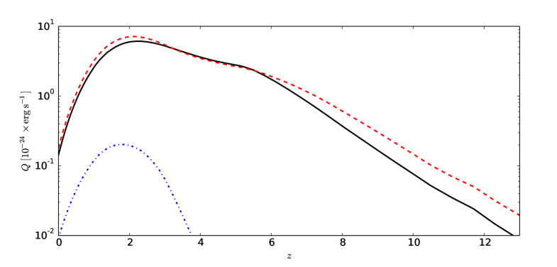
Figure S10: Photoheating rates per ion in our models for the species H i (black), He i (red dashed) and He ii (blue dotted) as a function of redshift in the HM12 model. These rates form the basis of the range of thermal histories that we explore with our hydrodynamical simulations. In particular, in the late reionization heating model presented in the main text the photoheating rates are the same for $z\leq 7$ and set to zero for $z>7$, while in the increased heating model they are multiplied by three at all redshifts.

As described in  (?, ?), our simulations account for the radiative heating and cooling via source terms in the energy equations. The gas in the simulations is assumed to be optically thin and in ionization equilibrium with a spatially uniform ultraviolet background (UVB), which results from the collective emission of galaxies and quasars. In this work, we use photoionization and photoheating rates from the  (?, HM12, see Fig. S10) synthesis model which results in an IGM which is already heated up to $T\sim 10^{4}~{}{\rm K}$ at $z=15$  (?), which is also the de facto redshift of reionization in simulations where the HM12 photoionization and photoheating rates are employed. To study the impact of thermal and reionization history on the pressure smoothing scale, we also consider models where the photoheating and photoionization rates are set to zero beyond some given $z_{\rm reion}$ . At $z_{\rm reion}$ the HM12 uniform UVB and photoheating rates are then switched on, and used for the rest of the time evolution. In the main text we compare our results with the standard HM12 model, a model where the reionization redshift is $z_{\rm reion}$ = 7 (”late reionization heating”) and one where the heating rates are increased by a factor $A=3$, to test whether a increased-heating scenario might be consistent with the temperature measurements from  (?). Rescaling heating rates is a standard phenomenological approach for modelling the thermal history, which was first adopted in  (?). Further details of the three simulations we run are specified in Table S3.

We analyzed a set of 13 hydrodynamical simulations, where a wider range of heating parameters and reionization redshifts are explored, resulting in a larger variation of the pressure smoothing scale. Beside the rescaling factor of the heating rates $A$ and the reionization redshift $z_{\rm reion}$, we also consider models where the heating depends on density according to $\Delta^{B}$  (?), with $B$ being a free parameter. The parameters of this set of simulations are reported in Table S4. This allows us to better characterize the relation between the parameters of the thermal history in hydrodynamical models and the smoothing scale of the IGM measured with phase differences and defined in our semi-numerical dark-matter models.

9.2 Phase Analysis of the Hydrodynamical Simulations

In this section we describe how we apply the phase angle PDF method to a set of mock quasar pairs drawn from the hydrodynamical simulations. The goal is to characterize the pressure smoothing of the IGM in the hydrodynamical models using the transverse coherence of phases, consistent with what we have done with the observational data. This establishes the foundation for a meaningful comparison between our measurement and the predictions of the hydrodynamical simulations we run.

As explained in § 5.1, the phase angle PDF analysis is calibrated on a set of semi-numerical models where the smoothing is imposed by convolving the dark matter density distribution with an approximately-Gaussian kernel. This approximation allows us to relate an observable, namely the distribution of phase differences in quasar pairs, to a definition of smoothness in the density field ($\lambda_{P}$). Since this relation is used to characterize the observational results described in the main text, we apply it to the Ly$\alpha$ forest skewers drawn from the the hydrodynamical simulations in order to define the pressure smoothing scale of the different hydro simulations that we consider.

Schematically, the procedure we adopt can be described as follows:

• We draw 10,000 synthetic pairs of skewers from the hydrodynamical simulation, choosing separations in multiples of the grid spacing 27.9 kpc, for a total path length of 140 Gpc. This constitutes our mock (noiseless) dataset.

• We calculate phase differences for all the pairs in the mock sample, imposing the same limits on the dynamical range as in the data ($k<0.1$ s/km).

• We evaluate the likelihood of the obtained set of phases using the probability distributions predicted by our grid of DM-based models at the same transverse separations.

• The pressure smoothing scale of the simulation is defined as the pressure smoothing scale $\lambda_{P}$ of the maximum-likelihood DM model. To achieve better precision we use Gaussian processes to interpolate the likelihood in parameter space.

We repeated this method for all three simulations listed in Table  S3 and at all four redshift bins. Simulations snapshots are approximately drawn from the central redshift of the four measured bins, more precisely at $z=2,2.4,3.0,3.6$. These values are used to determine the simulation predictions between $z=2$ and $z=3.6$ in Fig. 4. Below we explain how we extrapolate these prediction to higher and lower redshift.

9.3 Definition of the Pressure Smoothing Scale in Hydrodynamical Simulations

Whereas $T_{0}$ and $\gamma$ can be easily estimated by fitting the temperature-density distribution with a power law, defining the pressure smoothing scale in hydrodynamical simulations is not trivial. The gas density power spectrum does not exhibit a sharp pressure smoothing cutoff, because dense gas in collapsed halos dominates the small-scale power masking pressure smoothing effects  (?). A possible solution has been proposed in  (?), where they define a new quantity, the real-space ${\rm Ly\alpha}$ flux $F_{\rm real}$, which naturally suppresses the impact of this dense gas, and is thus robust against the poorly understood physics of galaxy formation, revealing pressure smoothing in the diffuse IGM. The $F_{\rm real}$ field is calculated as the transmitted flux of ${\rm Ly\alpha}$ photons in the fluctuating Gunn-Petersson approximation, defined by

$$F_{\rm real}(x)=\exp\left[-\frac{3\lambda^{3}_{\alpha}\Lambda_{\alpha}}{8\pi H(z)}n_{\rm H{\sc i}}\right]$$ (S32)

where $\lambda_{\alpha}=1216$Å is the rest-frame ${\rm Ly\alpha}$ wavelength, $\Lambda_{\alpha}$ is the Einstein $A$ coefficient of the transition, $H(z)$ is the Hubble parameter and $n_{\rm H{\sc i}}(x)$ is the neutral hydrogen number density at the point $x$. In the optically-thin regime, where $n_{\rm H{\sc i}}\propto\rho^{2}$ this is a non linear transformation of the density field that suppresses high densities, but preserves isotropy.

In  (?) it is shown that $F_{\rm real}$ power spectrum is accurately described by a simple fitting function with cutoff at $\lambda_{P,{\rm sim}}$:

$$\Delta_{F}(k)=Ak^{n}\exp[-(k\lambda_{P,{\rm sim}})^{2}],$$ (S33)

where $A$, $n$ and $\lambda_{P,{\rm sim}}$ are the free parameters. This characterization allows a rigorous quantification of the pressure smoothing in hydrodynamical simulations. They have also shown that the value of $\lambda_{P,{\rm sim}}$ is strictly dependent on the thermal history, confirming its physical origin from the pressure smoothing of the baryons.

It is natural to consider the relation between this definition of pressure smoothing and the one coming from the phase angle PDF analysis described in § 9.2, where the pressure smoothing scale is determined by applying our phase-angle PDF method, calibrated with semi-numerical dark matter models, to pairs of Ly$\alpha$ forest skewers drawn from hydrodynamical simulations. A strong correlation between the two would be a convincing argument that our dark-matter based modeling approach is actually measuring the small-scale coherence of the baryon density field, which is determined by the thermal history of the gas. To verify this, we apply our phase angle PDF analysis to the extended set of 13 hydrodynamical simulations described in Table S4. We use the phase angle PDF analysis method described in § 9.2 to ’measure’ $\lambda_{P}$ for each simulation model. We then compute the 3D power spectrum of $F_{\rm real}$ in each of these hydrodynamical models. The expression in eqn. S33 is fitted to these power spectra, providing an estimate of $\lambda_{P,{\rm sim}}$ for each model.

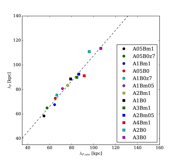
Figure S11: Pressure smoothing in hydrodynamic simulations. The points show the relation between the pressure smoothing scale $\lambda_{P,{\rm sim}}$ of the hydrodynamical simulation defined by the cutoff in the power spectrum of $F_{\rm real}$ ($x$ axis), and the scale $\lambda_{P}$ derived by the phase analysis of a mock sample of pairs extracted from the same simulations ($y$ axis), calculated at $z=3$. The dashed line represents a polynomial fit to the distribution. The legend lists simulations from Table S4, sorted in increasing order of $\lambda_{P,sim}$, such that the points appear left to right in the plot.

At the end of this procedure we have a set of values of $\lambda_{P}$ (from phases and DM modeling) and of $\lambda_{P,sim}$ (from the fit of the $F_{\rm real}$ power spectrum in hydro simulations) for all of the thermal models. We show a comparison of these two quantities at $z=3$ in Fig. S11. There is a clear monotonic trend between the two measures of pressure smoothing, and an almost one-to-one relation with a scatter of less than 5% (see Table S4 and Fig. S11), indicating that they are a proxy for the same physical quantity. Hence we argue that the properties of $\lambda_{P,{\rm sim}}$ analysed in  (?) are shared by $\lambda_{P}$. In particular this demonstrates the sensitivity of our measured value of $\lambda_{P}$ to the thermal history of the IGM.

We perform a linear fit of the relation between $\lambda_{P}$ and $\lambda_{P,{\rm sim}}$ at the four redshifts used for our measurement. We then assume that the fitted functions at $z=2$ and $z=3.6$ are a good approximation for $\lambda_{P}(\lambda_{P,{\rm sim}})$ at redshift lower and higher than the four bins, respectively. In this way we can use the values of $\lambda_{P,{sim}}$ determined at each snapshot of the simulations in order to extrapolate the model predictions for $\lambda_{P}$. This is done purely for illustrative purposes, as we do not have a measurement to compare with outside of the redshift interval probed by our data $z\in[1.8,3.9]$. These extrapolations are shown in Fig 4 for redshifts $z<2$ and $z>3.6$.

9.4 Convergence and Sensitivity to Cosmological Paramaters

In this section we quantify the level of convergence of the pressure smoothing scale in hydrodynamical simulations with respect to resolution and box size, and also investigate its dependence on the cosmological parameters. We will focus here on the hydrodynamical runs because the dark matter simulation (described in § 5.1) has both a higher resolution and a larger size, and its resolution convergence criteria were already tested in  (?).

Our approach is to apply exactly the same procedure described in § 9.2 in order to estimate $\lambda_{P}$ for a suite of simulations where resolution, box size, or cosmological parameters are varied, and then compare the results with the value of the default hydrodynamical simulations that we compared to our data. All tests are performed at $z=3$.

9.4.1 Resolution Convergence

The resolution convergence test is performed on three simulations in a 10 Mpc$/h$ box. The default setting is represented by a run with $512^{3}$ cells, which has the same cell size of our standard boxes ($l_{c}=$19.5 kpc$/h$). We then have two boxes with $256^{3}(l_{c}=39.1$ kpc$/h$) and $1024^{3}(l_{c}=9.8$ kpc$/h$) cells. The initial conditions and thermal histories are the same in the three cases. The cosmology is different than the one employed in our thermal grid (§ 9.1), as these models were run with cosmological parameters consistent with the Wilkinson Microwave Anisotropy Probe (WMAP) 7-year data  (?): $\Omega_{m}=0.275,\Omega_{b}=0.046,\Omega_{\Lambda}=0.725,h=0.702$ and $\sigma_{8}=0.816$.

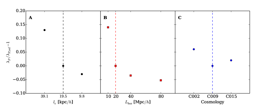
Figure S12: Results of the convergence tests. All the plotted values of $\lambda_{P}$ are calculated at $z=3$ via a phase analysis of synthetic pair spectra, as described in § 9.2. Panel A, resolution test: Relative difference in $\lambda_{P}$ with respect to the default run (marked by a vertical dashed line) as a function of the cell size $l_{c}$ for three simulations in a 10-Mpc$/h$ box. Panel B, box size test: relative difference in $\lambda_{P}$ as a function of the box size $L_{box}$. The default run, marked by the vertical dashed line, has a box size of 20 Mpc. The resolution of the four simulation is kept constant by choosing the appropriate number of cells. Panel C, cosmology dependence: sensitivity of the estimated $\lambda_{P}$ to the cosmological parameters relative to the fiducial model (C009, blue dashed line). The three points represent three models in which cosmological parameters are varied consistently with the current observational constraints (see text for details).

The relative discrepancy of $\lambda_{P}$ (with respect to the default run) as a function of the cell size $c_{l}$ is shown in the left panel of Fig. S12. While the lowest-resolution run is clearly not converged, the discrepancy between the default and the high-resolution simulations is approximately $3\%$, which is an order of magnitude lower than our statistical errors.

9.4.2 Box Size Convergence

We examine four hydrodynamical models with box size $L=10,20$ (reference value) $,40,80$ Mpc$/h$ and number of cells $n=512^{3},1024^{3},2048^{3},4096^{3}$, respectively, such that the resolution is kept constant. All four runs have the same thermal history and cosmology. The differences of $\lambda_{P}$ relative to the fiducial run are are reported in the central panel of Fig. S12. The simulations employed in our analysis are run in a 20 Mpc$h/$ box, which according to this test is converged at 5% level with respect to the 80 Mpc$/h$ box run.

9.4.3 Sensitivity to Cosmological Parameters

To investigate sensitivity to cosmological parameters, we study three simulations in boxes of 20 Mpc$/h$ and $1024^{3}$ cells. The reference run (labelled as C009 in Fig. S12) is the A1B0 model of the thermal grid presented in Table S4, with fiducial values for the cosmological parameters (see § 9.1). The other two models have the exact same thermal histories and their initial conditions were created using the same random seeds, but were run using the following cosmologies: $\Omega_{m}=0.298,\Omega_{b}=0.048,\Omega_{\Lambda}=0.702,h=0.686,\sigma_{8}=0.873,n_{s}=0.974$ (cosmology ’C002’); $\Omega_{m}=0.333,\Omega_{b}=0.052,\Omega_{\Lambda}=0.667,h=0.658,\sigma_{8}=0.757,n_{s}=0.971$ (cosmology ’C015’). These two models were selected from the Planck posterior distribution in order to produce conservatively large differences (around 5-$\sigma$) in the linear power spectrum compared with the mean value, used in the default case (C009).

The main effect of the cosmological parameters is modifying the relation between real-space and velocity-space separations via $H(z)$. This means that the same smoothing scale $\lambda_{P}$ affects different Fourier modes of the velocity space in different cosmologies, hence the uncertainty on the cosmological parameters propagates to an uncertainty on $\lambda_{P}$. This uncertainty is illustrated by the differences in $\lambda_{P}$ for the three model plotted in the right panel of Fig. S12. Large variations (5-$\sigma$) within the Planck posterior distribution  (?) allow for shifts of $\sim 6\%$ in the values of $\lambda_{P}$.

A second cosmological effect is the change in angular distance, which sets the relation between angles in the sky and physical separations between the sight lines. However we have checked that the change induced on transverse separations are significantly below $1\%$, for the considered set of cosmologies.

In conclusion, the achieved level of convergence of $\lambda_{P}$ with respect to resolution and box size is around 5%, which is also comparable to the change induced by varying the cosmological parameters within the current observational constraints. When added in quadrature to the statistical error estimated in § 8, these effects does not substantially contribute to the overall uncertainty.

10 Data and Code Release

The quasar pair data analyzed in this work can be retrieved online from public archives. All files relative to XSHOOTER observations are stored at the European Southern Observatory archive (www.archive.eso.org) and exposure frames for ESI and LRIS pairs can be found at the Keck repository (www2.keck.hawaii.edu/koa/public/koa.php). We have made the MagE data available at the University of Cambridge data repository (www.repository.cam.ac.uk/handle/1810/262888).

Simulated spectra from the hydrodynamical simulations and velocity/density sight lines from the dark-matter simulations (which can be used to calculate the Lyman alpha flux for any thermal model) have been published in a dedicated Zenodo repository (http://doi.org/10.5281/zenodo.290181). There we also provide the configuration file to obtain the same initial conditions used for the hydrodynamical models described in § 9.1. The hydrodynamical code used for such models is available at https://github.com/BoxLib-Codes/Nyx. Useful codes for the post-processing of simulations and for the statistical analysis employed in this work are also available at https://github.com/arorai/QSO-pairs-IGM-smoothing.

Table S1: List of the analyzed segments of overlapping ${\rm Ly\alpha}$ forest in the pair sample. The table columns are: $z_{\rm bg}$: redshift of background quasar; $z_{\rm fg}$: redshift of the foreground quasar; $z_{\rm min}$: minimum redshift of the segment; $z_{\rm max}$: maximum redshift of the segment; $\psi$ angular separation between foreground and background quasar (arcsec); $r_{\perp}$: impact parameter at the mean redshift of the segment (comoving kpc); R: mean FWHM resolution in the segment (km s^-1); ${\rm S}/{\rm N}_{\rm bg/fg}$: mean signal-to-noise ratio per Angstrom in the segments (background and foreground).

Name	$z_{\rm bg}$	$z_{\rm fg}$	$z_{\rm min}$	$z_{\rm max}$	$\psi$ [”]	$r_{\perp}$[kpc]	Instrument	R[km s-1]	${\rm S}/{\rm N}_{\rm bg/fg}$
SDSS J000450.90-084452.0 SDSS J000450.66-084449.6	3.00	3.00	2.45	2.69	4.3	127	XSHOOTER	30	25.1/11.4
SDSS J000450.90-084452.0 SDSS J000450.66-084449.6	3.00	3.00	2.82	2.91	4.3	133	XSHOOTER	30	34.4/12.9
SDSS J005408.47-094638.3 SDSS J005408.04-094625.7	2.12	2.12	1.80	2.02	14.1	352	LRIS	171	142.7/30.0
SDSS J011707.52+315341.2 SDSS J011708.39+315338.7	2.64	2.62	2.33	2.55	11.3	322	ESI	64	31.5/20.2
SDSS J025049.09-025631.7 SDSS J025048.86-025640.7	2.84	2.82	2.32	2.47	9.6	271	ESI	48	21.2/36.9
SDSS J033237.19-072219.6 SDSS J033238.38-072215.9	2.11	2.10	1.80	2.01	18.1	450	LRIS	171	19.5/19.0
SDSS J073522.43+295710.1 SDSS J073522.55+295705.0	2.08	2.06	1.80	1.99	5.4	135	LRIS	172	61.5/39.9
SDSS J081329.49+101405.2 SDSS J081329.71+101411.6	2.08	2.06	1.80	1.99	7.1	177	LRIS	173	20.9/17.2
SDSS J091338.97-010704.6 SDSS J091338.30-010708.7	2.92	2.75	2.35	2.65	10.8	311	XSHOOTER	69	45.7/24.6
SDSS J092056.24+131057.4 SDSS J092056.01+131102.7	2.43	2.42	2.06	2.35	6.2	168	MAGE	62	25.7/37.6
SDSS J093747.24+150928.0 SDSS J093747.40+150939.5	2.55	2.54	2.18	2.47	11.7	326	MAGE	51	10.9/14.4
SDSS J093959.41+184757.1 SDSS J093959.02+184801.8	2.82	2.73	2.46	2.65	7.2	209	ESI	64	17.4/21.4
SDSS J101201.68+311348.6 SDSS J101201.77+311353.9	2.71	2.70	2.36	2.62	5.4	156	ESI	64	31.9/12.0
SDSS J102116.98+111227.6 SDSS J102116.47+111227.8	3.85	3.83	3.15	3.32	7.4	240	ESI	64	58.4/25.6
SDSS J102116.98+111227.6 SDSS J102116.47+111227.8	3.85	3.83	3.36	3.47	7.4	246	ESI	64	53.3/23.0
SDSS J102116.98+111227.6 SDSS J102116.47+111227.8	3.85	3.83	3.49	3.67	7.4	251	ESI	64	60.3/29.8
SDSS J111610.69+411814.4 SDSS J111611.74+411821.5	3.00	2.94	2.49	2.63	13.8	402	ESI	64	14.6/33.5
SDSS J111610.69+411814.4 SDSS J111611.74+411821.5	3.00	2.94	2.72	2.86	13.8	419	ESI	64	17.5/44.2
SDSS J114958.26+430041.3 SDSS J114958.49+430048.4	3.27	3.27	2.85	3.18	7.5	237	ESI	48	94.2/17.3
SDSS J120416.69+022111.0 SDSS J120417.47+022104.7	2.53	2.44	2.02	2.36	13.3	357	MAGE	62	19.2/28.5
SDSS J122545.24+564445.1 SDSS J122545.73+564440.7	2.39	2.39	1.90	2.31	6.1	159	LRIS	163	13.3/34.1
SDSS J140502.41+444754.4 SDSS J140501.94+444759.9	2.22	2.20	1.80	2.03	7.4	186	LRIS	173	14.0/50.9
SDSS J142023.77+283106.6 SDSS J142023.80+283055.7	4.31	4.29	3.54	3.90	10.9	375	ESI	64	20.8/14.9
SDSS J142758.74-012136.2 SDSS J142758.89-012130.4	2.35	2.27	1.87	2.02	6.2	157	MAGE	62	21.8/16.2
SDSS J142758.74-012136.2 SDSS J142758.89-012130.4	2.35	2.27	2.04	2.20	6.2	165	MAGE	62	28.6/23.8
SDSS J154110.40+270231.2 SDSS J154110.37+270224.8	3.63	3.62	3.36	3.52	6.4	213	ESI	64	10.2/13.7
SDSS J161302.03+080814.3 SDSS J161301.69+080806.1	2.39	2.38	1.90	2.31	9.6	253	MAGE	62	31.9/18.3
SDSS J162210.11+070215.3 SDSS J162209.81+070211.5	3.26	3.23	2.77	3.05	5.8	180	ESI	64	116.0/18.0
SDSS J221427.03+132657.0 SDSS J221426.79+132652.3	2.01	2.00	1.80	1.93	5.8	144	LRIS	173	40.2/42.5
SDSS J230044.52+015552.1 SDSS J230044.36+015541.7	2.95	2.91	2.38	2.68	10.7	310	MAGE	51	11.9/21.7

Table S2: Potential sources of errors we have considered in our measurement. From left to right, the columns are the central redshift of each bin, the median value of the posterior distribution of $\lambda_{P}$, the 16% and 84% percentiles of the posterior distribution of $\lambda_{P}$, the error on the median associated to noise, resolution, metal contamination and Lyman-limit systems, and the 16% and 84% percentiles corrected for systematics (see text for details). All columns except the first are in comoving kpc units.

$z$	$\lambda_{P}$	$\lambda_{P,16}$	$\lambda_{P,84}$	$\Delta\lambda_{P,{\rm Noise}}$	$\Delta\lambda_{P,{\rm Res}}$	$\Delta\lambda_{P,{\rm Met}}$	$\Delta\lambda_{P,{\rm LLS}}$	$\lambda_{P,16}^{\rm syst}$	$\lambda_{P,84}^{\rm syst}$
2.0	82.1	65.2	101.1	9.9	0.6	5.9	8.6	59.9	105.6
2.4	72.5	55.6	95.8	0.4	0.3	5.7	4.5	54.0	96.9
3.0	113.8	92.4	137.7	4.7	0.9	3.5	3.1	91.4	138.6
3.6	90.2	60.1	123.6	0.5	0.1	1.0	1.7	60.0	123.7

Table S3: Basic properties of the NYX simulations considered in this work. All simulations have $1024^{3}$ dark-matter particles and grid cells, and all boxes have size of 20 Mpc$/h$. $z_{\rm reion}$ is the redshift at which the UV background and the photoheating are switched on, below which the IGM is assumed to be optically thin and in ionization equilibrium; $A$ is the factor by which the heating rates by  (?) are rescaled; $T_{0,z=3}$, $\gamma_{z=3}$ and $\lambda_{P,sim,z=3}$ are the temperature at mean density, the slope of the temperature-density relationship and the $F_{\rm real}$ cut off at $z=3$. $\lambda_{P,sim,z=3}$ is obtained from the fit of the real-flux power spectrum as in eqn. S33.

Name	$z_{\rm reion}$	$A$	$\log T_{0,z=3}$ [K]	$\gamma_{z=3}$	$\lambda_{P,{\rm sim},z=3}$ [kpc]
Standard model	15	1	4.03	1.57	79.1
Late reionization heating	7	1	4.03	1.58	66.5
Increased photoheating	15	3	4.32	1.57	106.5

Table S4: Basic properties of the NYX simulations used to estimate the mapping relation between $\lambda_{P}$ and $\lambda_{P,{\rm sim}}$. All simulations have $1024^{3}$ cells and a box size of 20 Mpc/$h$. $z_{\rm reion}$ is the redshift at which the photoheating is switched on; $A$ is the factor by which the heating rates by  (?) are rescaled; $B$ the index of the heating-density relationship (see text) $T_{0,z=3}$, $\gamma_{z=3}$ and $\lambda_{P,{\rm sim},z=3}$ are the temperature at mean density, the slope of the temperature-density relationship and the $F_{\rm real}$ cut off at $z=3$. $\lambda_{P,{\rm sim}}$ is obtained from the fit of the real-flux power spectrum as in eqn. S33.

Name	$z_{\rm reion}$	$A$	$B$	$\log T_{0,z=3}$ [K]	$\gamma_{z=3}$	$\lambda_{P,{\rm sim},z=3}$ [kpc]
A05Bm1	15	0.5	-1	3.85	1.00	54.8
A05B0z7	7	0.5	0	3.84	1.58	57.6
A1Bm1	15	1	-1	4.03	1.01	64.5
A05B0	15	0.5	0	3.84	1.57	65.1
A1B0z7	7	1	0	4.03	1.58	66.5
A1Bm05	15	1	-0.5	4.03	1.29	71.7
A2Bm1	15	2	-1	4.22	1.02	76.3
A1B0	15	1	0	4.03	1.57	79.1
A3Bm1	15	3	-1	4.33	1.02	84.7
A2Bm05	15	2	-0.5	4.22	1.29	86.5
A4Bm1	15	4	-1	4.41	1.01	91.4
A2B0	15	2	0	4.22	1.57	96.0
A3B0	15	3	0	4.32	1.57	106.5

Figure S6: Effect of the uncertainty on continuum placement. The plot shows the phases of real data calculated at redshift $z=2$ with continuum normalization (black squares), or without continuum renormalization. (blue diamonds). The corresponding wrapped-Cauchy best fits are shown as solid lines, matched by color. We show the comparison for the same $r_{\perp}$ and $k$ bins as in Fig. S3. The distributions in the two cases agree well, and the wrapped-Cauchy fits are in most cases close to each other, implying that the phase distributions in the three cases are statistically equivalent. This demonstrates that the phase statistic is insensitive to uncertainties in the continuum placement.

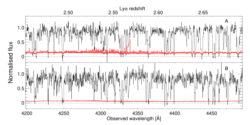
Figure S13: Spectra from the pair sample as in Fig. 1 of the main text, but for SDSS J000450.90-084452.0 (panel A) and SDSS J000450.66-084449.6 (panel B).

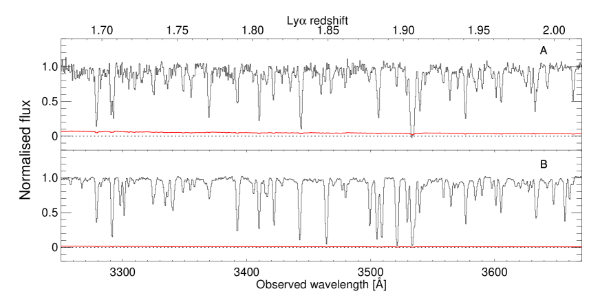
Figure S14: Spectra from the pair sample as in Fig. 1 of the main text, but for SDSS J005408.47-094638.3 (panel A) and SDSS J005408.04-094625.7 (panel B).

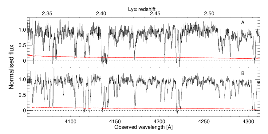
Figure S15: Spectra from the pair sample as in Fig. 1 of the main text, but for SDSS J011707.52+315341.2 (panel A) and SDSS J011708.39+315338.7 (panel B).

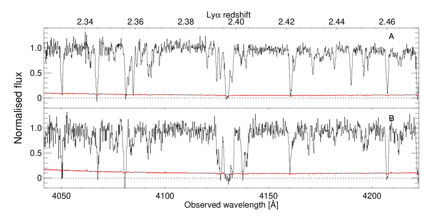
Figure S16: Spectra from the pair sample as in Fig. 1 of the main text, but for SDSS J025049.09-025631.7 (panel A) and SDSS J025048.86-025640.7 (panel B).

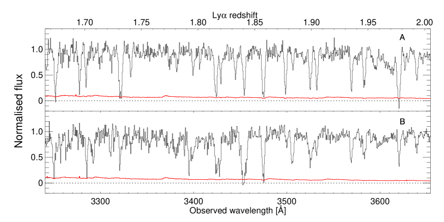
Figure S17: Spectra from the pair sample as in Fig. 1 of the main text, but for SDSS J033237.19-072219.6 (panel A) and SDSS J033238.38-072215.9 (panel B).

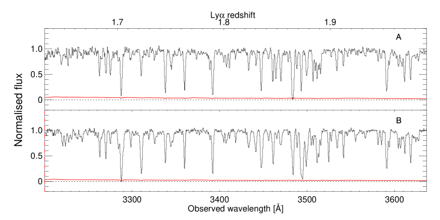
Figure S18: Spectra from the pair sample as in Fig. 1 of the main text, but for SDSS J073522.43+295710.1 (panel A) and SDSS J073522.55+295705.0 (panel B).

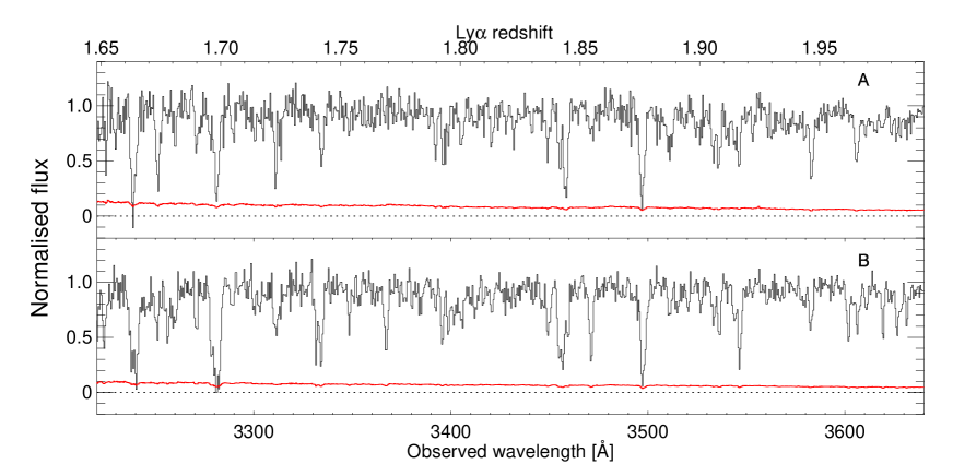
Figure S19: Spectra from the pair sample as in Fig. 1 of the main text, but for SDSS J081329.49+101405.2 (panel A) and SDSS J081329.71+101411.6 (panel B).

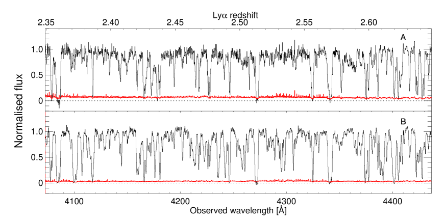
Figure S20: Spectra from the pair sample as in Fig. 1 of the main text, but for SDSS J091338.97-010704.6 (panel A) and SDSS J091338.30-010708.7 (panel B).

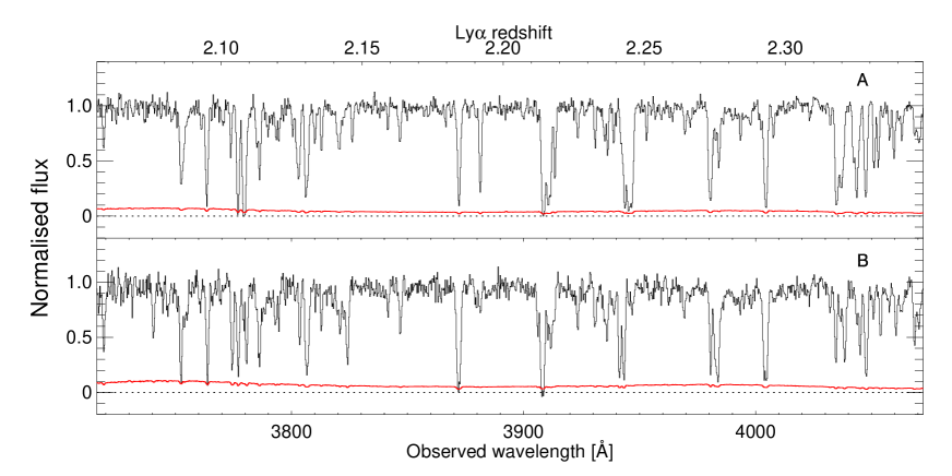
Figure S21: Spectra from the pair sample as in Fig. 1 of the main text, but for SDSS J092056.24+131057.4 (panel A) and SDSS J092056.01+131102.7 (panel B).

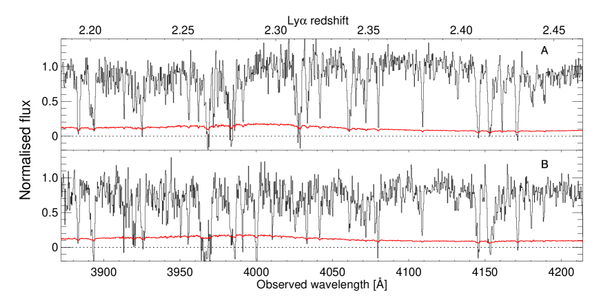
Figure S22: Spectra from the pair sample as in Fig. 1 of the main text, but for SDSS J093747.24+150928.0 (panel A) and SDSS J093747.40+150939.5 (panel B).

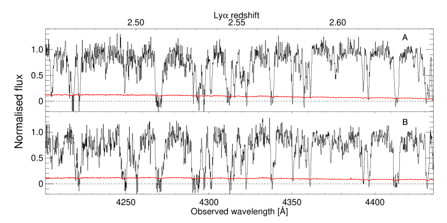
Figure S23: Spectra from the pair sample as in Fig. 1 of the main text, but for SDSS J093959.41+184757.1 (panel A) and SDSS J093959.02+184801.8 (panel B).

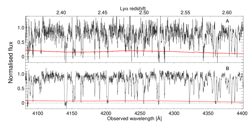
Figure S24: Spectra from the pair sample as in Fig. 1 of the main text, but for SDSS J101201.68+311348.6 (panel A) and SDSS J101201.77+311353.9 (panel B).

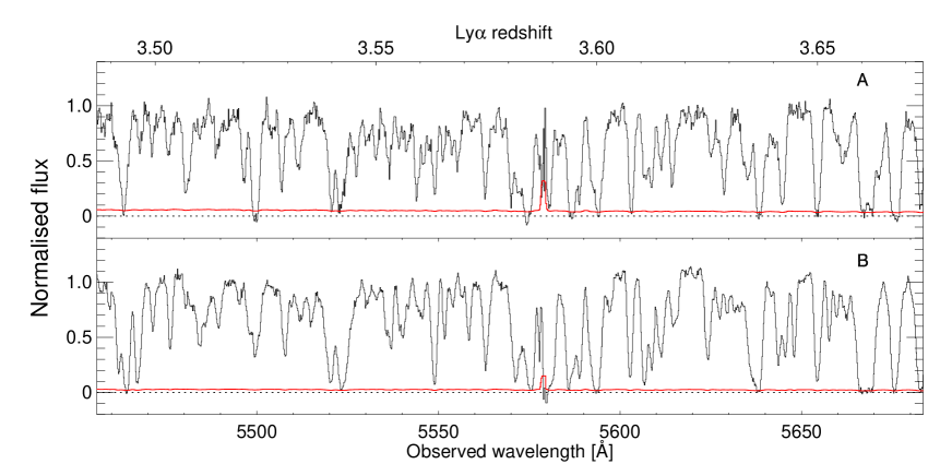
Figure S25: Spectra from the pair sample as in Fig. 1 of the main text, but for SDSS J102116.98+111227.6 (panel A) and SDSS J102116.47+111227.8 (panel B).

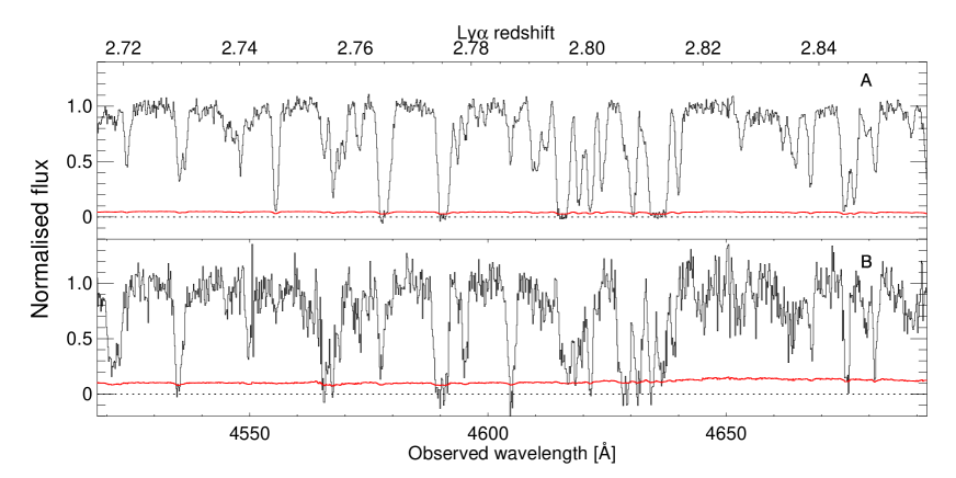
Figure S26: Spectra from the pair sample as in Fig. 1 of the main text, but for SDSS J111610.69+411814.4 (panel A) and SDSS J111611.74+411821.5 (panel B).

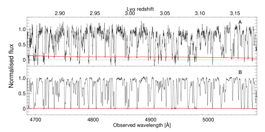
Figure S27: Spectra from the pair sample as in Fig. 1 of the main text, but for SDSS J114958.26+430041.3 (panel A) and SDSS J114958.49+430048.4 (panel B).

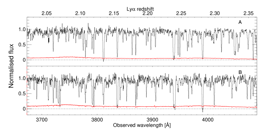
Figure S28: Spectra from the pair sample as in Fig. 1 of the main text, but for SDSS J120416.69+022111.0 (panel A) and SDSS J120417.47+022104.7 (panel B).

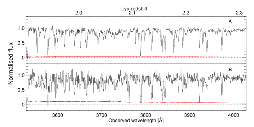
Figure S29: Spectra from the pair sample as in Fig. 1 of the main text, but for SDSS J122545.24+564445.1 (panel A) and SDSS J122545.73+564440.7 (panel B).

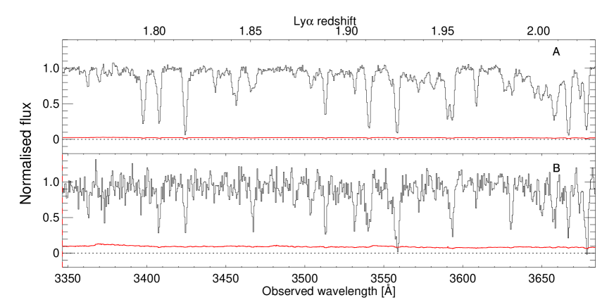
Figure S30: Spectra from the pair sample as in Fig. 1 of the main text, but for SDSS J140502.41+444754.4 (panel A) and SDSS J140501.94+444759.9 (panel B).

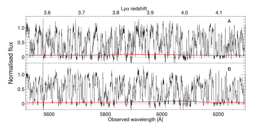
Figure S31: Spectra from the pair sample as in Fig. 1 of the main text, but for SDSS J142023.77+283106.6 (panel A) and SDSS J142023.80+283055.7 (panel B).

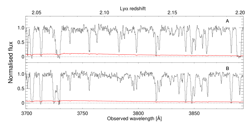
Figure S32: Spectra from the pair sample as in Fig. 1 of the main text, but for SDSS J142758.74-012136.2 (panel A) and SDSS J142758.89-012130.4 (panel B).

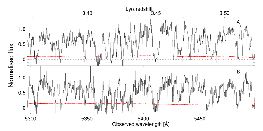
Figure S33: Spectra from the pair sample as in Fig. 1 of the main text, but for SDSS J154110.40+270231.2 (panel A) and SDSS J154110.37+270224.8 (panel B).

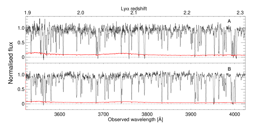
Figure S34: Spectra from the pair sample as in Fig. 1 of the main text, but for SDSS J161302.03+080814.3 (panel A) and SDSS J161301.69+080806.1 (panel B).

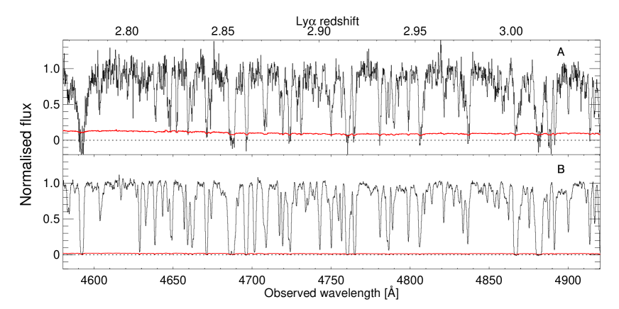
Figure S35: Spectra from the pair sample as in Fig. 1 of the main text, but for SDSS J162210.11+070215.3 (panel A) and SDSS J162209.81+070211.5 (panel B).

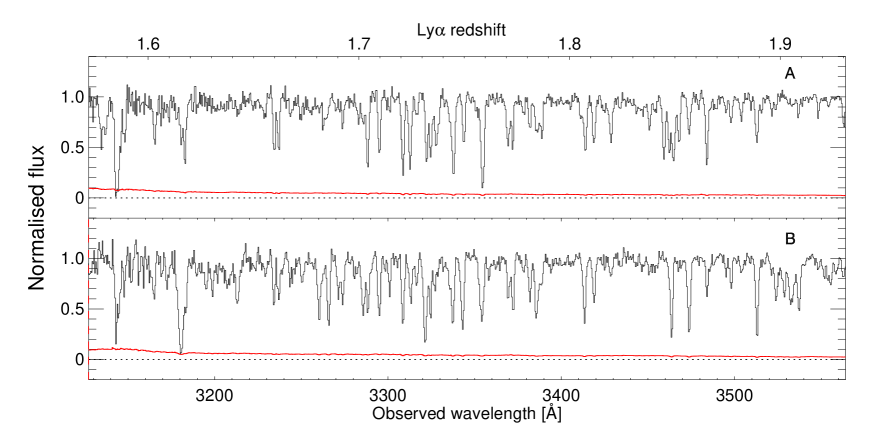
Figure S36: Spectra from the pair sample as in Fig. 1 of the main text, but for SDSS J221427.03+132657.0 (panel A) and SDSS J221426.79+132652.3 (panel B).

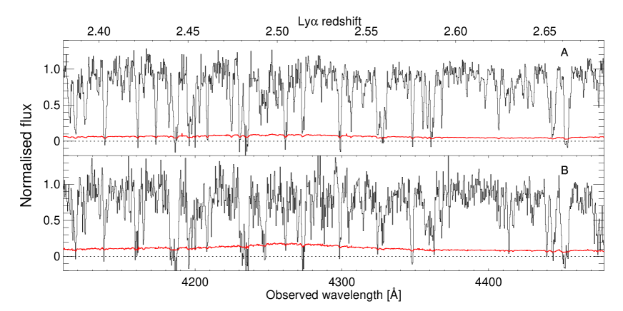
Figure S37: Spectra from the pair sample as in Fig. 1 of the main text, but for SDSS J230044.52+015552.1 (panel A) and SDSS J230044.36+015541.7 (panel B).

Acknowledgements
We thank Kate Rubin, Marie Lau, George Djorgovski, Crystal Martin, Sara Ellison and Rob Simcoe for helping with data collection and reduction.

We thank G. Becker, M. Haehnelt, and the ENIGMA group (http:// enigma.physics.ucsb.edu) for useful discussion and comments on early versions of this work. Some of the archival data used in this paper were collected and/or reduced by M. Fumagalli, K. Rubin, M. Lau, G. Djorgovski, C. Martin, S. Ellison, and R. Simcoe. Supported by the Alexander von Humboldt Foundation and the Max Planck Society (J.F.H.), NSF grant AST-1010004 (J.X.P.), U.S. Department of Energy (DOE) grant DE-AC02-05CH11231 (Z.L.), and European Research Council grant 320596 (G.K.). Calculations in this paper used resources of the U.S. National Energy Research Scientific Computing Center and of the Max Planck Computing and Data Facility supported by the Max Planck Society. Some data were obtained at the W. M. Keck Observatory, which is operated as a scientific partnership among the California Institute of Technology, the University of California, and NASA. The Observatory was made possible by the financial support of the W. M. Keck Foundation. We recognize and acknowledge the important cultural role and reverence that the summit of Mauna Kea has always had within the indigenous Hawaiian community; we are most fortunate to have the opportunity to conduct observations from this mountain. Some data were obtained with the 6.5-m Magellan Telescopes located at Las Campanas Observatory, Chile. Some data were obtained with the European Southern Observatory Very Large Telescope under programs 090.A-0824 and 089.A-0855. Spectra for all quasar pairs are shown in the supplementary materials. All the observational data analyzed in this paper are available in public archives. Simulation code and output files are also available in public repositories. Full details and URLs are provided in the supplementary materials.

References and Notes

- 1. A. A. Meiksin, Reviews of Modern Physics 81, 1405 (2009).
- 2. L. Hui, N. Y. Gnedin, MNRAS 292, 27 (1997).
- 3. N. Y. Gnedin, L. Hui, MNRAS 296, 44 (1998).
- 4. L. Hui, Z. Haiman, ApJ 596, 9 (2003).
- 5. G. Kulkarni, J. F. Hennawi, J. Oñorbe, A. Rorai, V. Springel, ApJ 812, 30 (2015).
- 6. J. A. Kollmeier, J. Miralda-Escudé, R. Cen, J. P. Ostriker, ApJ 638, 52 (2006).
- 7. V. Desjacques, M. G. Haehnelt, A. Nusser, MNRAS 367, L74 (2006).
- 8. M. Viel, J. Weller, M. G. Haehnelt, MNRAS 355, L23 (2004).
- 9. U. Seljak, A. Slosar, P. McDonald, J. Cosmology Astropart. Phys 10, 014 (2006).
- 10. M. McQuinn, P. R. Upton Sanderbeck, MNRAS 456, 47 (2016).
- 11. P. McDonald, et al., ApJ 543, 1 (2000).
- 12. M. Zaldarriaga, L. Hui, M. Tegmark, ApJ 557, 519 (2001).
- 13. R. A. C. Croft, et al., ApJ 581, 20 (2002).
- 14. M. S. Peeples, D. H. Weinberg, R. Davé, M. A. Fardal, N. Katz, MNRAS 404, 1281 (2010).
- 15. M. S. Peeples, D. H. Weinberg, R. Davé, M. A. Fardal, N. Katz, MNRAS 404, 1295 (2010).
- 16. A. Rorai, J. F. Hennawi, M. White, ApJ 775, 81 (2013).
- 17. E. Puchwein, et al., MNRAS 450, 4081 (2015).
- 18. J. Oñorbe, J. F. Hennawi, Z. Lukić, ArXiv e-prints (2016).
- 19. J. Schaye, ApJ 559, 507 (2001).
- 20. C. B. Foltz, R. J. Weymann, H.-J. Roser, J. F. H. Chaffee, ApJ 281, L1 (1984).
- 21. A. Smette, et al., ApJ 389, 39 (1992).
- 22. J. F. Hennawi, et al., AJ 131, 1 (2006).
- 23. J. F. Hennawi, et al., ApJ 719, 1672 (2010).
- 24. Materials and methods are available as supplementary materials on Science Online.
- 25. J. E. Gunn, B. A. Peterson, ApJ 142, 1633 (1965).
- 26. F. Haardt, P. Madau, ApJ 746, 125 (2012).
- 27. G. D. Becker, J. S. Bolton, M. G. Haehnelt, W. L. W. Sargent, MNRAS 410, 1096 (2011).
- 28. E. Boera, M. T. Murphy, G. D. Becker, J. S. Bolton, MNRAS 441, 1916 (2014).
- 29. A. Lidz, et al., ApJ 718, 199 (2010).
- 30. M. Viel, G. D. Becker, J. S. Bolton, M. G. Haehnelt, Phys. Rev. D 88, 043502 (2013).
- 31. L. Hui, J. P. Ostriker, S. Tremaine, E. Witten, ArXiv e-prints (2016).
- 32. J. R. Shaw, A. Lewis, Phys. Rev. D 86, 043510 (2012).
- 33. K. L. Pandey, S. K. Sethi, ApJ 762, 15 (2013).
- 34. S. Chongchitnan, A. Meiksin, MNRAS 437, 3639 (2014).
- 35. A. Meiksin, E. R. Tittley, MNRAS 423, 7 (2012).
- 36. J. S. Bolton, G. D. Becker, M. G. Haehnelt, M. Viel, MNRAS 438, 2499 (2014).
- 37. C.-A. Faucher-Giguère, J. X. Prochaska, A. Lidz, L. Hernquist, M. Zaldarriaga, ApJ 681, 831 (2008).
- 38. K. N. Abazajian, et al., ApJS 182, 543 (2009).
- 39. C. P. Ahn, et al., ApJS 203, 21 (2012).
- 40. S. M. Croom, et al., MNRAS 349, 1397 (2004).
- 41. J. Bovy, et al., ApJ 729, 141 (2011).
- 42. J. Bovy, et al., ApJ 749, 41 (2012).
- 43. M. A. DiPompeo, J. Bovy, A. D. Myers, D. Lang, MNRAS 452, 3124 (2015).
- 44. J. F. Hennawi, Topics in gravitational lensing: Clusters, quasars, and the cosmic microwave background, Ph.D. thesis, Ph.D dissertation, 2004. 232 pages; United States – New Jersey: Princeton University; 2004. Publication Number: AAT 3151085. DAI-B 65/10, p. 5189, Apr 2005 (2004).
- 45. J. B. Oke, et al., PASP 107, 375 (1995).
- 46. J. X. Prochaska, et al., ApJ 776, 136 (2013).
- 47. A. I. Sheinis, et al., PASP 114, 851 (2002).
- 48. C. L. Martin, et al., ApJ 721, 174 (2010).
- 49. S. L. Ellison, J. F. Hennawi, C. L. Martin, J. Sommer-Larsen, MNRAS 378, 801 (2007).
- 50. J. L. Marshall, et al., Ground-based and Airborne Instrumentation for Astronomy II (2008), vol. 7014 of Proc. SPIE, p. 701454.
- 51. J. Vernet, et al., A&A 536, A105 (2011).
- 52. K.-G. Lee, et al., ApJ 799, 196 (2015).
- 53. J. F. Hennawi, N. Dalal, P. Bode, ApJ 654, 93 (2007).
- 54. M. Rauch, W. L. W. Sargent, T. A. Barlow, R. F. Carswell, ApJ 562, 76 (2001).
- 55. J. F. Hennawi, J. X. Prochaska, ApJ 766, 58 (2013).
- 56. A. Dall’Aglio, L. Wisotzki, G. Worseck, A&A 491, 465 (2008).
- 57. J. M. O’Meara, et al., AJ 150, 111 (2015).
- 58. S. S. Vogt, et al., Instrumentation in Astronomy VIII, D. L. Crawford, E. R. Craine, eds. (1994), vol. 2198 of Proc. SPIE, p. 362.
- 59. N. Palanque-Delabrouille, et al., A&A 559, A85 (2013).
- 60. N. R. Lomb, Ap&SS 39, 447 (1976).
- 61. A. Mathias, et al., Journal of Statistical Software 11, 1 (2004).
- 62. R. Penrose, Mathematical Proceedings of the Cambridge Philosophical Society 51, 406 (1955).
- 63. R. A. C. Croft, D. H. Weinberg, N. Katz, L. Hernquist, ApJ 495, 44 (1998).
- 64. A. Meiksin, M. White, MNRAS 324, 141 (2001).
- 65. N. Y. Gnedin, et al., ApJ 583, 525 (2003).
- 66. M. White, ApJS 143, 241 (2002).
- 67. K. Heitmann, et al., Computational Science and Discovery 1, 015003 (2008).
- 68. Planck Collaboration, et al., A&A 571, A16 (2014).
- 69. J. Ribaudo, N. Lehner, J. C. Howk, ApJ 736, 42 (2011).
- 70. J. X. Prochaska, J. M. O’Meara, G. Worseck, ApJ 718, 392 (2010).
- 71. B. F. Lundgren, et al., ApJ 698, 819 (2009).
- 72. D. P. Schneider, et al., AJ 139, 2360 (2010).
- 73. I. Pâris, et al., A&A 548, A66 (2012).
- 74. A. J. Ross, et al., MNRAS 424, 564 (2012).
- 75. K. Heitmann, M. White, C. Wagner, S. Habib, D. Higdon, ApJ 715, 104 (2010).
- 76. K. Heitmann, et al., ApJ 705, 156 (2009).
- 77. E. Lawrence, et al., ApJ 713, 1322 (2010).
- 78. D. Foreman-Mackey, D. W. Hogg, D. Lang, J. Goodman, PASP 125, 306 (2013).
- 79. K. H. R. Rubin, et al., ApJ 808, 38 (2015).
- 80. M. Fumagalli, et al., ApJ 780, 74 (2014).
- 81. A. S. Almgren, J. B. Bell, M. J. Lijewski, Z. Lukić, E. Van Andel, ApJ 765, 39 (2013).
- 82. Z. Lukić, et al., MNRAS 446, 3697 (2015).
- 83. Planck Collaboration, et al., A&A 594, A13 (2016).
- 84. G. L. Bryan, M. E. Machacek, ApJ 534, 57 (2000).
- 85. E. Komatsu, et al., ApJS 192, 18 (2011).