An Expanded Chemo-dynamical Sample of Red Giants in the Bar of the Large Magellanic Cloud

Abstract

We report new spectroscopic observations obtained with the Michigan/Magellan Fiber System of 308 red giants (RGs) located in two fields near the photometric center of the bar of the Large Magellanic Cloud. This sample consists of 131 stars observed in previous studies (in one field) and 177 newly-observed stars (in the second field) selected specifically to more reliably establish the metallicity and age distributions of the bar. For each star, we measure its heliocentric line-of-sight velocity, surface gravity and metallicity from its high-resolution spectrum (effective temperatures come from photometric colors). The spectroscopic Hertzsprung-Russell diagrams—modulo small offsets in surface gravities—reveal good agreement with model isochrones. The mean metallicity of the 177-RG sample is $\rm[Fe/H]=-0.76\pm 0.02$ with a metallicity dispersion $\sigma=0.28\pm 0.03$. The corresponding metallicity distribution—corrected for selection effects—is well fitted by two Gaussian components: one metal-rich with a mean $-0.66\pm 0.02$ and a standard deviation $0.17\pm 0.01$, and the other metal-poor with $-1.20\pm 0.24$ and $0.41\pm 0.06$. The metal-rich and metal-poor populations contain approximately 85% and 15% of stars, respectively. We also confirm the velocity dispersion in the bar center decreases significantly from $31.2\pm 4.3$ to $18.7\pm 1.9$ km s^-1 with increasing metallicity over the range $-2.09$ to $-0.38$. Individual stellar masses are estimated using the spectroscopic surface gravities and the known luminosities. We find that lower mass hence older RGs have larger metallicity dispersion and lower mean metallicity than the higher-mass, younger RGs. The estimated masses, however, extend to implausibly low values ($\rm\sim 0.1~{}M_{\odot}$) making it impossible to obtain an absolute age-metallicity or age distribution of the bar.

1. Introduction

The Large Magellanic Cloud (LMC) is the nearest gas-rich satellite of the Milky Way that has ongoing star formation. The visual structure of the LMC is dominated by a prominent central bar, and hence we define the galaxies of this kind as Barred Magellanic Sprials (de Vaucouleurs & Freeman, 1972) or SB(s)m (de Vaucouleurs et al., 1991). Magellanic systems are common in the local universe, but they are rarely found as close to a massive parent system as the LMC to the Milky Way (Wilcots & Prescott, 2004; Liu et al., 2011; Tollerud et al., 2011; Robotham et al., 2012). Because of its relative proximity and prominence, the central bar of the LMC represents a particularly useful test case to explore how such structures develop and evolve in galactic systems.

It is well known that the LMC has a stellar bar that has no counterpart in the distribution of neutral or ionized gas (e.g., Kim et al., 1998; Bica et al., 1999; Staveley-Smith et al., 2003). More interestingly, the stellar bar is found to have multiple centers. The photometric center of the LMC bar, i.e. the densest point on a star count map, lies about 0.4 kpc away from the center of its stellar disk, and even more than 1 kpc away from the dynamical center of the neutral gas disk (van der Marel, 2001). The location of the stellar dynamical center is still under debate. According to the line-of-sight (LOS) kinematics, the dynamical center of the carbon stars is consistent with the photometric bar center (van der Marel et al., 2002; Olsen et al., 2011). In contrast, the average proper motion (PM) data observed by Hubble Space Telescope (HST) imply the stellar dynamical center coincides with the H i dynamical center (Kallivayalil et al., 2006; Piatek et al., 2008; Kallivayalil et al., 2013; van der Marel & Kallivayalil, 2014). When combining the LOS velocities and the PM data, van der Marel & Kallivayalil (2014) even found that the stellar dynamical center is intermediate between the photometric bar center and the H i dynamical center.

Kormendy & Kennicutt (2004) distinguish ‘true’ bars, which are formed in a quasi-independent manner early in the history of a disk galaxy, from ‘secular’ bars that develop over time from instabilities in disk galaxies. The off-center feature of the LMC bar strongly supports the secular evolution scenario resulting from tidal interactions. Many numerical simulations have been employed to reproduce the morphology and internal dynamics of the LMC including its off-center bar, but the detailed evolution remains uncertain. For example, Bekki (2009) showed that the off-center bar can be formed if the LMC with an already-existing bar can collide with a low-mass Galactic subhalo. Alternatively, more recent works prefer a dwarf-dwarf galaxy interaction (e.g., Besla et al., 2012; Yozin & Bekki, 2014; Pardy et al., 2016), presumably, in the case of the LMC, involving the Small Magellanic Cloud (SMC).

The star clusters in the LMC are rarely found to have ages between approximately 3 and 12 Gyr ago (e.g., Olszewski et al., 1996; Geisler et al., 1997), though this age interval appears to be filled by field stars (e.g., Holtzman et al., 1999; Smecker-Hane et al., 2002). This suggests either that the star formation associated with star clusters was suppressed during this ‘age gap’, or that clusters older than about 4 Gyr are preferentially destroyed (though not all; the LMC does contain a set of about ten ‘ancient’ star clusters comparable in age to globular clusters in the Galaxy). Whatever the cause for the age gap in the cluster population, the fact remains that if we aim to probe the history of the LMC for ages greater than about 4 Gyr, we must rely on field stars. Although many photometric studies have been carried out to do this (e.g., Smecker-Hane et al., 2002), interpretation is complicated by the increased insensitivity of the main-sequence turnoff with age, and the fact that all evolved stars older than about 1 Gyr essentially funnel into a single red-giant branch for a given metallicity (Bressan et al., 2012). In the LMC bar, crowding introduces an additional complication for ground-based studies, while HST observations tend to have limited field coverage. Spectroscopic studies of the LMC bar can be used as as a tool to determine the age-metallicity relation of the bar and to explore the star formation history of this enigmatic component of the LMC.

Many spectroscopic studies in the LMC bar and/or inner disk has been carried out during the past two decades. Gratton et al. (2004) analyzed low resolution spectroscopy of 98 RR Lyrae stars in the LMC bar, and reported an average metallicity of $-1.48$ dex for this old population. Cole et al. (2005, hereafter ‘C05’) carried out the first spectroscopic study of intermediate-age and old field stars in the LMC bar. The spectra of 373 red giants (RGs) were obtained at the near-infrared Ca ii triplet (CaT) and used to derive radial velocities and metallicities. They found a metallicity distribution function (MDF) peaked at $\rm[Fe/H]=-0.40$ dex with a tail of metal-poor stars down to $\rm[Fe/H]\leq-2.1$ dex and a systemic change in velocity dispersion with mean chemical abundance. Carrera et al. (2011) reanalyzed C05’s spectra and also obtained an average metallicity of $-0.40$ dex with a new calibration. On the other hand, studies on the inner disk reported lower mean metallicities than that of C05. Carrera et al. (2008) derived $\rm[Fe/H]\approx-0.5$ dex for a field about $3^{\circ}$ north of the LMC bar at first, and then Carrera et al. (2011) recalibrated a new mean of $-0.58$ dex for the same field. Lapenna et al. (2012) derived $\rm[Fe/H]=-0.48$ dex from 89 stars located about $2^{\circ}$ NW from the center of the LMC. More recently, Van der Swaelmen et al. (2013, hereafter ‘VdS13’) performed a detailed chemical analysis of 106 RGs in the sample of C05, using spectra obtained with the FLAMES/GIRAFFE multifibre spectrograph. Their measurements confirmed that C05 had overestimated the metallicities of metal-rich stars (by $0.25\pm 0.03$ dex from our calculation). Unfortunately, a reliable MDF of the LMC bar cannot be derived from their results due to inherent metallicity-dependent biases in their sample.

Since the nature of LMC bar remains poorly constrained in terms of the galaxy’s interaction and chemical evolution history, we aim to expand previous spectroscopic studies by observing a new sample of stars chosen using well-defined selection criteria. The ultimate aim is to produce a spectroscopic survey of evolved stars that can be used to map the chemo-dynamical properties as a function of position and age over the entire LMC bar region. In addition to 131 RGs observed by C05, our sample contains 177 more RGs selected from the OGLE-II photometry database (Udalski et al., 1997, 2000; Szymanski, 2005) for fully providing the bar MDF. The spectra were obtained with the Michigan/Magellan Fiber System (M2FS, Mateo et al., 2012) over two separate fields that both are near the photometric center of the LMC bar. This paper represents a first look at the results of this survey and provides a description of the techniques we employ.

The structure of the paper is as follows. Section 2 introduces the sample selection, the observations and the data reduction processes. Section 3 explains the measurements of velocities and stellar parameters that we derive from our spectra. Section 4 reports the main results of this work and describes some of their implications. In Section 5, we summarize and further discuss the key results of this study. We close with a cautionary tale regarding the inherent and still significant complications in using field stars to independently probe the age distribution/star-formation history in an intermediate-age/old population such as the LMC bar.

2. Observations and Data Reduction

2.1. Fields and Target Selection

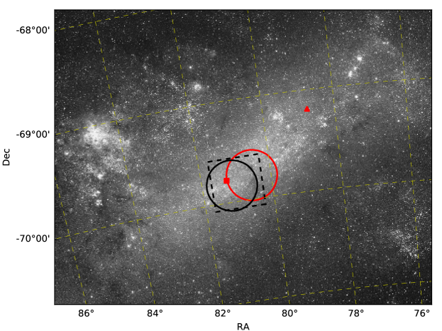
In standard operation, M2FS fields must be centered on a relatively bright ‘Shack-Hartmann’ (SH) star, which provides low-frequency wavefront data to the active optics system of the Magellan/Clay Telescope. Two additional spatially-coherent fiber bundles are used to image a pair of guide stars during exposures. Finally, a set of bright acquisition stars imaged through science fibers and visible on the guide camera are used for each field to held centroid the fibers in the field in both translation and rotation. These requirements ancillary stars impose mild restrictions on any M2FS field locations, but especially in crowded regions like the LMC bar. The data obtained for this study were collected in two bar fields labelled as ‘LMCC’ and ‘LMC1’, respectively. The trailing letter of ‘LMCC’ stands for ‘Cole’ because this field was chosen to include as many stars as practical from the sample of C05. The centers of these fields are listed in Table 1, and their locations and coverage areas are shown in Figure 1 along with the photometric bar center and the dynamical center constrained by stellar proper motions (van der Marel & Kallivayalil, 2014).

We used two different methods to select the stellar candidates in the LMCC and LMC1 fields. In LMCC, the candidate RGs were directly selected from the sample of C05 by first ranking their stars by metallicity and then selecting every other one to produce a suitably-sized subsample for M2FS followup. In LMC1, the candidate RGs were randomly selected from the OGLE-II $BVI$ maps of the LMC (Udalski et al., 2000), according to the following photometric criteria:

$$16.00<I<17.00,\ 22.00<I+5\times(V-I)<24.25.$$ (1)

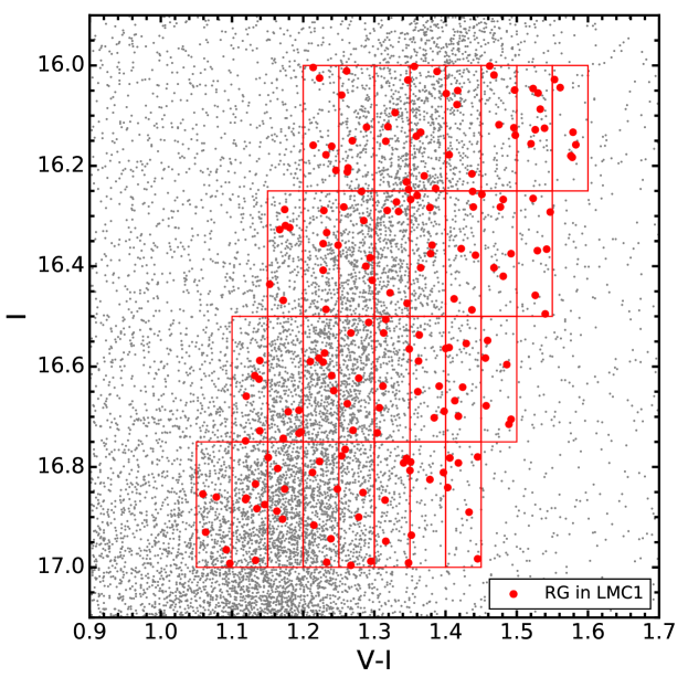
These limits were chosen to sample fully the color range–and hence the evidently wide metallicity range–of the population. As shown in Figure 3, we further divided the selection region into 32 rectangles and selected 6 candidates from each. This approach ensures that we sampled stars over a full color/metallicity/age range as populated within the red giant branch and allows us to account for selection when we generate the underlying metallicity distribution in the bar (see Section 4.2).

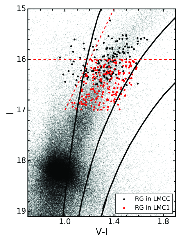
As already intimated, the operational characteristics of M2FS affect the selection process. M2FS employs aluminum fiber plugplates to position up to 256 optical fibers at the Nasmyth-East focal surface of the Magellan/Clay Telescope. Each fiber has an entrance aperture of 1.2 arcsec and is fitted in a ferrule 13 arcsec in diameter; the latter defines the minimum separation between deployed fibers. Otherwise, any fiber can be positioned anywhere within a field of 29 arcmin in diameter except at locations for various ancillary stars used for guiding, field alignment/acquisition, and active optical control (the central SH star noted above). In the end, we were able to assign 147 science fibers in the LMCC field, and 184 science fibers in LMC1. Table 2 lists the positions and photometric information of the observed stars. We also plot the locations of both LMCC and LMC1 samples on the color-magnitude diagram (CMD) in Figure 2.

2.2. Spectroscopic Observations

The summary of our LMC bar observations is listed in Table 1 including the total exposure time for each field. M2FS employs twin spectrographs (which are referred to as ‘blue’ and ‘red’ channels, respectively) that have identical optical properties and wavelength coverage but can be operated independently in a variety of spectral configurations. In our LMCC and LMC1 observations, both spectrographs were configured to sample a wavelength range of 5130–5189 Åat an effective resolution $\mathcal{R}\sim 20,000$. Each spectrograph images the raw spectra onto a four-channel $4096\times 4112$ E2V CCD with a pixel size of $\rm 15~{}\mu m$. During the readout process, we binned the data by $2\times 2$, which still over-samples the data in both spectral and spatial directions. The CCDs were readout in ‘slow’ mode for a typical gain of 0.75 e^-/ADU and a readout noise of 2.7 e^-.

Immediately before or after science exposures, we acquired calibration frames from a Th-Ar arc lamp (for wavelength calibration) and a quartz lamp (for spectral tracing). In addition, several twilight frames (which also included arc and quartz exposures) were obtained at either the beginning or the end of the same observing night. These twilight data are used to check the wavelength/velocity calibration and correct fiber-to-fiber throughput variations (Section 2.3), and also to estimate systematic offsets in the best-fit physical parameters (Section 3.3). We also obtained a master ‘fiber map’ with all the fibers plugged in while the telescope focal surface is illuminated by ambient daylight in the mostly-closed dome. The map produces a high signal-to-noise template for tracing spectra, and is useful as a parallel check on the relative fiber throughputs estimated from the twilights. Groups of bias (zero) and dark frames (also by $2\times 2$ binning) were also obtained during each observing run and combined to produce master bias and dark frames that are used in the data reduction.

Background subtraction is very important in this work because of the crowded LMC bar region. The central surface brightness of the LMC bar (see the red filled square in Figure 1) is $20.65\ \rm mag/arcsec^{2}$ in $V$-band (Bothun & Thompson, 1988). In contrast, the $V$-band telluric sky background would have ranged from about 22.0 (Dec 2014) to 21.6 (Nov 2015) $\rm mag/arcsec^{2}$ at the location of the LMC bar—about 3.5–2.4 times fainter than the LMC contribution—at the time of our observations.

We have therefore adopted two distinct approaches to obtain the background spectra in the LMCC and LMC1 fields, respectively. In LMCC, 95 sky-background fibers were assigned in addition to the 147 science fibers, and their positions were selected on the image obtained by STScI DSS. For selecting good background positions, we first randomly picked a position within the LMCC field and kept it if meeting two conditions: (a) the chosen position is well separated ($>13$ arcsec) from all other assigned fiber positions, and (b) the mean count of all pixels within a $5$ square centered on that position is within 10% of the modal background value of the image. In LMC1, no sky fibers were assigned in advance due to the initial use of these data for more limited M2FS commissioning purposes. To estimate the background contribution, we pointed the telescope 15 arcsec away from the original position—known as ‘off-target’ exposures—along three principal directions (North, South and East) during the Nov 2015 observation run. As a result, the background subtraction approaches differ slightly for the LMCC and LMC1 samples; we describe these in the following section.

2.3. Data Reduction

Condensed descriptions of standard M2FS data reduction processes can be found in Walker et al. (2015b, a). All data processing was carried out using IRAF scripts and pipelines designed for M2FS data, and the typical final products are background-subtracted stellar spectra.

Briefly, all data were first processed through overscan subtraction, bias correction and dark correction. We removed cosmic rays from almost all exposures (excluding arcs or other short exposures) using the Laplacian-filtering algorithm from van Dokkum (2001). We subtracted diffuse scattered light from the two-dimensional images by fitting a polynomial surface to the regions of the images not illuminated by the fibers. The spectral traces, defined by combining twilights/quartzes/fiber maps, were shifted to match the locations of the science spectra (named because they are extracted from the science exposures) that produced final science traces. The final science traces were used to extract the calibration arcs to ensure no offset or interpolation shift existing between the arc exposures and the science exposures. The extracted arcs were then fit to a moderate-order polynomial to determine the transformation from extracted-pixel to wavelength for every science fiber/target. The typical root-mean-square of these fits for the data used in this study was 0.3 km s^-1. The wavelength-calibrated data were then normalized using relative fiber throughputs derived from the twilights or fiber maps. For all the above steps, we processed the sky-background data—both from the sky-background fibers in LMCC and from the off-target exposures in LMC1—the same as the science data. Throughout the entire reduction process, we also calculated ‘variance spectra’ in order to track the signal-to-noise ratio (SNR) for every pixel of every science spectrum. These data are used to properly weight individual pixels when fitting spectra to model atmospheres in order to derive stellar parameters (see Section 3.1).

The last but important step is the background subtraction. In LMCC, we found no significant flux or spectral variations among sky-background fibers. We therefore averaged all these background spectra to make a master background spectrum and subtracted it directly from all science spectra. In LMC1, the background spectra were obtained from the off-target exposures one year later. After removing some anomalously high-flux spectra (about 10% of the total), we averaged all other spectra to made a second-year master background spectrum. Then this spectrum was scaled by a factor 1.8 before being subtracted from the deeper first-year science spectra. This factor accounts for differences in exposure times, atmospheric extinction, telluric background and seeing between the two sets of observations. The systematic reliability of this approach is confirmed in Section 4.2 where we demonstrate good agreement in the metallicity scales obtained independently from the M2FS data in the LMCC and LMC1 fields.

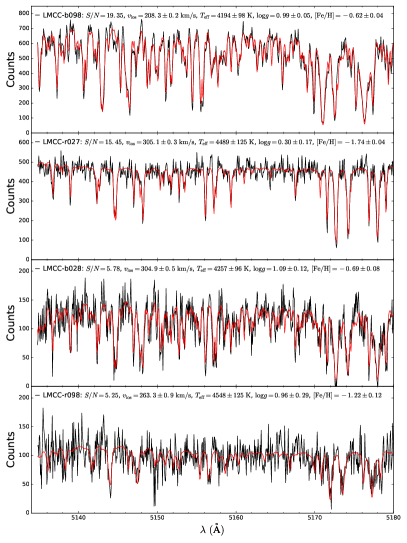
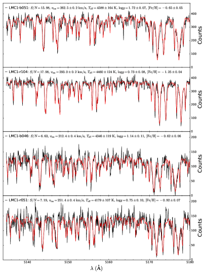
Figure 4 shows examples of background-subtracted spectra in the LMCC and LMC1 fields. The spectra span a range from the highest to lowest SNRs for our targets, and also a range in metallicities (measured through the method introduced in the following section).

3. Analysis

3.1. Modeling of M2FS Spectra

To measure the LOS velocity and the stellar parameters, we employ a Bayesian method to fit the background-subtracted M2FS spectrum (see Walker et al. (2015b, a)). For each star, this approach generates a model spectrum $M(\lambda)$ by combining a continuum-normalized template spectrum $T(\lambda)$ and an assumed continuum spectrum $P_{l}(\lambda)$,

$$M(\lambda)=P_{l}(\lambda)T(\lambda),$$ (2)

where $P_{l}(\lambda)$ is an $l$-order polynomial. This model spectrum $M(\lambda)$ is used to compare with the observed spectrum using a maximum-likelihood technique.

The template spectrum, $T(\lambda)$, is generated using a library of synthetic spectra, which is used in the Sloan Extension for Galactic Exploration and Understanding (SEGUE) stellar Parameter Pipeline (SSPP, Lee et al., 2008a, b). This library contains a set of rest-frame, continuum-normalized, stellar spectra, which are computed over a grid containing three atmospheric parameters, i.e. the effective temperature ($T_{\rm eff}$), the surface gravity ($\log{g}$, where $g$ is in $\rm cm\,s^{-2}$) and the metallicity ($\rm[Fe/H]$). These parameters vary in the following ranges (with the grid steps):

$$4000\leq T_{\rm eff} \leq 10000\ {\rm K},{\rm with}\ \Delta T_{\rm eff}=250\ {\rm K},$$

$$0\leq \log{g} \leq 5~{}{\rm dex},\ {\rm with}\ \Delta\log{g}=0.25\ {\rm dex},$$ (3)

$$-5\leq {\rm[Fe/H]} \leq 1~{}{\rm dex},\ {\rm with}\ \Delta{\rm[Fe/H]}=0.25\ {\rm dex},$$

For the $\alpha$ elements, their total abundance is typically fixed based on the iron abundance via the ratio $\rm[\alpha/Fe]$. This library assumes a hard-wired relation between $\rm[\alpha/Fe]$ and $\rm[Fe/H]$:

$${\rm[\alpha/Fe]}=\begin{cases}0.4&\text{for }{\rm[Fe/H]}<-1,\\ -0.4\times{\rm[Fe/H]}&\text{for }{\rm[Fe/H]}\in\left[-1,\,0\right],\\ 0&\text{for }{\rm[Fe/H]}\geq 0.\end{cases}$$ (4)

Another consideration is the wavelength shift between the template spectrum and the observed spectrum. This shift has two potential origins: the velocity shift due to the LOS velocity and the uncertainty of the wavelength solution in the observed spectrum. The first offset is accounted for by a parameter that shifts the wavelength as $\lambda^{\prime}=\lambda v_{\rm los}/c$, where $v_{\rm los}$ is the LOS velocity and $c$ is the speed of light. The wavelength solution may have residual systematic deviations, which could be modeled as a polynomial $Q_{m}(\lambda)$ of order $m$. Combining these two effects, the final shifted wavelength is

$$\lambda^{\prime}=\lambda\left[1+\frac{Q_{m}(\lambda)+v_{\rm los}}{c}\right],$$ (5)

and so the final template spectrum is now represented as $T(\lambda^{\prime})$.

To carry out the maximum-likelihood technique, we adopt the likelihood function used by Walker et al. (2015b),

$$\mathcal{L}(S(\lambda)|\vec{\theta},\,s_{1},\,s_{2})=$$

$$\prod_{i=1}^{N_{\lambda}}\frac{1}{\sqrt{2\pi(s_{1}{\rm Var}[S(\lambda_{i})]+s_{2}^{2})}}\exp\left[-\frac{1}{2}\frac{\left(S(\lambda_{i})-M(\lambda_{i})\right)^{2}}{s_{1}{\rm Var}[S(\lambda_{i})]+s_{2}^{2}}\right],$$

where $S(\lambda_{i})$ and $M(\lambda_{i})$ are the observed spectrum and the model spectrum, respectively, and $\vec{\theta}$ is a vector of all free parameters in $M(\lambda_{i})$ (summarized in the following paragraph). There are also two nuisance parameters $s_{1}$ and $s_{2}$ that, respectively, rescale and add an offset to the observational variances to account for systematically misestimated noises.

In practice, $P_{l}(\lambda)$ is treated as a fifth order polynomial (i.e., $l=5$) incorporating six parameters. The wavelength-shifted $T(\lambda^{\prime})$ inherits three parameters from the library spectra and three coefficients related to the modification of $Q_{m}(\lambda)$ (i.e., $m=2$). An additional parameter is varied to convolve the template spectra with the instrumental line-spread function (LSF), and thus $\vec{\theta}$ ends up with 13 free parameters. Considering the two nuisance parameters $s_{1}$ and $s_{2}$ in Eq. 3.1, the full fitting method contains 15 free parameters in the end, among which four of them are the physical parameters we aim to measure: $v_{\rm los}$, $T_{\rm eff}$, $\log{g}$ and $\rm[Fe/H]$. In each fitting, we truncate the spectrum in the region $5130\leq\lambda/$Å$\leq 5180$, while for the template spectra, the rest-frame wavelength region $5120\leq\lambda/$Å$\leq 5190$ are adopted to account for the LOS velocities up to about $\pm 550\rm\ km\ s^{-1}$.

3.2. Priors of the Physical Parameters

We use the MultiNest package (Feroz & Hobson, 2008; Feroz et al., 2009, 2013) to scan the parameter space. MultiNest implements a nested-sampling Monte Carlo algorithm, and returns random samplings from the posterior probability distribution functions (PDFs) for all input parameters. We record the first four moments of each physical parameter’s posterior PDF: mean, variance, skewness and kurtosis.

MultiNest requests a set of prior distributions for all parameters to initiate the calculation. We adopted uniform priors over a specified range of values as listed in Table 2 of Walker et al. (2015b). For the physical parameters $v_{\rm los}$, $\log{g}$ and ${\rm[Fe/H]}$, the priors were set within the ranges:

$$-500\leq v_{\rm los}/({\rm km\ s^{-1}})\leq 500,$$

$$0\leq\log{[g/({\rm cm\ s^{-2}})]}\leq 5,$$ (7)

$$-5\leq{\rm[Fe/H]}/{\rm dex}\leq 1.$$

Different from Walker et al. (2015b), $T_{\rm eff}$ was fixed during the fitting process in this study, because it proved difficult to constrain the temperatures adequately given the narrow wavelength range of our spectra and the typically modest median SNR per pixel (ranging from 5 to around 25). In addition, we found that the best-fit values for $\log{g}$ and $\rm[Fe/H]$ were strongly correlated with $T_{\rm eff}$ when using uniform temperature priors. To break this degeneracy, we calculated effective temperatures for our targets from the OGLE-II $V-I$ color index using color-temperature relation for giants (Equation 1 of Ramírez & Meléndez, 2005). We adopted a single-extinction model of $E(V-I)=0.15\pm 0.07$ mag, which is equivalent to $E(B-V)\approx 0.11$ mag, $A_{V}\approx 0.34$ mag and $A_{I}\approx 0.20$ mag in the UBVRI photometric system. Since the color-temperature relation reported by Ramírez & Meléndez (2005) is a weak function of metallicity, we simply assumed $\rm[Fe/H]=-0.8$ dex, the mean value for our targets when we used the Bayesian method with $T_{\rm eff}$ as a free parameter.

3.3. Twilight Offsets and Errors

We also applied the Bayesian method described above to the twilight spectra obtained on the same night and in the same spectrograph configuration. Using the solar effective temperature $T_{\rm eff,\,\odot}=5778\ {\rm K}$ as the fixed temperature prior, we found that the parameters $v_{\rm los}$, $\log{g}$ and $\rm[Fe/H]$ fitted from those spectra deviate from the known solar values, $v_{\rm los,\,\odot}=0\ {\rm km\,s^{-1}}$, $\log_{10}{[g_{\odot}/(\rm cm\,s^{-2})]}=4.44$ dex and $\rm[Fe/H]_{\odot}=0$ dex. As discussed in Walker et al. (2015b, a), we attribute this to systematic mismatches between the model spectrum and the observed spectra. Without independent information regarding how such mismatches may vary with spectral type, we defined the offsets between the fitting and the true twilight parameters to be zero-point shifts. Table 3 lists the mean offsets and the standard deviations of all three fitting physical parameters in each field and each channel.

According to Table 3, we apply the twilight offsets in $\rm[Fe/H]$ to all results obtained from the Bayesian analysis of our science spectra. For $v_{\rm los}$ and $\log{g}$, we chose not to apply offsets to the data as the required offsets are either not statistically significant, or they have no significant implications for our final results. The total error budget for our derived stellar parameters include contributions from the variances of the twilight offsets, the variances of the posterior PDFs of $v_{\rm los}$, $\log{g}$ and $\rm[Fe/H]$, and—for $T_{\rm eff}$—the uncertainty of the color excess $\sigma[E(V-I)]=0.07$ mag.

A full table of the final results is available in machine-readable format online. The initial few lines of this table is provided in Table 4. We list only results for spectra with median SNR per pixel greater than 5 ($\rm SNR>5$), which results in 133 (out of 147 observed) targets in LMCC and 179 (out of 184) in LMC1. Excluding double/blended stars (see Section 4.1), the final LMCC and LMC1 sample sizes are 131 and 177, respectively. Heliocentric corrections has been applied to all velocity results and were calculated using appropriate PyAstronomy routines.

3.4. Metallicity from the Equivalent Widths

In order to examine the accuracy of the Bayesian analysis (BA), we compare our metallicities with those derived using the traditional spectroscopic analysis. For this purpose, we selected 11 LMCC stars (see Table 5) that not only have high-SNR spectra ($\rm SNR>10$) but also show significant differences in the measured metallicities between our work and VdS13 ($\rm|[FeI/H]_{VdS13}-[Fe/H]_{Bayesian}|>0.2$ dex).

We restrict the analysis to Fe i lines with accurate $\log gf$ values (grade “D$+$” or better, $\sigma<$ 0.22 dex, according to the NIST Atomic Spectra Database; Kramida et al. 2015), which leaves us with three lines that can be measured in our spectra (5150.84, 5166.28 and 5171.60 Å). Our approach is to measure equivalent widths (EWs) of these lines through a semi-automated routine that fits Voigt line profiles to continuum-normalized spectra. We inspect these fits and then modify them if the automated routine clearly fails to identify the continuum, which often occurs when the routine incorrectly includes neighboring absorption lines in the calculation of the continuum. The uncertainties in the EW values are $\approx$ 10%.

Before applying this EW method to our M2FS spectra, we first measure EWs of these lines in high-quality spectra of two metal-poor RG standard stars, Arcturus (Hinkle et al., 2000) and HD 175305 (Roederer et al., 2014). The metallicities derived for the two standard stars are in good agreement with previous work. For Arcturus, we derive [Fe/H] $=-$0.41 $\pm$ 0.11 dex, which agrees with the value [Fe/H] $=-$0.52 $\pm$ 0.04 dex derived by Ramírez & Allende Prieto (2011). For HD 175305, we derive [Fe/H] $=-$1.61 $\pm$ 0.34 dex, which agrees with the value [Fe/H] $=-$1.56 $\pm$ 0.15 dex derived by Roederer et al. (2014). This indicates that for high resolution and high SNR stellar spectra, our EW method is reliable, and the choice of lines has little effect on the derived metallicities.

As an additional test, we have also degraded the resolution and SNR of these spectra to match our typical M2FS spectra. After remeasuring the EWs, the derived [Fe/H] values for these two standard stars are found to be approximately 0.2 dex lower than when the high-quality spectra are used. The statistical uncertainties of the derived abundances, however, are quite large (about 0.4 dex), so we do not consider this to represent strong evidence of a systematic offset in [Fe/H] induced by the modest SNR of our spectra. Finally, we also applied the BA to degraded spectra of Arcturus and HD 175305. In each case, we obtain [Fe/H] results to within 0.2 dex of the ‘true’ values.

For these 11 selected stars, we use the newly measured EW values with the formerly measured $T_{\rm eff}$ and log g  (listed in Table 5) to derive the metallicity for each star. We adopt a constant microturbulence velocity parameter, $v_{t}=2.0\pm 0.4$ km s^-1, for each star because we lack any constraints on this parameter. We derive the metallicities using a recent version of the spectrum analysis code MOOG (Sneden, 1973; Sobeck et al., 2011). The calculations are repeated 250 times for each star, resampling the stellar parameters and EWs each time from normal distributions.

Table 5 lists the metallicities derived by our BA and EW methods, as well as those measured by VdS13 and C05. We calculated the weighted mean differences in the metallicities among those measurements as

$$\langle\rm[Fe/H]_{\rm BA}-[Fe/H]_{\rm EW}\rangle=0.07\pm 0.12~{}\rm dex,$$

$$\langle\rm[Fe/H]_{\rm V13}-[Fe/H]_{\rm EW}\rangle=0.22\pm 0.14~{}\rm dex,$$ (8)

$$\langle\rm[Fe/H]_{\rm C05}-[Fe/H]_{\rm EW}\rangle=0.25\pm 0.15~{}\rm dex.$$

At face value, this analysis favors the BA results, but there are important caveats. For example, the limited wavelength coverage provides few reliable Fe i lines for the EW analysis, so the statistical uncertainties are large (see Table 5). The relatively low SNR of the spectra may also mask the presence of other weak lines in the spectra leading to a systematically low misplacement of the continuum level. This interpretation is supported by the results of our test to rederive [Fe/H] from the degraded standard star spectra described above. Nonetheless, lacking a set of standard stars observed in the same conditions for calibration, we find no need for any additional corrections to the BA metallicities beyond the twilight offset described in Section 3.3. We shall therefore adopt the BA metallicities as listed in Table 4 throughout the rest of this paper.

3.5. Comparison with Previous Studies

As stated in Section 3.3, we have 133 RGs left in the LMCC sample that were selected from C05’s sample. Among them, 39 were also reobserved by VdS13. These stars provide an opportunity to compare the physical parameter measurements on a star-by-star basis. In Figure 5, we compare the LOS velocities and the stellar parameters measured from our M2FS spectra to those reported by C05 (top panels) and VdS13 (middle and bottom panels).

For the subsample of 133 stars, we measured a mean heliocentric LOS velocity of $262.9\pm 2.1$ km s^-1 and a corresponding velocity dispersion of $24.4\pm 1.6$ km s^-1, compared to $258.7\pm 2.4$ km s^-1 and $27.0\pm 1.7$ km s^-1 measured by C05 (Figure 5a). The median errors of the individual velocities are $0.4$ km s^-1 (this work) and $7.5$ km s^-1 (C05). There is a systematic offset of $4.2\pm 0.8$ km s^-1 in the velocity measurements between these two studies (in the sense M2FS$-$C05). Figure 5b illustrates that we typically measure lower metallicities than C05 did for stars in common. Excluding the two anomalous sources in the upper-left corner of Figure 5b (see Section 4.1), the remaining 131 stars reveal weighted mean metallicities of $-0.76\pm 0.03$ dex (this work) and $-0.50\pm 0.03$ dex (C05). The corresponding metallicity dispersions are $0.30\pm 0.03$ dex and $0.37\pm 0.04$ dex, respectively. Although the dispersions are statistically equivalent, the systematic metallicity offset of $0.27\pm 0.04$ dex between our work and C05 appears to be significant.

For the subsample of 39 stars, we measured a mean heliocentric LOS velocity of $263.9\pm 3.6$ km s^-1, which is slightly greater than $262.4\pm 3.6$ km s^-1 by VdS13 and $258.9\pm 3.9$ km s^-1 by C05 (Figure 5c). The velocity dispersion is $22.0\pm 2.4$ km s^-1 from our measurements, compared to $22.1\pm 2.5$ km s^-1 (VdS13) and $24.3\pm 2.7$ km s^-1 (C05). The median errors in the single-star velocities are $0.3$ km s^-1 (our work), $0.2$ km s^-1 (VdS13), and $7.5$ km s^-1 (C05). The systematic offset between our velocities and VdS13 is $1.5\pm 0.2$ km s^-1 (in the sense M2FS$-$VdS13).

For the same 39 stars, we measured a mean metallicity value of [Fe/H] $=-0.80\pm 0.05$ dex, compared to $-0.71\pm 0.06$ dex from VdS13, and $-0.56\pm 0.06$ dex from C05. Given the median errors on metallicity in three studies are $0.06$ dex (this work), $0.12$ dex (VdS13) and $0.13$ dex (C05), we confirm that C05 seems to have overestimated the metallicity for metal-rich stars in the LMC bar by around $0.25$ dex. There is less evidence that such an offset exists among more metal-poor stars ($\rm[Fe/H]<-1.0$ dex) (Pompéia et al. 2008; VdS13), though the number of such stars we can directly compare from the various studies is not large. In contrast, our metallicity measurements are in statistically good agreement with those of VdS13.

Finally, we also compared $T_{\rm eff}$ and log g between our work and VdS13 in Figures 5e and 5f, respectively. Although VdS13 and we used different color-$T_{\rm eff}$ relations to calculate $T_{\rm eff}$ from photometry, the results of $T_{\rm eff}$ are in reasonably good agreement. The comparison of log g shows more scatter with no clear pattern. Note that VdS13 calculated their log g from photometry (see Section 5.1), while our log g are measured by comparing the scientific spectra to a library of templates. Our results imply poor agreement between these methods, which is an important conclusion for our aim to measure the age distribution function of LMC bar stars directly (Section 5.1).

4. Results

4.1. Spectroscopic Hertzsprung-Russell Diagram

It is well known from stellar evolutionary models (e.g., Girardi et al., 2000; Bressan et al., 2012) and observations of star clusters (e.g., Mermilliod, 1981; Meynet et al., 1993) that the classical red giant branch (RGB) in the Hertzsprung-Russell (HR) diagram typically consists of stars older than approximately 1 Gyr over a wide range of metallicities. The resulting age-metallicity degeneracy along the RGB stems from this evolutionary funneling effect (as it was called decades ago; e.g., Eggen, 1971), as well as the competing effects of age and metallicity on the photometric colors of such stars. From an astrophysical standpoint, this degeneracy makes it difficult to disentangle the age or metallicity distribution of an intermediate-age or old RG population from photometric observations. A key aim of this study is to use spectroscopy to try to break this degeneracy as far as possible by providing independent information on RGB metallicities and ages (via log g measurements).

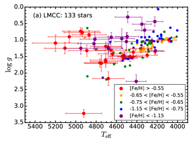
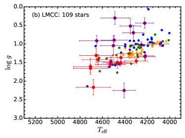
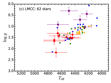
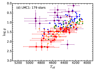
To illustrate the potential of this approach, we plot four spectroscopic HR diagrams showing the relationship between the stars’ surface gravities and their effective temperatures in Figure 6. On each diagram, the stars are color-coded by the same metallicity bins shown in the legend of Figure 6a. The first three diagrams (Figures 6a, 6b and 6c) are made to illustrate the complications in interpreting the LMCC sample. We reduce the LMCC sample size from 133 (in Figure 6a) to 62 (in Figure 6c) for the purpose of investigating the ‘peculiar’ metal-rich stars shown in the upper-left corner of Figure 6a. No such star has been found in the LMC1 sample and Figure 6d shows a clear segregation by metallicity.

At a first glance, the metal-dependent pattern in Figure 6d is very similar to that shown on the CMD of C05 (see their Figure 8). However, there is a significant difference between those two diagrams. In Figure 6d, the color-coded populations can be well separated by metallicity, with the extremely metal-poor stars located on the upper-left corner and the extremely metal-rich ones on the lower-right. On the other hand, the extremely metal-poor stars on C05’s CMD were overlapped by many relatively metal-rich counterparts, since the bluest stars in their sample are mostly metal-rich and a board color range is covered by the stars with metallicity around the peak of their MDF ($\rm-0.6<[Fe/H]<-0.3~{}dex$).

As described in Section 2.1, the stars in our LMCC sample were selected exclusively from C05’s sample. Their selection criteria on the CMD (also reflected by the large black dots in Figure 2) were chosen to include stars over a wide range of metallicity expected in the LMC bar. However, the blue edge of their selection region—chosen to include metal-poor RGs—is likely contaminated by metal-rich stars younger than about 1 Gyr, which arise either from the bar itself or from a superimposed disk population in the central region of the LMC (see the isochrones in Figure 2 as an example). Such stars show up clearly in Figure 6a, populating in the region of high $T_{\rm eff}$ and low $\log{g}$ (i.e. upper-left corner of the plot).

When imposing the same blue color cut as we did for LMC1 (i.e. $I+5\times(V-I)>22.00$ according to Eq. 1 and also see the tilt red dashed line in Figure 2), we exclusively remove these more massive giants, resulting in a sample of 109 stars shown in Figure 6b. Though a few old metal-poor stars are removed in this selection, the resulting HRD cannot be distinguished from that of the LMC1 sample (Figure 6d). C05’s sample also extends to a higher luminosity than our LMC1 sample (see the horizontal red dashed line in Figure 2). So we select another subsample from the LMCC sample using the same limits for the LMC1 sample (Eq. 1). The remaining 62 stars in Figure 6c produce an HRD in good agreement with the HRD of the full LMC1 sample shown in Figure 6d.

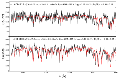
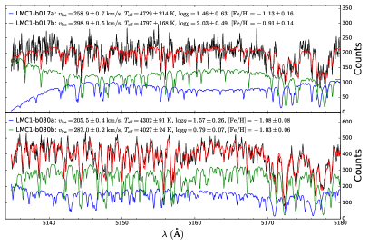
We note that a few apparently very metal-poor stars are located in the lower-right corner of both Figures 6b and 6d, where we would expect the most metal-rich giants. In the nomenclature of Table 4, their IDs are LMCC-b086, LMCC-r001, LMC1-b017 and LMC1-b080. On close inspection, we found that the spectra of LMC1-b017 and LMC1-b080 can be well fitted with a two-star rather than a single-star model. In Figure 7, their observed spectra are plotted on the left with their best-fit single-star model spectra. On the right, the best-fit spectra employing a two-star model is shown for comparison. For LMC1-b017, the reduced chi-square value decreases from 1.7 (single-star) to 1.0 (two-star); and for LMC1-b080, the reduced chi-square value decreases from 5.2 (single-star) to 2.0 (two-star). In both cases, the two-star fits are significantly better.

These two stars appear to be either spectroscopic binaries or physically unrelated stars that happen to be blended photometrically. We favor the second interpretation because double-RG binaries should be quite rare on stellar evolutionary timing grounds. For the two cases shown in Figure 7, the relative velocity shifts of the individual stars are in $40.0\pm 0.9$ km s^-1 for LMC1-b017 and $81.5\pm 0.4$ km s^-1 for LMC1-b080. Such velocities would be very difficult to explain in binary systems consisting of RGs with masses around 1 $\rm M_{\odot}$. Spectral blending—whether due to a physical or photometric binary—can also explain the inferred low metallicities of the stars. Since the stars have different systemic velocities, their lines will appear weaker relative to the approximately doubled continuum, resulting in a low inferred metallicity when fit as a single star. The other two anomalous stars in Figure 6b, i.e. LMCC-b086 and LMCC-r001, do not exhibit obviously composite spectra and it is unclear why they exhibit relatively high surface gravities for their low metallicities. Alternatively, these stars may be metal-poor subgiants located foreground to the LMC in the Galactic halo. Whatever the origin, we exclude these four stars from our RG sample and subsequent analysis. This resulting LMCC and LMC1 samples consist of 131 and 177 stars, respectively.

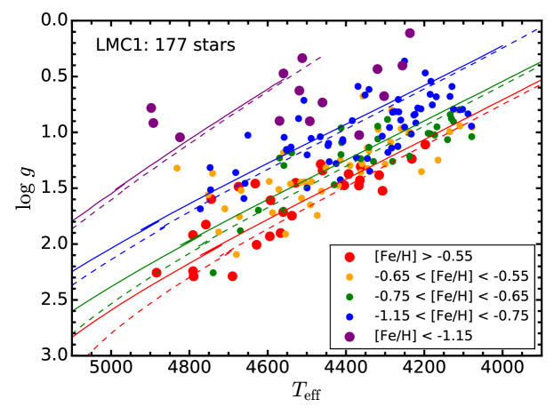
Finally, we compare the results of our reduced LMC1 sample to the predictions of stellar models from Bressan et al. (2012) in Figure 8. We applied a systematic offset of $-0.3$ dex to the log g scale of the stellar models to better match the data in a systematic sense. Given this shift, the overall trends and ranges of log g and $T_{\rm eff}$ expected in the models appears to fit the data reasonably well. Matching these isochrones represents a practical way to constrain the ages of individual RGs if their masses are well known. We discuss the limitations of such mass calculations in Section 5.1.

4.2. Metallicity Distribution Function

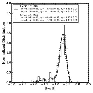
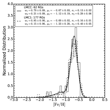
Figure 9 shows a set of MDFs derived from our reduced LMCC and LMC1 samples. In all cases, we have fit the observed MDFs (the histograms) with two Gaussian distributions (the curves; also known as the two Gaussian mixture model), each of which represents a population parameterized by a Gaussian mixture weight $w_{i}$, a mean value $\mu_{i}$ and a standard deviation $\sigma_{i}$. The Gaussian mixture weight is the fraction of a single Gaussian distribution relative to the sum of the two Gaussians, and all weights should sum to unity. The best-fit Gaussian parameters can be found in the legend of each panel in Figure 9.

C05 first fitted the MDF of the LMC bar by two populations. Their original MDF contains 373 RGs and can be best fitted by two Gaussian distributions as $(w_{1},\,\mu_{1},\,\sigma_{1})=(0.89,\,-0.37,\,0.15)$ and $(w_{2},\,\mu_{2},\,\sigma_{2})=(0.11,\,-1.08,\,0.46)$. One goal of our LMCC selection was to acquire a subsample from C05 without changing their original MDF. It can be confirmed—by the dashed histogram in Figure 9a with its best-fitting curve—that there is no significant difference between the MDF of the original C05 sample and the MDF of 131 stars. With this subsample of 131 stars, we also confirm that the fitting results of two Gaussian distributions are the best among one to ten Gaussian mixture models, and so is the case for all the following MDFs. Figure 9a also provides a direct comparison between the MDFs of the same 131 RGs from C05’s (dashed) and our (solid) metallicity measurements. Our MDF peaks at a lower metallicity for both the metal-rich and metal-poor populations; the differences relative to C05 are $\rm 0.27~{}dex\ and\ 0.14~{}dex$ (in the sense C05$-$M2FS), respectively.

In Figures 9b and 9c, we compare the MDFs between the LMCC and LMC1 samples. The LMC1 MDF remains the same in both figures, with the best-fit parameters as $(w_{1},\,\mu_{1},\,\sigma_{1})=(0.85\pm 0.06,\,-0.69\pm 0.02,\,0.16\pm 0.01)$ and $(w_{2},\,\mu_{2},\,\sigma_{2})=(0.15\pm 0.06,\,-1.23\pm 0.20,\,0.40\pm 0.05)$. The LMCC MDFs, on the other hand, are changed due to the different sample sizes: all 131 stars in the reduced LMCC sample are included in Figure 9b; while in Figure 9c, only the 62 stars are considered for being located in the same CMD region determined by the LMC1 sample (see Section 4.1 and Figure 6c). Both LMCC MDFs agree well with the LMC1 MDF.

One problem with all the MDFs mentioned above is that they may reflect biases due to the sample selection effects. Since the LMC1 sample was selected in a very specific manner (see Section 2.1 and Figure 3), it is feasible for us to correct the LMC1 MDF for its underlying selection bias. Our correction starts by counting stars within every rectangle shown in Figure 3. Within a given rectangle, the sub-MDF is corrected by multiplying a weight factor, which is a ratio of the total number of stars divided by the observed number of stars. This step is then carried out for all the rectangles, and all sub-MDFs are summed up before being renormalized to a final corrected MDF. The comparison between the corrected MDF and the ‘raw’ MDF from the reduced LMC1 sample is shown in Figure 9d. The corrected LMC1 MDF has a slightly higher mean for the metal-rich component but with the same fraction, and can now be fitted as $(w_{1},\,\mu_{1},\,\sigma_{1})=(0.85\pm 0.08,\,-0.66\pm 0.02,\,0.17\pm 0.01)$ and $(w_{2},\,\mu_{2},\,\sigma_{2})=(0.15\pm 0.08,\,-1.20\pm 0.24,\,0.41\pm 0.06)$. This correction can be applied in a reproducible manner to the LMC1 sample, but not to the LMCC sample due to the different and ill-defined selection method adopted by C05. As a result, the corrected MDF based on 177 stars in the LMC1 sample represents our best estimate of the MDF of the central LMC bar.

4.3. Kinematics

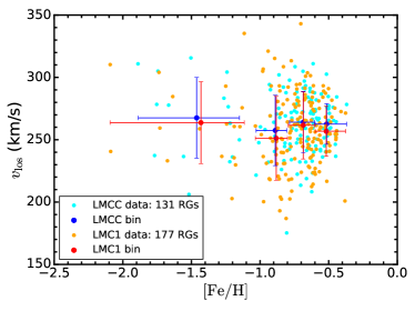
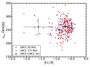
The heliocentric LOS velocities range between 175.2 km s^-1 and 343.1 km s^-1 for our full RG sample (including all the LMCC and LMC1 RGs), implying that all stars in our sample should be considered as LMC members according to Zhao et al. (2003). The mean heliocentric LOS velocity of 131 LMCC stars is $262.9\pm 2.1$ km s^-1 with a standard deviation of $24.4\pm 1.6$ km s^-1, compared to $258.1\pm 2.1$ km s^-1 and $28.3\pm 1.5$ km s^-1 for 177 LMC1 stars. For a combined sample of 239 RGs (i.e. all stars in Figures 6c and 6d), we measured a mean heliocentric LOS velocity of $258.5\pm 1.8$ km s^-1 with a velocity dispersion of $27.8\pm 1.3$ km s^-1, in good agreement with previous measurement of the LMC bar by C05.

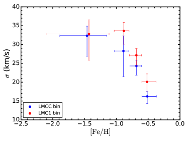
In Figure 10, we plot the heliocentric LOS velocities (left panels) and the corresponding velocity dispersions (right panels) both as a function of metallicity. The top panels show the kinematics of LMCC and LMC1 separately, while the bottom panels show the combined results from the two fields. In all cases, the whole sample is divided into four subsamples according to the metallicity bins in Table 6, in which we also report the mean heliocentric velocity and the corresponding velocity dispersion in each bin based on the sample of 239 RGs. It can be seen both in Figure 10 and Table 6 that the velocity dispersion increases significantly from $18.7\pm 1.9$ km s^-1 for the most metal-rich stars to $31.2\pm 4.3$ km s^-1 for the most metal-poor stars.

5. Summary and Discussion

In this paper, we have measured physical parameters for 312 stellar targets in the LMC bar from high-resolution spectra obtained with the multi-fiber facility M2FS on the Magellan/Clay Telescope. Assuming $E(V-I)=0.15\pm 0.07$ mag constantly, we initially estimated an effective temperature of each star from the OGLE-II $V-I$ color (Udalski et al., 2000) according to the color-temperature relation for giants (Ramírez & Meléndez, 2005). Then, each star’s LOS velocity, surface gravity and metallicity were fitted simultaneously by comparing each background-subtracted spectrum statistically with a library of template spectra made by synthetic modeling (Lee et al., 2008a, b).

All of our stellar spectra are obtained from two LMC bar fields, labelled as ‘LMCC’ and ‘LMC1’, respectively. Four of the 312 stellar targets are confirmed to be possible double-star sources. Among the remaining 308 stars, 177 LMC1 RGs are observed spectroscopically for the first time. The remaining 131 LMCC RGs were first observed by C05 and 39 were also subsequently observed by VdS13. The reobserved stars are used to directly compare the measurements of the physical parameters among studies. As a result, we found that our metallicity measurements gave a MDF with lower peaks of both metal-rich and metal-poor populations, comparing to C05. The differences in these populations are $\rm\Delta[Fe/H]=0.29\pm 0.02~{}dex\ and\ 0.12\pm 0.29~{}dex$, respectively, given the typical measurement errors in metallicity are 0.06 dex and 0.12 dex for us and C05.

Based on 177 RGs in the LMC1 sample, we measured a new mean metallicity in the LMC bar of $\rm[Fe/H]=-0.76\pm 0.02$ dex ($\sigma=0.28\pm 0.03$ dex) and generated a new sample-selection-effect corrected MDF for the LMC bar (Figure 9d). The MDF can be best fitted by two Gaussian distributions with a portion of $85\%$ and $15\%$, respectively. The majority population is made of the more metal-rich stars and has a mean value of $\rm[Fe/H]=-0.66\pm 0.02$ dex ($\sigma=0.17\pm 0.01$ dex), while the minority one is relatively metal-poor and has a mean $\rm[Fe/H]=-1.20\pm 0.24$ dex ($\sigma=0.41\pm 0.06$ dex). Our newly-observed MDF is different from that reported by C05 in two aspects: first, our metal-rich population peaks of about $0.29\pm 0.02$ dex lower than that found by C05; second, our metal-poor population fraction ($\approx 15$ %) is slightly larger than that ($\approx 11$ %) found by C05.

In both LMCC and LMC1 samples, the kinematics as a function of metallicity provides a good way to trace the evolution of the LMC bar (Figure 10). The kinematics also show a clear trend of the decreased velocity dispersion with increasing metallicity. This trend not only confirms that more metal-poor stellar populations are distinguished dynamically by metallicity, but also implies a true chemo-dynamical evolution of the bar that covers at least a few crossing times of the system. C05 found that there may exist an old, thicker disk or halo population in the LMC bar with a velocity dispersion $40.8\pm 1.7$ km s^-1 among the most metal-poor stars in their sample ($5\ \%$). Our results indicate the existence of the thicker component in the LMC bar, though a smaller value $31.2\pm 4.3$ km s^-1 is measured from our most metal-poor ($\approx 10$ %) stars. This reflects the kinematics of the old populations in the LMC bar, and is in good agreement with the velocity dispersion of 30 km s^-1 for RR Lyrae stars (Gratton et al., 2004).

5.1. Stellar Masses: A Cautionary Tale

The ultimate aim of this study is to map the chemo-dynamical properties as a function of position and age, such as the age-metallicity relation and the star formation history of the LMC bar. To take the first step, we compared our spectroscopic results with PARSEC isochrones (Bressan et al., 2012) in Figure 8, which provides a way to measure the age of a RG if its mass is well constrained.

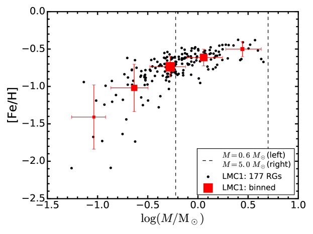
To calculate the masses of the LMC1 RGs, we followed the method introduced by Feuillet et al. (2016) who used the well-known relations $L=4\pi R^{2}\sigma T^{4}_{\rm eff}$ and $g=GM/R^{2}$ (where $\sigma$ is the Stefan-Boltzmann constant and $G$ is the gravitational constant). In our calculation, the luminosities were calculated from apparent OGLE-II $V$-band magnitudes, the distance modulus to the LMC ($18.50\pm 0.06$ mag, Pietrzyński et al., 2009), a constant extinction ($A_{V}=0.34$ mag), and the bolometric corrections (BCs) interpolated from the model-based BC tables the dustyAGB07 database, Marigo et al., 2008; Girardi et al., 2008. We also used the solar bolometric magnitude $M_{\rm Bol,\,\odot}=4.77$ mag and luminosity $L_{\odot}=3.844\times 10^{33}$ erg/s (Bahcall et al., 1995). Shown in Figure 11 are the calculated masses as a function of metallicity. To elucidate the relation between mass and metallicity, we binned our sample by mass and calculated a mean metallicity for each bin (red squares). It can be seen that the mean metallicity increases with mass increasing, or equivalently with age decreasing. This phenomenon is similar to the one found by C05 on their age-metallicity relation.

But an important problem with our mass calculation is evident in Figure 11: The expected mass of RGs in this portion of the CMD would be expected to be in a range spanning approximately from 0.6 to 5 $\rm M_{\odot}$ (see the two dashed vertical lines in Figure 11). However, a significant number of our RGs have calculated masses below the lower limit. Due to this anomalously large range of masses from our simple calculation, it seems impossible to derive reliable ages from any RG mass-age relation (e.g. from the PARSEC isochrones). The origin of the discrepancy in our mass/age scale remains unclear and would not be solved by a simple offset in $\log{g}$ or in our $T_{\rm eff}$ scale. We note that C05 and Feuillet et al. (2016) encountered similar problems, though to a different quantitative extent. Therefore, we limit ourselves in concluding that there is an age-metallicity relation within the bar with a positive slope over most of the age sampled by normal RGs. Although the potential for extracting the age-metallicity distribution from multiplexed spectroscopy of field stars in the LMC bar is evident from this discussion, improved stellar parameters—particularly log g values—will be needed to fully exploit this approach.

Table 1Summary of the observations in the LMC bar

Field	$\alpha_{2000}$	$\delta_{2000}$	UT Date	Num. of Exp.	Total Exp. Time
Designation	(h:m:s)	(∘:$\arcmin$:$\arcsec$)			(s)
LMC1	05:22:11.09	-69:45:52.3	Dec 23, 2014	3	3900
LMC1 (Background)			Nov 18, 2015	3	1800
LMCC	05:24:35.96	-69:50:09.4	Nov 15, 2015	3	5400

Table 2Sample selected in the LMC bar

ID	$\alpha_{2000}$	$\delta_{2000}$	V	I	Notea
	(h:m:s)	(∘:$\arcmin$:$\arcsec$)	(mag)	(mag)
LMCC-b001	05:25:26.76	-70:02:31.9	$17.320\pm 0.024$	$15.893\pm 0.024$	05252676-7002318
LMCC-b002	05:25:25.99	-70:01:43.0	$17.353\pm 0.015$	$15.786\pm 0.015$	05252599-7001429
LMCC-b003	05:25:23.63	-70:01:05.1	$17.406\pm 0.013$	$16.012\pm 0.013$	05252362-7001051
LMCC-b004	05:25:31.26	-70:01:02.9	$17.418\pm 0.013$	$16.057\pm 0.013$	05253125-7001028
LMCC-b005	05:25:29.58	-69:59:23.4	$17.588\pm 0.018$	$16.496\pm 0.018$	05252958-6959234
$\cdots$
LMC1-b002	05:23:17.12	-69:55:29.9	$17.654\pm 0.064$	$16.128\pm 0.064$	5-138140
LMC1-b003	05:23:14.46	-69:53:45.1	$17.983\pm 0.049$	$16.554\pm 0.049$	5-145482
LMC1-b004	05:23:37.49	-69:52:42.3	$17.590\pm 0.035$	$16.220\pm 0.035$	5-145352
LMC1-b005	05:23:21.80	-69:51:35.1	$17.967\pm 0.053$	$16.834\pm 0.053$	5-153086
LMC1-b006	05:23:32.77	-69:50:51.2	$18.036\pm 0.069$	$16.732\pm 0.069$	5-153131
$\cdots$

^a Note: 2MASS ID for LMCC targets; OGLE-II ID for LMC1 targets

Table 3Fits to twilight spectra for SSPP^a library

Field	$\langle\overline{v_{\rm los}}-v_{\rm los,\odot}\rangle$	$\sigma_{\overline{v_{\rm los}}}$	$\langle\overline{\log{g}}-\log{g_{\odot}\rangle}$	$\sigma_{\overline{\log{g}}}$	$\langle\overline{\rm[Fe/H]}-{\rm[Fe/H]}_{\odot}\rangle$	$\sigma_{\overline{\rm[Fe/H]}}$
	(km s-1)	(km s-1)	(dex)	(dex)	(dex)	(dex)
LMCC-b	$-2.36$	0.18	$0.01$	0.04	$-0.18$	0.02
LMCC-r	$-2.69$	0.17	$0.02$	0.04	$-0.18$	0.02
LMC1-b	$-0.53$	0.22	$-0.01$	0.04	$-0.20$	0.02
LMC1-r	$-0.35$	0.22	$0.00$	0.04	$-0.19$	0.02

^a library of Lee et al. (2008a, b)

Table 4Stellar parameters of the sample in the LMC bar

ID	$S/N$	$v_{\rm los}$	$T_{\rm eff}$	$\log{[g/(\rm cm\ s^{-2})]}$	[Fe/H]
		(km s-1)	(K)	(dex)	(dex)
LMCC-b001	11.8	$271.2\pm 0.3$	$4250\pm 100$	$1.20\pm 0.09$	$-0.63\pm 0.05$
LMCC-b002	13.3	$259.3\pm 0.3$	$4085\pm 75$	$1.00\pm 0.07$	$-0.54\pm 0.05$
LMCC-b003	15.1	$283.7\pm 0.3$	$4295\pm 99$	$1.15\pm 0.07$	$-0.73\pm 0.04$
LMCC-b004	13.3	$223.3\pm 0.3$	$4341\pm 106$	$1.33\pm 0.08$	$-0.62\pm 0.05$
LMCC-b005	13.8	$315.7\pm 0.4$	$4822\pm 161$	$1.11\pm 0.18$	$-1.50\pm 0.05$
$\cdots$
LMC1-b002	10.3	$303.7\pm 0.3$	$4134\pm 106$	$0.84\pm 0.08$	$-0.65\pm 0.05$
LMC1-b003	9.6	$278.4\pm 0.4$	$4250\pm 112$	$0.95\pm 0.09$	$-0.75\pm 0.05$
LMC1-b004	11.1	$243.7\pm 0.4$	$4330\pm 114$	$1.26\pm 0.09$	$-0.65\pm 0.05$
LMC1-b005	9.9	$268.2\pm 0.4$	$4758\pm 199$	$1.83\pm 0.14$	$-0.48\pm 0.05$
LMC1-b006	12.3	$277.7\pm 0.4$	$4430\pm 161$	$1.47\pm 0.09$	$-0.72\pm 0.05$
$\cdots$

Table 5Metallicity comparisons for 11 stars from the LMCC sample

ID	$S/N$	$T_{\rm eff}$	$\log{g}$	[Fe/H]BA	[Fe/H]EW	[FeI/H]V13	[Fe/H]C05
		(K)	(dex)	(dex)	(dex)	(dex)	(dex)
LMCC-b027	11.5	$4886\pm 174$	$2.10\pm 0.16$	$-0.69\pm 0.06$	$-1.34\pm 0.40$	$-0.38\pm 0.13$	$-0.43\pm 0.14$
LMCC-b075	13.6	$4278\pm 140$	$0.90\pm 0.08$	$-0.82\pm 0.05$	$-0.26\pm 0.20$	$-0.56\pm 0.13$	$-0.53\pm 0.13$
LMCC-b084	12.1	$5107\pm 201$	$1.25\pm 0.18$	$-0.49\pm 0.05$	$-0.30\pm 0.50$	$-0.24\pm 0.11$	$-0.48\pm 0.14$
LMCC-b085	10.4	$4922\pm 177$	$3.22\pm 0.12$	$-0.44\pm 0.07$	$-0.74\pm 0.33$	$-0.83\pm 0.10$	$-0.50\pm 0.13$
LMCC-b094	15.9	$4951\pm 168$	$1.25\pm 0.18$	$-1.77\pm 0.05$	$-2.06\pm 0.37$	$-1.42\pm 0.16$	$-1.55\pm 0.10$
LMCC-b106	10.4	$4237\pm 123$	$0.75\pm 0.09$	$-0.77\pm 0.05$	$-1.38\pm 0.34$	$-0.40\pm 0.17$	$-0.44\pm 0.14$
LMCC-b110	11.0	$4154\pm 81$	$1.07\pm 0.08$	$-0.59\pm 0.05$	$-0.94\pm 0.24$	$-0.23\pm 0.22$	$-0.16\pm 0.14$
LMCC-r043	17.6	$4298\pm 100$	$1.46\pm 0.08$	$-0.47\pm 0.05$	$-0.62\pm 0.21$	$-0.69\pm 0.12$	$-0.20\pm 0.14$
LMCC-r064	19.9	$4397\pm 106$	$1.01\pm 0.08$	$-0.93\pm 0.04$	$-0.88\pm 0.29$	$-0.58\pm 0.11$	$-1.42\pm 0.13$
LMCC-r068	18.3	$4870\pm 169$	$0.84\pm 0.13$	$-0.50\pm 0.04$	$-0.46\pm 0.41$	$-0.25\pm 0.12$	$-0.33\pm 0.14$
LMCC-r078	17.2	$4952\pm 180$	$0.73\pm 0.12$	$-0.45\pm 0.04$	$-0.36\pm 0.45$	$-0.12\pm 0.11$	$-0.30\pm 0.14$

Table 6Kinematics versus metallicity for 239 stars

[Fe/H] bin	$N_{\rm star}$	$\overline{v_{\rm los}}$	$\sigma_{v}$
		(km s-1)	(km s-1)
$[-2.09,-1.10]$	23	$261.8\pm 6.7$	$31.2\pm 4.3$
$[-1.10,-0.80]$	58	$251.1\pm 4.3$	$32.7\pm 2.8$
$[-0.80,-0.60]$	99	$262.3\pm 2.8$	$27.4\pm 1.8$
$[-0.60,-0.38]$	59	$258.2\pm 2.5$	$18.7\pm 1.9$

Figure 1.— Schematic map of the LMC bar, showing the locations of our observed fields (solid circles) relative to the bar and other prominent features in the LMC. The dashed rectangle shows the region containing seven FORS2 pointings from C05 (see their Figure 2). The spectroscopic targets reported in this work are located in the LMC1 (red circle) and LMCC (black circle) fields. The red filled square shows the densest point in the LMC bar as defined by van der Marel (2001), and the red filled triangle represents the stellar dynamical center inferred from a model fit to the third-epoch HST proper motions by van der Marel & Kallivayalil (2014).

Figure 2.— The color-magnitude diagram of the LMC bar with our selected RG targets highlighted for each field shown in Figure 1. The smaller black dots represent the $V$ and $I$ band photometry from OGLE-II catalogue (Udalski et al., 2000) of all stellar candidates in the LMC1 field defined Figure 1. The larger dots represent the targets we selected for spectroscopic observation: black for the LMCC sample and red for the LMC1 sample (see Figure 1). Note that the LMCC targets were selected from the transformed CTIO photometry according to C05, while the LMC1 ones were selected from OGLE-II photometry directly. The two red dashed lines show the upper and left boundaries for our LMC1 selection criteria on the CMD. Black curves are the isochrones from Bressan et al. (2012) for an age of 6 Gyr and $\rm[Fe/H]=-2.2$ (left), $-0.6$ (middle) and 0.0 (right) dex, respectively. The isochrones are plotted assuming $E(V-I)=0.15$ mag and $A_{I}=0.20$ mag.

Figure 3.— The RG selection criteria in the LMC1 field. The small black dots represent the OGLE-II photometry of all stars in this field. Six candidates were selected within each red rectangle.

Figure 4.— A sample of selected background-subtracted M2FS spectra (black) in the LMCC (left panels) and LMC1 (right panels) fields, with best-fitting models (red). Text lists target ID, median SNR per pixel, and our measurements of $v_{\rm los}$, $T_{\rm eff}$, $\log g$, and ${\rm[Fe/H]}$. In both fields, we selected the sample spectra of high-SNR metal-rich (top panel), high-SNR metal-poor (second panel), low-SNR metal-rich (third panel) and low-SNR metal-poor (bottom panel), respectively.

Figure 5.— Comparison of the physical parameters measured in this study to those measured by C05 (top panels) and VdS13 (middle and bottom panels). Dashed lines indicate 1:1 relation. Note that the error bars of $v_{\rm los,\,M2FS}$ and $v_{\rm los,\,VdS13}$ in (a) and (c) are smaller than size of the dots.

Figure 6.— The spectroscopic HR diagram on the $T_{\rm eff}$-$\log{g}$ plane color-coded by metallicity bins (see the legend). Note that we only plot the error bars of the stars in the most metal-rich (red) and the most metal-poor (purple) bins.

Figure 7.— The spectra (black) and their best-fit models (red) for the two anomalous stellar targets in the LMC1 sample. Left panels: results of a single-star model; right panels: results of a double-star model with the first component in blue and the second one in green. The best-fit parameters are also shown in each panel.

Figure 8.— The HR diagram similar to Figure 6d but with comparison to PARSEC isochrones (Bressan et al., 2012) of 5 Gyr (solid curves) and 12.7 Gyr (dashed curves), respectively. The color dots are coded by metallicity as shown in the legend. The isochrones are color-coded by $\rm[Fe/H]=-0.5$ (red), $-0.7$ (green), $-1.1$ (blue) and $-2.2$ (purple), respectively. We applied a systematic offset of 0.3 dex in log g of the isochrones.

Figure 9.— The MDFs from different RG samples with the best fits by a mixture of two Gaussian distributions. The legends list the normalized weight $w_{i}$, mean $\mu_{i}$ and standard deviation $\sigma_{i}$ for each Gaussian component. (a) Top-left panel shows the MDFs of the same 131 RGs with metallicities measured with M2FS (solid) versus that measured by C05 (dashed). (b) Top-right panel shows the MDFs of 131 RGs from LMCC (solid) and of 177 RGs from LMC1 (dashed), using the metallicities measured with M2FS only. (c) Bottom-left panel shows the MDF of 62 RGs from LMCC (solid) that locate in the same LMC1 sample region on CMD, using the metallicities measured with M2FS only; the dashed MDF is the same as that in the top-right panel. (d) Bottom-right panel: the MDF of 177 LMC1 RGs with selection effect correction (solid), comparing to the ‘raw’ MDF (dashed).

Figure 10.— The heliocentric LOS velocities (left panels) and velocity dispersions (right panels) from M2FS spectra as a function of metallicity. The samples are binned by metallicity as shown in Table 6. The top panels show the LMCC and LMC1 samples separately, and the bottom panels show their combined sample. The horizontal error bars indicate the full range values in each bin, and the vertical error bars are the standard deviations of the velocities (left panels) and velocity dispersions (right panels) in each bin, respectively.

Figure 11.— The masses of the LMC1 RGs as a function of metallicity. The black dots represent the individual stars. The red squares represent the binned results (mean values in $\rm[Fe/H]$ and $\log{M}$), with their sizes indicating the sample sizes; the horizontal error bars are made to cover the full mass ranges in each bin, while the vertical error bars show the standard deviations of metallicity.

References

- Bahcall et al. (1995) Bahcall, J. N., Pinsonneault, M. H., & Wasserburg, G. J. 1995, Reviews of Modern Physics, 67, 781
- Bekki (2009) Bekki, K. 2009, MNRAS, 393, L60
- Besla et al. (2012) Besla, G., Kallivayalil, N., Hernquist, L., et al. 2012, MNRAS, 421, 2109
- Bica et al. (1999) Bica, E. L. D., Schmitt, H. R., Dutra, C. M., & Oliveira, H. L. 1999, AJ, 117, 238
- Bothun & Thompson (1988) Bothun, G. D., & Thompson, I. B. 1988, AJ, 96, 877
- Bressan et al. (2012) Bressan, A., Marigo, P., Girardi, L., et al. 2012, MNRAS, 427, 127
- Carrera et al. (2011) Carrera, R., Gallart, C., Aparicio, A., & Hardy, E. 2011, AJ, 142, 61
- Carrera et al. (2008) Carrera, R., Gallart, C., Hardy, E., Aparicio, A., & Zinn, R. 2008, AJ, 135, 836
- Cole et al. (2005) Cole, A. A., Tolstoy, E., Gallagher, III, J. S., & Smecker-Hane, T. A. 2005, AJ, 129, 1465
- de Vaucouleurs et al. (1991) de Vaucouleurs, G., de Vaucouleurs, A., Corwin, Jr., H. G., et al. 1991, S&T, 82, 621
- de Vaucouleurs & Freeman (1972) de Vaucouleurs, G., & Freeman, K. C. 1972, Vistas in Astronomy, 14, 163
- Eggen (1971) Eggen, O. J. 1971, ApJ, 165, 317
- Feroz & Hobson (2008) Feroz, F., & Hobson, M. P. 2008, MNRAS, 384, 449
- Feroz et al. (2009) Feroz, F., Hobson, M. P., & Bridges, M. 2009, MNRAS, 398, 1601
- Feroz et al. (2013) Feroz, F., Hobson, M. P., Cameron, E., & Pettitt, A. N. 2013, ArXiv e-prints, arXiv:1306.2144
- Feuillet et al. (2016) Feuillet, D. K., Bovy, J., Holtzman, J., et al. 2016, ApJ, 817, 40
- Geisler et al. (1997) Geisler, D., Bica, E., Dottori, H., et al. 1997, AJ, 114, 1920
- Girardi et al. (2000) Girardi, L., Bressan, A., Bertelli, G., & Chiosi, C. 2000, A&AS, 141, 371
- Girardi et al. (2008) Girardi, L., Dalcanton, J., Williams, B., et al. 2008, PASP, 120, 583
- Gratton et al. (2004) Gratton, R. G., Bragaglia, A., Clementini, G., et al. 2004, A&A, 421, 937
- Hinkle et al. (2000) Hinkle, K., Wallace, L., Valenti, J., & Harmer, D. 2000, Visible and Near Infrared Atlas of the Arcturus Spectrum 3727-9300 A
- Holtzman et al. (1999) Holtzman, J. A., Gallagher, III, J. S., Cole, A. A., et al. 1999, AJ, 118, 2262
- Kallivayalil et al. (2006) Kallivayalil, N., van der Marel, R. P., Alcock, C., et al. 2006, ApJ, 638, 772
- Kallivayalil et al. (2013) Kallivayalil, N., van der Marel, R. P., Besla, G., Anderson, J., & Alcock, C. 2013, ApJ, 764, 161
- Kim et al. (1998) Kim, S., Staveley-Smith, L., Dopita, M. A., et al. 1998, ApJ, 503, 674
- Kormendy & Kennicutt (2004) Kormendy, J., & Kennicutt, Jr., R. C. 2004, ARA&A, 42, 603
- Kramida et al. (2015) Kramida, A., Ralchenko, Y., Reader, J., & NIST ASD Team. 2015, NIST Atomic Spectra Database (version 5.3), [Online]
- Lapenna et al. (2012) Lapenna, E., Mucciarelli, A., Origlia, L., & Ferraro, F. R. 2012, ApJ, 761, 33
- Lee et al. (2008a) Lee, Y. S., Beers, T. C., Sivarani, T., et al. 2008a, AJ, 136, 2022
- Lee et al. (2008b) —. 2008b, AJ, 136, 2050
- Liu et al. (2011) Liu, L., Gerke, B. F., Wechsler, R. H., Behroozi, P. S., & Busha, M. T. 2011, ApJ, 733, 62
- Marigo et al. (2008) Marigo, P., Girardi, L., Bressan, A., et al. 2008, A&A, 482, 883
- Mateo et al. (2012) Mateo, M., Bailey, J. I., Crane, J., et al. 2012, in Proc. SPIE, Vol. 8446, Ground-based and Airborne Instrumentation for Astronomy IV, 84464Y
- Mermilliod (1981) Mermilliod, J. C. 1981, A&A, 97, 235
- Meynet et al. (1993) Meynet, G., Mermilliod, J.-C., & Maeder, A. 1993, A&AS, 98, 477
- Olsen et al. (2011) Olsen, K. A. G., Zaritsky, D., Blum, R. D., Boyer, M. L., & Gordon, K. D. 2011, ApJ, 737, 29
- Olszewski et al. (1996) Olszewski, E. W., Suntzeff, N. B., & Mateo, M. 1996, ARA&A, 34, 511
- Pardy et al. (2016) Pardy, S. A., D’Onghia, E., Athanassoula, E., Wilcots, E. M., & Sheth, K. 2016, ArXiv e-prints, arXiv:1602.07689
- Piatek et al. (2008) Piatek, S., Pryor, C., & Olszewski, E. W. 2008, AJ, 135, 1024
- Pietrzyński et al. (2009) Pietrzyński, G., Thompson, I. B., Graczyk, D., et al. 2009, ApJ, 697, 862
- Pompéia et al. (2008) Pompéia, L., Hill, V., Spite, M., et al. 2008, A&A, 480, 379
- Ramírez & Allende Prieto (2011) Ramírez, I., & Allende Prieto, C. 2011, ApJ, 743, 135
- Ramírez & Meléndez (2005) Ramírez, I., & Meléndez, J. 2005, ApJ, 626, 465
- Robotham et al. (2012) Robotham, A. S. G., Baldry, I. K., Bland-Hawthorn, J., et al. 2012, MNRAS, 424, 1448
- Roederer et al. (2014) Roederer, I. U., Preston, G. W., Thompson, I. B., et al. 2014, AJ, 147, 136
- Smecker-Hane et al. (2002) Smecker-Hane, T. A., Cole, A. A., Gallagher, III, J. S., & Stetson, P. B. 2002, ApJ, 566, 239
- Sneden (1973) Sneden, C. A. 1973, PhD thesis, THE UNIVERSITY OF TEXAS AT AUSTIN.
- Sobeck et al. (2011) Sobeck, J. S., Kraft, R. P., Sneden, C., et al. 2011, AJ, 141, 175
- Staveley-Smith et al. (2003) Staveley-Smith, L., Kim, S., Calabretta, M. R., Haynes, R. F., & Kesteven, M. J. 2003, MNRAS, 339, 87
- Szymanski (2005) Szymanski, M. K. 2005, Acta Astron., 55, 43
- Tollerud et al. (2011) Tollerud, E. J., Boylan-Kolchin, M., Barton, E. J., Bullock, J. S., & Trinh, C. Q. 2011, ApJ, 738, 102
- Udalski et al. (1997) Udalski, A., Kubiak, M., & Szymanski, M. 1997, Acta Astron., 47, 319
- Udalski et al. (2000) Udalski, A., Szymanski, M., Kubiak, M., et al. 2000, Acta Astron., 50, 307
- van der Marel (2001) van der Marel, R. P. 2001, AJ, 122, 1827
- van der Marel et al. (2002) van der Marel, R. P., Alves, D. R., Hardy, E., & Suntzeff, N. B. 2002, AJ, 124, 2639
- van der Marel & Kallivayalil (2014) van der Marel, R. P., & Kallivayalil, N. 2014, ApJ, 781, 121
- Van der Swaelmen et al. (2013) Van der Swaelmen, M., Hill, V., Primas, F., & Cole, A. A. 2013, A&A, 560, A44
- van Dokkum (2001) van Dokkum, P. G. 2001, PASP, 113, 1420
- Walker et al. (2015a) Walker, M. G., Mateo, M., Olszewski, E. W., et al. 2015a, ApJ, 808, 108
- Walker et al. (2015b) Walker, M. G., Olszewski, E. W., & Mateo, M. 2015b, MNRAS, 448, 2717
- Wilcots & Prescott (2004) Wilcots, E. M., & Prescott, M. K. M. 2004, AJ, 127, 1900
- Yozin & Bekki (2014) Yozin, C., & Bekki, K. 2014, MNRAS, 439, 1948
- Zhao et al. (2003) Zhao, H., Ibata, R. A., Lewis, G. F., & Irwin, M. J. 2003, MNRAS, 339, 701