Entanglement harvesting and divergences in quadratic Unruh-DeWitt detectors pairs
Abstract
We analyze correlations between pairs of particle detectors quadratically coupled to a real scalar field. We find that, while a single quadratically coupled detector presents no divergences, when one considers pairs of detectors there emerge unanticipated persistent divergences (not regularizable via smooth switching or smearing) in the entanglement they acquire from the field. We have characterized such divergences, discussed whether a suitable regularization can allow for fair comparison of the entanglement harvesting ability of the quadratic and the linear couplings, and finally we have found a UV-safe quantifier of harvested correlations. Our results are relevant to future studies of the entanglement structure of the fermionic vacuum.
pacs:
Valid PACS appear hereI Introduction
The vacuum state of a quantum field displays quantum correlations between observables defined in spacelike separated regions Summers and Werner (1985, 1987). This vacuum entanglement has been studied in quantum foundations, and has found a variety of applications such as quantum energy teleportation Hotta (2009, 2010), the black hole information loss problem Susskind et al. (1993) and firewalls, along with black hole complementarity Almheiri et al. (2013); Braunstein et al. (2013).
In a phenomenon called entanglement harvesting Salton et al. (2015), correlations in a quantum field (such as the electromagnetic field) can be swapped to particle detectors (such as atoms or qubits). This is possible even when the particle detectors remain spacelike separated throughout the duration of their interaction with the field. This was first shown by Valentini Valentini (1991) and later by Reznik et al. Reznik (2003); Benni Reznik (2005).
Since then, entanglement harvesting has been shown to be sensitive to the background geometry of spacetime Steeg and Menicucci (2009); Martín-Martínez and Menicucci (2012, 2014), as well as the topology Martín-Martínez et al. (2016). Additionally, it has been shown that entanglement harvesting can be done sustainably and distilled into Bell pairs in a process called entanglement farming Martín-Martínez et al. (2013), a protocol that can be adapted to create a quantum seismometer Brown et al. (2014). Entanglement harvesting has also been studied in detail in timelike separation contexts Olson and Ralph (2012, 2011) with implementation proposals in different testbeds from quantum key distribution based on homodyne detection Ralph and Walk (2015) to strongly coupled superconducting qubits Sabín et al. (2012).
To model the entanglement-swapping interaction between the detectors and field, the Unruh-DeWitt detector model is used. This model utilizes a first-quantized system (called a detector) linearly coupled to a scalar bosonic field. While most of our knowledge of entanglement harvesting has been gleaned from this setup Steeg and Menicucci (2009); Martín-Martínez and Menicucci (2012); Martín-Martínez et al. (2013); Martín-Martínez and Menicucci (2014); Brown et al. (2014); Martín-Martínez et al. (2016); Pozas-Kerstjens et al. (2017), there has been some exploration of more realistic models such as electromagnetic coupling of atoms Pozas-Kerstjens and Martín-Martínez (2016). All these studies, however, analyzed entanglement harvesting form bosonic fields.
It is known from fundamental studies that there are differences between the entanglement structure of the vacuum of fermionic and bosonic fields Alsing et al. (2006); Martín-Martínez and León (2009, 2010a, 2010b); Fuentes et al. (2010); Bruschi et al. (2010); Martín-Martínez et al. (2010); Martín-Martínez and Fuentes (2011); Montero and Martín-Martínez (2011a, b, 2011); Montero et al. (2011); Friis et al. (2011); Brádler and Jáuregui (2012); Montero and Martín-Martínez (2012a); Friis et al. (2012); Montero and Martín-Martínez (2012b); Friis et al. (2013). However, a study of entanglement harvesting in fermionic setups has never been performed. A study of detector-based entanglement harvesting from a fermionic vacuum could resolve ambiguities in defining entanglement measures between disjoint regions of a fermionic field Montero and Martín-Martínez (2011a, a); Montero et al. (2011); Friis et al. (2011); Brádler and Jáuregui (2012); Montero and Martín-Martínez (2012a); Friis et al. (2012); Montero and Martín-Martínez (2012b); Friis et al. (2013). The reasons why this has not been done can be traced back to fundamental difficulties associated with particle detector models for fermionic fields.
To analyze fermionic fields form the perspective of localized particle detectors a detector model was introduced that consisted of a cavity coupled to a fermionic field Iyer and Kumar (1980), much like Unruh’s original detector was a cavity coupled to a bosonic field Unruh (1976). Later, Takagi introduced an UDW-like model for fermionic fields Takagi (1985, 1986), wherein a two level system coupled quadratically to a fermionic field,
| (1) |
However, this model contained persistent divergences that could not be regularized by an appropriate choice of switching and smearing functions, as it was found in Hümmer et al. (2016). Thus, these investigations restricted themselves to studying transition rates instead of transition probabilities. To track down the origin of these divergences in Takagi’s fermionic detector, Hümer et al. studied three types of quadratically coupled UDW-like detectors Hümmer et al. (2016). They concluded that these divergences are mainly due to the detector coupling quadratically to the field instead of resulting from the analytic structure (spinor vs. scalar) or statistics (fermionic vs. bosonic) of the fields involved. Persistent divergences in the single-detector vacuum excitation probabilities (VEP) of quadratic UDW detectors were found to be renormalizable by the same techniques used in QED Hümmer et al. (2016), i.e. normal ordering the interaction Hamiltonian.
The analysis in Hümmer et al. (2016), however, was limited to a single detector coupled to the field. It is therefore natural to extend the studies of the quadratic coupling to fermions to settings of many detectors to explore, for example, entanglement harvesting from a fermionic vacuum. Nevertheless, before moving to the fermionic coupling, it is important to understand how entanglement harvesting works for detectors quadratically coupled to a bosonic field, so as to determine how much of any new phenomenology would be due to the fermionic nature of the field and how much of it is due to the quadratic nature of the coupling.
In this paper we extend the notion of entanglement harvesting to a detector coupled quadratically to a bosonic field. While this does not answer open questions about entanglement ambiguities in fermionic fields as posed in Montero and Martín-Martínez (2011a), it does shed light on differences between linearly and quadratically coupled detectors, which is one prominent difference between the bosonic and fermionic UDW models. A fermionic UDW model could resolve ambiguities in defining entanglement measures between disjoint regions of a fermionic field Montero and Martín-Martínez (2011a) and to this end it is important to understand how it is distinguished from its bosonic counterpart.
We find that, despite the finite renormalized single detector vacuum excitation probability, the two-detector density matrix remarkably contains persistent divergences at leading order in perturbation theory. These divergences cannot be regularized by means of a smooth switching function or spatial profile, nor are they renormalized by the techniques used in Hümmer et al. (2016). Instead, one must introduce additional means of regularization (e.g., a soft UV cutoff). It is interesting to note that these divergences appear only in the non-local contributions to the density matrix. As a result the entanglement harvested by detectors quadratically coupled to bosonic fields is sensitive to the choice of UV cutoff and may require further regularization.
To tackle the problem of entanglement harvesting with a pair of quadratically coupled detectors, we will follow two different avenues: a) We will analyze the nature and strength of the divergences in 3+1D flat spacetime, analyzing possible physically motivated regularization scales in entanglement harvesting and b) we will propose a measure of correlations between the detectors that are divergence free and use it to further our knowledge of the differences between the use of linear and quadratic couplings of particle detectors to study the entanglement structure of quantum fields.
This paper is organized as follows. In Section II we introduce the linear and quadratic UDW detector models and examine in detail their time evolution. In Section III we provide an overview of the single UDW detector, both quadratically and linearly coupled to a scalar bosonic field. Section IV analyzes the two-detector entanglement-harvesting set up; we show in detail how persistent divergences emerge in the non-local terms of the quadratically coupled two-detector system. In section V we compare the entanglement harvesting capabilities for the linear and quadratic models, first looking at entanglement harvesting under suitable UV-regularization and then studying a divergence free quantifier of harvested correlations from the field: the mutual information. We present our conclusions in section B.
II Time evolution of linear and quadratic detector models
Let us introduce the two different detector models that we will analyze and compare in this paper. First, let us consider the well-known UDW detector model. This model was first introduced as an operational way to study the particle content of a bosonic quantum field Unruh (1976); DeWitt (1979). It consists of a two-level quantum emitter (detector) coupled linearly to a scalar quantum field along its worldline.
For a single inertial detector (labelled A) in flat spacetime, the UDW interaction Hamiltonian in the interaction picture is given by
| (2) |
Here, the monopole moment represents the two-level internal degree of freedom of the detector, which couples linearly to a real massless scalar field . is the switching function that controls the time-dependence of the coupling of strength . The spatial profile carries information about the shape and size of the detector. The case of the point-like detector, commonly considered in the literature, is a particular case of (2) where the smearing function is a delta distribution, .
Modifications of this model where the detector is coupled quadratically to the field Hinton (1984) allow one to compare on equal footing the response of bosonic and fermionic detectors (the latter necessarily being quadratic Takagi (1986)). These models have been recently analyzed in detail in Hümmer et al. (2016). The interaction Hamiltonian for a quadratically coupled UDW detector is given by
| (3) |
where has been normal-ordered as prescribed by the analysis in Hümmer et al. (2016).
It is convenient at this point to define two different types of UV divergences that particle detector models may present. A regularizable divergence is one that can be removed by use of a smooth switching function and/or a smooth spatial profile (see, e.g., Louko and Satz (2008, 2006); Satz (2007)). A persistent divergence is one that remains even with smooth switching and smearing functions (such as the divergences renormalized in Hümmer et al. (2016)).
Analysis of the detector response function Louko and Satz (2008, 2006); Satz (2007) and a number of investigations of entanglement harvesting and quantum communication with (linear) UDW detectors Valentini (1991); Reznik (2003); Benni Reznik (2005); Pozas-Kerstjens and Martín-Martínez (2015); Jonsson et al. (2015); Blasco et al. (2015); Martín-Martínez and Louko (2015); Hotta (2009); Pozas-Kerstjens and Martín-Martínez (2016); Salton et al. (2015) indicate that all leading order UV divergences present in the time evolution of linearly coupled UDW detectors are regularizable. While this is not the case for quadratically coupled detectors Iyer and Kumar (1980); Hinton (1984); Takagi (1985, 1986), it has been shown that all persistent divergences can also be renormalized for an individual quadratically coupled detector Hümmer et al. (2016). We will demonstrate below that a straightforward application of the leading-order prescription in Hümmer et al. (2016) cannot renormalize persistent leading-order divergences in more complex scenarios with several detectors.
II.1 Time evolution of detector pairs
Previous studies of the quadratic UDW model focused on the response of a single detector Iyer and Kumar (1980); Hinton (1984); Takagi (1985, 1986); Hümmer et al. (2016). Since one of our goals is to analyze the model dependence of vacuum entanglement harvesting, we will also consider the evolution of two particle detectors coupled to the field vacuum.
Both the linear and quadratically coupled UDW Hamiltonians can be rewritten for the two-detector case as
| (4) | ||||
| (5) |
where is the label identifying detectors A and B. Note that the coupling strength in the quadratic case does not have the same dimensions as in the linear case.
If we let the initial state of the field-detector system be , its time evolved state is , where the label denotes the timescale where the switching function is non-zero, and the time evolution operator is given by the time-ordered exponential
| (6) |
Consequently, we can express the time evolution operator in terms of a Dyson expansion as
| (7) |
where
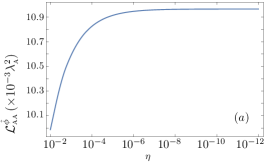
| (8) | ||||
| (9) |
We can express in a perturbative expansion as
| (10) |
where .
For our purposes we take as the initial state
| (11) |
with the field starting out in its lowest-energy (vacuum) state.
After time evolution, the time evolved partial state of the detectors is obtained by tracing out the field degrees of freedom:
| (12) |
The first order term does not contribute at all to the detectors’ dynamics for field states whose one-point function is zero. This includes Fock states, free thermal states and the vacuum state as a particular case of these two categories. In fact, for the vacuum state it can be easily proved that when is odd (see e.g., Pozas-Kerstjens and Martín-Martínez (2015)). Thus, we can express the time-evolved density matrix of the subsystem consisting of the two detectors as
| (13) |
where we have separated the local contributions to time evolution (proportional to and at leading order) from the non-local terms (responsible for the correlations the detectors acquire through the field) proportional to . Notice that, from (13), we can quickly recover the case of the evolution of a single detector just by taking .
Let us now particularize for the case where both detectors start out in the ground state:
| (14) |
It is convenient to pick the usual Pozas-Kerstjens and Martín-Martínez (2015) matrix representation for in the basis
| (15) |
In this basis, takes the form
| (16) |
where and depend on the nature of the coupling (e.g., linear versus quadratic, different switching and smearing functions, etc. See sections II.1.1 and II.1.2).
II.1.1 Linear coupling
The matrix elements of (16) for the linear coupling have been studied at length in the literature (See, for instance, Pozas-Kerstjens and Martín-Martínez (2015), which sets the notation that we will follow here) and are given by
| (17) | ||||
| (18) | ||||
where, assuming and are real, and are given by
| (19) | ||||
| (20) |
and the Wightman function, , is given by
| (21) |
To find an explicit expression for the Wightman function, we will utilize a plane-wave mode expansion of the field operator with soft UV cutoff ,
| (22) |
Here, (and ) are creation (and annihilation) operators which satisfy the canonical commutation relations .
Typically, the introduction of could be associated with a regularization procedure that leads to the usual pole prescription, in which the limit is well-defined and eventually taken when evaluating observable quantities. However can also be viewed as an ad hoc screening of the detector’s sensitivity to high frequency modes of the field (soft UV cutoff). This would effectively model, for example, a frequency dependent coupling strength where a detector does not couple to frequencies much larger than . When giving this kind of interpretation to the -regularization one should be careful with possible non-localities introduced in the theory due to a finite value of Martín-Martínez (2015). Although this point will not be relevant when the limit is well defined, it must be taken into account when managing possibly UV divergent terms, especially in the case of the quadratic coupling (3), as we will see below.
The Wightman function (21) for the linear coupling case can be written as
| (23) |
as it is easy to check, for example, through the usual plane-wave expansion in Eq. (22). Particularizing to 3+1 dimensions, the two-point function becomes
| (24) |
Note here that we see takes the form of the usual pole prescription for the Wightman function.
II.1.2 Quadratic coupling
For the quadratic coupling case in (5), the elements of the density matrix (16) take the following form
| (25) | ||||
| (26) |
which is structurally the same as in the linear coupling case. Indeed, and are also defined as in Eqs. (20) and (19), respectively. Thus, the difference between the usual UDW detector and the quadratically coupled UDW detector comes at the level of the functional . For the quadratically coupled model, is the vacuum expectation of the normal ordering of the square of the field operator at two different points, as given by
| (27) |
In Appendix A we show that the correlation functions and satisfy the following relation
| (28) |
which allows us to write explicitly as
| (29) | ||||
If we particularize to 3+1 dimensions, the correlation function is
| (30) |
Note here that the correlator for the quadratic UDW detector has a higher power polynomial in and in its denominator than does the usual correlator for the linear UDW detector.
III Single detector vacuum excitation probability in 3+1 dimensions,
| Dimensionless | ||
|---|---|---|
| variable | Expression | Physical meaning |
| Energy gap | ||
| UV cutoff | ||
| Detectors’ separation | ||
| switch-on times | ||
| Detectors’ size | ||
| — |
In this section we will briefly review the vacuum excitation probability (VEP) of a single detector for the usual linear UDW detector model and the more recently studied VEP for a quadratically coupled model Hümmer et al. (2016). The vacuum excitation probability is the probability of excitation of a single UDW detector initialized in its ground state in the vacuum.
It is well known that in 3+1 dimensions, point-like linearly coupled UDW detectors with sharp switching functions suffer regularizable UV divergences, which we recall can be eliminated by introducing a smooth switching or smearing function Louko and Satz (2006); Satz (2007); Louko and Satz (2008). However, quadratic UDW models (such as the quadratic scalar model introduced by Hinton in Hinton (1984), the cavity detector coupled to a fermionic field Iyer and Kumar (1980), or the fermionic UDW-like detector model introduced in Takagi (1985, 1986)) have VEPs that present persistent divergences (not removable with a smooth switching and/or smearing). These persistent divergences can, however, be renormalized with techniques analogous to those in QED Hümmer et al. (2016). Once renormalized, the quadratically coupled single-detector UDW model is regularizable both in its scalar and fermionic variants.
To find the time evolved state of a single (quadratically or linearly coupled) detector, we begin with the density matrix (16), then set . It is then simple to trace out detector B to find the single-detector reduced state,
| (31) |
in the basis , . The element of (31), , given in Eq. (18), is the vacuum excitation probability of detector A.
The vacuum excitation probability expressed as Eq. (18) is quite general and can be particularized to any spacetime dimensionality, switching function and spatial profile. For this analysis we will use smooth switching and spatial smearing functions which are only strongly supported in a finite region ( and respectively). Smooth switching and smearing will ensure the removal of all regularizable divergences of the kind studied in Louko and Satz (2008). In particular, we choose Gaussian switching and Gaussian smearing,
| (32) |
| (33) |
As mentioned previously, in the literature UDW detectors are often considered to be point-like. Notice that the Gaussian spatial profile can be particularized to the point-like case by taking the limit .
III.1 Linear coupling,
In this section we will calculate the vacuum excitation probability for a single linearly-coupled, 3+1 dimensional UDW detector with Gaussian switching and smearing functions. To do so, we first begin with Eq. (18), setting . Then we substitute into Eq. (18) the 3+1 dimensional Wightman function (24), the spatial profile (32), and the switching function (33). Furthermore, to further simplify the calculation, we apply the change of coordinates
| (34) |
This results in
| (35) |
The above integrals in , and the angular parts of can be easily evaluated in closed form. To find the integral over , we use the convolution theorem, as outlined in the Appendix B. At this point, it is convenient to follow Pozas-Kerstjens and Martín-Martínez (2015) and rewrite these intergals in terms of dimensionless parameters and as outlined in Table 1. The outcome is
| (36) | ||||
where erfc is the complementary error function, defined in terms of the error function as follows:
| (37) | ||||
| (38) |
At this point, we can take the UV cutoff scale to infinity (, or in dimensioless quantities, , as per table 1). The result is
| (39) |
which is not divergent. Fig. 1.(a) illustrates the behaviour of as is reached.
We note that in previous literature closed expressionss for (39) have been found for Gaussian switching and smearing functions in 3+1 dimensions Pozas-Kerstjens and Martín-Martínez (2015). The difference between calculations here and in Pozas-Kerstjens and Martín-Martínez (2015) is that we have worked in the position representation. One can readily check numerically that all elements and in this paper are equivalent (after the limit is taken) to those in Pozas-Kerstjens and Martín-Martínez (2015) for the linear detector. The motivation behind complicating the calculation of the linear matrix elements by working in the position representation lies in the difficulty of calculating the matrix elements of the quadratic detector pairs, which is reduced by the method described here. Moreover, there is an additional advantage working in the position representation in the linear case: the method of computing leading order density matrix elements in the position representation used here yields results that have greater numerical stability for small detector gap in those terms for which we do not have closed expressions neither in position nor in momentum representation in Pozas-Kerstjens and Martín-Martínez (2015), as we will show when we present numerical results in section V.
III.2 Quadratic coupling,
Similar to the linear model, in this section we calculate the vacuum excitation probability for the quadratic model, . We begin with Eq. (18), setting . Then we substitute into (18) the quadratic two-point correlator in 3+1 dimensions (30), the spatial profile (32), and the switching function (33). Applying the same change of coordinates as in the linear case, (34), yields
| (40) |
The integrals over , , the angular part of , and can be evaluated in closed form (again, the last performed through a convolution product as shown in appendix B). Once again, it is convenient to utilize the convention in Pozas-Kerstjens and Martín-Martínez (2015) and recast these integrals in terms of the dimensionless parameters and (outlined in Table 1). The result is
| (41) |
where erfi is the imaginary error function defined as
| (42) |
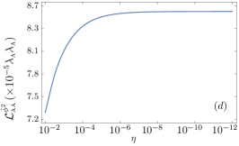
For this integrand, the limit of no cutoff, i.e, , at constant , is well-defined:
| (43) |
This integral is convergent. How the convergent limit is reached is shown numerically in Fig. 1.(d).
IV The two-detector model
The vacuum excitation probability does not provide full information about the time evolution of a pair of particle detectors coupled to the field. Indeed, to characterize more complicated effects, such as entanglement harvesting Reznik (2003); Valentini (1991); Pozas-Kerstjens and Martín-Martínez (2015), or quantum communication Blasco et al. (2015, 2016); Jonsson et al. (2015, 2014); Jonsson (2015); Martín-Martínez (2015); Landulfo (2016), the full time-evolved density matrix of two detectors coupled to the field is necessary. The detectors’ time-evolved density matrix (16) has extra terms in addition to the VEPs. Two different kinds of non-local terms, and , now appear along with their complex conjugates. To fully characterize the two detector system, we need to find explicit expressions for these terms and study the regularity of their behaviour.
As we will discuss in detail below (and as mentioned in Pozas-Kerstjens and Martín-Martínez (2015)), is the term responsible for the leading order contribution to classical correlations (or, possibly, discord) between the detectors, whereas can be thought of as responsible for the harvested entanglement from the field to the detectors, as we will discuss in section V.1. We will analyze these two terms independently in the next two subsections.
IV.1 non-local term in 3+1 dimensions
In the following, we will find for the linear and quadratic models in 3+1 dimensions.a
IV.1.1 Linear coupling,
For the linear UDW detector, the term is given by Eq. (18) when and . We also explicitly write the Wightman function in 3+1 dimensions (24), the spatial profile (32), and the switching function (33) in equation (18). The same change of coordinates as in the calculation of , shown in Eq. (34), again simplifies the calculation. This transformation yields
| (44) |
The integrals over , , the angular part of , and can be evaluated in closed form (with the same technology shown in Appendix B). As before, we follow Pozas-Kerstjens and Martín-Martínez (2015) and rewrite these integrals in terms of the dimensionless parameters as outlined in Table 1. The result is
| (45) |
which has a well-defined limit as ,
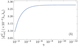
| (46) |
Not only is the integrand well-defined, but the integral is convergent as well. We show numerically how the convergent limit of is reached in Fig. 1.(b).
IV.1.2 Quadratic coupling,
In order to find , given by Eq. (18), we set and . We then substitute into Eq. (18) the quadratic two-point correlator in 3+1 dimensions (30), the spatial profile (32), and the switching function (33). As is now tradition, we will do the same change of coordinates as in the calculation of the VEPs, shown in Eq. (34). This transformation results in
| (47) |
The integrals over , , the angular part of , and can be evaluated in closed form (details in appendix B). Once again, we follow Pozas-Kerstjens and Martín-Martínez (2015) and rewrite these integrals in terms of the dimensionless quantities outlined in Table 1. The result is
| (48) |
Taking the limit as of yields
| (49) |
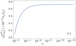
Fig. 1 (e) illustrates the behaviour as decreases of the result of numerical integration over .
IV.2 non-local term in 3+1 dimensions
In the following, we will derive and , then discuss the relevant differences between the two. We will see that has only regularizable divergences, while exhibits persistent UV divergences.
IV.2.1 Linear coupling,
For the usual linear detector, is given by Eq. (17). We substitute into Eq. (17) the Wightman function in 3+1 dimensions (24), the spatial profile (32), and the switching function (33). The integrals take a particualrly simple form under the same change of coordinates (34) as in all previous calculations. In the case of , this change of coordinates also helps to de-nest the nested time integrals. This yields
| (50) |
The integrals in , , and the angular parts of can be evaluated in closed form. This results in
| (51) |
To obtain a closed form for the integral over , we simplify by choosing to switch on the detectors simultaneously within their co-moving frame, i.e. we make the simplifying additional assumption . Under this assumption, (in dimensionless parameters as shown in 1) takes the form
| (52) |
where is the principal value of the exponential integral function defined as
| (53) |
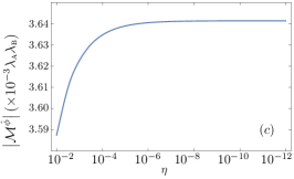
is well behaved in the UV limit. If we remove the cutoff taking the limit (i.e., ), we obtain
| (54) |
The integral is convergent, and how the limit is reached as is shown in Fig. 1.(c).
IV.2.2 Quadratic coupling,
For the quadratic detector, is given by Eq. (17). We substitute into Eq. (17) the quadratic two-point correlator in 3+1 dimensions (30), the spatial profile (32), and the switching function (33). The traditional change of coordinates shown in Eq. (34) simplifies . The result of these substitutions is
| (55) |
The integrals over , , and the angular part of can be evaluated in closed form. We can furthermore employ the simplifying assumption that the two detectors are switched on simultaneously, which results in
| (56) |
To obtain a closed from for the integral over , we operate as in the linear case and simplify by choosing to switch on the detectors simultaneously within their co-moving frame, setting . The resulting semi-closed form we write as
| (57) |
after carrying out the integral over . The details of can be found in appendix C, concretely Eq. (93).
IV.3 Divergences in the quadratic model
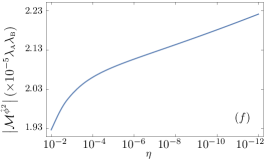
Unlike the linear model, the non-local term is not free of UV divergences, despite the fact that the detector has a smooth switching and a Gaussian spatial smearing, and despite the renormalization process that removed the single-detector divergences. Concretely, the integral in (57) is logarithmically divergent with the UV cutoff scale, as illustrated in Fig. 1.(f).
To gain insight on the logarithmic divergence in we examine the integrand , defined in the appendix equation (93).
We begin by noticing that has the limit
| (58) | ||||
Expanding in Laurent series and keeping the leading order results in the UV divergent term
| (59) |
This divergence is peculiar due to the fact that it shows up only in the two-detector model, in spite of the fact that the vacuum excitation probability for a quadratic detector is finite Hümmer et al. (2016) as discussed in section III.2. Thus, while a single quadratically coupled detector does not require additional UV regularization, a cutoff is required for certain quantities describing detector pairs, of which the term in (57) is an example.
We would like to emphasize that these are persistent UV divergences, that is, they are present regardless of the use of smooth switching functions and spatial profiles (for example, in this case we have used Gaussian functions for both). Moreover, these divergences appear after renormalization of the zero-point energy and at the same order in perturbation theory at which the single detector dynamics is regular.
V Harvesting Correlations
The analysis of the correlation terms and in both the linear and quadratic models is necessary to explore the entanglement structure of the field through particle detectors.
In this section we will study two types of correlations that the two detector models can harvest from the field vacuum: a) those measured by the mutual information, which quantifies both classical and quantum correlations adn Isaac L. Chuang (2011), and b) the negativity, which is a faithful entanglement measure for bipartite two-level systems Vidal and Werner (2002). These two types of correlation harvesting were studied for the linear model in Pozas-Kerstjens and Martín-Martínez (2015). Here we will compare these results with the predictions for the quadratic model.
V.1 Entanglement Harvesting

We consider first the harvesting of entanglement from the vacuum and we quantify it with the negativity acquired between the two (initially uncorrelated) detectors through their interactions with the field while remaining spacelike separated.
Negativity of a bipartite state is an entanglement monotone defined as the sum of the negative eigenvalues of the partial transpose of Vidal and Werner (2002):
| (60) |
where denotes the partial transpose of with respect to subsystem A.
As seen, for instance, in Pozas-Kerstjens and Martín-Martínez (2015), the negativity can be expressed in terms of the vacuum excitation probability, , of each detector and the non-local term in (57). Concretely, it is given by
| (61) |
where
| (62) |
When both detectors are identical (i.e. they have the same spatial profile, switching function, coupling strength, and detector gap), Eq. (62) becomes
| (63) |
from which we can justify the usual argument that entanglement emerges as a competition between the non-local contribution and the noise associated to the vacuum excitation probability for each detector Benni Reznik (2005); Pozas-Kerstjens and Martín-Martínez (2015).
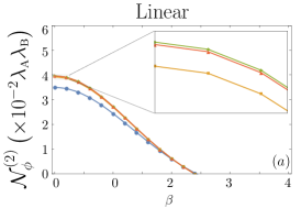
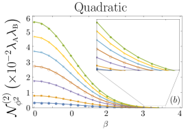
Figure 3 shows the behavior of the negativity with the spatial separation of the detectors, for the linear and quadratic case and a range of detector cutoffs.
Recall that the term is UV divergent in the quadratic model, therefore to compute a physically meaningful value for the negativity further regularization and eventual renormalization would be required. However for a fixed UV-cutoff scale, it is possible to get an estimate of the quadratic model performance to harvest entanglement relative to the linear model by computing entanglement harvesting for both models applying the same UV-cutoff scale. What is more, studying how negativity changes as we start increasing the cutoff scale will help us see how the UV divergence of impacts entanglement harvesting.
As seen in Fig. 3, the magnitude of entanglement harvesting increases linearly with the logarithm of the cutoff, which is not surprising since the two-detector quadratic model suffers a logarithmic UV divergence. This implies that there would always exist a value for the cutoff scale so that harvesting is possible at any distance, regardless of the detector gap. It would also imply that for large enough cutoff frequencies we could always ‘harvest’ more entanglement with the quadratic model than for the linear model.
One can therefore ask the following question: is there any finite value of the cutoff scale that we could take in order to give some physical meaning to the finite cutoff results?
Unlike the linear model—which has been shown to capture the fundamental features of the atom-light interaction Salton et al. (2015); Martín-Martínez et al. (2013)— the quadratic model does not have a direct comparison with something as simple as the atom-light interaction mechanism (maybe one could think of non-linear optical media Scully and Zubairy (1997), but that is perhaps a stretch). Recall, however, that we do not use the quadratic Unruh-DeWitt model to necessarily reproduce the physics of a particular experimentally motivated setup. Our motivation to explore this model is double: a) probe the field with a different model to show model independence/dependence of harvesting phenomena and b) advance towards the fermionic model (which is a quadratic model that does indeed have physical motivation) where the study of field entanglement remains still full of open questions.
The fact that this model cannot be connected with something as simple as an atom interacting with light, makes it difficult to motivate a choice of cutoff. However, if we were to take the result for a finite value of the cutoff scale seriously, and thus if we were to choose some physically motivated cutoff, we could compare the two models when such a cutoff is taken to be the Planck Frequency. In this scenario, the dimensionless cutoff parameter can be written as , where is the Planck frequency. If we consider scales for the detector gap to be commensurate with the energy of the first transition of Hydrogen s-1, then . If we set (which means that represents the case of a Hydrogen atom) the cutoff associated with the Planck time is then . We can extrapolate the results in Fig. 2 to the Planck scale. We show these results also in Fig 2, as the thin black lines. These plots illustrate the slow logarithmic nature of the divergences, which makes the study of negativity still meaningful for low energies with a quadratic detector and does not get significantly qualitatively modified even if the cutoff is transplanckian.
V.2 Harvesting Mutual Information

A way around the problems associated to the UV-divergent nature of is to look at UV-safe quantities. Namely, it is possible to find quantifiers of correlations that are, by construction, UV-safe for the quadratic model. One such figure of merit is the mutual information.
The mutual information between two detectors quantifies the amount of uncertainty about one detector that is eliminated if some information about the state of the other is revealed adn Isaac L. Chuang (2011). Thus, it constitutes a faithful measure of correlations (regardless if they are classical or quantum).
In general, for composite quantum system consisting of two subsystems A and B, the mutual information given by
| (64) |
where is the partial trace of with respect to subsystem and is the von Neumann entropy given by .
For a density matrix of the form (16), the mutual information is given by Pozas-Kerstjens and Martín-Martínez (2015)
| (65) |
where
| (66) |
Note how is not dependent on the divergent term at leading order in perturbation theory. Hence, the mutual information is finite without any further regularization. Because of this, it provides a UV-cutoff independent sense of the harvesting of correlations from the vacuum, and can also be compared with previous results for linear detectors in Pozas-Kerstjens and Martín-Martínez (2015), making it a relevant figure of merit for the comparison in this article.
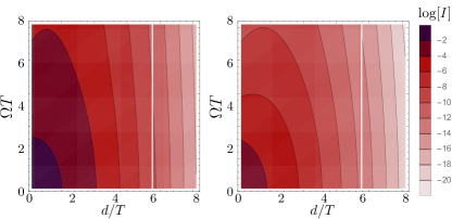
Fig. 4 shows the behavior of the Mutual information with spatial and temporal separation of the detectors for both the linear and quadratic case where the other parameters are the same as those used in Fig 2. First, we observe something that was already present in previous liteatura on linear detectors Pozas-Kerstjens and Martín-Martínez (2015): Unlike entanglement, the mutual information harvesting can be performed at any distance and detector gap, albeit less efficiently as the distance (or the detector gap) increases, a feature that comes from the fact that the detectors are harvesting classical correlations as well as quantum correlations.
From Fig. 4 we observe that the linear detector can harvest more entanglement and for further distances than the quadratic detectors. This can in turn be used to assess the scale at which the soft cutoff model introduced in the study of negativity fails to capture the behaviour of UV-safe measures of correlations: as illustrated in Fig 3, for cutoff scales that are of the order of , the linear model can harvest more entanglement than the quadratic model in the parameter region studied. This might suggest that comparison of negativity between the two models can be trusted only for cutoffs above .
VI Conclusion
We have studied further the behaviour of particle detectors quadratically coupled to scalar fields introduced in Takagi (1985, 1986) and renormalized in Hümmer et al. (2016). In particular we have focused on the case of a pair of particle detectors harvesting entanglement from a scalar field, a case previously studied only for linear detectors Benni Reznik (2005); Reznik (2003); Pozas-Kerstjens and Martín-Martínez (2015). Understanding the harvesting of correlations from quadratic couplings is a necessary step in order to compare the entanglement that can be harvested from fermionic and bosonic fields, since the former only couple to particle detectors quadratically Hümmer et al. (2016); Takagi (1985, 1986); Louko and Toussaint (2016). Our motivation to explore this model is twofold: a) probe the field with a different particle detector model to show model independence/dependence of harvesting phenomena and b) provide a model that can be compared on equal footing for bosonic and fermionic fields (for which the coupling necessarily has to be quadratic).
Perhaps the most remarkable finding of our investigation of harvesting with a quadratic detector is the appearance of a new logarithmic UV divergence at leading order in the two-detector setup. Notably, this divergence remains even when the Hamiltonian is normal-ordered, and even when the switching functions and spatial profile are smooth functions. This is in stark contrast with the linear case where smooth smearing Louko and Satz (2006) or switching Louko and Satz (2008); Satz (2007) were enough to guarantee the UV regularity of the model.
We emphasize that a single detector, at the same order in perturbation theory, does not present this kind of divergence. Curiously, the UV divergence is only present in a particular kind of term, namely that responsible for the entanglement of the two detectors. This divergence is easily parametrized via a UV cutoff.
Once this was established, analysis and comparison with the linear model can be carried out. We proceeded in two different ways. First, using negativity to study entanglement harvesting. We discussed whether a finite value of the UV cutoff scale allows for fair comparison of the entanglement harvesting ability of the quadratic and the linear couplings. Following this, we found measures of harvested correlations that are UV-safe. In particular we showed that the harvested mutual information from the field vacuum is UV safe. It therefore constitutes a better figure of merit to compare the harvesting of correlations from the vacuum without need for further regularization.
Understanding the particulars of entanglement harvesting with bosonic quadratic coupling is important in order to properly answer questions about fermionic fields where the study of field entanglement remains full of open questions Alsing et al. (2006); Martín-Martínez and León (2009, 2010a, 2010b); Fuentes et al. (2010); Bruschi et al. (2010); Martín-Martínez et al. (2010); Martín-Martínez and Fuentes (2011); Montero and Martín-Martínez (2011a, b, 2011); Montero et al. (2011); Friis et al. (2011); Brádler and Jáuregui (2012); Montero and Martín-Martínez (2012a); Friis et al. (2012); Montero and Martín-Martínez (2012b); Friis et al. (2013). A comparison of bosonic and fermionic entanglement harvesting on equal footing requires knowledge of the model-dependence entanglement harvesting, specifically the difference between linear and quadratic coupling, as the latter is necessarily present in the fermionic case. The entanglement structure of the fermionic vacuum remains an interesting open question, one we are now prepared to address using the results we have obtained.
Acknowledgements
The authors would like to thank Jose De Ramón for helpful discussions. E.M-M. and R.B.M. acknowledge the support of the Natural Sciences and Engineering Research Council of Canada NSERC programme. E.M-M also acknowledges the support of the Ontario Early Research Award.
Appendix A Calculation of the quadratic two-point function
Here we demonstrate that
| (67) |
as asserted in section II.1.1 and II.1.2, where and are defined in Eqs. (27) and (21), respectively.
The relationship between an operator and its normal ordered version is given by:
| (68) |
Using this identity, can be rewritten as
| (69) |
The first term of can be simplified. To do so, we will write the field operator as , where and are defined as
| (70) |
which satisfy the commutation relation
| (71) |
where is given by
| (72) |
Using the notation , a scalar field vacuum four point function can be rewritten as
| (73) |
where, to remove all vanishing summands, we have used that
| (74) |
together with the fact that only summands with as many as give a non-vanishing vacuum expectation.
Appendix B Convolution
In this appendix, we will find a closed form for the following integral
| (82) |
where is a positive constant, , and are non-negative constants, and are reaal constants, and .
Introducing some basic notation that we will use in this appendix, denotes the Fourier transform
| (83) |
We also introduce to denote the convolution product, defined as
| (84) |
Appendix C Quadratic Non-local Term
In this appendix we give the full-length closed expression of the integral over the variable in Eq. (56), i.e.,
| (92) |
The full expression of the integrand is
| (93) |
where Chi and Shi are the cosine and sine hyperbolic integral functions defined as
| (94) | ||||
| (95) |
and here is the Euler-Mascheroni constant, and everything is expressed in terms of dinemsnionless variables as detailed in table 1.
References
- Summers and Werner (1985) S. J. Summers and R. Werner, Physics Letters A 110, 257 (1985).
- Summers and Werner (1987) S. J. Summers and R. Werner, Journal of Mathematical Physics 28, 2440 (1987).
- Hotta (2009) M. Hotta, J. Phys. Soc. Jpn. 78, 034001 (2009).
- Hotta (2010) M. Hotta, Phys. Lett. A 374, 3416 (2010).
- Susskind et al. (1993) L. Susskind, L. Thorlacius, and J. Uglum, Phys. Rev. D 48, 3743 (1993).
- Almheiri et al. (2013) A. Almheiri, D. Marolf, J. Polchinski, and J. Sully, J. High Energy Phys. 2013, 1 (2013).
- Braunstein et al. (2013) S. L. Braunstein, S. Pirandola, and K. Życzkowski, Phys. Rev. Lett. 110, 101301 (2013).
- Salton et al. (2015) G. Salton, R. B. Mann, and N. C. Menicucci, New J. Phys. 17, 035001 (2015).
- Valentini (1991) A. Valentini, Phys. Lett. A 153, 321 (1991).
- Reznik (2003) B. Reznik, Found. Phys. 33, 167 (2003).
- Benni Reznik (2005) J. S. Benni Reznik, Alex Retzker, Phys. Rev. A (2005).
- Steeg and Menicucci (2009) G. V. Steeg and N. C. Menicucci, Phys. Rev. D 79, 044027 (2009).
- Martín-Martínez and Menicucci (2012) E. Martín-Martínez and N. C. Menicucci, Classical Quant. Grav. 29, 224003 (2012).
- Martín-Martínez and Menicucci (2014) E. Martín-Martínez and N. C. Menicucci, Classical Quant. Grav. 31, 214001 (2014).
- Martín-Martínez et al. (2016) E. Martín-Martínez, A. R. H. Smith, and D. R. Terno, Phys. Rev. D 93, 044001 (2016).
- Martín-Martínez et al. (2013) E. Martín-Martínez, E. G. Brown, and a. A. K. William Donnelly, Phys. Rev. A 88, 052310 (2013).
- Brown et al. (2014) E. G. Brown, W. Donnelly, A. Kempf, R. B. Mann, E. Martín-Martínez, and N. C. Menicucci, New J. Phys. 16, 105020 (2014).
- Olson and Ralph (2012) S. J. Olson and T. C. Ralph, Phys. Rev. A 85, 012306 (2012).
- Olson and Ralph (2011) S. J. Olson and T. C. Ralph, Phys. Rev. Lett. 106, 110404 (2011).
- Ralph and Walk (2015) T. C. Ralph and N. Walk, New Journal of Physics 17, 063008 (2015).
- Sabín et al. (2012) C. Sabín, B. Peropadre, M. del Rey, and E. Martín-Martínez, Phys. Rev. Lett. 109, 033602 (2012).
- Pozas-Kerstjens et al. (2017) A. Pozas-Kerstjens, J. Louko, and E. Martín-Martínez, Degenerate detectors are unable to harvest spacelike entanglement (To appear in Phys. Rev. D - arXiv:1703.02982, 2017).
- Pozas-Kerstjens and Martín-Martínez (2016) A. Pozas-Kerstjens and E. Martín-Martínez, Phys. Rev. D 94, 064074 (2016).
- Alsing et al. (2006) P. M. Alsing, I. Fuentes-Schuller, R. B. Mann, and T. E. Tessier, Phys. Rev. A 74, 032326 (2006).
- Martín-Martínez and León (2009) E. Martín-Martínez and J. León, Phys. Rev. A 80, 042318 (2009).
- Martín-Martínez and León (2010a) E. Martín-Martínez and J. León, Phys. Rev. A 81, 032320 (2010a).
- Martín-Martínez and León (2010b) E. Martín-Martínez and J. León, Phys. Rev. A 81, 052305 (2010b).
- Fuentes et al. (2010) I. Fuentes, R. B. Mann, E. Martín-Martínez, and S. Moradi, Phys. Rev. D 82, 045030 (2010).
- Bruschi et al. (2010) D. E. Bruschi, J. Louko, E. Martín-Martínez, A. Dragan, and I. Fuentes, Phys. Rev. A 82, 042332 (2010).
- Martín-Martínez et al. (2010) E. Martín-Martínez, L. J. Garay, and J. León, Phys. Rev. D 82, 064006 (2010).
- Martín-Martínez and Fuentes (2011) E. Martín-Martínez and I. Fuentes, Phys. Rev. A 83, 052306 (2011).
- Montero and Martín-Martínez (2011a) M. Montero and E. Martín-Martínez, Phys. Rev. A 83, 062323 (2011a).
- Montero and Martín-Martínez (2011b) M. Montero and E. Martín-Martínez, Phys. Rev. A 84, 012337 (2011b).
- Montero and Martín-Martínez (2011) M. Montero and E. Martín-Martínez, Journal of High Energy Physics 2011, 6 (2011).
- Montero et al. (2011) M. Montero, J. León, and E. Martín-Martínez, Phys. Rev. A 84, 042320 (2011).
- Friis et al. (2011) N. Friis, P. Köhler, E. Martín-Martínez, and R. A. Bertlmann, Phys. Rev. A 84, 062111 (2011).
- Brádler and Jáuregui (2012) K. Brádler and R. Jáuregui, Phys. Rev. A 85, 016301 (2012).
- Montero and Martín-Martínez (2012a) M. Montero and E. Martín-Martínez, Phys. Rev. A 85, 016302 (2012a).
- Friis et al. (2012) N. Friis, A. R. Lee, D. E. Bruschi, and J. Louko, Phys. Rev. D 85, 025012 (2012).
- Montero and Martín-Martínez (2012b) M. Montero and E. Martín-Martínez, Phys. Rev. A 85, 024301 (2012b).
- Friis et al. (2013) N. Friis, A. R. Lee, and D. E. Bruschi, Phys. Rev. A 87, 022338 (2013).
- Iyer and Kumar (1980) B. R. Iyer and A. Kumar, Journal of Physics A: Mathematical and General 13, 469 (1980).
- Unruh (1976) W. G. Unruh, Phys. Rev. D 14, 870 (1976).
- Takagi (1985) S. Takagi, Prog. Theor. Phys. 74, 501 (1985).
- Takagi (1986) S. Takagi, Prog. Theor. Phys. Supp. 88, 1 (1986).
- Hümmer et al. (2016) D. Hümmer, E. Martín-Martínez, and A. Kempf, Phys. Rev. D 93, 024019 (2016).
- DeWitt (1979) S. DeWitt, General Relativity: An Einstein Centenary Survey, edited by S. W. Hawking and W. Israel (Cambridge University Press, 1979) p. 680.
- Hinton (1984) K. J. Hinton, Classical Quant. Grav. 1, 27 (1984).
- Louko and Satz (2008) J. Louko and A. Satz, Classical Quant. Grav. 25, 055012 (2008).
- Louko and Satz (2006) J. Louko and A. Satz, Classical Quant. Grav. 23, 6321 (2006).
- Satz (2007) A. Satz, Classical Quant. Grav. 24, 1719 (2007).
- Pozas-Kerstjens and Martín-Martínez (2015) A. Pozas-Kerstjens and E. Martín-Martínez, Phys. Rev. D 92, 064042 (2015).
- Jonsson et al. (2015) R. H. Jonsson, E. Martín-Martínez, and A. Kempf, Phys. Rev. Lett. 114, 110505 (2015).
- Blasco et al. (2015) A. Blasco, L. J. Garay, M. Martín-Benito, and E. Martín-Martínez, Phys. Rev. Lett. 114, 141103 (2015).
- Martín-Martínez and Louko (2015) E. Martín-Martínez and J. Louko, Phys. Rev. Lett. 115, 031301 (2015).
- Martín-Martínez (2015) E. Martín-Martínez, Phys. Rev. D 92, 104019 (2015).
- Blasco et al. (2016) A. Blasco, L. J. Garay, M. Martín-Benito, and E. Martín-Martínez, Phys. Rev. D 93, 024055 (2016).
- Jonsson et al. (2014) R. H. Jonsson, E. Martín-Martínez, and A. Kempf, Phys. Rev. A 89, 022330 (2014).
- Jonsson (2015) R. H. Jonsson, arXiv:1512.05065 (2015).
- Landulfo (2016) A. G. S. Landulfo, Phys. Rev. D 93, 104019 (2016).
- adn Isaac L. Chuang (2011) M. A. N. adn Isaac L. Chuang, Quantum Computation and Quantum Information (Cambridge University Press, 2011).
- Vidal and Werner (2002) G. Vidal and R. F. Werner, Phys. Rev. A 65, 032314 (2002).
- Scully and Zubairy (1997) M. O. Scully and M. S. Zubairy, Quantum Optics (Cambridge University Press, 1997).
- Louko and Toussaint (2016) J. Louko and V. Toussaint, Phys. Rev. D 94, 064027 (2016).