Configurational entropy measurements in extremely supercooled liquids that break the glass ceiling

Abstract

Liquids relax extremely slowly upon approaching the glass state. One explanation is that an entropy crisis, due to the rarefaction of available states, makes it increasingly arduous to reach equilibrium in that regime. Validating this scenario is challenging, because experiments offer limited resolution, while numerical studies lag more than eight orders of magnitude behind experimentally-relevant timescales. In this work we not only close the colossal gap between experiments and simulations but manage to create in-silico configurations that have no experimental analog yet. Deploying a range of computational tools, we obtain four estimates of their configurational entropy. These measurements consistently confirm that the steep entropy decrease observed in experiments is also found in simulations, even beyond the experimental glass transition. Our numerical results thus extend the new observational window into the physics of glasses and reinforce the relevance of an entropy crisis for understanding their formation.

Introduction– In his landmark 1948 paper, Kauzmann gathered experimental data for several glass-forming liquids and found that they all showed a steep decrease of their equilibrium configurational entropy upon lowering temperature towards their glass transition Kauzmann (1948). Theoretically, the nature of a thermodynamic glass transition associated with a vanishing configurational entropy is well-understood at the mean-field level Kirkpatrick and Thirumalai (1987); Kirkpatrick and Wolynes (1987); Charbonneau et al. (2014a), suggesting that glass formation is accompanied by a rarefaction of available disordered states Berthier and Biroli (2011). Its pertinence beyond the mean-field framework, however, remains controversial Kirkpatrick et al. (1989); Stillinger (1988); Garrahan and Chandler (2003); Berthier and Biroli (2011). In particular, it is still not known whether such entropy reduction is the core explanation for glass formation. Experimental measurements are carried out over too limited a temperature range, within boundaries that have remained essentially unchanged since Kauzmann’s work and thus form a solid glass ceiling. In addition, experimental determinations of the configurational entropy are marred by approximations that influence their physical interpretation Dyre (2006); Wyart (2010); Rabochiy et al. (2013a). Computer simulations can potentially provide more precise estimates Sciortino et al. (1999); Berthier and Coslovich (2014), but have so far been restricted to a temperature range that is not experimentally relevant.

Can the debate over the role of configurational entropy ever be settled? At first sight, closure appears unlikely for two main reasons. (i) Measuring the configurational entropy below the experimental glass transition seems logically impossible, because experiments are constrained by their own duration, which fixes an upper limit to the accessible thermalization timescale, $\tau$. Specifically, $\tau/\tau_{0}\sim 10^{13}$ for molecules Petzold et al. (2013) (where the relaxation time at the onset temperature is $\tau_{0}\approx 10^{-10}{\rm s}$) and $\tau/\tau_{0}\sim 10^{5}$ for colloids Brambilla et al. (2009) (where $\tau_{0}\approx 10^{-1}{\rm s}$). The situation for computer simulations is even worse. Current approaches access at most $\tau/\tau_{0}\sim 10^{5}$, which is eight orders of magnitude behind molecular liquid experiments, and numerical progress has been slow. The two to three decades gained over the past 35 years Barrat et al. (1990); Kob and Andersen (1994); Brambilla et al. (2009) are mostly thanks to hardware improvements. At this pace, another century would be needed before simulations attain experimentally-relevant conditions. The glass ceiling thus appears unbreakable. (ii) There is a fundamental methodological ambiguity as to which configurational entropy should be measured in order to match theoretical calculations. Qualitatively, the configurational entropy is defined by subtracting vibrational contributions from the total entropy Kauzmann (1948); Martinez and Angell (2001); Sciortino et al. (1999). What is specifically meant by “vibrations” in amorphous solids, however, is ill-defined in general Berthier and Biroli (2011) and difficult to measure in practice Kauzmann (1948); Berthier and Coslovich (2014). Hence consistently determining the configurational entropy is in itself a difficult challenge, that may be underestimated in the literature.

Here, we solve both of these major problems at once. First, we take advantage of the flexibility offered by computer simulations to dramatically accelerate the equilibrium sampling of configuration space Grigera and Parisi (2001); Berthier et al. (2016a); Ninarello et al. (2017a). Namely, we use a system optimized for the nonlocal swap Monte Carlo (MC) algorithm, which enables its extremely fast thermalization. We establish that this approach surpasses any current alternative, and even experimental protocols. Second, we measure four proxies for the configurational entropy by deploying state-of-the-art computational tools to characterize in-silico configurations that are more deeply equilibrated than their experimental analogs Angelani and Foffi (2007); Berthier et al. (2016a); Berthier and Coslovich (2014); Berthier et al. (2016b) and obtain consistent results that have a clear physical interpretation. By combining these developments for a realistic model glass-former, we shift computer simulations from lagging eight decades behind experiments to exploring novel territory in glass physics. In particular, our measurements validate Kauzmann’s observations that the configurational entropy decreases steeply towards the glass temperature, and extend these observations to a regime previously inaccessible.

Figure 1: Breaking the glass ceiling: thermalization beyond the experimental glass transition. (A) Structural relaxation time, $\tau$, for both standard and accelerated swap MC dynamics as a function of the reduced pressure of a polydisperse hard sphere model, where $\tau$ is obtained from the decay of the self-intermediate scattering function at a wavenumber $k=5.25$. The onset of slow dynamics occurs at $Z_{0}\approx 18$, and the mode-coupling crossover at $Z_{c}\approx 23.5$. Times are rescaled by $\tau_{0}=\tau(Z_{0})$ for standard MC. The current limit of colloidal ($\tau/\tau_{0}=10^{5}$) and molecular ($\tau/\tau_{0}=10^{13}$) experiments are indicated by vertical bands (this uncertainty stems from the extrapolation scheme), showing that swap MC breaks the glass ceiling. Static structure factor for $Z=18.8\approx Z_{0}$ ($\phi=0.568$) and $Z=33.2$ ($\phi=0.640$) for (B) all particles (C) the 40% particles with the smallest diameter. (D, E) show typical snapshots for these two state points, where the smallest particles are highlighted in blue.

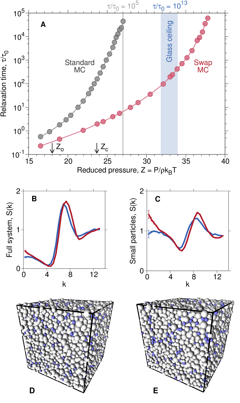
Results– We simulate a three-dimensional polydisperse mixture of hard spheres, as in Berthier et al. (2016a), which is a good model for colloids used in experiments Pusey and Van Megen (1986); Brambilla et al. (2009). We show in Appendix I that our methods and conclusions also apply to particles with soft and more complex interactions. We control the volume fraction $\phi$, and measure pressure $P$ to report the (unitless) reduced pressure, $Z=P/(\rho k_{B}T)$, where $\rho$ is the number density, and $k_{B}T$ the thermal energy. This natural control variable for hard spheres plays a role akin to the inverse temperature in thermal liquids Berthier and Witten (2009). Detailed information about the simulations is provided in Appendices A, B, and C. Swap MC complements standard translational MC moves with nonlocal moves that exchange randomly-chosen pairs of particles, ensuring equilibrium sampling. Detailed tests of thermalization of all glassy degrees of freedom are reported in Appendix D, see also Ref. Ninarello et al. (2017a). We demonstrate the extreme speedup actually achieved by swap MC for this model in Fig. 1, in which the structural relaxation time $\tau$ for both MC sampling methods is reported as the system approaches its glass transition. Note that the rapid increase of $\tau$ in standard MC simulations resembles the fragile super-Arrhenius behavior of standard glass-formers Berthier and Biroli (2011). We can only indirectly assess fragility beyond the reported numerical regime, which we estimated to be $m\approx 50$. We have fitted several empirical forms to our measurements, which thermalize up to $Z\approx 27$, to estimate the experimental glass transition at $\tau/\tau_{0}=10^{13}$ (see Appendix E). Use of various fits reflects the well-known uncertainties associated with the empirical description of data measured over a large dynamical range Stickel et al. (1995). The fits give consistent locations for the glass ceiling, $Z_{\mathrm{g}}\approx 32$-34, as highlighted in Fig. 1. Remarkably, this dramatic slowdown is completely bypassed by swap MC sampling, which thermalizes the system up to $Z\approx 38>Z_{\mathrm{g}}$. Even most conservative extrapolation indicates that we access a dynamical range that is broader than in experiments. Meanwhile, the two-point structure barely budges (see Figs. 1B-C), which is a telltale sign of glassiness Berthier and Biroli (2011) and a confirmation that both crystallization and more subtle fractionation effects are absent. Visual inspection of particle configurations further confirm these conclusions (see, e.g., Figs. 1D-E). We are therefore in the unique position of studying at equilibrium a homogeneous supercooled liquid beyond the experimental glass ceiling.

Figure 2: Numerical procedures leading to the four estimates of the configurational entropy. (A) Method 1: The Frenkel-Ladd method to obtain the vibrational entropy $s_{\mathrm{vib}}$ performs a thermodynamic integration of the mean-squared distance $\delta r^{2}$ between a reference equilibrium configuration and a copy of the system constrained by a harmonic potential of strength $\alpha$. The integration is carried out from $\alpha_{\rm max}$, for which the system behaves as an Einstein solid (indicated by the dashed line $\delta r^{2}=3/(2\alpha)$) to $\alpha_{\rm min}$, for which particles are trapped by their own cages on the vibrational time scale. (B) Method 2: The numerically-determined Franz-Parisi potential $V(Q)$ is used to measure the configurational entropy as $s_{\rm conf}=V(Q_{\rm high}=0.8)-V(Q_{\rm low}\approx 0.05)$. (C) Method 3: The evolution of the overlap $Q$ with the biasing field $\varepsilon$ reveals a first-order jump at a value $\varepsilon^{\star}$ for which $Q=1/2$ (dashed line). Then, $s_{\rm conf}=\varepsilon^{\star}(Q_{\rm high}-Q_{\rm low})$. (D) Method 4: The decay of the cavity overlap correlation function $Q_{\rm PTS}(R)$ with cavity radius, $R$, defines the point-to-set correlation length $\xi_{\mathrm{PTS}}\propto s_{\mathrm{conf}}^{-1/(d-\theta)}$.

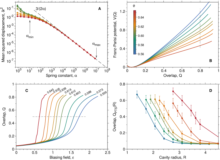
We then turn to measuring the configurational entropy, $s_{\rm conf}$, in these extremely supercooled configurations. The numerical procedures leading to the four estimates of $s_{\rm conf}$ are shown in Fig. 2. Further details are provided in Appendices F, G, and H. In Method 1, we determine the configurational entropy from its most conventional definition, $s_{\mathrm{conf}}=s_{\mathrm{tot}}-s_{\mathrm{vib}}$, as used in many experimental and simulation studies Kauzmann (1948); Martinez and Angell (2001); Sciortino et al. (1999); Angelani and Foffi (2007). The total entropy of the equilibrium fluid, $s_{\mathrm{tot}}$, is measured by thermodynamic integration from the dilute ideal gas limit to the target volume fraction, while the vibrational contribution, $s_{\mathrm{vib}}$, is measured by Frenkel-Ladd thermodynamic integration Angelani and Foffi (2007); Frenkel and Ladd (1984). The latter integration is over the amplitude of the Hookean constant, $\alpha$, of a spring that constrains each particle to reside close to the position of a quenched reference equilibrium configuration. This requires estimating the mean-squared distance $\delta r^{2}$ between the reference and constrained systems over a broad range of $\alpha$ values, as illustrated in Fig. 2(A). In continuously polydisperse systems, special care is also needed to account for the mixing contribution to the total entropy, because this contribution formally diverges Frenkel (2014); Ozawa and Berthier (2017). The mixing entropy is thus determined from an independent, additional set of simulations Ozawa and Berthier (2017) (see Appendix F). Method 1 is equivalent to partitioning configuration space into basins of attraction of inherent structures Stillinger (1988). The resulting estimate of the configurational entropy thus counts the number of energy minima Stillinger and Weber (1985); Sciortino et al. (1999), which presumably overestimates the number of relevant basins in the free energy landscape Biroli and Monasson (2000).

Methods 2 and 3 are both based on the Franz-Parisi theoretical construction Franz and Parisi (1997), which expresses the equilibrium free energy of the liquid, $V(Q)$, in terms of a global order parameter, the overlap $Q$. The overlap between two configurations is defined as $Q=N^{-1}\sum_{i,j}\theta(a-|{\bf r}_{1,i}-{\bf r}_{2,j}|)$, where $\theta(x)$ is the Heaviside function, ${\bf r}_{1,i}$ and ${\bf r}_{2,j}$ are the positions of particle $i$ and $j$ within configuration 1 and 2, and $a$ is a fraction of the average particle diameter. By definition, $Q$ quantifies the similarity between the coarse-grained density profiles of two configurations. To compute $V(Q)$, we introduce a coupling between a quenched reference equilibrium configuration and a copy of the system through a field $\varepsilon$ conjugate to $Q$ Franz and Parisi (1997); Berthier and Coslovich (2014); $\varepsilon$ constrains the collective density profile, whereas $\alpha$ in Method 1 constrains single-particle displacements. We define $V(Q)=-\lim_{\varepsilon\to 0}\left[\frac{T}{N}\ln P(Q)\right]$, where $P(Q)$ is the equilibrium probability distribution of the overlap for a given reference configuration, and brackets denote averaging over these configurations. In Method 2, we follow Berthier and Coslovich (2014) and use the free-energy difference $s_{\rm conf}=V(Q_{\rm high})-V(Q_{\rm low})$ between the global minimum at $Q_{\rm low}\approx 0.05$ and its value at $Q_{\rm high}=0.8$ to obtain an estimate of $s_{\rm conf}$ that is closest to its theoretical definition, see Fig. 2(B). Importantly, this estimate only exists for sufficiently supercooled states, for which $Q_{\rm high}$ can be defined Berthier and Coslovich (2014). For the present system, this happens close to the mode-coupling crossover, $Z_{c}$. In Method 3, we determine the value of the biasing $\varepsilon$ needed to ‘tilt’ the potential $V(Q)$, so that a first-order phase transition, at which $Q$ jumps from $Q_{\rm low}$ to $Q_{\rm high}$, takes place as illustrated in Fig. 2(C). We use the maximum variance of the overlap fluctuations to measure $\varepsilon^{\star}$ for each volume fraction studied. In practice, this is equivalent to determining the biasing field at which the overlap reaches $Q=1/2$, see Fig. 2(C).

Method 4 builds on the physical idea that the decrease of the configurational entropy is directly responsible for the growth of spatial correlations quantified by the point-to-set correlation length, $\xi_{\rm PTS}$ Adam and Gibbs (1965); Bouchaud and Biroli (2004); Biroli et al. (2008). Following what is becoming common practice Biroli et al. (2008); Berthier et al. (2016b), we measure $\xi_{\rm PTS}$ by pinning the position of particles outside a spherical cavity of radius $R$, equilibrating the liquid within it, and measuring the evolution of the overlap between interior configurations, $Q_{\rm PTS}(R)$, with the cavity radius $R$, as shown in Fig. 2(D). The decay of $Q_{\rm PTS}(R)$ is controlled by $\xi_{\rm PTS}$, and the variance of the overlap fluctuations also presents a maximum Berthier et al. (2016b) very close to $\xi_{\rm PTS}$. Physically, $\xi_{\rm PTS}$ thus represents the cavity size above which the system starts to explore a significant number of distinct states. With minimal hypothesis Bouchaud and Biroli (2004), it can be connected to the configurational entropy through $s_{\rm conf}\propto\xi_{\rm PTS}^{-(d-\theta)}$, with an unknown exponent $\theta\leq(d-1)$. Various values of $\theta$ have been proposed, including $\theta=2$ from saturating the inequality and $\theta=3/2$ from a wetting argument Kirkpatrick et al. (1989); Lubchenko (2015). However, our measurements are consistent with both of these values and thus cannot unambiguously distinguish one proposal from the other.

Figure 3: Convergent measurements of the four estimates of the configurational entropy beyond the glass ceiling. $s_{\mathrm{conf}}$ is plotted as a function of $1/Z\propto T/P$, which is equivalent to the classic Kauzmann plot. All measurements indicate a steep decrease of $s_{\rm conf}$ that continues as the experimental glass ceiling is crossed. The point-to-set estimates are normalized with $\xi_{0}=2.0$ for $\theta=2$ and $\xi_{0}^{\prime}=2.1$ for $\theta=3/2$, respectively, to match the Franz-Parisi estimates at the start of the low-temperature regime, $1/Z=0.04\approx 1/Z_{\rm c}$. The dashed line is an extrapolation based on $s_{\mathrm{tot}}-s_{\mathrm{vib}}$ (see Appendix F). Inset: typical overlap profiles measured in a finite cavity of radius $R=3.46$, with colors coding for the overlap value from low (white) to large (black). Overlap fluctuations are uncorrelated around the onset but become strongly correlated over the entire cavity at the largest pressure shown.

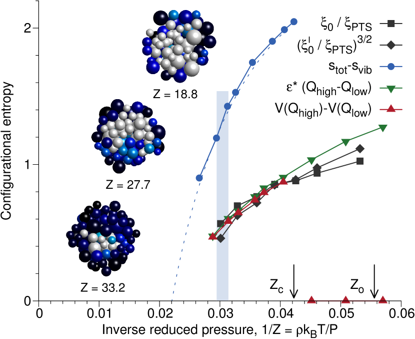
We gather the four estimates of the configurational entropy in Fig. 3 to produce a plot akin to the original 1948 Kauzmann representation of $s_{\rm conf}(T)$ Kauzmann (1948). Although in the high-temperature liquid the configurational entropy is not sensibly defined Berthier and Coslovich (2014), three of the four measures can still be estimated. Note that only this regime was accessible in earlier simulations Sciortino et al. (1999); Angelani and Foffi (2007); Berthier and Coslovich (2014). In the more relevant low-temperature regime, our main finding is that the important conceptual and technical differences between the four methods nevertheless result in qualitatively consistent results. In particular, the three estimates (Methods 2-4) that closely follow the theoretical definition of the configurational entropy provide numerically indistinguishable results at low temperatures. The conventional estimate of the entropy (Method 1) is larger, as expected Biroli and Monasson (2000), but its temperature evolution remains qualitatively consistent with the other methods. All our estimates of $s_{\rm conf}$ thus exhibit a steep decrease as $Z$ increases towards the glass phase, which is consistent with the seemingly fragile behavior of the model in Fig. 1. Although a quantitative extrapolation is hard to control, our measurements robustly suggest that $s_{\rm conf}$ may vanish near $Z\approx 1/0.022\approx 45$. We thus conclude that even for a simple glass-forming system equilibrated deeper in the landscape than any previously studied material, the trend discovered 70 years ago by Kauzmann is confirmed when more precise estimates of $s_{\rm conf}$ are adopted, and persists even below the experimental glass temperature.

We further show in Appendix I that similar observations can be performed for a model with a continuous pair potential, suggesting our methodological progress and physical conclusions are not restricted to hard spheres, and likely apply more generally. Note that while continuous polydisperse distributions are commonplace in colloidal suspensions, a molecular liquid with a sufficiently large number of components to approximate a continuous size distribution has yet to be considered.

Discussion– Our point-to-set measurements go beyond Kauzmann’s observation by establishing that the decrease in $s_{\rm conf}$ is accompanied by an increase of static spatial correlations as the glass ceiling is crossed. This result reinforces a recent experimental report based on non-linear dielectric measurements Albert et al. (2016). In absolute value, the measured static length scale at the experimental glass transition appears somewhat smaller than previous estimates based on dynamical correlations Rabochiy et al. (2013b); Berthier et al. (2005), but remains compatible with the modest growth expected from general arguments based on thermally activated scaling Kirkpatrick et al. (1989); Bouchaud and Biroli (2004); Lubchenko (2015) and decorrelation between static and dynamical length scales Charbonneau and Tarjus (2013). Our particle-based resolution of such correlations further provides a direct visualization of the spatial profile of the overlap within a spherical cavity (see insets in Fig. 3). In particular, within a cavity comprising about 200 particles, the positions of particles freely fluctuate near the onset pressure, but become strongly correlated over the entire cavity for the largest pressure shown. The spatial extent of static correlations is thus directly revealed.

The important methodological advances achieved here regarding the thermalization of supercooled liquids and the measurement of configurational entropy therefore support a thermodynamic view of the glass formation based on the rarefaction of metastable state accompanied by growing static correlations that is devoid of the experimental ambiguities and that extends to a temperature regime that has never been explored before.

Appendix A Model

We study a three-dimensional hard-sphere model, for which the pair interaction is zero for non-overlapping particles and infinite otherwise. Systems have a continuous size polydispersity, with particle diameters $\sigma$ randomly drawn from the distribution $f(\sigma)=A\sigma^{-3}$, with $\sigma\in[\sigma_{\rm min},\sigma_{\rm max}]$ with normalization constant $A$. Our model is the same as that studied in Ref. Berthier et al. (2016a), with a measure of size polydispersity $\Delta=\sqrt{\overline{\sigma^{2}}-\overline{\sigma}^{2}}/\overline{\sigma}$, where $\overline{\cdots}=\int d\sigma f(\sigma)(\cdots)$, of $\Delta=23\%$, and $\sigma_{\rm min}/\sigma_{\rm max}=0.4492$. The average diameter, $\overline{\sigma}$, defines the unit of length. We simulate systems composed of $N$ particles in a cubic cell of volume $V$ under periodic boundary conditions Allen and Tildesley (1989). Depending on the chosen method to estimate the configurational entropy (see Appendix F), we simulate systems with either $N=1000$, $8000$ (Method 1) or $N=300$ (Method 2 and 3). Cavities for Method 4 are carved from bulk configurations with $N=8000$. The relaxation times shown in Figure 1A are obtained from samples with $N=1000$. Given these parameters, the system is then uniquely characterized by its volume fraction $\phi=\pi N\overline{\sigma^{3}}/(6V)$, and we frequently report the data using the reduced pressure $Z=P/(\rho k_{\rm B}T)$, where $\rho$, $k_{\rm B}$, and $T$ are the number density, Boltzmann constant and temperature, respectively. Without loss of generality, we set $k_{B}$ and $T=1/\beta$ to unity. The pressure $P$ is calculated from the contact value of the pair correlation function properly scaled for a polydisperse system Santos et al. (2005).

Appendix B Methods

To obtain equilibrium fluid configurations deep in the glassy regime, we perform Monte-Carlo (MC) simulations with both translational displacements and non-local particle swaps Berthier et al. (2016a); Gazzillo and Pastore (1989); Sindzingre et al. (1989); Santen and Krauth (2001); Pronk and Frenkel (2004); Grigera and Parisi (2001); Frenkel and Smit (2001); Brumer and Reichman (2004); Gutiérrez et al. (2015). The two types of moves are selected randomly: with probability $0.8$ we attempt a translational displacement, and with probability $0.2$ we attempt a swap. Translational displacements are uniformly drawn over a cube of side $0.115$. For swaps, two randomly selected particles exchange diameter. In both cases, proposed moves are accepted if no overlap is created. Following Ref. Ninarello et al. (2017a), we also immediately reject swaps between particles whose diameters differ by more than $0.2$.

We measure the equilibrium relaxation time $\tau$ both with and without the swap moves from the time-decay of the self-intermediate scattering function, $F_{s}(k,\tau)=1/e$, where $k=5.25$ is the wavenumber chosen slightly below the first maximum of the static structure factor. Note that the particles’ diameters can change during a swap MC simulation, but their trajectories are continuous. Relaxation times are measured in units of MC sweeps, comprising $N$ MC moves, irrespective of their type.

Thermalized systems at each state point are obtained in the same way for both standard and swap MC dynamics. We measure the relaxation time $\tau$ and ensure that for each state point simulations of a total duration of at least $100\tau$ can be performed. We also check for the presence of aging effects in time correlation functions, and we measure the static structure factor, the pair correlation function and the equation of state over long simulations, paying attention to any temporal drift that could signal either improper thermalization, incipient crystallization or demixing of particles with distinct sizes. Selected results for the evolution of the structure factor with volume fraction are presented in Figs. 1B-C. Over the extreme range of densities shown here, the static structure evolves very little. Similarly, a very modest evolution is seen when the partial structure factor of the smallest particles is measured. A large increase of the low-$k$ value of these quantities, or the emergence of discrete peaks would signal that demixing or crystallization is taking place. In fact, we have found that measuring the relaxation time for the swap simulation is the most sensitive test of thermalization, because purely static observables may appear thermalized over long simulation times, whereas the system is in fact nearly arrested in a glass state within which sampling is inefficient.

We introduce two dynamical reference states: (i) the onset of slow dynamics at $\phi_{0}\approx 0.56$ ($Z_{0}\approx 18$), above which the time decay of correlation functions is non-exponential Sastry et al. (1998), and (ii) the mode-coupling crossover $\phi_{\rm c}\approx 0.598$ ($Z_{\rm c}\approx 23.5$), at which a power-law fit extrapolates a divergence of the relaxation times Berthier et al. (2016a). Note that these particular definitions are not unique Charbonneau et al. (2014b), but are sufficiently accurate for our purposes, where these values are simply used for qualitative reference.

Appendix C Equation of state

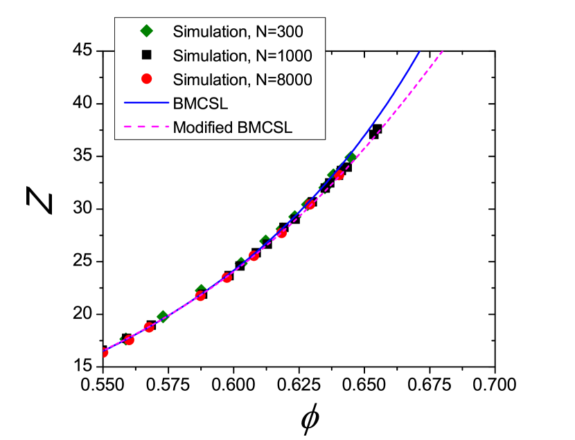
We report in Fig. S1 the equilibrium equation of state, $Z=Z(\phi)$ (from Ref. Berthier et al. (2016a)), of the system under study, thus enabling a translation of the reported results from $Z$ to $\phi$. The specific data points used in the four measurements of the configurational entropy are also presented in Tab. 1, 2, and  3.

Figure S1: Equation of state $Z=Z(\phi)$ for the hard-sphere system studied in this work. The solid line is the empirical expression for the equation of state from Refs. Boublík (1970); Mansoori et al. (1971), BMCSL, which describes our data well, except at very large volume fractions, where it slightly overestimates $Z$. A modified version of BMCSL Berthier et al. (2016c) is given by the dashed line.

$Z$	17.6	19.8	22.3	24.8	27.0	28.1	30.4	32.0	34.9
$\phi$	0.559	0.573	0.588	0.603	0.612	0.619	0.628	0.635	0.645

Table 1: Data points for $N=300$ used in the Franz-Parisi construction (Methods 2 and 3).

$Z$	23.7	24.6	25.8	28.3	30.7	32.0	34.0	37.6
$\phi$	0.598	0.602	0.609	0.619	0.630	0.635	0.643	0.655

Table 2: Data points for $N=1000$ used in the thermodynamic integrations (Methods 1).

$Z$	18.8	21.7	23.5	25.6	27.7	30.4	33.2
$\phi$	0.568	0.587	0.597	0.608	0.618	0.629	0.640

Table 3: Data points for $N=8000$ used in the thermodynamic integration computations (Methods 1) and the point-to-set correlation (Method 4).

Appendix D Equilibration

Figure S2: Panel A: Collective overlap time correlation function $Q_{c}(t)$ for several packing fractions (from left to right, $\phi=0.568$, 0.609, 0.640, 0.655). Panel B: Probability of losing all but one neighbor $P_{b}^{(1)}(t)$ as a function of time for the same packing fractions as in panel A.

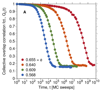
In this section, we present evidence that strongly supports the equilibration of our samples. In addition to the tests mentioned in the Methods section of the main text, we also verified the equivalence of derivative and fluctuation expressions for the compressibility, which is a well-known equilibration check Vasisht et al. (2011). The validity of this sum rule is, however, not necessarily a strong test of equilibration, because it may appear to hold within the noise of the data, even in systems that are not fully equilibrated. A more stringent test of equilibration is to show that all the slow degrees of freedom relax within the observation time. In a structural glass former, the relevant slow degrees of freedom are those associated with collective density fluctuations and with cage breaking. To measure the decorrelation of the former, we introduce the time-dependent collective overlap function

$$Q_{c}(t)=N^{-1}\sum_{i}\sum_{j}\Theta(a-|\vec{r}_{i}(t)-\vec{r}_{j}(0)|),$$ (1)

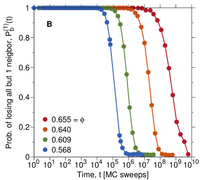
where $\Theta(x)$ is the Heaviside function and $a=0.346$. The decay of $Q_{c}(t)$ quantifies the relaxation of density fluctuations up to a coarse-graining length $a$. In order to analyze cage breaking, here defined as the process of a particle losing some of its neighbors within a given time span Shiba et al. (2012), the following procedure is employed. First, we identify the neighbors of a particle by a radical Voronoi tessellation obtained using the Voro++ package Rycroft (2009). Note that the average number of neighbors measured for our densest states is about 14. Second, we measure the probability, $P_{b}^{(k)}(t)$, that a particle has changed all but $k$ of its initial neighbors after a time $t$. For small $k$, the decay of $P_{b}^{(k)}(t)$ provides evidence for the complete restructuring of the cages and ensures that a pseudo-molecular structure is not found in the fluid.

Representative results of $Q_{c}(t)$ and $P_{b}^{(1)}(t)$, measured in swap MC simulations of the $N=1000$ system, are shown in Fig. S2. All these functions decay to trivial plateaus within our simulations, with the possible, albeit mild, exception of the data point at the highest packing fraction. We also note that although the cage breaking probability decays more slowly than $Q_{c}(t)$, the associated relaxation times grow in a similar way. Our simulations thus pass this very stringent equilibration test, in addition to those already mentioned in the main text and in Ref. Berthier et al. (2016a). For the soft polydisperse model studied in Sec. I of the SM, a similar analysis was performed in Ref. Ninarello et al. (2017b).

Appendix E Locating the glass ceiling

In the context of this work, we refer to the typical relaxation time measured at the laboratory glass transition (at which, conventionally, $\tau/\tau_{0}=10^{13}$ Petzold et al. (2013)) as the glass ceiling, $Z_{\rm g}$. Because standard MC dynamics can only access relaxation times at most of order $\tau/\tau_{0}=10^{5}$, where $\tau_{0}=10^{4}$ MC sweeps is the value of $\tau$ at the onset of slow dynamics, our dynamical data have to be extrapolated to locate this ceiling. We fit measured relaxation times to various functional forms up to $\tau/\tau_{0}\leq 10^{5}$, and then extrapolate up to the vicinity of the glass ceiling. In an effort to obtain an estimate as unbiased as possible, we consider a range of possible functional forms Berthier and Witten (2009); Berthier and Biroli (2011), as detailed below. We present in Fig. S3 the result of this exercise. In particular, note that whereas extrapolating the location of a putative divergence of $\tau$ is extremely delicate, extrapolating the location of the glass ceiling is in fact rather well-controlled.

Figure S3: The measured relaxation time, $\tau$, (symbols) is fitted to the VFT form, Eq. (2), with exponents $\delta=1$ and $\delta=2$, the parabolic law, Eq. (3), and the Arrhenius law, Eq. (4). The first three fits provide a good description of the data, and are used to locate the glass ceiling at $\tau/\tau_{0}=10^{13}$ that is used in the main text.

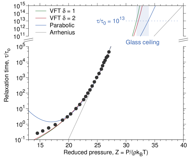
The first functional form is the Vogel-Fulcher-Tammann (VFT) expression

$$\tau=\tau_{\infty}\exp\left[\frac{A}{(Z_{\rm vft}-Z)^{\delta}}\right],$$ (2)

where $\tau_{\infty}$, $A$, the exponent $\delta$ and the critical pressure $Z_{\rm vft}$ are free parameters. Whereas $\delta=1$ is traditionally used, more recent experimental and numerical studies Brambilla et al. (2009); Berthier and Witten (2009) favor $\delta=2$. In Fig. S3 we consider both. As noted before Berthier et al. (2016a), the fit with $\delta=1$ yields a critical pressure $Z_{\rm vft}\approx 38$ that falls within the range in which swap MC sampling equilibrates. Although the resulting fit is good over the range covered by standard MC dynamics, it overestimates the growth of the relaxation time beyond that range, which undermines the very logic behind the proposed scaling form. When $\delta=2$ is imposed the fit is still very good, but we now obtain $Z_{\rm vft}\approx 45$, which is at least beyond the equilibrium range accessible with the swap method. Although this fit provides a more consistent description of the dynamical data, resolving one form from the other is beyond the scope of the current study.

The second functional form is the parabolic law proposed by Elmatad et al. Elmatad et al. (2009); Isobe et al. (2016) in the context of facilitated models,

$$\tau=\tau_{\infty}\exp\left[A(Z-Z_{0})^{2}\right],$$ (3)

where $Z_{0}=17$ is around the onset of slow dynamics and the fit is made over the range $Z>Z_{0}$. In contrast to the VFT law, this parabolic expression does not invoke a divergence of the relaxation time at any finite pressure; $\tau$ only diverges when $Z$ also diverges. Note that because $Z\propto 1/T$, this form is equivalent to fitting the relaxation time of a supercooled liquid without any finite-temperature divergence Berthier and Witten (2009). As a result this expression necessarily provides a less divergent extrapolation of the relaxation time at large pressures, but still accounts well for the curvature, i.e., the fragility, of the measured dynamical data. The leading order at large $Z$, $\tau\propto\exp[AZ^{2}]$, indeed grows faster than the Arrhenius law. Like the VFT form, this fit is quite good over the measured range of relaxation times, see Fig. S3.

For completeness, we also include a simple Arrhenius fit to the high-$Z$ portion of the equilibrium data

$$\tau=\tau_{\infty}\exp[{A}{Z}].$$ (4)

We find this fit not to be very good as it does not capture the fragility of the system. It is also inconsistent with the thermodynamic behavior of the system reported in the main text, because the configurational entropy typically does not vary much in glass-formers with an Arrhenius-like behavior. This fit is thus most probably incorrect in the sense that it underestimates considerably the evolution of the relaxation time of the system.

We conclude that the first two families of expressions account well for the non-Arrhenius dependence of the relaxation time data observed in Fig. S3 and yield reasonable descriptions of the available equilibrium data over several orders of magnitude. Whereas the VFT law with $\delta=1$ can be logically ruled out by the swap MC measurements, the other two fits cannot be excluded on the basis of any further measurement we could perform. As is common in glass simulations, it is thus difficult to discriminate between fitting forms with or without a finite temperature singularity Berthier and Biroli (2011). These forms nonetheless allow us to locate the glass ceiling $Z_{\rm g}$, for which the relaxation time is $10^{13}$ larger than its value at $\phi_{0}$. Fits to the relevant expressions yield estimates ranging from $Z_{\rm g}\approx 32$ (VFT law with $\delta=1$) to $Z_{\rm g}=34$ (parabolic law). These values are used as boundaries of the glass ceiling box in Fig. 1 of the main text.

As discussed above, there are several reasons for which we do not expect the Arrhenius expression to describe accurately the relaxation data at high $Z$. If we nonetheless considered it, the equilibrium swap MC data would still be able to equilibrate the liquid at pressures higher than the glass transition it predicts. Hence, this very conservative extrapolation allows us to confidently state that we have successfully broken the glass ceiling.

Appendix F Method 1: Conventional definition

In order to compute the configurational entropy, $s_{\rm conf}$, we define

$$s_{\rm conf}=s_{\rm tot}-s_{\rm vib}\quad{\rm(Method\ 1)},$$ (5)

where $s_{\rm tot}$ and $s_{\rm vib}$ are the total and vibrational entropy, respectively. Note that this definition is common in experimental and computational studies Kauzmann (1948); Richert and Angell (1998); Martinez and Angell (2001); Sciortino et al. (1999); Sastry (2001); Angelani and Foffi (2007).

F.1 Total entropy

The total entropy is obtained by thermodynamic integration from the ideal gas limit ($\phi\to 0$) up to the target volume fraction $\phi$,

$$s_{\rm tot}(\phi)=\frac{5}{2}-\ln\left(\frac{6\phi}{\pi M_{3}}\right)-\ln\Lambda^{3}-\int_{0}^{\phi}{\rm d}\phi^{\prime}\frac{\left(Z(\phi^{\prime})-1\right)}{\phi^{\prime}}+s_{\rm mix},$$ (6)

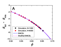
where $M_{k}=\overline{\sigma^{k}}$ ($k=1,2,3,\cdots$) are the $k$-th moments and $\Lambda=\sqrt{2\pi\beta\hbar^{2}/m}$ is the thermal de Broglie wavelength. Without loss of generality, we here set $\Lambda=1$. For continuous polydisperse systems one needs to pay special attention to the mixing entropy, $s_{\rm mix}$ Salacuse and Stell (1982); Frenkel (2014). We get back to this point in Sec. F.3. For now, we report $s_{\rm tot}-s_{\rm mix}$ for $N=1000$ and $8000$ in Fig. S4(A).

In order to validate the numerical thermodynamic integration, we also consider an analytical approximation of the equation of state (EOS). The polydisperse version of the Carnahan-Starling EOS, i.e., the so-called BMCSL EOS Boublík (1970); Mansoori et al. (1971),

$$Z_{\rm BMCSL}(\phi)=\frac{1}{1-\phi}+\frac{3M_{1}M_{2}}{M_{3}}\frac{\phi}{(1-\phi)^{2}}+\frac{M_{2}^{3}}{M_{3}^{2}}\frac{(3-\phi)\phi^{2}}{(1-\phi)^{3}},$$ (7)

is known to describe experiments and simulations of polydisperse hard-sphere systems rather well in the liquid regime. We also consider a modified version of $Z_{\rm BMCSL}$,

$$Z_{\rm modBMCSL}(\phi)=1+h(\phi)(Z_{\rm BMCSL}(\phi)-1),$$ (8)

where $h(\phi)=0.005-\tanh(14(\phi-0.79))$ Berthier et al. (2016c). Both EOSs trace our simulation data very well, as can be seen in Figs. S1 and S4(A). These EOSs can thus also be used to extrapolate the configurational entropy toward very high volume fraction (Sec. F.4).

Figure S4: (A) The total entropy, $s_{\rm tot}$, minus the mixing contribution, $s_{\rm mix}$, from simulations and from the (modified) BMCSL EOS. (B) The vibrational entropy, $s_{\rm vib}$, as a function of $\phi$ for several $\alpha_{\rm min}$. The solid straight line is fitted to the $N=1000$ results with $\alpha_{\rm min}=7.5\times 10^{0}$ in the high $\phi$ region.

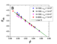
F.2 Vibrational entropy

The vibrational entropy, $s_{\rm vib}$, is obtained by Frenkel-Ladd (FL) thermodynamic integration Frenkel and Smit (2001); Angelani and Foffi (2007) by performing MC simulations of a constrained system with Hamiltonian

$$\beta H(\alpha)=\beta H(0)+\alpha\sum_{i=1}^{N}({\bf r}_{i}-{\bf r}_{0i})^{2},$$ (9)

for a template configuration, $\{{\bf r}_{0i}\}$, obtained from an equilibrium target system under $H(0)$. In short, the FL method integrates from a large $\alpha_{\rm max}\gg 1$, at which particles experience a nearly pure harmonic oscillator, down to a very weak $\alpha_{\rm min}\ll 1$, at which particles vibrate within cages. The vibrational entropy is then obtained by

$$s_{\rm vib} = \frac{3}{2}-\ln\Lambda^{3}-\frac{3}{2}\ln\left(\frac{\alpha_{\rm max}}{\pi}\right)+\int_{\alpha_{\rm min}}^{\alpha_{\rm max}}{\rm d}\alpha\delta r^{2}(\alpha)+\alpha_{\rm min}\delta r^{2}(\alpha_{\rm min}),$$ (10)

$$\delta r^{2}(\alpha) = \left[\left\langle\frac{1}{N}\sum_{i=1}^{N}({\bf r}_{i}-{\bf r}_{0i})^{2}\right\rangle_{\alpha}\right],$$ (11)

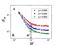
where $\langle(\cdots)\rangle_{\alpha}$ and $[(\cdots)]$ denote the thermal average with Hamiltonian $H(\alpha)$ and averaging over template configurations, $\{{\bf r}_{0i}\}$, respectively, and $\delta r^{2}$ in Eq. (11) is the mean-squared displacement shown in Fig. 2(A) of the main text.

Numerical integration of $\delta r^{2}$ is performed from $\alpha_{\rm max}$ to $\alpha_{\rm min}$. We set $\alpha_{\rm max}=7.5\times 10^{6}$, which is well into the harmonic-oscillator scaling regime [see Fig. 2(A) of the main text],

$$\delta r^{2}(\alpha_{\rm max})=\frac{3}{2\alpha_{\rm max}}.$$ (12)

The choice of $\alpha_{\rm min}$ is such that $\delta r^{2}$ of the constrained system is comparable to the mean-squared displacement of the target system without constraint. The last term in Eq. (10) corresponds to assuming a constant $\delta r^{2}$ for $\alpha\in[0,\alpha_{\rm min}]$ in the thermodynamic integration. In Fig. S4(B), we show $s_{\rm vib}$ for $N=1000$ and $8000$, with $\alpha_{\min}=1.5\times 10^{0}$, $7.5\times 10^{0}$, and $3.0\times 10^{1}$. At high volume fraction $\phi$, the results are insensitive to the choice of $\alpha_{\rm min}$, as expected. We can thus confidently set $\alpha_{\rm min}=7.5\times 10^{0}$. Also, we empirically observe a linear relation between $s_{\rm vib}$ and $\phi$, which allows us to linearly extrapolate the fit and thus the configurational entropy (see Sec. F.4).

F.3 Mixing entropy

The mixing entropy of the continuous polydisperse system formally diverges in the thermodynamic limit because each particle in the system then belongs to one of an infinite number of different components Salacuse and Stell (1982); Frenkel (2014). One, however, can subtract from this quantity a physically relevant contribution, which we call the effective mixing entropy, $s_{\rm mix}^{*}$. The main idea is that a continuous polydisperse system can be regarded as an effective $M^{*}$-component system (see Ref. Sollich (2001) and references therein). We then assume that the effective $M^{*}$-component system shares physical properties, in particular a same (free-)energy basin, with the original continuous polydisperse system. Here, a practical description of how to estimate $s_{\rm mix}^{*}$ from this scheme in our system is provided; a full explanation is provided in Ref. Ozawa and Berthier (2017).

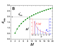
To estimate $M^{*}$, we first decompose the distribution $f(\sigma)$ into $M$ species, as shown in the inset of Fig. S5(B). We define $M$ species by dividing $f(\sigma)$ into equal intervals $\Delta\sigma=(\sigma_{\rm max}-\sigma_{\rm min})/M$, such that each species occupies the same fraction of the total volume, $A\rho\pi\Delta\sigma/6=C$, where $C$ is a constant. Note that $M$ is an integer and that $M\to\infty$ corresponds to the original continuous polydisperse system. We then perform a quench of the discretized system from the original configuration, and determine whether or not it remains in the same glassy basin as the original system by measuring the mean-squared displacement before and after the quench,

$$\Delta_{M}=\left[\frac{1}{N}\sum_{i=1}^{N}|{\bf r}_{Mi}^{\rm IS}-{\bf r}_{0i}|^{2}\right],$$ (13)

where $\{{\bf r}_{Mi}^{\rm IS}\}$ is the inherent structure configuration of a $M$-discretized system. If $M$ is large, the discretized system is almost identical with the original continuous polydisperse system and stays within the same basin, hence $\Delta_{M}\simeq\Delta_{M\to\infty}$. If $M$ is small, however, discretization destroys the glassy basin of the original system. The system thus structurally rearranges into a different glassy basin, and $\Delta_{M}\gg\Delta_{M\to\infty}$. This determination is done here by considering inherent structures, which for hard-sphere systems correspond to an out-of-equilibrium compression up to jamming Stillinger and Weber (1985). We determine $M^{*}$ as the crossover between these two limit cases.

More precisely, we follow the following algorithm.

1. Obtain an equilibrium configuration of the original continuous polydisperse system, $\{{\bf r}_{0i}\}$, for the initial configuration.

2. Discretize the diameters $\sigma$ of the original system into $M$ species, keeping $\phi$ fixed.

3. Quench the system to its inherent structure, $\{{\bf r}_{Mi}^{\rm IS}\}$, using the algorithm described in Refs. Xu et al. (2005); Desmond and Weeks (2009).

4. Repeat 1) - 3) for a range of $M$ and over different initial configurations.

5. Determine the crossover $M^{*}$ from $\Delta_{M}$ as a function of $M$.

In Fig. S5(A), we show how $\Delta_{M}$ evolves with $M$. At large $M$, $\Delta_{M}$ is flat and near $\Delta_{M\to\infty}$. The discretized system stays in its original basin. Upon decreasing $M$, however, $\Delta_{M}$ deviates from $\Delta_{M\to\infty}$, indicating that the discretized system escapes its basin. We estimate $M^{*}$ as an onset of this deviation by fitting the two linear lines from large and small $M$ regions. We find a weak $\phi$ dependence with $M^{*}\approx 9-10$ for all $\phi$ considered. We use linear fits to more precisely locate the crossover at $M^{*}=9.13$, see Fig. S5(A).

We map $M^{*}$ onto the effective mixing entropy $s_{\rm mix}^{*}$ by computing $s_{\rm mix}$ for different $M$,

$$s_{\rm mix}(M) = -\sum_{m=1}^{M}X_{m}\ln X_{m},$$ (14)

$$X_{m} = \int_{\sigma_{\rm min}+(m-1)\Delta\sigma}^{\sigma_{\rm min}+m\Delta\sigma}\mathrm{d}\sigma f(\sigma),$$ (15)

where $X_{m}$ is the concentration of species $m$. Fig. S5(B) shows the resulting $s_{\rm mix}(M)$. From the mapping indicated by the arrows, we obtain $s_{\rm mix}^{*}=1.98$. Note that $s_{\rm mix}^{*}$ in Fig. S5(B) varies relatively weakly with $M^{*}$ and so a more precise estimate of the value of $M^{*}$ is not needed for our purposes.

Figure S5: (A) Mean-squared displacement $\Delta_{M}$ between configurations before and after the quench. The crossover, $M^{*}$, is determined from the intersection of the two linear regimes at small and large $M$. (B) The mixing entropy $s_{\rm mix}$ as a function of $M$ from Eqs. (14) and (15). The dashed arrows map $M^{*}$ onto $s_{\rm mix}^{*}$. The inset shows the continuous polydispersity distribution, $f(\sigma)$, and the weights of delta functions for the discretized distribution with $M=5$, $\left\{X_{m}\right\}_{m=1,\ldots,5}$, as an example.

F.4 Configurational entropy

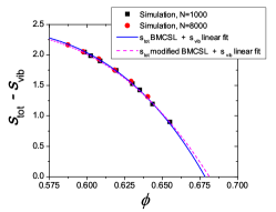
Using the above results, we obtain the configurational entropy from $s_{\rm tot}-s_{\rm vib}$ as a function of $\phi$. As can be seen in Fig. S6, no significant difference is observed between $N=1000$ and $8000$. We also find that the combination of $s_{\rm tot}$ from the (modified) BMCSL EOS in Fig. S4(A) and $s_{\rm vib}$ from the linear fit in Fig. S4(B) gives a reasonable extrapolation toward $s_{\rm tot}-s_{\rm vib}=0$, and thus an estimate for the Kauzmann transition, $\phi_{\rm K}\approx 0.68$ ($Z_{\rm K}\approx 45$). In Fig. 3 from the main text we use the curve extrapolated by the modified BMCSL EOS.

Figure S6: Configurational entropy $s_{\rm tot}-s_{\rm vib}$ as a function of volume fraction $\phi$, including the effective mixing entropy $s_{\rm mix}=s_{\rm mix}^{*}=1.98$. The solid (dashed) curve is a combination of $s_{\rm tot}$ from the (modified) BMCSL EOS and $s_{\rm vib}$ from the linear fit.

Appendix G Methods 2 and 3: The Franz-Parisi free energy

In this section we detail the Franz-Parisi construction Franz and Parisi (1997). We describe the order parameter of the glass transition, the umbrella sampling, as well as the parallel tempering and histogram reweighting techniques used to measure numerically the configurational entropy defined by Methods 2 and 3. Because the presentation closely follows earlier reports in which the Franz-Parisi free energy was determined numerically Berthier (2013); Berthier and Coslovich (2014); Berthier and Jack (2015), we only provide a brief summary of the computational methodology used.

G.1 Order parameter

The order parameter of the Franz-Parisi construction is the overlap $Q$ (or similarity) between two disordered configurations, defined as

$$Q=\frac{1}{N}\sum_{i,j}\theta(a-|{\bf r}_{1,i}-{\bf r}_{2,j}|),$$ (16)

where $\theta(x)$ is the Heaviside function, and ${\bf r}_{1,i}$ and ${\bf r}_{2,j}$ are the positions of particle $i$ and $j$ within configurations 1 and 2, respectively. By definition, $Q$ is large when the density fields in configurations 1 and 2 are very close, and $Q$ is close to zero when the density profiles are uncorrelated. The length, $a=0.23$, accounts for small-amplitude thermal vibrations, so that density profiles that only differ by local vibrations caused by thermal fluctuations have $Q$ close to unity.

G.2 Umbrella sampling

First, a reference configuration, $\{{\bf r}_{2}\}$, is chosen at random from the equilibrium states of the system at a fixed volume fraction. In order to access the probability distribution function of the overlap $Q_{12}$ between configurations $\{{\bf r}_{1}\}$ and $\{{\bf r}_{2}\}$, we conduct $n$ distinct simulations. In each simulation, $\ell=1,\cdots,n$, system 1 evolves according to the Hamiltonian

$$H_{\ell}=H(\{{\bf r}_{1}\})-\varepsilon Q_{12}+W_{\ell}(Q_{12}),$$ (17)

where $H(\{{\bf r}\})$ is the original hard-sphere Hamiltonian and $\varepsilon$ is the thermodynamic field conjugate to the overlap $Q_{12}$. The biasing potential $W_{\ell}(Q)$ is taken to have the form

$$W_{\ell}(Q)=k_{\ell}(Q-Q_{\ell})^{2},$$ (18)

with parameters $(k_{\ell},Q_{\ell})$ chosen to constrain the overlap $Q_{12}$ to explore values away from its average equilibrium value. We then perform local displacements and swap MC moves, which are accepted using a Metropolis acceptance rate given by the Hamiltonian (17).

Provided that the system is properly thermalized, our measurements yield the equilibrium probability distribution function of the overlap,

$$P_{\ell}(Q,\varepsilon,\phi)=\langle\delta(Q-Q_{12})\rangle_{\ell},$$ (19)

where $\langle\cdots\rangle_{\ell}$ denotes the thermal average with Hamiltonian $H_{\ell}$ in Eq. (17) at fixed reference configuration 2. Because we perform a quenched average to compute the overlap distribution, however, a second averaging, over the reference configuration 2, is needed to determine the Franz-Parisi free energy.

The idea behind the biasing potentials $W_{\ell}(Q)$ in Eqs. (17), and (18) is that the fluctuations of the overlap in each simulation can be tailored to explore a narrow region centered around $Q_{\ell}$. Each simulation thus explores but a small range of overlap values, and it becomes unnecessary to wait for very rare overlap fluctuations to take place. Umbrella sampling enables the efficient measure of the atypical overlap fluctuations needed to reconstruct the Franz-Parisi free energy.

G.3 Parallel tempering

While the umbrella sampling technique described above considerably accelerates the measurement of overlap fluctuations, we have observed that when $\phi$ is high, $N$ is large, and/or $Q_{\ell}$ is large, the particle dynamics still slows down considerably. It then becomes difficult to perform an accurate sampling of the overlap fluctuations imposed by the Hamiltonian (17).

To accurately sample the density regime explored in the present work, we have implemented parallel tempering MC moves Hukushima and Nemoto (1996). We conduct the $n$ simulations needed for the umbrella sampling at volume fraction $\phi$ in parallel, and propose MC exchange moves between neighboring simulations, as characterized by nearby sets of parameters, say $(k_{\ell},Q_{\ell})$ and $(k_{\ell+1},Q_{\ell+1})$. An exchange between simulations $\ell$ and $\ell+1$ is proposed with a low frequency (typically every $10^{3}$ MC sweeps) and they are accepted with a Metropolis acceptance rate given by the Hamiltonians $H_{\ell}$ and $H_{\ell+1}$, ensuring detailed balance.

Because each simulation now performs a random walk in the parameter space defined by $\{(k_{\ell},Q_{\ell}),\,\ell=1,\cdots,n\}$, the sampling of overlap fluctuations is greatly enhanced. For the method to be efficient, however, we need to adjust the biasing potentials $W_{\ell}(Q)$ such that the distributions $P_{\ell}(Q)$ of neighboring simulations overlap significantly. We have used up to $n=20$ to gather data. Thermalization was carefully checked by running long simulations (up to $10^{10}$ MC sweeps per simulation), in order to make sure that each state point was visited several times by all simulations via the replica exchange. This represents a significant numerical effort.

G.4 Histogram reweighting

Having obtained thermalized results from $n$ biased simulations run in parallel, we process the simulation outcome using multi-histogram reweighting methods to reconstruct the unbiased probability $P(Q)$ from the independently measured $P_{\ell}(Q)$,

$$P(Q,\varepsilon,\phi)=\frac{\sum_{\ell=1}^{n}P_{\ell}(Q,\varepsilon,\phi)}{\sum_{\ell=1}^{n}e^{-\beta W_{\ell}}/Z_{\ell}},$$ (20)

where $Z_{\ell}$ are defined self-consistently as

$$Z_{\ell}=\int_{0}^{1}{\rm d}Q^{\prime}\frac{\sum_{m=1}^{n}P_{j}(Q^{\prime},\varepsilon,\phi)}{\sum_{m=1}^{n}e^{\beta(W_{\ell}-W_{m})}/Z_{m}}.$$ (21)

Note that the actual value of $\varepsilon$ used in simulations plays no conceptual role because reweighting directly provides $P(Q,\varepsilon^{\prime},\phi)$ from $P(Q,\varepsilon,\phi)$ for distinct field values $\varepsilon$ and $\varepsilon^{\prime}$:

$$P(Q,\varepsilon^{\prime},\phi)=\frac{P(Q,\varepsilon,\phi)e^{-\beta Q(\varepsilon^{\prime}-\varepsilon)}}{\int_{0}^{1}{\rm d}Q^{\prime}P(Q^{\prime},\varepsilon,\phi)e^{-\beta Q^{\prime}(\varepsilon^{\prime}-\varepsilon)}}.$$ (22)

Two values of the field $\varepsilon$ are nonetheless particularly relevant to determining the configurational entropy, as described in the following two subsections.

G.5 Method 2

First, the Franz-Parisi free energy $V(Q)$ is obtained as

$$V(Q)=-\lim_{\varepsilon\to 0}\left[\frac{T}{N}\ln P(Q,\varepsilon,\phi)\right],$$ (23)

where $[\cdots]$ denotes averaging over the quenched reference configuration 2. We used 60 independent reference configurations for each value of the volume fraction. Because $V(Q)$ is only defined up to an additive constant, we arbitrarily adjust it, such that $V(Q_{\rm low})=0$, where $Q_{\rm low}\approx 0.05$ is defined as the location of the global minimum in $V(Q)$. This additive constant is irrelevant because only the free energy difference,

$$s_{\rm conf}=V(Q_{\rm high})-V(Q_{\rm low})\quad{\rm(Method\ 2)}$$ (24)

is needed to determine the configurational entropy. In this work, we set $Q_{\rm high}=0.8$ as motivated in the following subsection.

G.6 Method 3

Second, we obtain the critical field value $\varepsilon=\varepsilon^{\star}$ needed to induce a phase coexistence between low and high overlap states Franz and Parisi (1997); Berthier and Jack (2015). In practice, we use the strength of the reweighting method to finely explore a range of $\varepsilon$ values, and define $\varepsilon^{\star}$ as the field strength for which the overlap shows a value intermediate between $Q_{\rm low}$ and $Q_{\rm high}$, where the distribution $P(Q,\varepsilon^{\star},\phi)$ shows two peaks of equal amplitude, and where the variance of the overlap fluctuations (the susceptibility) is maximal. The position of the second peak of $P(Q,\varepsilon^{\star},\phi)$ at coexistence sets $Q_{\rm high}$. Because its volume fraction dependence is very weak, we fix it close to its average value and use $Q_{\rm high}=0.8$ for all $\phi$. Note that a secondary minimum cannot exist in the large system size limit of finite-dimensional simulations Berthier and Coslovich (2014), which is why we resort to the above definition of $Q_{\rm high}$.

The field $\varepsilon^{\star}$ has a simple graphical interpretation. It represents the amplitude of the field needed to ‘tilt’ the potential $V(Q)$ towards coexistence [see Fig. 2(B) of the main text]. Because the relation $V(Q_{\rm high})\approx\varepsilon^{\star}(Q_{\rm high}-Q_{\rm low})$, holds to a good approximation, $\varepsilon^{\star}$ provides an estimate of the free energy difference $V(Q_{\rm high})-V(Q_{\rm low})$. We can thus define the configurational entropy as

$$s_{\rm conf}=\varepsilon^{\star}(Q_{\rm high}-Q_{\rm low})\quad{\rm(Method\ 3)}.$$ (25)

Appendix H Method 4: The point-to-set correlation

H.1 Definition of cavity core overlap and point-to-set correlations

The similarity between two configurations, ${\bf X}=\left\{{\bf x}_{i}\right\}$ and ${\bf Y}=\left\{{\bf y}_{i}\right\}$, is characterized by using an overlap field, $q_{\bf X,Y}\left({\bf r}\right)$, computed as in Ref. Berthier et al. (2016b). For each particle ${\bf x}_{i}$, we find the nearest particle ${\bf y}_{i_{\rm nn}}$ and assign an overlap value $q_{{\bf X;Y}}\left({\bf x}_{i}\right)\equiv w\left(\big{|}{\bf x}_{i}-{\bf y}_{i_{\rm nn}}\big{|}\right)$, where

$$w(z)\equiv{\rm exp}\left[-\left(\frac{z}{b}\right)^{2}\right],$$ (26)

with $b=0.23$. This function defines overlap values $q_{\bf X;Y}\left({\bf x}_{i}\right)$ at scattered points $\left\{{\bf x}_{i}\right\}$. We then define a continuous function passing through these points, $q_{\bf X;Y}\left({\bf r}\right)$. Specifically, we first perform a Delaunay tessellation of space and, to a point ${\bf r}$ within a simplex spanned by four points $\left\{{\bf x}_{i}\right\}_{i=i_{1},i_{2},i_{3},i_{4}}$, associate a linearly interpolated value

$$q_{\bf X;Y}\left({\bf r}\right)=\sum_{i=i_{1},i_{2},i_{3},i_{4}}c_{i}q_{\bf X}\left({\bf x}_{i}\right),$$ (27)

where $\left\{c_{i}\right\}_{i=i_{1},i_{2},i_{3},i_{4}}$ satisfies ${\bf r}=\sum_{i=i_{1},i_{2},i_{3},i_{4}}c_{i}{\bf x}_{i}$ with the constraint $\sum_{i=i_{1},i_{2},i_{3},i_{4}}c_{i}=1$. We can similarly obtain $q_{\bf Y;X}\left({\bf r}\right)$, allowing us to define the overlap field

$$q_{\bf X,Y}\left({\bf r}\right)\equiv\frac{1}{2}\left\{q_{\bf X;Y}\left({\bf r}\right)+q_{\bf Y;X}\left({\bf r}\right)\right\}\,.$$ (28)

In order to capture the similarity between two configurations near the center of the cavity, we also define the cavity core overlap

$$q_{\rm c}\equiv\frac{3}{4\pi r_{\rm c}^{3}}\int_{|{\bf r^{\prime}}|<r_{\rm c}}{\rm d}{\bf r^{\prime}}\ q_{\bf X,Y}\left({\bf r^{\prime}}\right),$$ (29)

where $r_{\rm c}=0.576$ and ${\bf r^{\prime}}={\bf 0}$ is the cavity center. This integral is numerically evaluated by Monte Carlo integration using $10^{4}$ points.

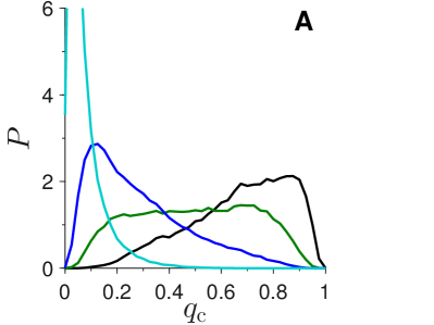
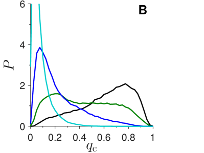
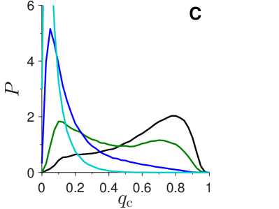
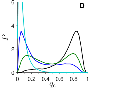
For each volume fraction $\phi$ and cavity radius $R$, the point-to-set correlation function, $Q_{\rm PTS}(R;\phi)$, is evaluated by disorder-averaging over $40$ cavity centers and, within each cavity, thermal-averaging over $s_{\rm{prod}}$ pairs of equilibrated configurations (see Tables 4-10) Berthier et al. (2016b). We extract the point-to-set correlation length through the compressed exponential fit,

$$Q_{\rm PTS}(R;\phi)=A\exp[-\left\{R/\xi_{\rm PTS}(\phi)\right\}^{\gamma}]+Q_{\rm PTS}^{\rm bulk}(\phi),$$ (30)

with the compressed exponent $\gamma=4$. Here the bulk value, $Q_{\rm PTS}^{\rm bulk}$, corresponds to the value at $R=\infty$ and is evaluated by taking $10^{5}$ pairs of independent configurations in bulk samples.

At the point-to-set length scale, we expect the probability distribution function of core overlaps to display broad fluctuations. Figure S7 bears out this expectation. In particular, as anticipated in Ref. Berthier et al. (2016b), we observe that the full disorder-averaged distribution becomes bimodal at high volume fractions, showing that we have indeed entered a deeply glassy regime that remains currently inaccessible for a standard binary Lennard-Jones liquid (see also Coslovich et al. (2017)).

Figure S7: Disorder-averaged probability distribution function of core overlap $P(q_{\rm c})$, at volume fractions $\phi=0.568$ (A), $0.597$ (B), $0.618$ (C), and $0.640$ (D) with varying radius $R=R_{1}$ (black), $R_{2}$ (green), $R_{3}$ (blue), and $R_{4}$ (cyan). We chose $(R_{1},R_{2},R_{3},R_{4})|_{\phi=0.568}=(1.38,1.73,2.07,3.11)$; $(R_{1},R_{2},R_{3},R_{4})|_{\phi=0.597}=(1.90,2.25,2.59,3.46)$; $(R_{1},R_{2},R_{3},R_{4})|_{\phi=0.618}=(2.25,2.59,3.11,4.15)$; and $(R_{1},R_{2},R_{3},R_{4})|_{\phi=0.640}=(2.77,3.46,3.80,5.18)$.

H.2 Parallel-tempering sampling with fuzzy-ensemble replicas

Denote positions of mobile particles inside the cavity $\mathbf{x}^{\rm M}_{i}$ with $i=1,\ldots,N_{\rm cav}$ and their associated diameters $\sigma^{\rm M}_{i}$. Similarly, denote positions and diameters of pinned particles outside the cavity $\mathbf{x}^{\rm P}_{j}$ and $\sigma^{\rm P}_{j}$, respectively. For cavity point-to-set measurements, one samples cavity configurations $\left\{\mathbf{x}^{\rm M}_{i}\right\}$ with probability

$$P\left(\left\{\mathbf{x}^{\rm M}_{i}\right\}\big{|}\left\{\sigma^{\rm M}_{i}\right\},\left\{\mathbf{x}^{\rm P}_{j}\right\},\left\{\sigma^{\rm P}_{j}\right\}\right)$$

$$\simeq {\rm exp}\left[-\beta U\left(\left\{\mathbf{x}^{\rm M}_{i}\right\},\left\{\sigma^{\rm M}_{i}\right\},\left\{\mathbf{x}^{\rm P}_{j}\right\},\left\{\sigma^{\rm P}_{j}\right\}\right)\right],$$

where $\simeq$ denotes equality up to a normalization constant and a hard wall constraint $\big{|}{\bf x}^{\rm M}_{i}\big{|}<R$ at the edge of the cavity of size $R$ is imposed. Note that for the standard hard-sphere potential, $U$, this expression does not depend on the inverse temperature $\beta\in\left(0,\infty\right)$. Properly sampling from this weight can be computationally demanding, because the equilibration time grows rapidly both as the cavity size decreases and as the volume fraction increases (see Fig. S8 and Sec. H.4). In these systems, phase space can actually become fully disconnected, which makes proper sampling impossible through (semi-)local Monte Carlo moves.

We here overcome this difficulty through a parallel-tempering algorithm Frenkel and Smit (2001); Fukunishi et al. (2002). The simplest scheme, analogous to that employed in Ref. Berthier et al. (2016b) for a thermal binary Lennard-Jones liquid, would be to couple the above ensemble with replicas governed by a probability

$$P_{\lambda}\left(\left\{\mathbf{x}^{\rm M}_{i}\right\}\big{|}\left\{\sigma^{\rm M}_{i}\right\},\left\{\mathbf{x}^{\rm P}_{j}\right\},\left\{\sigma^{\rm P}_{j}\right\}\right)$$

$$\simeq {\rm exp}\left[-\beta U\left(\left\{\mathbf{x}^{\rm M}_{i}\right\},\left\{\lambda\sigma^{\rm M}_{i}\right\},\left\{\mathbf{x}^{\rm P}_{j}\right\},\left\{\sigma^{\rm P}_{j}\right\}\right)\right]\,,$$

where the diameter of the particles inside the cavity is uniformly shrunk by $\lambda$. This approach, however, is highly inefficient for hard interactions. Replica-swap attempts are indeed very likely to be rejected, because even small $\lambda$ increments can result in hard overlaps. More precisely, in order to have appreciable replica-swapping acceptance rates, the spacing between consecutive $\lambda$’s must scale as $O(1/N_{\rm cav})$, and thus $O(N_{\rm cav})$ replicas are needed, as opposed to $O(\sqrt{N_{\rm cav}})$ for thermal systems Frenkel and Smit (2001).

We therefore introduce a fuzzy ensemble governed by probability weights controlled by two parameters, $\alpha$ and $\hat{\lambda}$,

$$P_{\alpha,\hat{\lambda}}\left(\left\{\mathbf{x}^{\rm M}_{i}\right\},\lambda\ \big{|}\left\{\sigma^{\rm M}_{i}\right\},\left\{\mathbf{x}^{\rm P}_{j}\right\},\left\{\sigma^{\rm P}_{j}\right\}\right)$$

$$\simeq {\rm exp}\left\{-\frac{\alpha^{2}N_{\rm cav}}{2}\left(\lambda-\hat{\lambda}\right)^{2}\right\}\,$$

$$\times{\rm exp}\left[-\beta U\left(\left\{\mathbf{x}^{\rm M}_{i}\right\},\left\{\lambda\sigma^{\rm M}_{i}\right\},\left\{\mathbf{x}^{\rm P}_{j}\right\},\left\{\sigma^{\rm P}_{j}\right\}\right)\right]\,,$$

hence the shrinking factor $\lambda$ is allowed to fluctuate. With this modification, a $O(\sqrt{N_{\rm cav}})$ scaling for the number of replicas needed is recovered. One caveat is that one of the replicas must obey the original sharp distribution defined in Eq. (H.2)–formally corresponding to the limit $\alpha\rightarrow\infty$ with $\hat{\lambda}=1$–and the aforementioned challenge imposed by hard interactions still persists for that case. This problem is here surmounted by using a large number of replica-swap attempts near the original replica–$O(1000N_{\rm cav})$ more frequent than others–as detailed in Sec. H.3.2.

H.3 Details of Monte Carlo moves

This section details the implementation of the Monte Carlo scheme for the cavity simulations.

H.3.1 Basic moves within a replica

Within each replica, we perform Monte Carlo moves consisting of local displacements, particle identity swaps, and, for fuzzy ensembles, diameter fluctuations.

• Local displacements consist of: (i) randomly choosing a particle $i$ from the $N_{\rm cav}$ mobile particles within the cavity; (ii) displacing particle $i$ by $\Delta{\bf x}=l\hat{\bf{n}}$ with uniform $l\in[0,0.1]$ and uniform $\hat{\bf{n}}$ on the unit sphere $S^{2}$; and (iii) accepting displacement only if no hard overlaps are created. Note that an additional hard spherical wall at the edge of the cavity guarantees that mobile particles cannot leave the cavity–a rare instance, even at the lowest volume fraction studied.

• Particle identity swaps consist of: (i) choosing two distinct particles $i$ and $j$ within a cavity; and (ii) swapping their diameters if it results in no hard overlaps. (For the highest volume fraction $\phi=0.640$ with the cavity size $R\geq 3.11$, in order to accelerate runs, we attempt these moves only for pairs with diameter difference $\lambda|\sigma_{i}-\sigma_{j}|<0.086$.)

• Diameter fluctuations consist of: (i) uniformly drawing a shift $\Delta\lambda\in\left[-\frac{0.2}{\alpha\sqrt{N_{\rm cav}}},+\frac{0.2}{\alpha\sqrt{N_{\rm cav}}}\right]$, and (ii) accepting the shift with probability $p={\rm min}\{p_{\Lambda},1\}$, where

  $$p_{\Lambda}={\rm exp}\left[-\frac{\alpha^{2}N_{\rm cav}}{2}\left\{\left(\lambda+\Delta\lambda-\hat{\lambda}\right)^{2}-\left(\lambda-\hat{\lambda}\right)^{2}\right\}\right]\,,$$ (34)

  if no hard overlaps are created.

One MC sweep consists of $N_{\rm cav}$ MC trial moves of the above kinds for each replica. For large cavities with $R>\xi_{\rm PTS}+1$, each MC sweep consists of $N_{\rm cav}$ MC trial moves with $70\%$ ($80\%$) local displacements and $30\%$ ($20\%$) particles identity swaps (parenthesis are for $\phi=0.640$) alone. For small cavities, however, proper sampling requires replica exchange and diameter fluctuations (see Fig. S8).

H.3.2 Parallel tempering

For parallel tempering, we label replicas $a=1,\ldots,n$, where $a=1$ corresponds to the original ensemble with $\hat{\lambda}_{1}=1$ and $\alpha_{1}=\infty$. For the other replicas, we choose $\alpha_{a\geq 2}=20$, and $\{\hat{\lambda}_{a}\}$ are tuned to enable appreciable replica-swap rate (see below). For $a\geq 3$, each MC sweep consists of $N_{\rm cav}$ MC trial moves with $60\%$ ($70\%$) local displacements, $30\%$ ($20\%$) particles identity swaps, and $10\%$ diameter fluctuations (parenthesis are for $\phi=0.640$ with $R\geq 3.11$). For $a=1$ and $a=2$, a different scheme is employed. The two cavities are run as a pair with a large number of replica-swap attempts. Each MC sweep consists of $4N_{\rm cav}$ attempts, $50\%$ replica-swap between $\left\{\mathbf{x}^{\rm M}_{i}\right\}_{1}$ and $\left\{\mathbf{x}^{\rm M}_{i}\right\}_{2}$ –accepted only when swapping $\lambda_{1}=1$ and $\lambda_{2}$ does not result in hard overlaps–, $15\%$ ($17.5\%$) local displacements respectively for $a=1$ and $a=2$, $7.5\%$ ($5\%$) particles identity swaps respectively for $a=1$ and $a=2$, and $5\%$ diameter fluctuations for $a=2$.

For each $a\geq 2$, a replica-identity swap between $\left(\left\{\mathbf{x}^{\rm M}_{i}\right\}_{a},\lambda_{a}\right)$ and $\left(\left\{\mathbf{x}^{\rm M}_{i}\right\}_{a+1},\lambda_{a+1}\right)$ is attempted every $1000$ MC sweeps on average, with acceptance probability $p={\rm min}\{p_{\rm RS},1\}$, where

$$p_{\rm RS}={\rm exp}\left\{-\alpha^{2}N_{\rm cav}\left(\hat{\lambda}_{a+1}-\hat{\lambda}_{a}\right)\left(\lambda_{a+1}-\lambda_{a}\right)\right\}\,.$$ (35)

The replica parameters, $\{\hat{\lambda}_{a}\}_{a\geq 2}$, are tuned to ensure sufficient replica-swap rates. In order to achieve this sampling, we first define the average of the fluctuating $\lambda$

$$\langle\lambda\rangle_{a}=\int{\rm d}\lambda{\rm d}\mathbf{x}^{\rm M}_{i}\ \lambda\ P_{\alpha_{a},\hat{\lambda}_{a}}\left(\left\{\mathbf{x}^{\rm M}_{i}\right\},\lambda\ \big{|}\left\{\sigma^{\rm M}_{i}\right\},\left\{\mathbf{x}^{\rm P}_{j}\right\},\left\{\sigma^{\rm P}_{j}\right\}\right)\,,$$ (36)

For the replica $a=2$, we ensure that $\langle\lambda\rangle_{2}=1+O\left(\sqrt{\langle\lambda^{2}\rangle_{2}-\langle\lambda\rangle_{2}^{2}}\right)$, which typically requires $\hat{\lambda}_{2}>1$, because of the relatively high system pressure. Replicas are then added one by one, with $\hat{\lambda}_{2}>\hat{\lambda}_{3}>\ldots>\hat{\lambda}_{n}$, each time targeting a replica-swap acceptance rate of $\sim 20\%$. This process is stopped upon reaching $\hat{\lambda}_{n}$, such that $\langle\lambda\rangle_{n}<\lambda_{\rm dec}$ (see Tables 4-10). Although this linear approach does not attain a globally uniform replica-swap acceptance rate (see Katzgraber et al. (2006); Vogel and Perez (2015) for more systematic approaches), the resulting scheme suffices to ensure equilibration and convergence, as defined in the next subsection.

The concerted use of replica exchange, fuzzy ensembles, and specialized sampling scheme around the original ensemble provides a sufficient number of independent cavity configurations from the desired ensemble defined in Eq. (H.2).

H.3.3 Convergence criterion

The quality of equilibration within each cavity is evaluated by monitoring the convergence of two initialization schemes Cavagna et al. (2012); Berthier et al. (2016b): (i) from the original configuration, and (ii) from a randomized configuration prepared by first running $10^{6}$ MC sweeps with shrunk cavity particles at $(\hat{\lambda},\alpha)=(0.5,20)$ and then slowly regrowing particles back to $\lambda=1$. We then record configurations every $t_{\rm rec}$ MC sweeps (see Tables 4-10), and monitor the core overlap between new configurations and the original configuration, $q_{\rm c}^{\rm on}\left(t\right)$, as a function of the number of MC sweeps, $t$. The first $s_{\rm eq}$ configurations are discarded, and the average overlap for the following $s_{\rm prod}$ configurations,

$$\langle q_{\rm c}^{\rm on}\rangle\equiv\frac{1}{s_{\rm prod}}\sum_{s=s_{\rm eq}+1}^{s_{\rm eq}+s_{\rm prod}}q_{\rm c}^{\rm on}\left(t_{\rm rec}s\right)\,,$$ (37)

is computed. Convergence is deemed achieved when the results of both approaches lie within $\pm 0.1$ of each other for each cavity. This criterion also allows us to estimate the convergence time for a given value of $R$ and $\phi$. Replica parameters as well as $s_{\rm eq}$ and $s_{\rm prod}$ (see Tables 4-10) are chosen, such that at least $95\%$ out of $40$ cavities pass this convergence test, except for the most challenging data point, $(\phi,R)=(0.640,3.80)$, where a $92.5\%$ rate was tolerated. Because the difference between the two approaches is not systematic, however, averaging over $40$ cavities results in a rather close agreement between the two schemes, i.e., they converge within $\pm 0.01$.

H.4 Swap is not enough

Figure S8: Characteristic convergence time (in unit of MC sweeps) multiplied by the number of replicas with (blue-square) and without (red-circle) replica exchange, as a function of cavity size $R$. Note that the result without replica exchange at $R=2.42$ is an underestimate, because particle swaps alone did not allow the results to converge even after $5\cdot 10^{9}$ MC sweeps. Convergence is also not achieved for $R=1.73$.

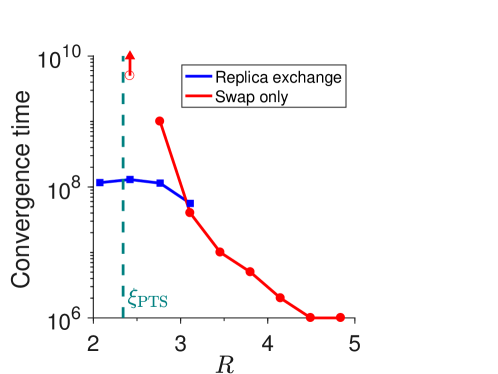
It has been suggested that particle identity swaps by themselves suffice to thermalize cavities, especially small ones with $R<\xi_{\rm PTS}$ Biroli et al. (2008); Cavagna et al. (2012). We here test this hypothesis for our polydisperse system, for which particle swaps are extremely effective at sampling bulk configurations. Figure S8 contrasts the computational time needed to equilibrate cavity configurations at $\phi=0.608$, with and without parallel tempering. Without replica exchange, the equilibration time rapidly grows as the cavity size decreases, which is in line with the suggestion that confinement enhances the breaking of ergodicity Berthier et al. (2016b). We observe that when $R$ approaches the point-to-set length from above, however, the convergence time becomes too long to be measured. Tests performed with even smaller $R$ values confirm that trend. Convergence is never achieved for cavities of the order of the point-to-set length or smaller. By contrast, using replica exchange with swap dynamics keeps convergence time within computational reach even for small cavities.

This result seems to contrast with the findings of Ref. Cavagna et al. (2012) that the dynamics actually speeds up inside small cavities. We have no explanation for this discrepancy as we never observed such speed-up in any of our simulations, but we note that the timescale studied in Ref. Cavagna et al. (2012) is different from the one shown in Fig. S8. Specifically, whereas we report a convergence time for the overlap inside the cavity, Cavagna et al. study the time decay of the overlap-fluctuation auto-correlation function in equilibrium. We have not tried to systematically measure this latter auto-correlation because it is already very clear that, according to the former convergence criterion, we cannot properly thermalize small cavities in simulations that use identity swaps alone. Therefore, we would not access an equilibrium correlation timescale but a nonequilibrium one. In addition, no quantitative analysis of the convergence time is provided in Refs. Biroli et al. (2008); Cavagna et al. (2012), which makes a direct comparison with our results impossible.

We conclude that one must generally employ a parallel-tempering scheme, as developed in Ref. Berthier et al. (2016b), in order to properly sample small cavities and measure point-to-set correlations.

$R$		$1.38$	$1.73$	$2.07$	$2.42$	$2.77$	$3.11$	$3.46$	$3.80$	$4.15$
$n_{\rm ave}$		10	8	7	7	6	1	1	1	1
$\lambda_{\rm dec}$		0.850	0.920	0.960	0.970	0.980	NA	NA	NA	NA
$t_{\rm rec}$		4000	4000	4000	4000	4000	1000	400	200	200
$s_{\rm eq}$		500	500	500	500	500	500	500	500	500
$s_{\rm prod}$		2000	2000	2000	2000	2000	2000	2000	2000	2000

Table 4: Cavity PTS measurement parameters $\phi=0.568$. Runs without parallel tempering have $n_{\rm ave}=1$.

$R$		$1.73$	$2.07$	$2.42$	$2.77$	$3.11$	$3.46$	$3.80$	$4.15$	$4.49$
$n_{\rm ave}$		10	10	10	8	7	1	1	1	1
$\lambda_{\rm dec}$		0.900	0.930	0.950	0.970	0.980	NA	NA	NA	NA
$t_{\rm rec}$		$2\cdot 10^{4}$	$2\cdot 10^{4}$	$2\cdot 10^{4}$	$10^{4}$	4000	2000	1000	400	400
$s_{\rm eq}$		500	500	500	500	500	500	500	500	500
$s_{\rm prod}$		2000	2000	2000	2000	2000	2000	2000	2000	2000

Table 5: Cavity PTS measurement parameters $\phi=0.587$. Runs without parallel tempering have $n_{\rm ave}=1$.

$R$		$1.90$	$2.25$	$2.59$	$2.94$	$3.11$	$3.46$	$3.80$	$4.15$	$4.49$
$n_{\rm ave}$		12	13	12	11	9	1	1	1	1
$\lambda_{\rm dec}$		0.900	0.920	0.940	0.960	0.970	NA	NA	NA	NA
$t_{\rm rec}$		$2\cdot 10^{4}$	$2\cdot 10^{4}$	$2\cdot 10^{4}$	$10^{4}$	$10^{4}$	$10^{4}$	4000	2000	1000
$s_{\rm eq}$		500	500	500	500	500	500	500	500	500
$s_{\rm prod}$		2000	2000	2000	2000	2000	2000	2000	2000	2000

Table 6: Cavity PTS measurement parameters $\phi=0.597$. Runs without parallel tempering have $n_{\rm ave}=1$.

$R$		$2.07$	$2.42$	$2.77$	$3.11$	$3.46$	$3.80$	$4.15$	$4.49$	$4.84$
$n_{\rm ave}$		13	14	12	12	1	1	1	1	1
$\lambda_{\rm dec}$		0.910	0.920	0.950	0.960	NA	NA	NA	NA	NA
$t_{\rm rec}$		$2\cdot 10^{4}$	$2\cdot 10^{4}$	$2\cdot 10^{4}$	$10^{4}$	$2\cdot 10^{4}$	$10^{4}$	4000	2000	2000
$s_{\rm eq}$		500	500	500	500	500	500	500	500	500
$s_{\rm prod}$		2000	2000	2000	2000	2000	2000	2000	2000	2000

Table 7: Cavity PTS measurement parameters $\phi=0.608$. Runs without parallel tempering have $n_{\rm ave}=1$.

$R$		$2.25$	$2.42$	$2.59$	$3.11$	$3.80$	$4.15$	$4.49$	$4.84$
$n_{\rm ave}$		15	16	18	17	1	1	1	1
$\lambda_{\rm dec}$		0.900	0.910	0.910	0.940	NA	NA	NA	NA
$t_{\rm rec}$		$10^{4}$	$10^{4}$	$10^{4}$	$10^{4}$	$5\cdot 10^{4}$	$3\cdot 10^{4}$	$10^{4}$	5000
$s_{\rm eq}$		2000	2000	2000	1000	500	500	500	500
$s_{\rm prod}$		8000	8000	8000	4000	2000	2000	2000	2000

Table 8: Cavity PTS measurement parameters $\phi=0.618$. Runs without parallel tempering have $n_{\rm ave}=1$.

$R$		$2.77$	$2.94$	$3.11$	$3.46$	$3.80$	$4.49$	$4.84$
$n_{\rm ave}$		17	19	18	17	16	1	1
$\lambda_{\rm dec}$		0.930	0.930	0.940	0.955	0.965	NA	NA
$t_{\rm rec}$		$10^{4}$	$10^{4}$	$10^{4}$	$10^{4}$	$10^{4}$	$10^{5}$	$4\cdot 10^{4}$
$s_{\rm eq}$		1500	3000	4000	6000	8000	500	500
$s_{\rm prod}$		6000	12000	16000	9000	12000	2000	2000

Table 9: Cavity PTS measurement parameters $\phi=0.629$. Runs without parallel tempering have $n_{\rm ave}=1$.

$R$		$2.77$	$3.11$	$3.46$	$3.63$	$3.80$	$4.84$	$5.18$
$n_{\rm ave}$		21	21	22	23	22	1	1
$\lambda_{\rm dec}$		0.910	0.930	0.940	0.940	0.950	NA	NA
$t_{\rm rec}$		$10^{4}$	$10^{4}$	$10^{4}$	$10^{4}$	$10^{4}$	$2\times 10^{5}$	$10^{5}$
$s_{\rm eq}$		2000	6000	8000	12000	12000	1000	1000
$s_{\rm prod}$		8000	9000	12000	18000	18000	4000	4000

Table 10: Cavity PTS measurement parameters $\phi=0.640$. Runs without parallel tempering have $n_{\rm ave}=1$.

Appendix I Method 1 for soft spheres

We compute the configurational entropy of a continuous polydisperse soft sphere system by the standard definition,

$$s_{\rm conf}=s_{\rm tot}-s_{\rm vib},$$ (38)

where $s_{\rm tot}$ and $s_{\rm vib}$ are the total and vibrational entropies Sciortino et al. (1999); Sastry (2001). The mixing entropy is also treated by the strategy used in Ref. Ozawa and Berthier (2017); we compute $s_{\rm tot}$ and $s_{\rm vib}$ as if the system were monodisperse, and then add the effective mixing entropy $s_{\rm mix}^{*}$ independently determined in simulations Ozawa and Berthier (2017).

I.1 Model

We use a continuous size polydispersity, where the particle diameter $\sigma$ of each particle is randomly drawn from the following particle size distribution: $f(\sigma)=A\sigma^{-3}$, for $\sigma\in[\sigma_{\rm min},\sigma_{\rm max}]$, where $A$ is a normalization constant. We define the size polydispersity as $\Delta=\sqrt{\overline{\sigma^{2}}-\overline{\sigma}^{2}}/\overline{\sigma}$, where $\overline{\cdots}=\int\mathrm{d}\sigma f(\sigma)(\cdots)$. We use $\Delta=0.23$, choosing $\sigma_{\rm min}/\sigma_{\rm max}=0.4492$, and set $\overline{\sigma}$ as the unit length. We simulate systems composed of $N$ particles in a cubic cell of volume $V$ with periodic boundary conditions in three dimensions, $d=3$. We use the following pairwise potential for the soft sphere model,

$$v_{ij}(r) = v_{0}\left(\frac{\sigma_{ij}}{r}\right)^{n}+c_{0}+c_{1}\left(\frac{r}{\sigma_{ij}}\right)^{2}+c_{2}\left(\frac{r}{\sigma_{ij}}\right)^{4},$$ (39)

$$\sigma_{ij} = \frac{(\sigma_{i}+\sigma_{j})}{2}(1-\epsilon|\sigma_{i}-\sigma_{j}|),$$ (40)

where $v_{0}$ is the unit of energy, and $\epsilon$ quantifies the degree of non-additivity of the particle diameters. Non-additivity conveniently prevents crystallization and thus enhances the glass-forming ability of the model. The constants, $c_{0}$, $c_{1}$ and $c_{2}$, are chosen so that the first and second derivatives of $v_{ij}(r)$ vanish at the interaction cut-off $r_{\rm cut}=1.25\sigma_{ij}$. We employ the non-additive soft sphere model with parameters $n=12$ and $\epsilon=0.2$, and set the number density to $\rho=N/V=1.0$ for $N=1500$ particles.

Equilibrium configurations are produced by swap MC simulations after high temperature configurations are instantaneously quenched to the target temperature. Equilibration is ensured by the fact that particles lose memory of their initial positions and dynamical observables do not present aging. The absence of crystalline nuclei is also verified. We additionally perform standard MC simulations to obtain relaxation times down to the mode coupling crossover temperature $T_{\rm c}$. Following the procedure described in the Materials and methods section of the main text, we carry out three kinds of fits on these dynamical data. First we employ a power-law fit to extrapolate $T_{\rm c}=0.104$. We then perform a VFT fit with $\delta=1$ and a parabolic fit to estimate the glass-ceiling temperature $T_{\rm g}=0.0720-0.0817$.

I.2 Total entropy

Figure S9: (A) Plot of $\beta^{3/4}e(\beta)$ vs. $\beta^{1/4}$ to extract the fit parameters, $A$, $B$, and $C$, in Eq. (46). The solid line is the resulting fitting curve. The vertical arrow indicates the position of $\beta_{0}$. (B) $s_{\rm tot}-s_{\rm mix}$ as a function of $T$. The dashed curve is the Rosenfeld-Tarazona expression, $s_{\rm tot}-s_{\rm mix}+3\ln\Lambda\propto T^{-2/5}$, which is well confirmed by our data.

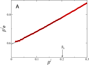
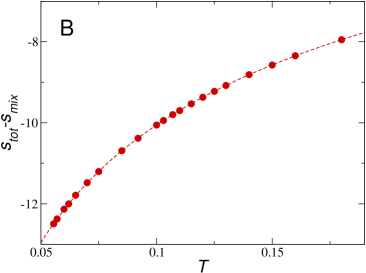
We perform the thermodynamic integration over the inverse temperature $\beta^{\prime}$ from the ideal gas limit $\beta^{\prime}\to 0$ to the target temperature $\beta$,

$$s_{\rm tot}(\beta)=\frac{5}{2}-\ln\rho-3\ln\Lambda+\beta e(\beta)-\int_{0}^{\beta}\mathrm{d}\beta^{\prime}e(\beta^{\prime})+s_{\rm mix},$$ (41)

where $e(\beta)$ is the potential energy of the system and for this system we set $m=1$ and $\hbar=1$ such that the thermal de Broglie wavelength $\Lambda=\sqrt{2\pi\beta}$.

Special care is needed to compute the integral in Eq. (41) because the potential energy $e(\beta)$ diverges in the high temperature limit Coluzzi et al. (2000); Ozawa et al. (2015). To accurately calculate the integral, we thus decompose the integration range into a very high temperature regime, $\beta^{\prime}\in[0,\beta_{0}]$, and an intermediate regime, $\beta^{\prime}\in(\beta_{0},\beta]$, with $\beta_{0}$ the boundary between the two regimes. Therefore, the integral in Eq. (41) can be decomposed as

$$I = \int_{0}^{\beta}\mathrm{d}\beta^{\prime}e(\beta^{\prime})=\int_{0}^{\beta_{0}}\mathrm{d}\beta^{\prime}e(\beta^{\prime})+\int_{\beta_{0}}^{\beta}\mathrm{d}\beta^{\prime}e(\beta^{\prime})$$ (42)

$$= I_{\rm F}+I_{\rm N},$$ (43)

where $I_{\rm F}$ and $I_{\rm N}$ are integrals over the very high and the intermediate temperature regimes, respectively. We set $\beta_{0}=1.68\times 10^{-3}$ in this work. The integral $I_{\rm N}$ can be performed by usual numerical integration. To obtain $I_{\rm F}$ we fit the potential energy data to a polynomial function, then analytically integrate the function, which enables us to avoid the numerical integration of the diverging $e(\beta\to 0)$ Coluzzi et al. (2000); Ozawa et al. (2015). In a three-dimensional system of particles interacting via $v(r)\propto r^{-12}$, the high temperature expansion of the potential energy reads:

$$e(\beta)=A\beta^{-3/4}+B\beta^{-1/2}+C\beta^{-1/4}+O\left(\beta^{0}\right)\,,$$ (44)

where $A$, $B$, and $C$ are constants. Using Eqs. (43) and (44), we get

$$I_{\rm F}=4A\beta_{0}^{1/4}+2B\beta_{0}^{1/2}+(4/3)C\beta_{0}^{3/4}+O\left(\beta_{0}\right).$$ (45)

Therefore, we can compute $I_{\rm F}$ from the fitting parameters, $A$, $B$, and $C$.

In order to obtain $A$, $B$, and $C$ by fitting, we rewrite Eq. (44) as

$$\beta^{3/4}e(\beta)=A+B\left(\beta^{1/4}\right)+C\left(\beta^{1/4}\right)^{2}+O\left(\beta^{3/4}\right),$$ (46)

and use a quadratic fit as shown in Fig. S9(A).

Figure S9(B) shows the results for $s_{\rm tot}-s_{\rm mix}$. The dashed line corresponds to the Rosenfeld-Tarazona (RT) expression Rosenfeld and Tarazona (1998) $e(T)\propto T^{3/5}$ or $s_{\rm tot}+3\ln\Lambda\propto T^{-2/5}$, which allows us to extrapolate to lower temperatures. Figure S9(B) confirms that the RT expression works very well over our simulation range.

I.3 Vibrational entropy

Figure S10: (A) The harmonic vibrational entropy $s_{\rm harm}$ and anharmonic correction $s_{\rm anh}$. Dashed curves are obtained by quadratic fit to $(1/N)\sum_{a=1}^{3N}\{1-\ln(\omega_{a})\}$. (B) The anharmonic contribution of the potential energy $e_{\rm anh}(T)$. The solid line is obtained by fitting over a range $T\in[0.0555,0.125]$

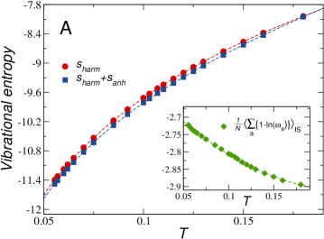
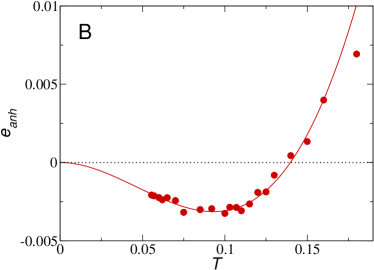
We compute the vibrational entropy $s_{\rm vib}$ by

$$s_{\rm vib}=s_{\rm harm}+s_{\rm anh},$$ (47)

where $s_{\rm harm}$ and $s_{\rm anh}$ are the harmonic vibrational entropy and the anharmonic correction, respectively Sciortino (2005). We compute $s_{\rm harm}$ Sciortino et al. (1999); Sastry (2001) using

$$s_{\rm harm}(\beta)=\frac{1}{N}\left\langle\sum_{a=1}^{3N}\{1-\ln(\beta\hbar\omega_{a})\}\right\rangle_{\rm IS},$$ (48)

where $\langle\cdots\rangle_{\rm IS}$ denotes an average over the inherent structure obtained by the conjugate gradient method, and $\omega_{a}=\sqrt{\lambda_{a}/m}$, and $\lambda_{a}$ is the eigenvalue of the Hessian. In Fig. S10(A), we show $s_{\rm harm}$ as a function of $T$. In order to extrapolate $s_{\rm harm}$ to lower temperatures, we follow the common scheme of fitting $(1/N)\langle\sum_{a=1}^{3N}\{1-\ln(\omega_{a})\}\rangle_{\rm IS}$ to a second-degree polynomial in $T$ Sciortino et al. (1999); Flenner and Szamel (2006).

We also evaluate the anharmonic contribution $s_{\rm anh}$ Sciortino (2005) to the potential energy,

$$e_{\rm anh}(T)=e(T)-e_{\rm IS}(T)-\frac{3}{2}T,$$ (49)

where $e_{\rm IS}$ is the inherent structure energy. The last term is the energy of the harmonic vibration. Using $e_{\rm anh}(T)$, $s_{\rm anh}(T)$ is given by

$$s_{\rm anh}(T)=\int_{0}^{T}\mathrm{d}T^{\prime}\frac{1}{T^{\prime}}\frac{\partial e_{\rm anh}(T^{\prime})}{\partial T^{\prime}}.$$ (50)

when assuming that there is no anharmonic contribution at $T=0$, i.e., $s_{\rm anh}(T=0)=0$. Expanding $e_{\rm anh}(T)$ around zero temperature then gives

$$e_{\rm anh}(T)=\sum_{k=2}a_{k}T^{k},$$ (51)

where $a_{k}$ is a $T$ independent coefficient. We also assume the linear term in Eq. (51) is zero, $a_{1}=0$, which means that the anharmonic contribution to the specific heat vanishes at $T=0$. Substituting Eq. (51) into Eq. (50), we obtain

$$s_{\rm anh}(T)=\sum_{k=2}\frac{k}{k-1}a_{k}T^{k-1}.$$ (52)

In Fig. S10(B), we show a fit of $e_{\rm anh}$ using $a_{2}$ and $a_{3}$, and in Fig. S10(A) we show $s_{\rm harm}+s_{\rm anh}$. We find that the anharmonic contribution is small, $|s_{\rm anh}|<0.08$, over our range of interest, and thus that the details of the above procedure have little influence on the final estimate of $s_{\rm vib}$.

I.4 Mixing entropy

Figure S11: The effective mixing entropy $s_{\rm mix}^{*}$. The dashed line is an empirical linear fit.

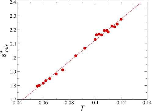
We include the effective mixing entropy $s_{\rm mix}^{*}$ obtained by an independent set of simulations in Ref. Ozawa and Berthier (2017). In contrast to the hard sphere system, $s_{\rm mix}^{*}$ of the soft sphere system has a weakly linear temperature dependence on the control parameter as shown in Fig. S11. A linear fit, $s_{\rm mix}^{*}=b_{0}+b_{1}T$, gives $b_{0}=1.3601$ and $b_{1}=7.6565$.

I.5 Configurational entropy

Figure S12: The configurational entropy of soft spheres, $s_{\rm conf}=s_{\rm tot}-s_{\rm vib}$. The glass ceiling is indicated in the blue region and the dashed curve is an extrapolation based on separately fitting the individual terms. The mode-coupling crossover temperature $T_{\rm c}$ is denoted by a vertical arrow.

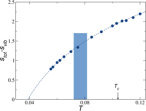
The resulting configurational entropy $s_{\rm conf}$ is shown in Fig. S12. The data demonstrates that $s_{\rm conf}$ decreases further below the experimental glass transition, and does not show any sign of a crossover, bending, or saturation. Also, combining the extrapolations for $s_{\rm tot}$, $s_{\rm harm}$, $s_{\rm anh}$, and $s_{\rm mix}^{*}$, we extrapolate $s_{\rm conf}$ down to zero, and estimate the Kauzmann transition to be around $T_{\rm K}\simeq 0.04$. We conclude from this analysis that the results reported in the main text for hard spheres are not specific to this interaction potential. Our methods thus apply equally well to models of supercooled liquids characterized by continuous pair potentials.

References

- Kauzmann (1948) W. Kauzmann, Chem. Rev. 43, 219 (1948).
- Kirkpatrick and Thirumalai (1987) T. R. Kirkpatrick and D. Thirumalai, Phys. Rev. B 36, 5388 (1987).
- Kirkpatrick and Wolynes (1987) T. R. Kirkpatrick and P. G. Wolynes, Phys. Rev. B 36, 8552 (1987).
- Charbonneau et al. (2014a) P. Charbonneau, J. Kurchan, G. Parisi, P. Urbani, and F. Zamponi, Nat. Commun. 5, 3725 (2014a).
- Berthier and Biroli (2011) L. Berthier and G. Biroli, Rev. Mod. Phys. 83, 587 (2011).
- Kirkpatrick et al. (1989) T. R. Kirkpatrick, D. Thirumalai, and P. G. Wolynes, Phys. Rev. A 40, 1045 (1989).
- Stillinger (1988) F. H. Stillinger, J. Chem. Phys. 88, 7818 (1988).
- Garrahan and Chandler (2003) J. P. Garrahan and D. Chandler, Proc. Natl. Acad. Sci. U.S.A. 100, 9710 (2003).
- Dyre (2006) J. Dyre, Rev. Mod. Phys. 78, 953 (2006).
- Wyart (2010) M. Wyart, Phys. Rev. Lett. 104, 095901 (2010).
- Rabochiy et al. (2013a) P. Rabochiy, P. G. Wolynes, and V. Lubchenko, J. Phys. Chem. B 117, 15204 (2013a).
- Sciortino et al. (1999) F. Sciortino, W. Kob, and P. Tartaglia, Phys. Rev. Lett. 83, 3214 (1999).
- Berthier and Coslovich (2014) L. Berthier and D. Coslovich, Proc. Natl. Acad. Sci. U.S.A. 111, 11668 (2014).
- Petzold et al. (2013) N. Petzold, B. Schmidtke, R. Kahlau, D. Bock, R. Meier, B. Micko, D. Kruk, and E. Rössler, J. Chem. Phys. 138, 12A510 (2013).
- Brambilla et al. (2009) G. Brambilla, D. El Masri, M. Pierno, L. Berthier, L. Cipelletti, G. Petekidis, and A. B. Schofield, Phys. Rev. Lett. 102, 085703 (2009).
- Barrat et al. (1990) J.-L. Barrat, J.-N. Roux, and J.-P. Hansen, Chem. Phys. 149, 197 (1990).
- Kob and Andersen (1994) W. Kob and H. C. Andersen, Phys. Rev. Lett. 73, 1376 (1994).
- Martinez and Angell (2001) L.-M. Martinez and C. Angell, Nature 410, 663 (2001).
- Grigera and Parisi (2001) T. S. Grigera and G. Parisi, Phys. Rev. E 63, 045102 (2001).
- Berthier et al. (2016a) L. Berthier, D. Coslovich, A. Ninarello, and M. Ozawa, Phys. Rev. Lett. 116, 238002 (2016a).
- Ninarello et al. (2017a) A. Ninarello, L. Berthier, and D. Coslovich, Phys. Rev. X 7, 021039 (2017a).
- Angelani and Foffi (2007) L. Angelani and G. Foffi, J. Phys. Cond. Matter 19, 256207 (2007).
- Berthier et al. (2016b) L. Berthier, P. Charbonneau, and S. Yaida, J. Chem. Phys. 144, 024501 (2016b).
- Pusey and Van Megen (1986) P. Pusey and W. Van Megen, Nature 320, 340 (1986).
- Berthier and Witten (2009) L. Berthier and T. A. Witten, Phys. Rev. E 80, 021502 (2009).
- Stickel et al. (1995) F. Stickel, E. W. Fischer, and R. Richert, J. Chem. Phys. 102, 6251 (1995).
- Frenkel and Ladd (1984) D. Frenkel and A. J. Ladd, J. Chem. Phys. 81, 3188 (1984).
- Frenkel (2014) D. Frenkel, Mol. Phys. 112, 2325 (2014).
- Ozawa and Berthier (2017) M. Ozawa and L. Berthier, J. Chem. Phys. 146, 014502 (2017).
- Stillinger and Weber (1985) F. H. Stillinger and T. A. Weber, J. Chem. Phys. 83, 4767 (1985).
- Biroli and Monasson (2000) G. Biroli and R. Monasson, Europhys. Lett. 50, 155 (2000).
- Franz and Parisi (1997) S. Franz and G. Parisi, Phys. Rev. Lett. 79, 2486 (1997).
- Adam and Gibbs (1965) G. Adam and J. H. Gibbs, J. Chem. Phys. 43, 139 (1965).
- Bouchaud and Biroli (2004) J.-P. Bouchaud and G. Biroli, J. Chem. Phys. 121, 7347 (2004).
- Biroli et al. (2008) G. Biroli, J.-P. Bouchaud, A. Cavagna, T. S. Grigera, and P. Verrocchio, Nat. Phys. 4, 771 (2008).
- Lubchenko (2015) V. Lubchenko, Adv. Phys. 64, 283 (2015).
- Albert et al. (2016) S. Albert, T. Bauer, M. Michl, G. Biroli, J.-P. Bouchaud, A. Loidl, P. Lunkenheimer, R. Tourbot, C. Wiertel-Gasquet, and F. Ladieu, Science 352, 1308 (2016).
- Rabochiy et al. (2013b) P. Rabochiy, P. G. Wolynes, and V. Lubchenko, J. Phys. Chem. B 117, 15204 (2013b).
- Berthier et al. (2005) L. Berthier, G. Biroli, J.-P. Bouchaud, L. Cipelletti, D. E. Masri, D. L’Hote, F. Ladieu, and M. Pierno, Science 310, 1797 (2005).
- Charbonneau and Tarjus (2013) P. Charbonneau and G. Tarjus, Phys. Rev. E 87, 042305 (2013).
- Allen and Tildesley (1989) M. P. Allen and D. J. Tildesley, Computer simulation of liquids (Oxford University Press, 1989).
- Santos et al. (2005) A. Santos, S. B. Yuste, and M. L. de Haro, J. Chem. Phys. 123, 234512 (2005).
- Gazzillo and Pastore (1989) D. Gazzillo and G. Pastore, Chem. Phys. Lett. 159, 388 (1989).
- Sindzingre et al. (1989) P. Sindzingre, C. Massobrio, G. Ciccotti, and D. Frenkel, Chem. Phys. 129, 213 (1989).
- Santen and Krauth (2001) L. Santen and W. Krauth, arXiv preprint cond-mat/0107459 (2001).
- Pronk and Frenkel (2004) S. Pronk and D. Frenkel, Phys. Rev. E 69, 066123 (2004).
- Frenkel and Smit (2001) D. Frenkel and B. Smit, Understanding Molecular Simulation (Academic Press, New York, ed. 2., 2001).
- Brumer and Reichman (2004) Y. Brumer and D. R. Reichman, J. Phys. Chem. B 108, 6832 (2004).
- Gutiérrez et al. (2015) R. Gutiérrez, S. Karmakar, Y. G. Pollack, and I. Procaccia, Europhys. Lett. 111, 56009 (2015).
- Sastry et al. (1998) S. Sastry, P. G. Debenedetti, and F. H. Stillinger, Nature 393, 554 (1998).
- Charbonneau et al. (2014b) P. Charbonneau, Y. Jin, G. Parisi, and F. Zamponi, Proc. Natl. Acad. Sci. U.S.A. 111, 15025 (2014b).
- Boublík (1970) T. Boublík, J. Chem. Phys. 53, 471 (1970).
- Mansoori et al. (1971) G. A. Mansoori, N. F. Carnahan, K. E. Starling, and T. W. Leland Jr, J. Chem. Phys. 54, 1523 (1971).
- Berthier et al. (2016c) L. Berthier, P. Charbonneau, Y. Jin, G. Parisi, B. Seoane, and F. Zamponi, Proc. Natl. Acad. Sci. U.S.A. 113, 8397 (2016c).
- Vasisht et al. (2011) V. V. Vasisht, S. Saw, and S. Sastry, Nat. Phys. 7, 549 (2011).
- Shiba et al. (2012) H. Shiba, T. Kawasaki, and A. Onuki, Phys. Rev. E 86, 041504 (2012).
- Rycroft (2009) C. Rycroft, (2009).
- Ninarello et al. (2017b) A. Ninarello, L. Berthier, and D. Coslovich, Phys. Rev. X 7, 021039 (2017b).
- Elmatad et al. (2009) Y. S. Elmatad, D. Chandler, and J. P. Garrahan, J. Phys. Chem. B 113, 5563 (2009).
- Isobe et al. (2016) M. Isobe, A. S. Keys, D. Chandler, and J. P. Garrahan, Phys. Rev. Lett. 117, 145701 (2016).
- Richert and Angell (1998) R. Richert and C. Angell, J. Chem. Phys. 108, 9016 (1998).
- Sastry (2001) S. Sastry, Nature 409, 164 (2001).
- Salacuse and Stell (1982) J. Salacuse and G. Stell, J. Chem. Phys. 77, 3714 (1982).
- Sollich (2001) P. Sollich, J. Phys. Cond. Matter 14, R79 (2001).
- Xu et al. (2005) N. Xu, J. Blawzdziewicz, and C. S. O’Hern, Phys. Rev. E 71, 061306 (2005).
- Desmond and Weeks (2009) K. W. Desmond and E. R. Weeks, Phys. Rev. E 80, 051305 (2009).
- Berthier (2013) L. Berthier, Phys. Rev. E 88, 022313 (2013).
- Berthier and Jack (2015) L. Berthier and R. L. Jack, Phys. Rev. Lett. 114, 205701 (2015).
- Hukushima and Nemoto (1996) K. Hukushima and K. Nemoto, J. Phys. Soc. Jpn 65, 1604 (1996).
- Coslovich et al. (2017) D. Coslovich, L. Berthier, and M. Ozawa, SciPost Physics 3, 027 (2017).
- Fukunishi et al. (2002) H. Fukunishi, O. Watanabe, and S. Takada, J. Chem. Phys. 116, 9058 (2002).
- Katzgraber et al. (2006) H. G. Katzgraber, S. Trebst, D. A. Huse, and M. Troyer, J. Stat. Mech. 2006, P03018 (2006).
- Vogel and Perez (2015) T. Vogel and D. Perez, Phys. Rev. Lett. 115, 190602 (2015).
- Cavagna et al. (2012) A. Cavagna, T. S. Grigera, and P. Verrocchio, J. Chem. Phys. 136, 204502 (2012).
- Coluzzi et al. (2000) B. Coluzzi, G. Parisi, and P. Verrocchio, J. Chem. Phys. 112, 2933 (2000).
- Ozawa et al. (2015) M. Ozawa, W. Kob, A. Ikeda, and K. Miyazaki, Proc. Natl. Acad. Sci. U.S.A. 112, 6914 (2015).
- Rosenfeld and Tarazona (1998) Y. Rosenfeld and P. Tarazona, Mol. Phys. 95, 141 (1998).
- Sciortino (2005) F. Sciortino, J. Stat. Mech. 2005, P05015 (2005).
- Flenner and Szamel (2006) E. Flenner and G. Szamel, Phys. Rev. E 73, 061505 (2006).