Modeling and replicating statistical topology, and evidence for CMB non-homogeneity

Abstract

Under the banner of ‘Big Data’, the detection and classification of structure in extremely large, high dimensional, data sets, is, one of the central statistical challenges of our times. Among the most intriguing approaches to this challenge is ‘TDA’, or ‘Topological Data Analysis’, one of the primary aims of which is providing non-metric, but topologically informative, pre-analyses of data sets which make later, more quantitative analyses feasible. While TDA rests on strong mathematical foundations from Topology, in applications it has faced challenges due to an inability to handle issues of statistical reliability and robustness and, most importantly, in an inability to make scientific claims with verifiable levels of statistical confidence. We propose a methodology for the parametric representation, estimation, and replication of persistence diagrams, the main diagnostic tool of TDA. The power of the methodology lies in the fact that even if only one persistence diagram is available for analysis – the typical case for big data applications – replications can be generated to allow for conventional statistical hypothesis testing. The methodology is conceptually simple and computationally practical, and provides a broadly effective statistical procedure for persistence diagram TDA analysis. We demonstrate the basic ideas on a toy example, and the power of the approach in a novel and revealing analysis of CMB non-homogeneity.

AMS 2010 Subject Classification. Primary: 60G55, 62H12, 62H15.
Secondary: 62G05, 85A35.

Keywords. Persistence diagram, Hamiltonian, MCMC, Replicating statistical topology, CMB isotropy

1 Introduction

As a consequence of the current explosion in size, complexity, and dimensionality of data sets, there has been a growing need for the development of powerful but concise summary statistics and visualisation methods that facilitate understanding and decision making. A singularly novel approach, which has been particularly promising in areas as widespread as biology and medicine [33, 16, 27], neurophysiology, [18], cosmology [44, 38], and materials science [28], has been via the application of the powerful, and rather abstract, concepts of Algebraic Topology to develop what generally now falls under the label of ‘Topological Data Analysis’, or TDA. While approaching complex data from a topological viewpoint is not entirely new – it underlies Tukey’s ‘Exploratory Data Analysis’ of the 1960’s [46] and the more recent approach by Friston and coworkers to brain imaging data [30] – TDA differs from all its forebears in its sophisticated exploitation of recent developments in Computational Topology. In particular, much of TDA has become almost synonymous with an analysis based on some version of persistent homology [19, 20, 21], represented visually as barcodes, persistence diagrams, or related representations [13, 14, 25, 26, 48].

With relatively few exceptions, notably [17, 23, 41, 6, 10, 42], TDA has not employed statistical methodology as part of its approach, and, as a consequence, has typically been unable to associate clearly defined levels of statistical significance to its discoveries. While there may be a variety of reasons for this, one of the main obstacles to doing so is that the mathematical challenges involved in computing the statistical distributions of topological quantifiers have so far proven to be intractable. This is despite the fact that the measure-theoretic issues involved in defining probability spaces for objects related to persistent homology have indeed been solved; e.g. [32, 47].

One approach adopted by [17, 23, 41] and others to circumvent these difficulties has been to reduce persistence diagrams to a single test statistic, often related to bottleneck norms, and then to adopt standard statistical resampling methods to analyse this statistic. If multiple diagrams are available, then the resampling can be done on them. However, since TDA is typically used in areas of very large data sets, the availability of replicates is rare, and consequently this approach is impracticable in most applications. An alternative approach is to (sub)sample points from the persistence diagram, and compute statistics on the subsamples. The problem with this approach, however, is that the true random object here is the full persistence diagram, and it thus it is often unclear what is the precise meaning of the statistics produced this way.

We introduce a new approach, based on generating a sequence of persistence diagrams which has similar statistical properties to those of the one generated by the data. While novel, the ideas underlying the method are not difficult, and follow a number of clearly defined stages. Firstly, a parametric model is adopted that is sufficiently flexible to model an extremely wide class of persistence diagrams. The model we use is a class of Gibbs distributions, since these have a long history of success in modelling point sets, ([2] and its bibliography) and, in the final analysis, this is what a persistence diagram is. Having estimated parameters, we then exploit the fact that Gibbs distributions lend themselves to simulation by Markov chain Monte Carlo (MCMC) methods, and we exploit MCMC to produce a simulated sequence of diagrams. Since the underlying raison d’être of this approach is that persistence diagrams provide an excellent summary of topology, and statistics computed off the diagrams themselves furnish even more succinct summaries, we call this procedure Replicating Statistical Topology, or RST, and its introduction and the descriptions of its implementation are the main contributions of the paper. We believe that these ideas will provide a significant contribution towards putting TDA on a more solid statistical footing. To support this we shall treat one toy example, showing that the technique works as predicted, and then study the fascinating and important topic of non-homogeneities in the CMB (Cosmic Microwave Background) radiation using an RST approach.

2 TDA and persistence diagrams

As homology is an algebraic method for describing topological features of shapes and functions, so persistent homology is an extension of this method for both enriching these descriptions and for describing how topology undergoes changes. We shall use it to describe the upper-level sets of real-valued functions $f$ defined over a space ${\mathcal{X}}$; viz. sets of the form $A_{u}=\{x\in{\mathcal{X}}:\,f(x)\geq u\}$. In basic homology, the topology of each $A_{u}$ is often summarized by its Betti numbers, $\beta_{k}$, $k=0,\dots\text{dim}({\mathcal{X}})$. The first of these, $\beta_{0}$, counts the number of connected components in $A_{u}$, and, roughly speaking, the remaining $\beta_{k}$ count the number of $(k+1)$-dimensional ‘holes’ in $A_{u}$. Persistent homology goes further, and keeps track of how the homology, including the Betti numbers, changes as a function of the level $u$, giving a richer, more dynamic view of topology.

Today persistent homology is undeniably the most popular tool in the burgeoning area of TDA, one of the main reasons for which is the fact that it is easily visualised via barcode diagrams. Each bar in such a diagram is an interval that starts (is ‘born’ at) a level $b$, at which a new aspect of the homology of $A_{u}$ appears, and ends (‘dies’ at) a level $d$, as this aspect disappears. A mathematically equivalent, but visually distinct representation, of barcodes is as persistence diagrams, henceforth PDs, of the points $(b,d)$. We shall assume that the reader has some familiarity with these concepts, but look at an instructive, and easy, example in Fig. 1, needed later.

Figure 1: A random sample from two circles, 500 points from the larger circle and 300 from the smaller one, along with a kernel density estimate and the persistence diagram for its upper level sets. The black circles are the $H_{0}$ persistence points, while the red triangles are the $H_{1}$ points.

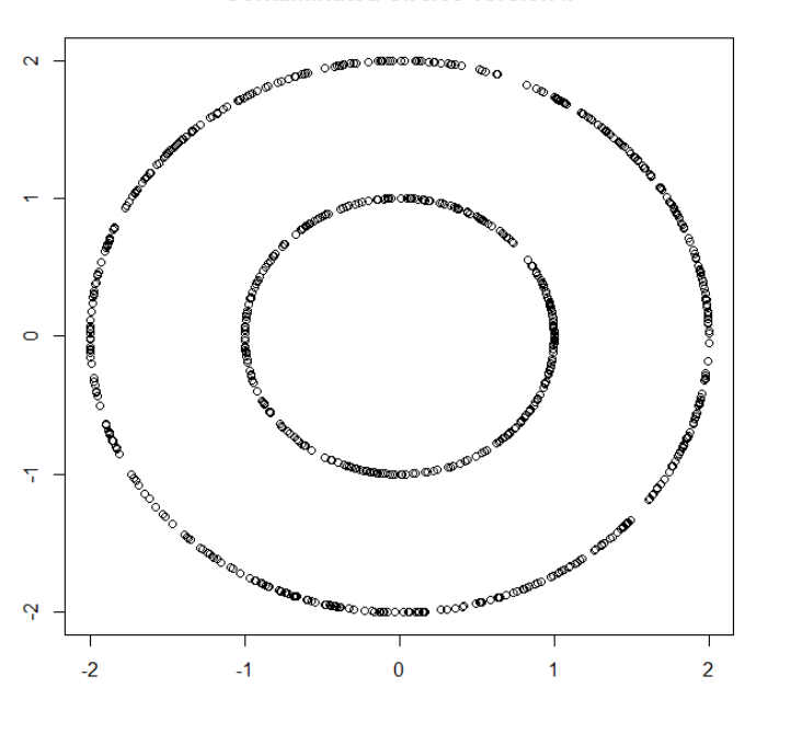
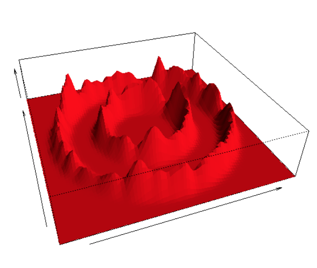
At the left, we see a sample ${\tilde{x}}_{N}=\{x_{1},\dots,x_{N}\}$ of $N=800$ points from two circles, of diameters 4 and 2. A random sample of 500 points were chosen at random from the larger circle, and 300 from the smaller one. To its right, we see the corresponding kernel density estimate, defined by

$$\hat{f}_{N}(p)\ =\ \frac{1}{N}\sum_{i=1}^{N}\frac{1}{2\pi\delta^{2}}e^{{-\|p-x_{i}\|^{2}}/{2\delta^{2}}},$$ (1)

where $\delta>0$ is a bandwidth parameter, the precise value of which is not important for now.

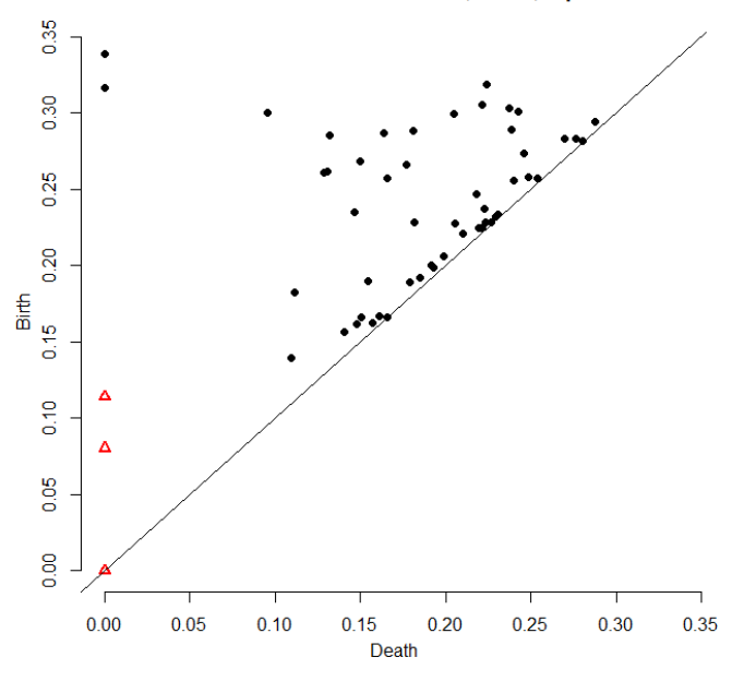
At the far right we have the corresponding persistence diagram of the upper level set filtration of $\hat{f}_{N}$, with the black circles indicating $H_{0}$ (zero-th homology) persistence and the red triangles corresponding to $H_{1}$, in both cases trying to capture the underlying homology of the two circles. As described above, each point in the diagram is a ‘birth-death’ pair $(b,d)$. The accepted paradigm of TDA is that points in the PD ‘far away’ from the diagonal $b=d$ are meaningful, while points close to the diagonal, which represent short lived topological phenomena, are not. Thus, since we know that the upper level sets of $\hat{f}_{N}$ are characterized by having two main components, each of which contains a single 1-cycle (hole) we expect to see two black circles and two red triangles somewhat isolated from the other points in the diagram. This is in fact the case.

While the PD in Fig.  1 performs as expected, and it is easy to identify the points that, a priori, we knew had to be there, there are many other points in the diagrams, and were we not in the situation of knowing ahead of time which points were ‘really’ significant, it would not have been clear how to discount the additional points. We shall see later how to do this, but first must describe the general approach.

3 Gibbs measures for persistence diagrams

Given a finite collection ${\tilde{X}}_{N}=\{X_{1},\dots,X_{N}\}$ of continuous random variables, with joint probability density $\varphi_{\Theta}({\tilde{x}}_{N})$, dependent on a multi-dimensional parameter $\Theta$, we say that $\varphi_{\Theta}$ is a Gibbs distribution if it is written in the form

$$\varphi_{\Theta}({\tilde{x}}_{N})=\frac{1}{Z_{\Theta}}\exp(-H_{\Theta}({\tilde{x}}_{N})),$$ (2)

where the ‘Hamiltonian’ $H_{\Theta}:\,\mathbb{R}^{N}\to\mathbb{R}$ describes the ‘energy’ of configurations ${\tilde{x}}_{N}$. The normalisation $Z_{\Theta}$, actually a function of $\Theta$, is known as the partition function, and is infamously hard to evaluate. All this is standard fare [24]. What is new is that we shall use Gibbs distributions to provide a model for PDs that look like those in Fig. 1. (There is another important family of PDs that arise from the construction of simplicial complexes over point sets, and these, at least for their $H_{0}$ diagrams, have all points with birth times identically zero. These are much easier to analyze, since they are effectively one dimensional, and we shall treat them in a separate publication.)

As in all applications of Gibbs distributions, success depends on an appropriate choice for the energy function. Here is a way to do it for ${\tilde{x}}_{N}$ a set of $N$ points in a subset ${\mathcal{X}}$ of $\mathbb{R}^{2}$. Firstly, for $x\in{\mathcal{X}}$ and, for $k,\delta>0$ let ${\mathcal{N}}_{\delta,k}(x)$ be the collection of the $k$ nearest neighbours of $x$ in ${\tilde{x}}_{N}$, assuming that all are of distance no greater than $\delta$ from $x$. If $k$ such points do not exist, then we take ${\mathcal{N}}_{\delta,k}(x)=\emptyset$.

Assign a weight, or total length to each such cluster, given by the sum of distances to its reference point, viz.

$$\mathcal{L}_{\delta,k}(x)\equiv\mathcal{L}_{\delta,k}(x\,|\,{\mathcal{N}}_{\delta,k}(x))=\sum_{y\in{\mathcal{N}}_{\delta,k}(x)}\|x-y\|.$$

The weight, or total length, of all $(k+1,\delta)$-clusters is then

$$\mathcal{L}_{\delta,k}\equiv\mathcal{L}_{\delta,k}({\tilde{x}}_{N})=\sum_{x\in{\tilde{X}}_{N}}\mathcal{L}_{\delta,k}(x).$$

Now, for $x\in{\mathcal{X}}$ write $x=(x^{(1)},x^{(2)})$, and

$$\sigma_{H}^{2}=\sum_{x\in{\tilde{x}}_{N}}\big{(}x^{(1)}-\bar{x}^{(1)}\big{)}^{2},\ \ \ \sigma_{V}^{2}=\sum_{x\in{\tilde{x}}_{N}}\big{(}x^{(2)}\big{)}^{2},$$

where $\bar{x}^{(1)}=N^{-1}\sum_{i=1}^{N}x_{i}^{(1)}$.

Thinking now, for reasons to become clear soon, of ${\mathcal{X}}=\mathbb{R}\times\mathbb{R}_{+}$, we define a Hamiltonian, at effective interaction distance $\delta$, up to cluster size $K\geq 0$, and with interaction parameter $\Theta=(\theta_{H},\theta_{V},\theta_{1},\dots,\theta_{K})$, as

$$H_{\delta,\Theta}^{K}({\tilde{x}}_{N})=\theta_{H}\sigma^{2}_{H}+\theta_{V}\sigma^{2}_{V}+\sum_{k=1}^{K}\theta_{k}\mathcal{L}_{\delta,k}({\tilde{x}}_{N}).$$ (3)

The parameters here all have a very clear meaning. The horizontal spread of the points in ${\tilde{x}}_{N}$ is controlled by $\sigma^{2}_{H}$, the vertical spread by $\sigma^{2}_{V}$, and each $\theta_{k}$ controls the probability of clusters of size $k+1$, with $\theta_{k}<0$ favouring such clusters, and $\theta_{k}>0$ lowering their probabilities.

Now, given a PD $\widetilde{B}=\{(b_{i},d_{i})\}_{i=1}^{N}$, define a new set of $N$ points ${\tilde{x}}_{N}=\{x_{i}\}_{i=1}^{N}$, with $x^{(1)}_{i}=b_{i}$ and $x^{(2)}_{i}=d_{i}-b_{i}$. This (invertible) transformation has the effect of moving the points in Fig. 1 downwards, so that the diagonal line projects onto the horizontal axis, but still leaves a visually informative diagram, which we shall call the projected PD, or PPD. The statistical model we take for PPDs is a Gibbs distribution (2) with Hamiltonian (3).

While this may seem a rather arbitrary form for the distribution of a PPD, there are two facts justifying it. The first is the trivial observation that any multivariate distribution can be written in the form (2), simply by taking $H_{\Theta}\equiv-\ln(\varphi_{\Theta})$ and $Z_{\Theta}=1$. The second is that, having done this, we would like to take $H$ from a rich enough family of functions to come close to spanning all ‘reasonable’ functions on PPDs. However, we know from [1] that the ring of algebraic functions on the space of PPDs is spanned by monomials of the form $(x^{(1)}_{1}-x^{(2)}_{1})^{m_{1}}(x^{(2)})^{n_{1}}\cdots(x^{(1)}_{l}-x^{(2)}_{l})^{m_{l}}(x^{(2)}_{l})^{n_{l}}$, for which $n_{i}>0$ implies $m_{i}>0$, and functions of the form (3) form a rich subset of these monomials. Furthermore, ‘cluster expansions’ of this form have been successfully employed in Statistical Mechanics for the best part of a century as a basic approximation tool in the study of Gibbs distributions.

The determination of $\delta$ depends on the number of the points $N$ on the persistence diagram, and on the spread of the points. In practice, theoretical results (cf. the reviews [29, 7]) suggest taking $\delta$ of the form

$$\delta=\frac{\delta^{*}}{N^{\alpha_{k,d}}}\max\left(\max|x^{(1)}_{i}-x^{(1)}_{j}|,\ \max|x^{(2)}_{i}-x^{(2)}_{j}|\right),$$ (4)

where $\alpha_{0,d}=1/d$, $\alpha_{k,d}={k/(k+1)d}$, for $k\geq 1$, $d$ is the dimension of the data underlying the PD, and $\delta^{*}$ is a data independent tuning parameter. The terms inside the brackets in (4) scale for the order of magnitude of the data, which is unimportant topologically. (For cases for which $d$ is unknown, setting $d=2$ seems to work in practice, merely leading to larger than usual values of $\delta^{*}$, as does ignoring the fine structure of $\alpha_{k,d}$ and taking it to be $1/\sqrt{N}$, as a global default.)

3.1 Pseudolikelihood

Given $H_{\Theta}$ as a parametric model, we now turn to the estimation problem. Unfortunately, estimation of the parameters by a method such as direct maximum likelihood is precluded by the fact that we neither have an analytic form for $Z_{\Theta}$, nor is there any way to compute it numerically in any reasonable time frame.

The standard way around this problem, which we adopt, is the pseudolikelihood approach [5, 15]. This originated in the context of point cloud data with spatial dependence, which is, essentially, a description of a PD. In particular, it exploits the inherent spatial Markovianess of a Gibbs distribution to replace the overall probability of, in our case, a random PPD ${\tilde{X}}_{N}$ by the pseudolikelihood

$$L^{K}_{\delta,\Theta}({\tilde{x}}_{N})\stackrel{{\scriptstyle\Delta}}{{=}}\prod_{x\in{\tilde{x}}_{N}}f_{\Theta}\left(x\big{|}N_{\delta,K}(x)\right),$$ (5)

where the conditional, local, densities $f_{\Theta}\left(x\big{|}N_{\delta,K}(x)\right)$ are given by

$$\frac{\exp\left(-H^{K}_{\delta,\Theta}\left(x\big{|}N_{\delta,K}(x)\right)\right)}{\int_{\mathbb{R}}\int_{\mathbb{R}_{+}}\exp\left(-H^{K}_{\delta,\Theta}\left(z\big{|}N_{\delta,K}(x)\right)\right)\,dz^{(1)}dz^{(2)},}$$ (6)

and the conditional, Hamiltonians $H^{K}_{\delta,\Theta}\left(x\big{|}N_{\delta,K}(x)\right)$ by

$$\theta_{H}\left[x^{(1)}-\bar{x}^{(1)}\right]^{2}+\theta_{V}(x^{(2)})^{2}+\sum_{k=1}^{K}\theta_{k}{\mathcal{L}}_{\delta,k}\left(x\big{|}N_{\delta,K}(x)\right).$$

3.2 Model specification and parameter estimation

While it might be expected that PPDs originating from different areas might require quite different models, we have found, in all the examples that we tried, that taking $K=2$ in (3) – so that the largest cluster size was 3 – was both efficient and sufficient. If a lower $K$ was appropriate, then the estimation procedure described above estimated the higher order parameters $\theta_{k}$ as close to zero. In this case, using standard, automated statistical procedures such as AIC, BIC, etc. (cf. [12]) we often deleted the corresponding clusters from the Hamiltonian. Overall, we found the procedure not to be sensitive to either these small parameters or the specific procedure adopted for deleting them. After considerable experimentation, we found that working with all parameters appearing when $K=2$, regardless of their absolute value, was the easiest thing to do. We also found that taking $K>2$ did little to improve the simulation procedure, and typically led to manifestations of overfitting.

4 RST and MCMC

We refer the reader to [40, 9] for technical background to this section, in which we describe a standard Metropolis-Hastings MCMC approach to replicating PDs.

Given a pseudolikelihood as in the previous section (with known or estimated parameters), generating simulated replications of the associated point set via MCMC is not hard, but first we need some definitions.

Firstly, given a ${\tilde{x}}_{N}$, take $q(\cdot|{\tilde{x}}_{N})$ to be the folded Gaussian density on $\mathbb{R}^{2}$ with mean vector and covariance matrix identical to the empirical mean and covariance of the points in ${\tilde{x}}_{N}$. Next, for two points $x,x^{*}\in{\mathcal{X}}$ define an ‘acceptance probability’, according to which we will replace $x\in{\tilde{x}}_{N}$ by $x^{*}$, thus giving the updated PPD ${\tilde{x}}_{N}^{*}$, as

$$\rho\left(x,x^{*}\right)=\min\left\{1,\frac{f_{\Theta}\left(x^{*}|N_{\delta,K}(x)\right)\cdot q(x|{\tilde{x}}^{*}_{N})}{f_{\Theta}\left(x|N_{\delta,K}(x)\right)\cdot q(x^{*}|{\tilde{x}}_{N})}\right\}.$$

(Note that integration in the denominator of $f_{\Theta}$ in (6) depends on $x$ only through its neighbourhood, and so, due to cancellation in the ratio, does not enter into the computation of $\rho\left(x,x^{*}\right)$. This, of course, is what makes MCMC for pseudolikelihoods so much more computationally feasible than for full likelihood models.)

The basic step of the algorithm, which describes the update of the point set ${\tilde{x}}_{N}=\left(x_{1},\dots,x_{N}\right)$, is then Algorithm 1.

In order to obtain a total of $N$ approximately independent PPD’s, we adopt a procedure dependent on three parameters, $n_{b}$, $n_{r}$ and $n_{R}$, as follows: Starting with the original PPD, run Algorithm 1 for a burn in period. Following this, and starting with the final PPD from the burn in, run the algorithm a further $n_{b}$ times, choosing the last output of this block of $n_{b}$-th iterations as the first simulated PPD. Repeat this procedure $n_{r}$ times, each time starting the algorithm with the most recently simulated PPD; viz. the output of the previous block. Finally, replicate this entire procedure $n_{R}$ times, giving a total of $n=n_{r}\times n_{R}$ simulated PPDs. For a given $n$, increasing $n_{R}$ at the expense of the other parameters gives a collection of PPDs more closely related to the original one. Increasing $n_{b}$ reduces the dependencies between the simulated PPD’s, and so on.

Given the collection of $n$ simulated PPDs, we convert each PPD back to a regular persistence diagram with the mapping $(x,y)\to(x,x+y)=(b,d)$ of its component points, and write $\mathcal{S}({\widetilde{B}})=\{\widehat{B}_{1},\dots,\widehat{B}_{n}\}$ for the resulting collection of simulated PDs generated from $\widetilde{B}$. These form the first level output of the RST procedure.

The higher levels are very much driven by the specific application, but the basic idea is to compute simpler, real or vector valued statistics off the simulated PDs, $\widehat{B}_{i}$, and take their empirical distribution as an estimate of the true, underlying, distribution of the statistic. The same statistic, computed off the original PD $B$, can then be tested for statistical significance against this empirical distribution in standard fashion. This is best described by a simple example.

5 Examples

5.1 Example 1: Two circles

As a simple (but representative) test case, we take the random sample from the two circles in Fig. 1. Note firstly that while there are quite a few (black, circular) points corresponding to the $H_{0}$ homology, there are only three (red, triangular) ones for $H_{1}$. Furthermore, the $H_{1}$ points are all closer to the diagonal boundary, and so less prominent. (These are common phenomena for barcodes, and have been addressed theoretically in a number of studies (e.g. [8]).) As a consequence, the RST procedure will not work for the $H_{1}$ points in this particular example. However, we do not know of, nor can imagine, any statistical procedure that can reach a meaningful conclusion based on so few points. (Note that procedures such as those described in [17, 23] require some form of replication, usually via a bootstrapping approach, of the original data set. This is precisely what we are trying to avoid.) On the other hand, a homology which has at most three generators is small enough to be investigated ad hoc, and statistical procedures are hardly needed.

However, there are certainly enough $H_{0}$ points in Fig. 1 to fit a spatial model to them. Before we do this, note that there are two points (at the top left) that we know to be significant, since we know, a priori, that the data comes from points on two circles. However there are a number of other points far away from the diagonal, and, were we ignorant of the true situation, it would not be clear as to whether they are significant or not.

Adopting the approach of RST described above, and working only with the $H_{0}$ PD, we estimated the parameters for a Gibbs distribution for the model with pseudolikelihood (5), taking $K=2$. For three different scenarios, we generated 1,000 simulated PDs from this model, each with a burn in period of 1,000 iterations and with $(n_{b},n_{r},n_{R})$ given by (500,20,50), (500,40,25), or (500,100,10).

Using these three sets of simulations, we computed a number of statistics, but report on only one set here. Perhaps the most natural statistics to look at are the order statistics of the distances of the points in the PD to the diagonal. Given the points $(b_{i},d_{i})$, $i=1,\dots,N$, of the PD, these are $T_{j}$, the $j$-th largest among the differences $|d_{i}-b_{i}|$, $j=1,\dots,N$. Empirical distributions of the order statistics are then trivial to derive from the simulations of the PDs, and the order statistics calculated off the original PD can be compared to these. The results, for all three scenarios, showed that $T_{1}$ and $T_{2}$ were highly significant (the largest $p$-value reached in any of the six cases was 0.003). The $p$-values for $T_{3}$ were all in the range $(0.036,\,0.041)$, and so while $T_{3}$ would be considered significant at the standard 5% level this is not the case at even a 3% level. In none of the three scenarios was $T_{4}$ significant, with $p$-values in the range (0.13,  0.15).

For comparison, we also undertook an analysis using the bootstrap based techniques of [17], generating (confidence) bands above the diagonal. Points lying outside these bands are considered significant. Both the $H_{0}$ and $H_{1}$ bands included all but one point, (and that only marginally) indicating an underlying set topologically equivalent to a single circle, but (markedly) missing the second circle. A similar analysis, using the related techniques in [23], identified one $H_{0}$ point but no $H_{1}$ points at all.

In summary, blindly applying RST to generate simulated PDs, and taking the simplest of all statistics, showed (correctly) strong statistical evidence for two connected components in the topological space (two circles) which generated the PD, with borderline (but misleading) evidence for a third component. Despite the fact that the PD has a number of points far from the diagonal, and quite close to the third furthest point (see Fig. 1) these were (correctly) considered statistically insignificant.

Thus, in this toy example, with the simplest of statistical quantifiers, RST works as hoped, and competes more than favorably with existing methodology.

5.2 Example 2: CMB non-homogeneity

Current cosmological theory describes a phase of rapid inflation in the primordial universe roughly $10^{-35}$ seconds after its birth. Spontaneous quantum fluctuations in what was then a high energy, uniform, pseudo-vacuum universe, resulted in minute perturbations in its density field. Eventually, aided by gravitational amplification, these fluctuations led to the complicated, inhomogeneous structure of the Cosmic Web of planets, stars, galaxies, etc. which make up today’s universe.

The Cosmic Microwave Background (CMB) is the thermal radiation, generated as the universe cooled, some 300,000 years after the hypothesised Big Bang. Amazingly, it is measurable still today, and since the temperature fluctuations in the observable CMB follow the pattern of the quantum perturbations from the inflationary era, it enables the mapping of the fluctuations in the distribution of matter in the early Universe.

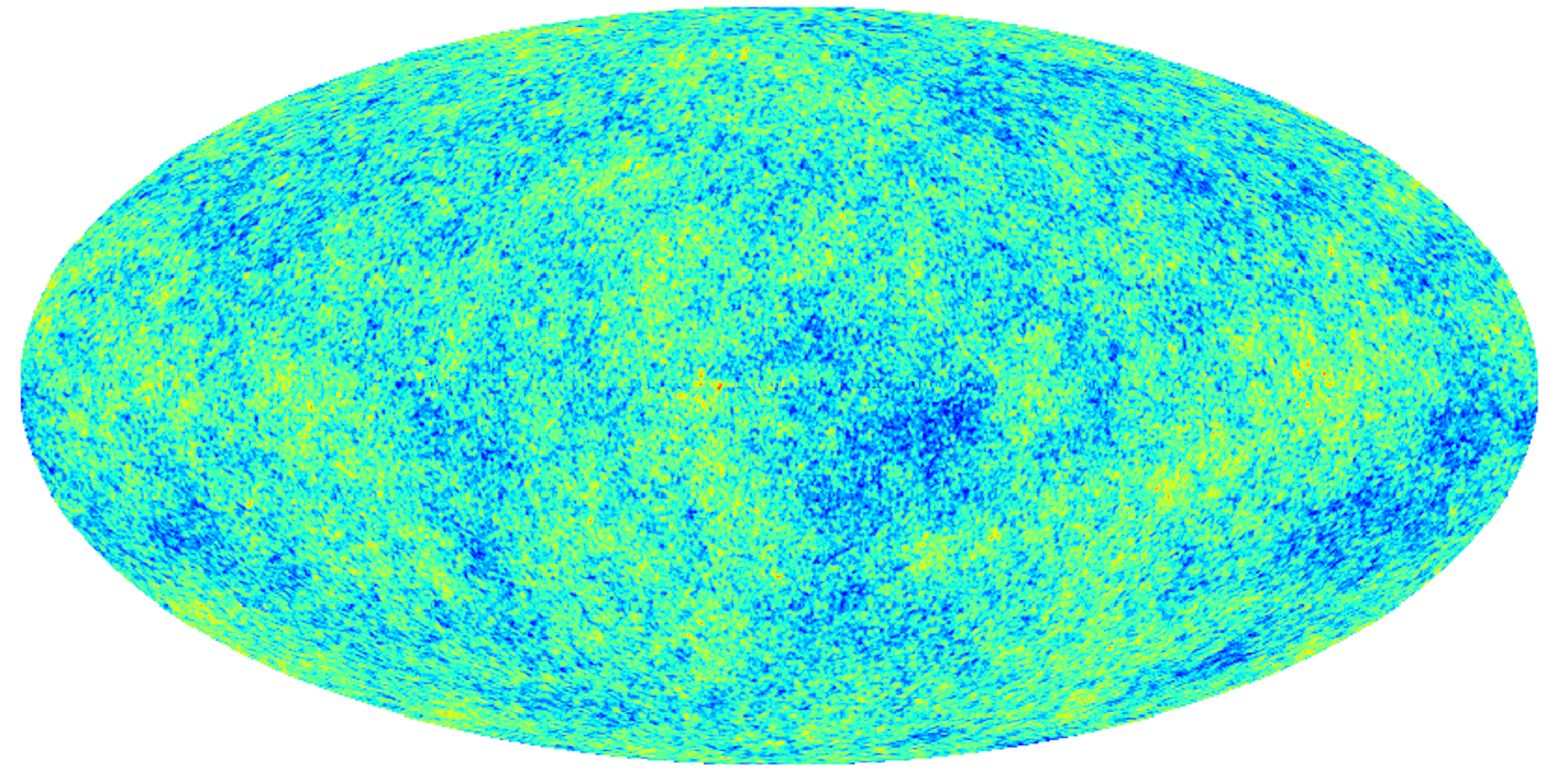
CMB data is directional, measuring fluctuations in radiation at a number of different frequencies, coming into a satellite from different directions. The first, satellite based, detailed measurement of the CMB was carried out by the Cosmic Microwave Background Explorer (COBE) probe in the early 1990’s, followed a decade later by the Wilkinson Microwave Anisotropy Probe (WMAP). Most recently, the high precision Planck mission was launched, which measured the temperature anisotropies of the CMB to an accuracy of $10^{-5}$ degrees. It measures the CMB temperature anisotropies at 7 different frequency bands, at a resolution of 5’ (i.e. 5 arc-minutes, or 5 sixtieth of a degree), representing the most detailed and precise measurement of the CMB temperature anisotropies till date. Common to all of these, however, is that each CMB measurement is that of a function on a sphere, as in Fig. 2.

Figure 2: A reconstructed version of CMB data from the Planck experiment, created using the Commander-Rule technique, seen in two dimensional, Mollweide projection.

There are many mathematical models for the CMB, the most common being that it is a realization of a homogeneous and isotropic Gaussian random field [43, 4, 45, 31, 35]. Both the assumptions of Gaussianity and homogeneity have been challenged recently, from both theoretical and empirical viewpoints [22, 34], and is the issue of homogeneity that we wish to address now, using PDs and Gibbs models. (The issue of Gaussianity is addressed in far more detail, using topological methods, albeit different to the ones that we are using here, in [39], and with geometrical methods in [37, 11].)

In order to test homogeneity, we first cut out a ring around the equator of $\pm 30^{\circ}$, leaving ‘northern’ and ‘southern’ $60^{\circ}$ spherical caps of data. The reason behind ignoring the central ring is that much of the ‘data’ here is not from actual observations, which are unavailable due to confounding effects such as the Milky Way, but is a ‘reconstruction’ using one of a variety of techniques [36]. Since all of these techniques are based on both Gaussian and homogeneity assumptions, the central ring should not show any deviation from the assumptions. Our aim is to test whether or not the CMB in the two caps can be assumed to be realizations of the same stochastic process.

The next step is to generate 8 smoothed version of the CMB in each cap, which we do with 8 different Gaussian kernels, with full width half maximum 300’, 180’, 120’, 90’, 60’, 40’, 20’ and 10’. The highest level of smoothing (300’) suppresses most of the fine scale variation seen in Fig. 2, while the 10’ level leads to no visually distinguishable difference. For each such smoothing, we produce PDs generated by the upper level set filtration, for both $H_{0}$ and $H_{1}$, leading to a total of $32=8\times 2\times 2$ PDs. Although the aims there are different, details of the numerical procedure can be found in [38], and an example of two PDs is given in Fig. 3.

Figure 3: $H_{1}$ persistence diagrams for unsmoothed CMB data, northern cap (left) and southern cap (right). There are approximately 27,000 points in each diagram.

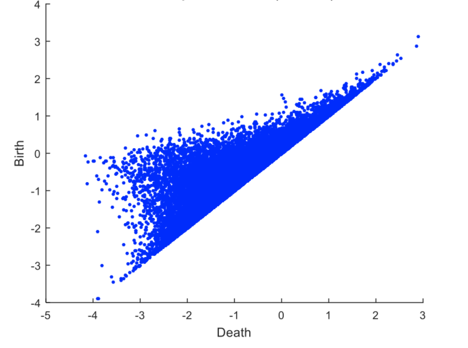
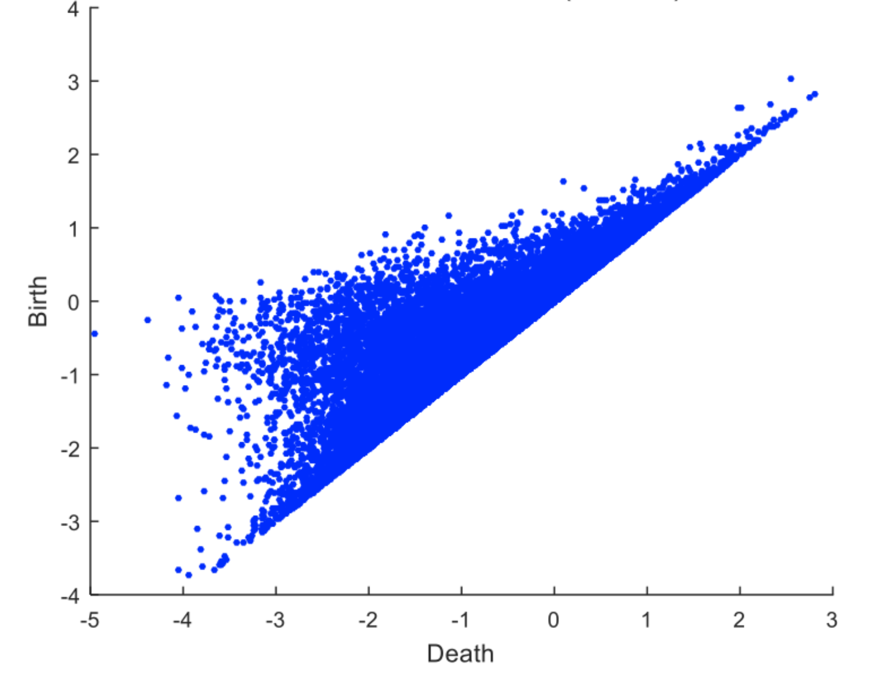
The two PDs of Fig. 3 are quite similar, and it is hard to see any obvious differences between them. However, fitting a Gibbs model with pseudolikelihood (5), again taking $K=2$, to each of our 32 PD yields some surprising results, summarized in Table 1.

Smoothing	300	180	120	90	60	40	20	10
$H_{0}$	0	1	3	3	3	3	5	1
$H_{1}$	0	0	3	2	2	3	5	5

Table 1: Number of north-south CMB parameter differences for difference smoothings and homologies. See text for details.

Each such model involves 5 free parameters (we treat $\delta$ as a nuisance parameter only), and Table 1 gives the number of such parameters that, for each smoothing, and for each PD ($H_{0}$ or $H_{1}$), were found to be significantly different between the models for the northern and southern caps. Significance was established using both the FDR method of [3] and the classical Bonferroni correction for multiple tests, both at a 5% significance level. (Both tests gave identical results.)

The results are quite striking. At the highest levels of smoothing, there is no evidence of a difference between the models for the PDs, regardless of homology. At the lower levels, the differences become more and more palpable. While we do not have a clear physical explanation for this, it is most likely due to the effect of interactions between objects that evolved due to the true primordial CMB fluctuations and foreground phenomena that evolved at later epochs.

However, whatever is the cosmological reason underlying Table 1, the implication is that it is unreasonable to assume that the northern and southern cap CMB maps are realizations of the same stochastic process. In other words, an hypothesis of homogeneity is not tenable.

From the point of view of this paper, however, our main discovery is not cosmological, but lies in demonstrating the ability of the Gibbs model, which assumes nothing about the original data, nor about how PDs express properties of the underlying data, to differentiate between complex structures using purely topological methods. Consequently, we believe that the approach described here will open the door to developing a wide variety of (semi-parametric) statistical methods for further applications of TDA.

6 Acknowledgments

Among others, we thank Jose Blanchet, Herbert Edelsbrunner, Jingchen Liu, Anthea Monod, Sayan Mukerjee, and Katherine Turner for helpful conversations in various stages of this research, which was supported in part by SATA II, AFOSR, FA9550-15-1-0032, and URSAT, ERC Advanced Grant 320422.

References

- [1] Aaron Adcock, Erik Carlsson, and Gunnar Carlsson. The ring of algebraic functions on persistence bar codes. Homology Homotopy Appl., 18(1):381–402, 2016.
- [2] Sudipto Banerjee, Bradley P. Carlin, and Alan E. Gelfand. Hierarchical modeling and analysis for spatial data, volume 135 of Monographs on Statistics and Applied Probability. CRC Press, Boca Raton, FL, second edition, 2015.
- [3] Yoav Benjamini and Yosef Hochberg. Controlling the false discovery rate: a practical and powerful approach to multiple testing. Journal of the Royal Statistical Society. Series B (Methodological), pages 289–300, 1995.
- [4] C. L. Bennett, M. Halpern, G. Hinshaw, and et. al. First-Year Wilkinson Microwave Anisotropy Probe (WMAP) Observations: Preliminary Maps and Basic Results. Astrophys. J. Suppl., 148:1–27, September 2003.
- [5] Julian Besag. Spatial interaction and the statistical analysis of lattice systems. J. Roy. Statist. Soc. Ser. B, 36:192–236, 1974. With discussion by D. R. Cox, A. G. Hawkes, P. Clifford, P. Whittle, K. Ord, R. Mead, J. M. Hammersley, and M. S. Bartlett and with a reply by the author.
- [6] O. Bobrowski, S. Mukherjee, and J.E. Taylor. Topological consistency via kernel estimation. Bernoulli, 2014. In print, arxiv:1407.5272.
- [7] Omer Bobrowski and Matthew Kahle. Topology of random geometric complexes: a survey. Preprint at http://arxiv. org/abs/1409.4734, 2014.
- [8] Omer Bobrowski, Matthew Kahle, and Primoz Skraba. Maximally persistent cycles in random geometric complexes. Annals of Applied Probability, 2017. In press, arxiv.org/abs/arXiv:1509.04347.
- [9] S. Brooks, A. Gemna, G.L. Jones, and X-L. Meng. Handbook of Markov Chain Monte Carlo. Chapman and Hall, Boca Raton, 2011.
- [10] Peter Bubenik. Statistical topological data analysis using persistence landscapes. Journal of Machine Learning Research, 16(1):77–102, 2015.
- [11] Thomas Buchert, Martin J. France, and Frank Steiner. Model-independent analyses of non-Gaussianity in Planck CMB maps using Minkowski Functionals. arxiv.org/abs/1701.03347, 2017.
- [12] Kenneth P. Burnham and David R. Anderson. Model Selection and Multimodel Inference. Springer-Verlag, New York, second edition, 2002. A practical information-theoretic approach.
- [13] G. Carlsson. Topology and data. Bull. Amer. Math. Soc. (N.S.), 46(2):255–308, 2009.
- [14] Gunnar Carlsson. Topological pattern recognition for point cloud data. Acta Numer., 23:289–368, 2014.
- [15] Bernard Chalmond. Modeling and Inverse Problems in Imaging Analysis, volume 155 of Applied Mathematical Sciences. Springer-Verlag, New York, 2003. Translated from the French, With a foreword by Henri Maître.
- [16] J.M. Chan, G. Carlsson, and P. Rabadan. Topology of viral evolution. Proceedings of the National Academy of Sciences, 110(46):18566–18571, 2013.
- [17] F. Chazal, B. T. Fasy, F. Lecci, B. Michel, A. Rinaldo, and L. Wasserman. Robust Topological Inference: Distance To a Measure and Kernel Distance. ArXiv e-prints, December 2014.
- [18] Carina Curto. What can topology tell us about the neural code? Bull. Amer. Math. Soc. (N.S.), 54(1):63–78, 2017.
- [19] Herbert Edelsbrunner. A short course in computational geometry and topology. Springer Briefs in Applied Sciences and Technology. Springer, Cham, 2014.
- [20] Herbert Edelsbrunner and John Harer. Persistent homology—a survey. In Surveys on discrete and computational geometry, volume 453 of Contemp. Math., pages 257–282. Amer. Math. Soc., Providence, RI, 2008.
- [21] Herbert Edelsbrunner and John L. Harer. Computational topology. American Mathematical Society, Providence, RI, 2010. An introduction.
- [22] H. K. Eriksen, F. K. Hansen, A. J. Banday, K. M. Gorski, and P. B. Lilje. Asymmetries in the cosmic microwave background anisotropy field. The Astrophysical Journal, 605(1):14, 2004.
- [23] Brittany Terese Fasy, Fabrizio Lecci, Alessandro Rinaldo, Larry Wasserman, Sivaraman Balakrishnan, and Aarti Singh. Confidence sets for persistence diagrams. Ann. Statist., 42(6):2301–2339, 2014.
- [24] Hans-Otto Georgii. Gibbs Measures and Phase Transitions, volume 9 of de Gruyter Studies in Mathematics. Walter de Gruyter & Co., Berlin, second edition, 2011.
- [25] R. Ghrist. Barcodes: the persistent topology of data. Bull. Amer. Math. Soc. (N.S.), 45(1):61–75 (electronic), 2008.
- [26] Robert Ghrist. Elementary Applied Topology. Createspace, 2014.
- [27] C. Giusti, E. Pastalkova, C. Curto, and V. Itskov. Clique topology reveals intrinsic geometric structure in neural correlations. Proceedings of the National Academy of Sciences, 112(44):13455–13460, 2015.
- [28] Yasuaki Hiraoka, Takenobu Nakamura, Akihiko Hirata, Emerson G. Escolar, Kaname Matsue, and Yasumasa Nishiura. Hierarchical structures of amorphous solids characterized by persistent homology. PNAS, 113:7035–7040, 2016.
- [29] Matthew Kahle. Topology of random simplicial complexes: a survey. In Algebraic topology: applications and new directions, volume 620 of Contemp. Math., pages 201–221. Amer. Math. Soc., Providence, RI, 2014.
- [30] James M. Kilner and Karl J. Friston. Topological inference for EEG and MEG. Ann. Appl. Stat., 4(3):1272–1290, 2010.
- [31] E. Komatsu et al. Seven-year Wilkinson Microwave Anisotropy Probe (WMAP) Observations: Cosmological Interpretation. Astrophysical Journal Supplement Series, 2011.
- [32] Elizabeth Munch, Katharine Turner, Paul Bendich, Sayan Mukherjee, Jonathan Mattingly, and John Harer. Probabilistic Fréchet means for time varying persistence diagrams. Electron. J. Stat., 9(1):1173–1204, 2015.
- [33] M. Nicolau, A.J. Levine, and G. Carlsson. Topology based data analysis identifies a subgroup of breast cancers with a unique mutational profile and excellent survival. Proceedings of the National Academy of Sciences, 108(17):7265–7270, 2011.
- [34] Chan-Gyung Park. Non-Gaussian signatures in the temperature fluctuation observed by the Wilkinson Microwave Anisotropy Probe. Monthly Notices of the Royal Astronomical Society, 349(1):313–320, 2004.
- [35] Planck Collaboration, P. A. R. Ade, N. Aghanim, M. Arnaud, M. Ashdown, J. Aumont, C. Baccigalupi, A. J. Banday, R. B. Barreiro, J. G. Bartlett, and et al. Planck 2015 results. XIII. Cosmological parameters. ArXiv e-prints, February 2015.
- [36] Plank Collaboration:, Peter AR Ade, and et al. Planck 2013 results. XII. Diffuse component separation. Astronomy & Astrophysics, 571:A12, 2014.
- [37] Plank Collaboration:, Peter AR Ade, and et al. Planck 2015 results. XVI. Isotropy and statistics of the CMB. Astronomy & Astrophysics, 594:A16, 2016.
- [38] P. Pranav, H. Edelsbrunner, R. van de Weygaert, G. Vegter, M. Kerber, B. J. T. Jones, and M. Wintraecken. The topology of the cosmic web in terms of persistent Betti numbers. Monthly Notices of the Royal Astronomical Society, 465:4281–4310, March 2017.
- [39] Pratyush Pranav, Robert Adler, Herbert Edelsbrunner, Bernard J.T. Jones, Hubert Wagner, and Rien van de Weygaert3Bobrowski. Loops in the cosmic microwave background. 2017. In preparation.
- [40] Christian P. Robert and George Casella. Monte Carlo Statistical Methods. Springer Texts in Statistics. Springer-Verlag, New York, second edition, 2004.
- [41] A. Robinson and K. Turner. Hypothesis Testing for Topological Data Analysis. ArXiv e-prints, October 2013.
- [42] Andrew Robinson and Katharine Turner. Hypothesis testing for topological data analysis. 2017. arxiv.org/abs/arXiv:1301.7467.
- [43] G. F. Smoot, C. L. Bennett, A. Kogut, and et. al. Structure in the COBE differential microwave radiometer first-year maps. Astrophys.J.Lett., 396:L1–L5, September 1992.
- [44] Thierry Sousbie. The persistent cosmic web and its filamentary structure–i. theory and implementation. Monthly Notices of the Royal Astronomical Society, 414(1):350–383, 2011.
- [45] D. N. Spergel, R. Bean, O. Doré, and et. al. Three-Year Wilkinson Microwave Anisotropy Probe (WMAP) Observations: Implications for Cosmology. Astrophys.J.Suppl., 170:377–408, June 2007.
- [46] John W. Tukey. The future of data analysis. Ann. Math. Statist., 33:1–67, 1962.
- [47] Katharine Turner, Yuriy Mileyko, Sayan Mukherjee, and John Harer. Fréchet means for distributions of persistence diagrams. Discrete Comput. Geom., 52(1):44–70, 2014.
- [48] Larry Wasserman. Topological data analysis. 2016. In preparation.