Gravitational allocation for uniform points on the sphere

Abstract

Given a collection $\mathcal{L}$ of $n$ points on a sphere $\mathbf{S}^{2}_{n}$ of surface area $n$, a fair allocation is a partition of the sphere into $n$ cells each of area $1$, and each associated with a distinct point of $\mathcal{L}$. We show that if the $n$ points are chosen uniformly at random and the partition is defined by considering a “gravitational” potential defined by the $n$ points, then the expected distance between a point on the sphere and the associated point of $\mathcal{L}$ is $O(\sqrt{\log n})$. We use our result to define a matching between two collections of $n$ independent and uniform points on the sphere and prove that the expected distance between a pair of matched points is $O(\sqrt{\log n})$, which is optimal by a result of Ajtai, Komlós, and Tusnády. Furthermore, we prove that the expected number of maxima for the gravitational potential is $\Theta(n/\log n)$. We also study gravitational allocation on the sphere to the zero set $\mathcal{L}$ of a particular Gaussian polynomial, and we quantify the repulsion between the points of $\mathcal{L}$ by proving that the expected distance between a point on the sphere and the associated point of $\mathcal{L}$ is $O(1)$.

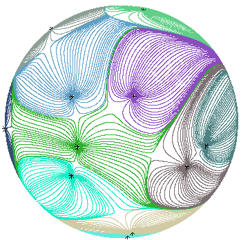
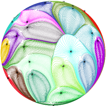
Figure 1: Gravitational allocation to $n$ uniform and independent points on a sphere with $n=15$ and $n=40$. The basin of attraction of each point has equal area.

1 Introduction

Let $n$ be a positive integer, and let $\mathbf{S}^{2}_{n}\subset\mathbf{R}^{3}$ be the sphere centered at the origin with radius chosen such that with $\lambda_{n}$ denoting surface area we have $\lambda_{n}(\mathbf{S}^{2}_{n})=n$. For any set $\mathcal{L}\subset\mathbf{S}^{2}_{n}$ consisting of $n$ points, we say that a measurable function $\psi:\mathbf{S}^{2}_{n}\to\mathcal{L}\cup\{\infty\}$ is a fair allocation of $\lambda_{n}$ to $\mathcal{L}$ if it satisfies the following:

$$\lambda_{n}(\psi^{-1}(\infty))=0,\qquad\qquad\lambda_{n}(\psi^{-1}(z))=1,\quad\forall z\in\mathcal{L}.$$ (1.1)

For $z\in\mathcal{L}$ we call $\psi^{-1}(z)$ the cell allocated to $z$. In other words, a fair allocation is a way to divide $\mathbf{S}^{2}_{n}$ into $n$ cells of measure 1 (up to a set of measure 0), with each cell associated to a distinct point of $\mathcal{L}$.

Let $\mathcal{L}$ be a random collection of $n$ points on $\mathbf{S}^{2}_{n}$ which is invariant in law under rotations of the sphere, i.e., $\phi(\mathcal{L})$ has the same law as $\mathcal{L}$ for any rotation $\phi:\mathbf{S}^{2}_{n}\to\mathbf{S}^{2}_{n}$. An allocation rule is a measurable map $\mathcal{L}\mapsto\psi_{\mathcal{L}}$ which is defined almost surely with respect to the randomness of $\mathcal{L}$, such that (i) $\psi_{\mathcal{L}}$ is a fair allocation of $\lambda_{n}$ to $\mathcal{L}$, and (ii) the map $\mathcal{L}\mapsto\psi_{\mathcal{L}}$ is rotation-equivariant. The latter property means that for any rotation $\phi$ and almost every $x\in\mathbf{S}^{2}_{n}$, we have $\psi_{\phi(\mathcal{L})}(\phi(x))=\phi(\psi_{\mathcal{L}}(x))$.

Gravitational allocation is a particular allocation rule based on treating points in $\mathcal{L}$ as wells of a potential function. The cell allocated to $z\in\mathcal{L}$ is then taken to be the basin of attraction of $z$ with respect to the flow induced by the negative gradient of this potential. When the potential takes a particular form which mimics the gravitational potential of Newtonian mechanics, it is ensured that a.s. each cell has area $1$. In this paper we will mainly consider gravitational allocation on the sphere for the case when $\mathcal{L}$ is a set of $n$ points chosen uniformly and independently at random from $\mathbf{S}^{2}_{n}$.

Let us now define gravitational allocation precisely. Consider the potential $U:\mathbf{S}_{n}^{2}\to\mathbf{R}$ given by

$$U(x)=\sum_{z\in\mathcal{L}}\log|x-z|,$$ (1.2)

where $|\cdot|$ denotes Euclidean distance in $\mathbf{R}^{3}$. For each location $x\in\mathbf{S}^{2}_{n}$, let $F(x)$ denote the negative gradient of $U$ with respect to the usual spherical metric (i.e., the one induced from $\mathbf{R}^{3}$). Note that $F(x)$ is an element of the tangent space at $x\in\mathbf{S}^{2}_{n}$, and we think of it as describing the “force” on $x$ arising from the potential $U$.

For any $x\in\mathbf{S}^{2}_{n}$ consider the integral curve $Y_{x}(t)$ defined by

$$\frac{dY_{x}}{dt}(t)=F(Y_{x}(t)),\qquad Y_{x}(0)=x.$$ (1.3)

Since $F$ is smooth away from $\mathcal{L}$, by standard results about flows on vector fields (see e.g. the proof of Lemma 17.10 in [Lee03]), for each fixed $x\in\mathbf{S}^{2}_{n}$ the curve $Y_{x}$ can be defined over some maximal domain $(-\infty,\tau_{x})$, where $0<\tau_{x}\leq\infty$. Note that the force $F$ represents the speed of a particle, rather than being proportional to its acceleration as in Newtonian gravitation.

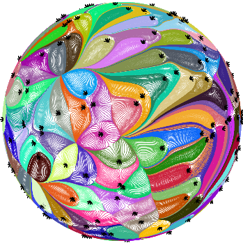
Figure 2: Gravitational allocation to $n$ uniform and independent points with $n=200$ and $n=750$ (see Figure 1 for smaller $n$). The basins become more elongated as $n$ grows, reflecting Theorem 2. The MATLAB script used to generated these figures is based on code written by M. Krishnapur.

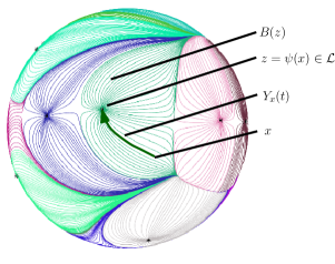
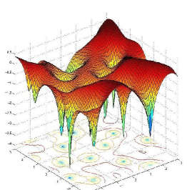
Figure 3: Left: Illustration of $Y_{x}$, $B(z)$, and $\psi(x)$ for $x\in\mathbf{S}^{2}_{n}$ and $z\in\mathcal{L}$. Right: Gravitational potential, by M. Krishnapur.

We then define gravitational allocation on the sphere to be the allocation rule given by

$$\psi(x)=\begin{cases}z&\qquad\text{if\,\,}\lim_{t\uparrow\tau_{x}}Y_{x}(t)=z\text{\,\,\,and\,\,\,}z\in\mathcal{L},\\ \infty&\qquad\text{otherwise.}\end{cases}$$ (1.4)

For $z\in\mathcal{L}$, the set

$$B(z)=\left\{x\in\mathbf{S}^{2}_{n}\,:\,\psi(x)=z\right\}$$ (1.5)

of points allocated to $z$ will be called its basin of attraction.

It turns out, as stated in the following proposition, that each basin of attraction almost surely has unit area, so that (1.4) indeed gives rise to a fair allocation.

Proposition 1.

For $n\in\mathbbm{N}$ let $\mathbf{S}^{2}_{n}$ be the sphere centered at the origin with surface area $n$, and let $\mathcal{L}\subset\mathbf{S}^{2}_{n}$ be a set of $n$ distinct points. The function $\psi$ given by (1.4) defines a fair allocation of $\lambda_{n}$ to $\mathcal{L}$.

The proof of Proposition 1 is given in Section 2. We are now ready to state the main results of this paper.

1.1 Statement of main results

Our first main result estimates the average distance between a point $x$ and the point $\psi(x)$ it is allocated to.

Theorem 2.

Let $n\in\{2,3,\dots\}$. Consider any $x\in\mathbf{S}^{2}_{n}$, and let $\mathcal{L}\subset\mathbf{S}^{2}_{n}$ be a collection of $n$ points chosen uniformly and independently at random from $\mathbf{S}^{2}_{n}$. For any $p>0$ there is a constant $C>0$ depending only on $p$ such that for $r>0$,

$$\mathbf{P}\left[|\psi(x)-x|>r\sqrt{{\log n}}\right]\leq Cr^{-p}.$$ (1.6)

In particular, for some universal constant $C>0$,

$$\mathbf{E}[|\psi(x)-x|]\leq C\sqrt{\log n}.$$ (1.7)

Gravitational allocation is optimal in the sense that (1.7) cannot be improved by more than a constant factor for other allocation rules for uniform and independent points (see Remark 9).

We remark that one may obtain the bound (1.7) (without the tail estimate (1.6)) more directly via the following identity, which is of independent interest and also applied in the proof of Proposition 6 stated below.

$$\frac{1}{n}\int_{\mathbf{S}^{2}_{n}}\int_{0}^{\tau_{x}}|F(Y_{x}(t))|\,dt\,d\lambda_{n}(x)=\frac{1}{2\pi n}\int_{\mathbf{S}^{2}_{n}}|F(x)|\,d\lambda_{n}(x).$$ (1.8)

Taking the expectation over $\mathcal{L}$, the left side upper bounds the average value of $|\psi(x)-x|$, while the right side can be shown to be $O(\sqrt{\log n})$ using simpler versions of estimates carried out in Section 4. We give the short proof of (1.8) in Section 2.

Fair allocations are closely related to distance-minimizing perfect matchings between sets of points. For example, we have the following corollary of (1.7). See Section 1.3 for two short proofs.

Corollary 3.

For $n\in\{2,3,\dots\}$ consider two sets of $n$ points $\mathcal{A}=\{a_{1},\dots,a_{n}\}$ and $\mathcal{B}=\{b_{1},\dots,b_{n}\}$ sampled uniformly and independently at random from $\mathbf{S}^{2}_{n}$. We can define a matching $\varphi$ of $\mathcal{A}$ and $\mathcal{B}$ (i.e., a bijection $\varphi:\mathcal{A}\to\mathcal{B}$) using gravitational allocation, such that for some universal constant $C$,

$$\mathbf{E}\left[\frac{1}{n}\sum_{k=1}^{n}|\varphi(a_{k})-a_{k}|\right]\leq C\sqrt{\log n}.$$

The next theorem shows that the expected number of local maxima of the potential $U$ is of order $\frac{n}{\log n}$. The theorem addresses a question of Nazarov, Sodin, and Volberg [NSV07, Question 12.6], who, in the context of gravitational allocation to the zero set of a Gaussian analytic function, ask about properties of the graph whose vertices are maxima for the potential $U$ and whose edges formed by allocation cell boundaries.

Theorem 4.

If $N\in\mathbbm{N}\cup\{\infty\}$ denotes the number of local maxima of $U$, then for some universal constant $C>0$ we have

$$\frac{n}{C\log n}\leq\mathbf{E}[N]\leq\frac{Cn}{\log n}.$$

As a corollary to Theorem 4 we can deduce that the typical basin diameter is at least of order $\sqrt{\log n}$.

Corollary 5.

For any $\varepsilon>0$ there exists a $\delta>0$ such that for any fixed $x\in\mathbf{S}^{2}_{n}$, with probability at least $1-\varepsilon$, the cell containing $x$ has diameter at least $\delta\sqrt{\log n}$.

Note that (1.7) from Theorem 2 also gives a lower bound on $|\psi(x)-x|$. However, the bound is only for the expectation, allowing for the possibility that $|\psi(x)-x|$ is usually of constant order but takes very large values with a small probability. Corollary 5 rules out this possibility. The short proof is deferred to Section 1.4.

As mentioned above, the bound (1.7) is optimal among all allocation rules up to multiplication by a constant for the case where the points of $\mathcal{L}$ are uniform and independent. However, there exist other rotationally equivariant point processes that are spread more evenly over the sphere, and in these cases it is possible to have $\mathbf{E}[|\psi(x)-x|]=O(1)$. We now introduce one such process constructed by taking the roots of a certain random Gaussian polynomial. Specifically, we look at the polynomial

$$p(z)=\sum_{k=0}^{n}\zeta_{k}\frac{\sqrt{n(n-1)\cdots(n-k+1)}}{\sqrt{k!}}z^{k},$$ (1.9)

where $\zeta_{1},\ldots,\zeta_{n}$ are independent standard complex Gaussians. The roots $\lambda_{1},\ldots,\lambda_{n}$ of $p$ are then $n$ random points in the complex plane, which we can bring to the sphere via stereographic projection in such a way that

$$\mathcal{L}=\left\{P_{n}^{-1}(\sqrt{n}\lambda_{k})\right\}_{k=1}^{n}$$

is a rotationally equivariant random set of $n$ points on $\mathbf{S}^{2}_{n}$ (see Section 8 for details). Heuristically, the points of $\mathcal{L}$ are distributed more evenly than independent uniformly random points, because roots of random polynomials tend to “repel” each other (see Fig. 4). This can be quantified as follows.

Proposition 6.

Let $\psi:\mathbf{S}^{2}_{n}\to\mathcal{L}$ be the gravitational allocation to $\mathcal{L}$. Then,

$$\mathbf{E}\bigg{[}\frac{1}{n}\int_{\mathbf{S}^{2}_{n}}|x-\psi(x)|d\lambda_{n}(x)\bigg{]}\leq\frac{\sqrt{\pi}}{4}.$$ (1.10)

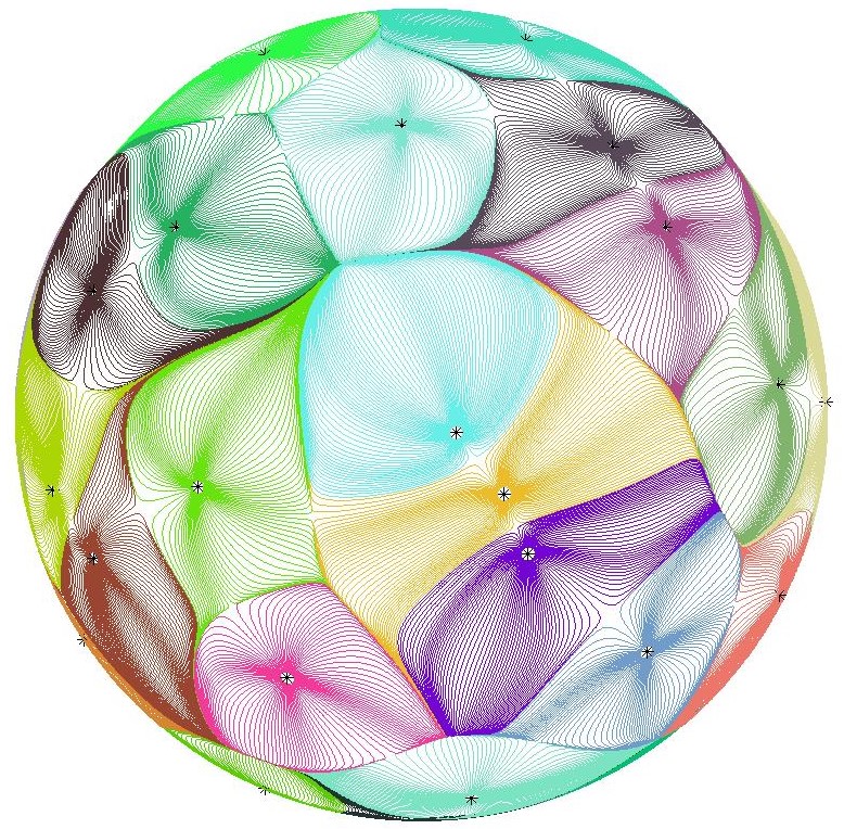
Figure 4: A simulation of gravitational allocation to the zeroes of the Gaussian random polynomial (1.9). The cells are evenly proportioned, in contrast with the more elongated shapes seen in Figure 2. The simulation was made by R. Peled and J. Ding, based on code by M. Krishnapur.

1.2 Related work on allocations

Nazarov, Sodin, and Volberg [NSV07] analyzed a fair allocation to the zeros of a certain Gaussian entire function $g$, obtained from the gradient flow determined by the potential $U=\log|g|-\frac{1}{2}|z|^{2}$. The term “gravitational allocation” was introduced by Chatterjee, Peled, Peres, and Romik [CPPR10a], who considered gravitational allocation to the points $\mathcal{L}\subset\mathbf{R}^{d}$ of a unit intensity Poisson point process (PPP) for $d\geq 3$. Both papers [NSV07] and [CPPR10a] prove an exponential tail (with a small correction for the PPP when $d=3$) for the diameter of the cell containing the origin. Phase transitions for the cells of gravitational allocation to a PPP in $\mathbf{R}^{d}$ were studied in [CPPR10b].

The gravitational allocation for a PPP in $\mathbf{R}^{d}$ as studied in [CPPR10a] is not well-defined for $d=2$ because the sum defining the force is divergent. Indeed, a lower bound for $d\leq 2$ was given in [HP05] (based on results from [HL01, Lig02]): any allocation rule for a PPP in $\mathbf{R}^{d}$ with $d=1,2$ satisfies $\mathbf{E}[X^{d/2}]=\infty$, where $X$ is the distance between the origin and the point it is allocated to. Nevertheless, one can study the behavior of gravitational allocation in two dimensions by considering a finite version of the problem, which motivates our present setting of taking finitely many points on the sphere. Our quantitative bounds are consistent with [HL01], because the average distance (after appropriate scaling) grows as $\sqrt{\log n}$ with the number of points $n$.

Gravitational allocation can also be viewed as an instantiation of the Dacorogna-Moser [DM90] scheme for a general Riemannian manifold $D$ with volume measure $\mathfrak{m}$. This scheme provides (under certain smoothness assumptions) a coupling $\pi$ between probability measures $\rho_{0}\mathfrak{m}$ and $\rho_{1}\mathfrak{m}$ by solving the PDE $\Delta u=\rho_{0}-\rho_{1}$ and then considering the flow for the vector field $-\nabla u$. The coupling $\pi$ is deterministic (i.e., if $(X,Y)\sim\pi$ for $X\sim\rho_{0}\mathfrak{m}$ and $Y\sim\rho_{1}\mathfrak{m}$ then $Y$ is a deterministic function of $X$), and is called a transport map for this reason.

It was observed by Caracciolo, Lucibello, Parisi, and Sicuro [CLPS14] that the differential equation $\Delta u=\rho_{0}-\rho_{1}$ may be seen as a linearization of the Monge-Ampère equation, which describes the optimal transportation map for the Wasserstein 2-distance. Based on this, they predicted the leading order asymptotic term for optimal quadratic allocation in $2$-dimensions (in addition to related predictions for higher dimensions). The $2$-dimensional prediction was recently confirmed by Ambrosio, Stra, and Trevisan [AST16] for optimal quadratic allocation cost to i.i.d. points sampled from a $2$-dimensional Riemannian manifold. However, they do not obtain their result by studying an explicit allocation method, but via a duality argument. Finer estimates with simpler proofs, for more general manifolds, and with sharper error bounds were obtained by Ambrosio and Glaudo [AG18].

Earlier works have also studied other allocation rules besides gravitational allocation. The stable marriage allocation [HHP06, HHP09] can be defined for every translation-invariant point process with unit intensity in $\mathbf{R}^{d}$ for $d\geq 1$: it is the unique allocation which is stable in the sense of the Gale-Shapley marriage problem. With this allocation, a.s. all cells are open and bounded, but not necessarily connected. Allocation rules for a PPP in $\mathbf{R}^{d}$ which minimize transportation cost per unit mass were considered in [HS13] with various cost functions, using tools from optimal transportation.

We remark that the results of the current paper were announced in the work [HPZ18] by the same authors.

1.3 Matchings: Proof of Corollary 3 and related works

In this section we will give two short alternative proofs of Corollary 3, and then discuss other results on matchings.

Proof of Corollary 3 using online matching algorithm.

Consider the gravitational allocation $\psi$ to the point set $\mathcal{B}$, and set $\varphi(a_{1})=\psi(a_{1})$, so that Theorem 2 gives

$$\mathbf{E}[|\varphi(a_{1})-a_{1}|]\leq C\sqrt{\log n}.$$

Define

$$\mathcal{A}^{\prime}:=\{a_{2},\ldots,a_{n}\},\qquad\mathcal{B}^{\prime}:=\mathcal{B}\setminus\{\psi(a_{1})\}.$$

Note that since $\psi$ is a fair allocation, $\psi(a_{1})$ is uniformly distributed over elements of $\mathcal{B}$ (under the randomness of $a_{1}$). Thus $\mathcal{A}^{\prime}$ and $\mathcal{B}^{\prime}$ both have the law of $n-1$ points chosen independently and uniformly at random from $\mathbf{S}^{2}_{n}$. Also, it is clear that $\mathcal{A}^{\prime}$ and $\mathcal{B}^{\prime}$ are independent. Hence, we may repeat the same procedure with the sets $\mathcal{A}^{\prime}$ and $\mathcal{B}^{\prime}$ to define $\varphi(a_{2})$, and we bound $|\varphi(a_{2})-a_{2}|$ using Theorem 2 with $n-1$ points. (However, note that our matching algorithm for $n-1$ points occurs on $\mathbf{S}^{2}_{n-1}$, so we must rescale by a multiplicative factor $\sqrt{\frac{n}{n-1}}$.) Repeating this procedure, it follows that

$$\mathbf{E}\left[\frac{1}{n}\sum_{k=1}^{n}|\varphi(a_{k})-a_{k}|\right]\leq\frac{C}{n}\sum_{k=1}^{n}\sqrt{\frac{n}{k}}\sqrt{\log(k\vee 2)}\leq 2C\log n.$$

∎

Proof of Corollary 3 using the Birkhoff-von Neumann Theorem.

Let $\psi_{\mathcal{A}}$ and $\psi_{\mathcal{B}}$ describe gravitational allocation to $\mathcal{A}$ and $\mathcal{B}$, respectively. Then, we can form a coupling between the uniform distributions on $\mathcal{A}$ and $\mathcal{B}$ as follows: we sample $(a,b)\in\mathcal{A}\times\mathcal{B}$ by drawing $X$ uniformly at random from $\mathbf{S}_{n}^{2}$ and setting $a=\psi_{\mathcal{A}}(X)$ and $b=\psi_{\mathcal{B}}(X)$.

We have by Theorem 2 that the expected coupling distance satisfies the bound

$$\mathbf{E}|a-b|\leq\mathbf{E}|a-X|+\mathbf{E}|b-X|\leq 2C\sqrt{\log n}.$$ (1.11)

By the Birkhoff-von Neumann theorem (see e.g. [vLW01, Theorem 5.5]), any coupling between two uniform distributions on $n$ elements is a mixture of deterministic matchings between the two sample spaces. Thus, there exists some matching between $\mathcal{A}$ and $\mathcal{B}$ whose average matching distance is upper bounded by the quantity in (1.11), i.e., the average matching distance is of order $\sqrt{\log n}$. ∎

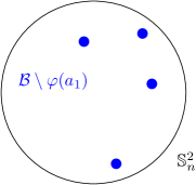
Figure 5: Illustration of the proof of Corollary 3. The set $\mathcal{B}\setminus\varphi(a_{1})$ consists of $n-1$ uniform and independent points on the sphere $\mathbf{S}_{n}^{2}$ of area $n$.

Remark 7.

Each proof of the corollary gives a general procedure for obtaining a matching from an allocation rule. In particular, we see from the second proof that if $\mathcal{A},\mathcal{B}\subset\mathbf{S}^{2}_{n}$ are two sets of $n$ points, and $\psi_{\mathcal{A}}$ and $\psi_{\mathcal{B}}$ are fair allocations of $\lambda_{n}$ to $\mathcal{A}$ and $\mathcal{B}$, respectively, then there exists a matching $\varphi:\mathcal{A}\to\mathcal{B}$ such that

$$\sum_{a\in\mathcal{A}}|a-\varphi(a)|\leq\int_{\mathbf{S}^{2}_{n}}\!\!|x-\psi_{\mathcal{A}}(x)|d\lambda_{n}(x)+\int_{\mathbf{S}^{2}_{n}}\!\!|x-\psi_{\mathcal{B}}(x)|d\lambda_{n}(x).$$ (1.12)

Minimal matchings of random points in the plane have been extensively studied (see e.g. [AKT84, LS89, Tal94, Tal14]). The asymptotic behavior of the minimal average matching distance was identified in [AKT84]: it was shown that for two sets $\mathcal{A}$ and $\mathcal{B}$ of $n$ i.i.d. uniformly chosen points from $[0,\sqrt{n}]^{2}$, there exist constants $C_{1},C_{2}>0$ such that

$$\lim_{n\rightarrow\infty}\mathbf{P}\left(C_{1}\sqrt{\log n}\leq\frac{1}{n}\min_{\begin{subarray}{c}\varphi:\mathcal{A}\to\mathcal{B}\\ \text{bijective}\end{subarray}}\sum_{a\in\mathcal{A}}|\varphi(a)-a|\leq C_{2}\sqrt{\log n}\right)=1.$$

In the limit as $n\rightarrow\infty$, one expects minimal matching on the sphere to be essentially equivalent to minimal matching in a square, as the local geometries are the same to first order. Indeed, we give a formal statement of one direction of this equivalence in the next proposition, which is proved in Section 6.

Proposition 8.

Consider any integer $n\geq 2$, and write $N=n^{2}$. Suppose that $\mathcal{X}$ and $\mathcal{Y}$ are two sets of $N$ i.i.d. uniformly random points from $\mathbf{S}^{2}_{N}$, and $\mathcal{A}$ and $\mathcal{B}$ are two sets of $n$ i.i.d. uniformly random points from $[0,\sqrt{n}]^{2}$. Then, for a universal constant $C$,

$$\frac{1}{n}\mathbf{E}\min_{\begin{subarray}{c}\varphi:\mathcal{A}\to B\\ \text{bijective}\end{subarray}}\;\sum_{a\in\mathcal{A}}|\varphi(a)-a|\leq C+\frac{C}{N}\cdot\mathbf{E}\min_{\begin{subarray}{c}\varphi:\mathcal{X}\to\mathcal{Y}\\ \text{bijective}\end{subarray}}\;\sum_{x\in\mathcal{X}}|\varphi(x)-x|.$$

Remark 9.

Combined with [AKT84], Proposition 8 implies that the bound of Corollary 3 is optimal up to multiplication by a constant. Using (1.12), we further get that gravitational allocation is optimal in the sense that the bound (1.7) cannot be better for other allocation rules.

Leighton and Shor studied the optimal maximal matching distance for uniform points in the square. The lower bound derived in [Sho85, Sho86] and the upper bound derived in [LS89] show that for two sets $\mathcal{A}$ and $\mathcal{B}$ of $n$ i.i.d. uniformly chosen points from $[0,\sqrt{n}]^{2}$, there exist constants $C_{1},C_{2}>0$ such that

$$\lim_{n\rightarrow\infty}\mathbf{P}\left(C_{1}(\log n)^{3/4}\leq\min_{\begin{subarray}{c}\varphi:\mathcal{A}\to\mathcal{B}\\ \text{bijective}\end{subarray}}\max_{a\in\mathcal{A}}|\varphi(a)-a|\leq C_{2}(\log n)^{3/4}\right)=1.$$

The maximal travel distance for the matching algorithm used in the first proof of Corollary 3 is of order $\sqrt{n}$, as compared to $(\log n)^{3/4}$ for the optimal matching. However, note that our matching algorithm is online, meaning that the points of $\mathcal{A}$ are revealed one by one, and we have to match a given point of $\mathcal{A}$ to a point of $\mathcal{B}$ before revealing the remaining points of $\mathcal{A}$. The typical maximal travel distance will always be of order $\sqrt{n}$ for online matching algorithms.

The allocation and matching problems for uniform points have also been studied for domains of dimension $d$ not necessarily equal to $2$, and with cost function given by the $p$-th power of the distance for $p\geq 1$. Asymptotic results for the optimal allocation or matching have been obtained for $d=1$ or $2$ and all $p\geq 1$ [CS14, AKT84] as well as for $d\geq 3$ and certain $p\geq 1$ [BdMM02, DY95, BB13, FG15].

1.4 Proof outline for distance bound (Theorem 2) and a heuristic picture

In order to bound $|\psi(x)-x|$ we will bound separately the duration $\tau_{x}$ of the flow $Y_{x}$ and its speed $|F(Y_{x}(t))|$ for $t\in(0,\tau_{x})$. The probability distribution of $\tau_{x}$ may be calculated exactly using Liouville’s theorem (Proposition 11) and turns out to be exponential (with a constant mean independent of $n$).

It remains to control $|F(y)|$, which turns out to be of order $\sqrt{\log n}$. If it is always less than $\sqrt{\log n}$, then combining with the tail bounds for $\tau_{x}$ yields the theorem. However, this is not precisely the case, as $|F(y)|$ can be very large if $y$ is close to a point in $\mathcal{L}$. We show in Section 5 that the contribution to $|F(y)|$ coming from points in $\mathcal{L}$ outside a ball centered at $y$ of radius $\Theta(1/\sqrt{\log n})$ is very unlikely to exceed $C\sqrt{\log n}$ for $C\gg 1$. Therefore, if $|F(y)|\gg C\sqrt{\log n}$, the main contribution to the force is most likely coming from points of $\mathcal{L}$ rather close to $y$. In that case, we argue (see Lemma 20) that one of these nearby points typically is the point of attraction for $y$ under the gravitational flow, which gives a bound for the distance traveled when $|F(y)|$ is large.

The simulations in Figure 2 suggest that the cells formed by gravitational allocation on the sphere are long and thin. This qualitative picture is depicted in Figure 6, and the accompanying description gives a heuristic argument along the lines of our proof outline above for why this is the case.

Figure 6: The figure gives a heuristic argument justifying Theorem 2. Since the “force” $F$ is typically of order $\sqrt{\log n}$ and the force exerted by a point at distance $d$ has magnitude of order $1/d$, the force exerted on a particle is dominated by the forces from far away points, except if there is a point of $\mathcal{L}$ at distance of order $1/\sqrt{\log n}$ or less. The probability that there are no points in a strip of width $1/\sqrt{\log n}$ and length $R\sqrt{\log n}$ decays exponentially in $R$, which suggests (heuristically) that the probability of traveling further than $R\sqrt{\log n}$ should be smaller than $\exp(-cR)$ for some $c>0$.

Finally we provide the proof of Corollary 5 upon an application of Theorem 4.

Proof of Corollary 5.

Let $E$ be the event that there are less than $Cn/\log n$ local maxima, where $C$ is a constant depending only on $\varepsilon$ that is chosen large enough so that $\mathbf{P}(E)\geq 1-\varepsilon/2$ (this is possible by Markov’s inequality and Theorem 4).

Let $R=\sqrt{\frac{(\log n)\varepsilon}{2C\pi}}$, and note that for each local maximum, the spherical cap of radius $R$ centered at that maximum has area less than $\pi R^{2}=\frac{\varepsilon\log n}{2C}$. Thus, on the event $E$, the total area of points on the sphere within distance $R$ of a local maximum is at most

$$\frac{Cn}{\log n}\cdot\frac{\varepsilon\log n}{2C}=\frac{\varepsilon n}{2},$$ (1.13)

meaning that at most $\frac{\varepsilon n}{2}$ of the gravitational allocation cells are fully contained within spherical caps of radius $R$ around local maxima.

Next, let $E^{\prime}$ denote the event that the cell containing $x$ has some point which is not within $R$ of any local maximum. In particular, note that each cell in the allocation contains one point in $\mathcal{L}$ and has at least one local maximum on its boundary, so whenever $E^{\prime}$ holds, it means that the cell containing $x$ has diameter at least $R$. By (1.13) and rotational equivariance, we have that

$$\mathbf{P}(E^{\prime})\geq\mathbf{P}(E^{\prime}\mid E)\cdot\mathbf{P}(E)\geq\left(1-\frac{\varepsilon}{2}\right)\mathbf{P}(E)\geq 1-\varepsilon,$$

which gives the desired bound with $\delta=\frac{R}{\sqrt{\log n}}=\sqrt{\frac{\varepsilon}{2C\pi}}$. ∎

1.5 Organization of the paper

The organization of the rest of the paper is as follows. In Section 2, we prove Proposition 1 establishing that gravitational allocation on the sphere is in fact a fair allocation. We will then carry out most of our proofs in the complex plane under stereographic projection rather than directly on the sphere. Basic facts about converting between the coordinate systems are recorded in Section 3, which also contains a restatement of Theorem 2 in terms of the plane (given as Theorem 17). Section 4 contains the proof of Theorem 17 (and hence Theorem 2), with the proof of the main technical estimate deferred until Section 5. In Section 6 we relate matchings on the sphere to matchings in a square (by proving Proposition 8), and in Section 7 we prove Theorem 4 on the number of local maxima of the potential. Section 8 studies gravitational allocation to the zero set of the Gaussian polynomial (1.9) by proving Proposition 6. Finally, we present a short list of open problems in Section 9.

Acknowledgements

We thank Manjunath Krishnapur for useful discussions as well as sharing his code for producing simulations. We also thank Weston Ungemach for reference suggestions related to Liouville’s theorem. Most of this work was carried out while N. Holden and A. Zhai were visiting Microsoft Research in Redmond; they thank Microsoft for the hospitality.

2 Proof that gravitational allocation is a fair allocation

In this section, we prove Proposition 1. The non-trivial property to verify is that for each $z\in\mathcal{L}$, we have $\lambda_{n}(B(z))=1$ almost surely. Let $\Delta_{S}$ denote the spherical Laplacian (i.e., the Laplace-Beltrami operator on the sphere). The key property of our potential $U$ is that $\Delta_{S}U$ is constant outside of $\mathcal{L}$, as seen in the next proposition.

Proposition 10.

For a given $z\in\mathbf{S}^{2}_{n}$, let $g:\mathbf{S}^{2}_{n}\to\mathbf{R}$ be given by $g(x)=\log|x-z|$. We have

$$\Delta_{S}g(x)=2\pi\delta_{z}-\frac{2\pi}{n}.$$

Consequently,

$$\Delta_{S}U(x)=2\pi\sum_{z\in\mathcal{L}}\delta_{z}-2\pi.$$

(We view $\delta_{z}$ as a distribution where $\int_{\mathbf{S}^{2}_{n}}g(x)\delta_{z}(x)\,d\lambda_{n}(x)=g(z)$ for any test function $g:\mathbf{S}^{2}_{n}\to\mathbf{R}$.)

Proof.

Without loss of generality, we may assume $z=(0,0,r_{n})$, where $r_{n}=\sqrt{\frac{n}{4\pi}}$ is the radius of the sphere. In spherical coordinates, we then have $g(\theta,\phi)=\log\left(2\sin(\phi/2)\right)+\log r_{n}$, where $\theta$ and $\phi$ denote the azimuthal and polar angles, respectively. Using the formula for $\Delta_{S}$ in spherical coordinates, we find that

$$\Delta_{S}g =\frac{1}{r_{n}^{2}}\frac{1}{\sin\phi}\frac{\partial}{\partial\phi}\left(\sin\phi\cdot\frac{\partial g}{\partial\phi}\right)+\frac{1}{r_{n}^{2}}\frac{1}{\sin^{2}\phi}\frac{\partial^{2}g}{\partial\theta^{2}}$$

$$=\frac{1}{r_{n}^{2}}\frac{1}{\sin\phi}\frac{\partial}{\partial\phi}\cos^{2}(\phi/2)=\frac{2\pi}{n},$$

which is valid at all points other than $z$.

Since the integral of $\Delta_{S}g(x)$ with respect to area measure over $\mathbf{S}^{2}_{n}$ must be $0$, we deduce that $\Delta_{S}g=2\pi\delta_{z}-\frac{2\pi}{n}$. ∎

Proposition 10 already gives an informal proof of Proposition 1 via the divergence theorem. Consider any $z\in\mathcal{L}$. If we assume that the cells $B(z)$ have piecewise smooth boundaries, and then note that $F(x)$ is parallel to $\partial B(z)$ at points $x\in\partial B(z)$ for which the boundary is smooth, we get

$$2\pi-2\pi\lambda_{n}(B(z))=\int_{B(z)}\Delta_{S}Ud\lambda_{n}=\int_{B(z)}\operatorname{div}Fd\lambda_{n}=-\int_{\partial B(z)}F\cdot\mathbf{n}\,ds=0.$$

We give the formal proof using a slightly different approach (following [CPPR10a]) involving Liouville’s theorem for calculating change of volume under flows, which will also be needed in proving Theorem 2. Conveniently, this approach allows us to sidestep the technicalities involved in analyzing the boundary of $B(z)$. We now state the version of Liouville’s theorem we need.

Proposition 11 (Liouville’s Theorem).

Let $M$ be an oriented $n$-dimensional Riemannian manifold, and let $d\alpha$ denote its volume form. Consider a smooth vector field $X$ on $M$.

Let $\Phi_{t}$ denote the flow induced by $X$, where $\Phi_{t}(x)\in M$ is defined for all $(x,t)$ in some maximal domain $\mathcal{D}\subseteq M\times\mathbf{R}$. Let $\Omega\subseteq M$ be an open set with compact closure. Then,

$$\left.\frac{d}{dt}\right|_{t=0}\int_{\Phi_{t}(\Omega)}\,d\alpha=\int_{\Omega}\operatorname{div}X\,d\alpha.$$

Proof.

Since the maximal domain $\mathcal{D}$ is open (see proof of Theorem 17.9 in [Lee03]) and the closure of $\Omega$ is compact, we know that $\Phi_{t}(\Omega)$ is actually defined for all $t$ in some open interval containing $0$. The result then follows from the formulas used in proving Proposition 18.18 in [Lee03], where the smoothness of the relevant $n$-forms allows us to interchange integration over $\Omega$ and differentiation with respect to $t$. ∎

Recall that for $x\in\mathbf{S}^{2}_{n}$ we wrote $(-\infty,\tau_{x})$ for the maximal domain for which $Y_{x}(t)$ is defined.

Lemma 12.

Fix $z\in\mathcal{L}$, and for $t\geq 0$, define

$$E_{t}=\{x\in B(z)\,:\,\tau_{x}>t\},\qquad V_{t}=\lambda_{n}(E_{t}).$$

Let $\Phi_{t}$ denote the gravitational flow for time $t$. Then, $\Phi_{t}(E_{t})=E_{0}$, and the pushforward of $\lambda_{n}$ (as a measure on $E_{t}$) under $\Phi_{t}$ is equal to $e^{-2\pi t}\lambda_{n}$ (as a measure on $E_{0}$). In particular, we have $V_{t}=e^{-2\pi t}V_{0}$.

Figure 7: Illustration of the proof of Lemma 12.

Proof.

We apply Proposition 11 to $\mathbf{S}^{2}_{n}\setminus\mathcal{L}$ with the vector field $X=F=-\nabla_{S}U$, so that $\operatorname{div}X=\operatorname{div}F=-\Delta_{S}U$.

Recall that $\Phi_{-s}(x)=Y_{x}(-s)$ is defined for all $x\in\mathbf{S}^{2}_{n}$ and $s\in(0,\infty)$. Thus, for all $s\in(0,t)$, we have that $\Phi_{s}$ is a bijection from $E_{t}$ to $E_{t-s}$ (with inverse $\Phi_{-s}$). Now, consider any $\Omega\subseteq E_{t}$ that is open with compact closure in $\mathbf{S}^{2}_{n}\setminus\mathcal{L}$. By Proposition 11, we obtain for $0\leq s\leq t$ that

$$\frac{d}{ds}\lambda_{n}(\Phi_{s}(\Omega))=-\int_{\Phi_{s}(\Omega)}\Delta_{S}U\,d\lambda_{n}=\int_{\Phi_{s}(\Omega)}2\pi\,d\lambda_{n}=2\pi\lambda_{n}(\Phi_{s}(\Omega)).$$

Solving the resulting differential equation yields

$$\lambda_{n}(\Omega)=e^{-2\pi t}\lambda_{n}(\Phi_{t}(\Omega)).$$

Since any measurable subset of $E_{0}$ can be approximated by a set of the form $\Phi_{t}(\Omega)$, this shows that the pushforward of $\lambda_{n}$ under $\Phi_{t}$ is $e^{-2\pi t}\lambda_{n}$. ∎

We can now give the formal proof of Proposition 1.

Proof of Proposition 1.

Consider any $z\in\mathcal{L}$, and define $E_{t}$ and $V_{t}$ as in Lemma 12. By Lemma 12, we have for all $t$ that

$$V_{0}-V_{t}=V_{0}(1-e^{-2\pi t})=2\pi V_{0}\cdot t+O(t^{2}).$$ (2.1)

We will deduce that $V_{0}=1$ by estimating $V_{0}-V_{t}$ in another way for small $t$.

For any $x\in\mathbf{S}^{2}_{n}$, let us identify the tangent space $T_{x}\mathbf{S}^{2}_{n}$ with a plane in $\mathbf{R}^{3}$ in the natural way, so that $F(x)$ may be regarded as a vector in $\mathbf{R}^{3}$. By a direct calculation, we have $F(x)=\frac{z-x}{|z-x|^{2}}+O(1)$ for $x$ in a neighborhood of $z$. This implies

$$\frac{d}{dt}\left|Y_{x}(t)-z\right|^{2}=2\langle F(Y_{x}(t)),Y_{x}(t)-z\rangle=-2+O\left(|Y_{x}(t)-z|\right).$$

Write $E_{0,\varepsilon}=E_{0}\setminus E_{\varepsilon}$. The above estimate implies for $\varepsilon\rightarrow 0$ that

$$\sup_{x\in E_{0,\varepsilon}}|x-z|^{2}\leq 2\varepsilon+o(\varepsilon)\quad\text{and}\quad\inf_{x\not\in E_{0,\varepsilon}}|x-z|^{2}\geq 2\varepsilon-o(\varepsilon).$$

Thus, $E_{0,\varepsilon}$ is bounded between spherical caps of radius $\sqrt{2\varepsilon}\pm o(\sqrt{\varepsilon})$, which means it has area $2\pi\varepsilon+o(\varepsilon)$. This gives

$$V_{0}-V_{\varepsilon}=\lambda_{n}(E_{0,\varepsilon})=2\pi\cdot\varepsilon+o(\varepsilon).$$

Comparing to (2.1), we conclude that $V_{0}=1$, as desired. ∎

Lemma 12 is also the main observation needed to explain the identity (1.8) relating travel distance to average force. Essentially, it implies that the gravitational flow linearly interpolates between the uniform measure on $\mathbf{S}^{2}_{n}$ and the (discrete) uniform measure on $\mathcal{L}$. Consequently, each gradient vector is “flowed through” by the same total mass. We turn this into a formal proof below.

Proof of (1.8).

Take any $z\in\mathcal{L}$, and let $E_{t}$ be as in Lemma 12. Then, we have

$$\int_{E_{0}}\int_{0}^{\tau_{x}}|F(Y_{x}(t))|\,dt\,d\lambda_{n}(x)=\int_{0}^{\infty}\int_{E_{0}}|F(Y_{x}(t))|\cdot\mathbf{1}_{\tau_{x}>t}\,d\lambda_{n}(x)\,dt$$

$$\qquad=\int_{0}^{\infty}\int_{E_{t}}|F(Y_{x}(t))|\cdot\,d\lambda_{n}(x)\,dt=\int_{0}^{\infty}\int_{E_{0}}|F(x)|\cdot e^{-2\pi t}\,d\lambda_{n}(x)\,dt$$

$$\qquad=\int_{0}^{\infty}e^{-2\pi t}\,dt\cdot\int_{E_{0}}|F(x)|\,dx=\frac{1}{2\pi}\int_{E_{0}}|F(x)|\,d\lambda_{n}(x).$$

Note that $E_{0}=B(z)\setminus\{z\}$, so averaging over all $z\in\mathcal{L}$, we obtain (1.8). ∎

3 Stereographic projection

Rather than work directly on the sphere, it is more convenient to work in the plane via stereographic projection. We devote this section to describing how to transform between the two coordinate systems, and we give a restatement of Theorem 2 for the plane.

Let $H=\mathbf{R}^{2}\times\{0\}\subset\mathbf{R}^{3}$ denote the horizontal plane, and let $z_{0}=(0,0,1)$. The usual stereographic projection map $P:\mathbf{R}^{3}\to\mathbf{R}^{3}$ is given by

$$P(x)=z_{0}+\frac{2(x-z_{0})}{|x-z_{0}|^{2}}.$$

Let $r_{n}=\sqrt{\frac{n}{4\pi}}$ denote the radius of $\mathbf{S}^{2}_{n}$. We use the rescaled version of $P$ defined by $P_{n}(x):=\sqrt{n}P(r_{n}^{-1}x)$. The next proposition collects a few basic facts about $P_{n}$; these can be verified by elementary calculations.

Proposition 13.

The map $P_{n}:\mathbf{R}^{3}\to\mathbf{R}^{3}$ has the following properties.

• For any $x,y\in\mathbf{R}^{3}$, we have

  $$|P_{n}(x)-P_{n}(y)|^{2}=\frac{4nr_{n}^{2}\cdot|x-y|^{2}}{|x-r_{n}z_{0}|^{2}\cdot|y-r_{n}z_{0}|^{2}}.$$

• $P_{n}$ is a conformal map from $\mathbf{S}^{2}_{n}\setminus\{r_{n}z_{0}\}$ to $H$. Its conformal scaling factor is $\frac{2\sqrt{n}r_{n}}{|x-r_{n}z_{0}|^{2}}$, i.e., if $g$ and $g^{\prime}$ are the respective metrics on $\mathbf{S}^{2}_{n}\setminus\{r_{n}z_{0}\}$ and $H$, then

  $$\left(\frac{2\sqrt{n}r_{n}}{|x-r_{n}z_{0}|^{2}}\right)^{2}g_{x}=P_{n}^{*}g_{P_{n}(x)}.$$

Let $\widetilde{\mathcal{L}}=\{P_{n}(y)\,:\,y\in\mathcal{L}\}$ be the image of $\mathcal{L}$ under $P_{n}$. Note that the points of $\widetilde{\mathcal{L}}$ are drawn independently from a measure $\mu_{n}$ on $\mathbf{R}^{2}$ that is the pushforward under $P_{n}$ of the uniform probability measure on $\mathbf{S}^{2}_{n}$. For $x\in H\cong\mathbf{R}^{2}$, let

$$\rho_{n}(x)=\sqrt{1+\frac{|x|^{2}}{n}}.$$

From the conformal scaling in Proposition 13, it is straightforward to check that $\mu_{n}$ has density

$$\frac{d\mu_{n}}{dx}=\frac{1}{\pi n\rho_{n}(x)^{4}}.$$

Next, we give the planar version of our potential function. We define for any $x,y\in\mathbf{R}^{2}$ the planar potential functions

$$u(x,y)=u_{y}(x)=\log\frac{|x-y|}{\rho_{n}(x)\rho_{n}(y)},\qquad u(x)=\sum_{y\in{\mathcal{L}}}u(x,P_{n}(y))=\sum_{y\in\widetilde{\mathcal{L}}}u(x,y).$$ (3.1)

By Proposition 13, we see that $u$ satisfies for all ${x},{y}\in\mathbf{S}^{2}_{n}\setminus\{r_{n}z_{0}\}$

$$u(P_{n}({x}),P_{n}({y}))=\log\left(\frac{4n}{r_{n}^{2}}|{x}-{y}|\right)=\log|{x}-{y}|+\log(16\pi),$$

whence $u(P_{n}({x}))=U({x})+n\log(16\pi)$. We remark that since we only care about the gradient of the potential, the additive constant term $n\log(16\pi)$ is not important.

We also define for $x,y\in\mathbf{R}^{2}$ the planar gradient

$$f(x,y)=-\nabla u_{y}(x)=\frac{y-x}{|x-y|^{2}}+\frac{1}{n}\cdot\frac{x}{1+\frac{|x|^{2}}{n}},\qquad f(x)=\sum_{y\in\widetilde{\mathcal{L}}}f(x,y).$$ (3.2)

Note however that $f(P_{n}(x))$ is not simply the pushforward of $F(x)$ under $P_{n}$ for $x\in\mathbf{S}_{n}^{2}$. Nevertheless, $f(P_{n}({x}))$ and $(DP_{n})_{x}(F({x}))$ are scalar multiples of each other. To see this, we invoke the following fact about conformal maps, which is routine to verify.

Proposition 14.

Let $M_{1}$ and $M_{2}$ be two Riemannian manifolds of the same dimension, and let $g_{1}$ and $g_{2}$ be their respective metrics. Suppose we have a conformal mapping $h:M_{1}\to M_{2}$, and let $c:M_{1}\to\mathbf{R}$ denote the conformal scaling factor, i.e., $h^{*}g_{2}=c^{2}g_{1}$. Then, for any function $w\in C^{\infty}(M_{1})$ and $x\in M_{1}$, we have

$$(Dh)_{x}(\nabla w)=c^{2}\cdot\nabla(w\circ h^{-1}).$$

Proof.

Consider any point $x\in M_{1}$, and its image $y=h(x)\in M_{2}$. Let $\langle\cdot,\cdot\rangle$ denote the natural pairing between vectors and $1$-forms. For any $v\in T_{x}$, we have

$$g_{2}((Dh)_{x}v,\nabla(w\circ h^{-1})) =\langle(Dh)_{x}v,d(w\circ h^{-1})\rangle=\langle v,dw\rangle=g_{1}(v,\nabla w)$$

$$=c^{-2}(h^{*}g_{2})(v,\nabla w)=c^{-2}g_{2}((Dh)_{x}v,(Dh)_{x}(\nabla w)).$$

Since $(Dh)_{x}v$ ranges over all elements of $T_{y}$, this implies

$$\nabla(w\circ h^{-1})=c^{-2}(Dh)_{x}(\nabla w),$$

which is the desired result upon multiplying both sides by $c^{2}$. ∎

Corollary 15.

For any ${x}\in\mathbf{S}^{2}_{n}$, let $\widetilde{x}=P_{n}({x})$. Then, we have

$$(DP_{n})_{x}(F({x}))=\frac{4nr^{2}_{n}}{|x-r_{n}z_{0}|^{4}}f(\widetilde{x})=\pi\rho_{n}(\widetilde{x})^{4}f(\widetilde{x}).$$

Since $f$ and $(DP_{n})_{x}(F)$ are scalar multiples of each other, they have the same integral curves up to reparameterization. Let us now make explicit the change of parameterization.

Proposition 16.

Consider any $\widetilde{x}\in\mathbf{R}^{2}$, and let ${x}=P_{n}^{-1}(\widetilde{x})$. To lighten notation, let ${y}_{t}=Y_{{x}}(t)$. Define

$$\sigma(t)=\pi\int_{0}^{t}\rho_{n}(P_{n}({y}_{s}))^{4}\,ds\qquad\text{and}\qquad\widetilde{Y}_{\widetilde{x}}(t)=P_{n}({y}_{\sigma^{-1}(t)}).$$

Then, $\widetilde{Y}_{\widetilde{x}}(t)$ is an integral curve along $f$ starting at $\widetilde{x}$.

Proof.

The result follows from the calculation

$$\frac{d}{dt}\widetilde{Y}_{\widetilde{x}}(t) =(DP_{n})_{x}(F({y}_{\sigma^{-1}(t)}))\cdot\frac{d}{dt}\sigma^{-1}(t)=(DP_{n})_{x}(F({y}_{\sigma^{-1}(t)}))\cdot\frac{1}{\sigma^{\prime}(\sigma^{-1}(t))}$$

$$=(DP_{n})_{x}(F({y}_{\sigma^{-1}(t)}))\cdot\frac{1}{\pi}\rho_{n}(\widetilde{Y}_{\widetilde{x}}(t))^{-4}=f(\widetilde{Y}_{\widetilde{x}}(t)),$$

where we have used Corollary 15 in the last step. ∎

Finally, we define the planar allocation function $\widetilde{\psi}:\mathbf{R}^{2}\to\widetilde{\mathcal{L}}$ by $\widetilde{\psi}(\widetilde{x})=(P_{n}\circ{\psi}\circ P_{n}^{-1})(\widetilde{x})$. The cells $\widetilde{\psi}^{-1}(z)$ for $z\in\widetilde{\mathcal{L}}$ will correspond to basins of attraction under the flow induced by $f$. We can now reduce Theorem 2 to an analogous statement in terms of the plane.

Theorem 17 (Planar version of Theorem 2).

For any $p>0$ there is a constant $C_{p}>0$ such that for $r<n^{1/3}$ we have

$$\mathbf{P}\left[|\widetilde{\psi}(0)|>r\sqrt{{\log n}}\right]\leq C_{p}r^{-p}.$$

Proof of Theorem 2 from Theorem 17.

By rotational symmetry, we may assume without loss of generality that $x=P_{n}^{-1}(0)$. Proposition 13 ensures that we have $|x-{\psi}(x)|\leq C|\widetilde{\psi}(0)|$ for a universal constant $C$. Observe that it is sufficient to prove the theorem for $r<Cn^{1/3}$, since $|x-\psi(x)|<\sqrt{n}$. Theorem 17 gives

$$\mathbf{P}\left(|x-{\psi}(x)|>r\sqrt{\log n}\right)\leq\mathbf{P}\left(|\widetilde{\psi}(0)|>r\sqrt{\log n}/C\right)\leq C_{p}(r/C)^{-p},$$

which is the desired inequality upon renaming of constants. ∎

4 Tail bound for travel distance

In this section, we give the proof of Theorem 17 following the strategy described in the introduction. For any $\Omega\subset\mathbf{R}^{2}$, write

$$f(x\mid\Omega):=\sum_{y\in\widetilde{\mathcal{L}}\cap\Omega}f(x,y).$$

The following lemma, whose proof is deferred to Section 5, gives an upper bound of order $\sqrt{\log n}$ for the magnitude of $f$ at points not too close to $\widetilde{\mathcal{L}}$.

Lemma 18.

There is a constant $c>0$ such that for any $M_{1},M_{2},M_{3}\geq 1$ with $M_{1}<n^{1/3}/\sqrt{\log n}$, and with $\delta=\frac{1}{M_{3}\sqrt{\log n}}$, we have

$$\mathbf{P}\left(\max_{x\in B(0,M_{1}\sqrt{\log n})}|f(x\mid\mathbf{R}^{2}\setminus B(x,\delta))|>M_{2}\sqrt{\log n}\right)\leq M_{1}^{2}e^{-cM_{2}/M_{3}+O(1)}.$$

The next two lemmas control the behavior of points at which the magnitude of $f$ is large.

Lemma 19.

Suppose $x\in\mathbf{R}^{2}$ and $r>0$, and consider any $w\in\partial B(x,r)$. Let $n_{w}=\frac{1}{r}(w-x)$ denote the outward pointing unit normal vector to $\partial B(x,r)$ at $w$. Then, for any $y\in B(x,r)$, we have

$$\langle f(w,y),n_{w}\rangle\leq-\frac{1}{2r}+\frac{|w|}{n}.$$

Proof.

Let $a=y-x$ and $b=w-x$. Note that

$$2\langle y-w,w-x\rangle =2\langle a-b,b\rangle=-2|b|^{2}+2\langle a,b\rangle$$

$$\leq-|a|^{2}-|b|^{2}+2\langle a,b\rangle=-|a-b|^{2}$$

$$=-|y-w|^{2}.$$

Thus,

$$\langle f(w,y),n_{w}\rangle =\frac{1}{r}\left\langle\frac{y-w}{|y-w|^{2}}+\frac{1}{n}\cdot\frac{w}{1+\frac{|w|^{2}}{n}},w-x\right\rangle$$

$$\leq\frac{\langle y-w,x-w\rangle}{r|y-w|^{2}}+\frac{|w|}{n}\cdot\frac{|w-x|}{r}\leq-\frac{1}{2r}+\frac{|w|}{n},$$

as desired. ∎

Lemma 20.

Let $x\in B(0,n^{1/2})\subset\mathbf{R}^{2}$ and $\delta\in(0,1)$ be given, and define

$$\xi=\sup_{y\in B(x,\delta)}|f(y\mid\mathbf{R}^{2}\setminus B(y,\delta))|.$$

For any positive integer $k<\frac{1}{16}\sqrt{n}$, if $|f(x)|>((5k)^{k+1}+1)\cdot\max(\xi,1/\delta)$, then either $|\widetilde{\mathcal{L}}\cap B(x,\delta)|>k$ or $\widetilde{\psi}(x)\in B(x,2\delta)$.

Proof.

Let $y_{1},y_{2},\ldots,y_{m}$ be the points of $\widetilde{\mathcal{L}}\cap B(x,\delta)$, write $\ell_{i}=|y_{i}-x|$, and assume without loss of generality that the $\ell_{i}$ are in increasing order. There is nothing to prove if $m>k$, so assume henceforth that $m\leq k$.

Note that since $|f(x)|>((5k)^{k+1}+1)\cdot\max(\xi,1/\delta)$, we have by the definition of $\xi$ that

$$|f(x\mid B(x,\delta))|>(5k)^{k+1}\cdot\max(\xi,1/\delta).$$

It follows by the pigeonhole principle that $\ell_{1}\leq\frac{1}{5}\cdot(5k)^{-k}\cdot\min(\delta,1/\xi)$. Let $j$ be the largest index for which $\ell_{j}<(5k)^{j}\ell_{1}$, and let $r=(5k)^{j}\ell_{1}$. Note that $r\leq\delta/2$.

Now, consider any $w\in\partial B(x,r)$, and let $n_{w}=\frac{1}{r}(w-x)$ denote the outward facing unit normal vector as in Lemma 19. We will show that $\langle f(w\mid\mathbf{R}^{2}),n_{w}\rangle<0$. To do this, we consider separately the contributions from the regions $\mathbf{R}^{2}\setminus B(w,\delta)$, $B(w,\delta)\setminus B(x,r)$, and $B(x,r)$.

For the first region, by the definition of $\xi$ (and recalling that $r\leq\delta/2$), we have

$$|f(w\mid\mathbf{R}^{2}\setminus B(w,\delta))|\leq\xi.$$ (4.1)

For the second region, note that for all $i>j$, we have

$$\ell_{i}-r\geq(5k)^{j+1}\ell_{1}-(5k)^{j}\ell_{1}\geq 4kr,$$

which implies

$$|f(w\mid B(w,\delta)\setminus B(x,r))| \leq\sum_{i=j+1}^{m}|f(w,y_{i})|\leq\sum_{i=j+1}^{m}\left(\frac{1}{\ell_{i}-r}+\frac{|w|}{n}\right)$$

$$\leq\frac{1}{4r}+\frac{k|w|}{n}.$$ (4.2)

Finally, for the last region we have by Lemma 19 that

$$\langle f(w\mid B(x,r)),n_{w}\rangle=\left\langle\sum_{i=1}^{j}f(w,x_{i}),n_{w}\right\rangle\leq-\frac{j}{2r}+\frac{j\cdot|w|}{n}\leq-\frac{1}{2r}+\frac{k|w|}{n}.$$ (4.3)

Combining (4.1), (4.2), and (4.3), we see that

$$\langle f(w\mid\mathbf{R}^{2}),n_{w}\rangle \leq\left(-\frac{1}{2r}+\frac{k|w|}{n}\right)+\left(\frac{1}{4r}+\frac{k|w|}{n}\right)+\xi$$

$$=-\frac{1}{4\cdot(5k)^{j}\ell_{1}}+\frac{2k|w|}{n}+\xi$$

$$\leq-\frac{5}{4}\max(\xi,1/\delta)+\frac{2k|w|}{n}+\xi$$

$$\leq-\frac{1}{4\delta}+\frac{2k|w|}{n}<0.$$

Since this holds for all $w\in\partial B(x,r)$, it follows that no integral curves of $f$ may escape $B(x,r)$. Consequently, we must have $\widetilde{\psi}(x)\in B(x,r)\subset B(x,2\delta)$ as desired. ∎

We are now ready to prove Theorem 17.

Proof of Theorem 17.

Note that it is enough to prove the result for sufficiently large $n$. We will establish the desired bound by considering the probabilities of three events.

Given $p>0$ choose $k\in\{2,3,\dots\}$ and $\epsilon>0$ such that $2(k-1)-4\epsilon k>p$. Throughout the proof all implicit constants may depend on $p,k$, and $\epsilon$. Define $r^{\prime}=r^{1-\epsilon}$ and $r^{\prime\prime}=r^{1-2\epsilon}$. Let $\delta=\frac{1}{r^{\prime\prime}\sqrt{\log n}}$, and define the event

$$E_{1}=\bigcap_{x\in B(0,r\sqrt{\log n})}\{|\widetilde{\mathcal{L}}\cap B(x,\delta)|\leq k\}.$$

Consider a $(\delta/2)$-net $S\subset B(0,r\sqrt{\log n})$ of size $O\left(\frac{r^{2}\log n}{\delta^{2}}\right)$. Then,

$$\mathbf{P}(E_{1}^{c}) \leq\sum_{s\in S}\mathbf{P}\left(|\widetilde{\mathcal{L}}\cap B(s,2\delta)|>k\right)=O\left(\frac{r^{2}\log n}{\delta^{2}}\right)\cdot O(\delta^{2(k+1)})$$

$$=O(r^{2}\delta^{2k}\log n)=O\left(\frac{r^{2}}{(r^{\prime\prime})^{2k}(\log n)^{k-1}}\right)\leq O(r^{-p}).$$ (4.4)

Next, let

$$E_{2}=\left\{\max_{x\in B(0,2r\sqrt{\log n})}|f(x\mid\mathbf{R}^{2}\setminus B(x,\delta))|\leq r^{\prime}\sqrt{\log n}\right\}.$$

According to Lemma 18, we have

$$\mathbf{P}(E_{2}^{c})\leq 4r^{2}e^{-cr^{\prime}/r^{\prime\prime}+O(1)}=O\left(e^{-cr^{\epsilon}/2}\right)=O(r^{-p}).$$ (4.5)

Finally, we define an event relating to the “time traveled” along integral curves of $F$. Recall the notation $Y_{z}(t)$ for the integral curve along $F$ starting at $z\in\mathbf{S}^{2}_{n}$. Let $\tau$ denote the largest time for which $Y_{z}(t)$ is defined for all $t\in(0,\tau)$; we have (almost surely) that $\psi(z)=Y_{z}(\tau)$. For $C_{0}:=2\pi((5k)^{k+1}+1)$ define the event

$$E_{3}=\left\{\tau\leq\frac{r^{\epsilon}}{C_{0}}\right\}.$$

According to Lemma 12, we have

$$\mathbf{P}(E_{3}^{c})\leq\exp\left(-2\pi\cdot\frac{r^{\epsilon}}{C_{0}}\right)=O(r^{-p}).$$ (4.6)

Suppose now that $E_{1}$, $E_{2}$, and $E_{3}$ all hold. We claim that in this case $|\widetilde{\psi}(0)|\leq r\sqrt{\log n}$. Indeed, suppose instead that $|\widetilde{\psi}(0)|>r\sqrt{\log n}$.

Let $\widetilde{Y}_{0}(t)$ and $\sigma$ be defined as in Proposition 16, i.e., $\widetilde{Y}_{0}(t)$ is the integral curve along $f$ starting at $0\in\mathbf{R}^{2}$, and it is related to $Y_{z}$ by

$$\widetilde{Y}_{0}(t)=P_{n}(Y_{z}(\sigma^{-1}(t))).$$

Since $|\widetilde{Y}_{0}(0)|=0$ and $|\widetilde{Y}_{0}(\sigma(\tau))|=|\widetilde{\psi}(0)|$, it then follows by the intermediate value theorem that there must be some minimal time $t^{\prime}\in(0,\tau)$ for which $\widetilde{Y}_{0}(\sigma(t^{\prime}))\in\partial B(0,r\sqrt{\log n})$.

Note that from the definition of $\sigma$ in Proposition 16, we have

$$\sigma(t^{\prime})=\pi\int_{0}^{t^{\prime}}\rho_{n}(P_{n}(Y_{z}(s)))^{4}\,ds=\pi\int_{0}^{t^{\prime}}\rho_{n}(\widetilde{Y}_{0}(\sigma(s)))^{4}\,ds.$$

Since $|\widetilde{Y}_{0}(\sigma(s))|<r\sqrt{\log n}<n^{1/3}\sqrt{\log n}$ for all $s<t^{\prime}$, the integrand is bounded above by $2$ for sufficiently large $n$. Consequently, we have

$$\sigma(t^{\prime})\leq 2\pi t^{\prime}.$$

Then, by a version of the mean value theorem, we must have for some $s\in(0,t^{\prime})$ that

$$|f(\widetilde{Y}_{0}(\sigma(s)))| \geq\frac{1}{\sigma(t^{\prime})}|\widetilde{Y}_{0}(\sigma(t^{\prime}))-\widetilde{Y}_{0}(0)|$$

$$\geq\frac{r\sqrt{\log n}}{2\pi t^{\prime}}\geq\frac{r\sqrt{\log n}}{2\pi\tau}\geq\frac{C_{0}}{2\pi}r^{\prime}\sqrt{\log n},$$ (4.7)

where in the last step we have used the assumption that $E_{3}$ holds.

Our next goal is to apply Lemma 20 with $x=\widetilde{Y}_{0}(\sigma(s))$. First, we must establish that the hypothesis holds. Note that since $E_{2}$ holds, we have

$$\xi:=\sup_{y\in B(x,\delta)}|f(y\mid\mathbf{R}^{2}\setminus B(y,\delta))|\leq r^{\prime}\sqrt{\log n}.$$

Then, (4.7) gives

$$|f(x)|\geq\frac{C_{0}}{2\pi}r^{\prime}\sqrt{\log n}\geq\frac{C_{0}}{2\pi}\max(\xi,1/\delta),$$

verifying the hypothesis for Lemma 20.

Then, we must either have $|\widetilde{\mathcal{L}}\cap B(x,2\delta)|\leq k$ or $\widetilde{\psi}(x)\in B(x,2\delta)$. However, the first statement contradicts the assumption that $E_{1}$ holds, while the second statement contradicts $\widetilde{\psi}(x)=\widetilde{\psi}(0)\not\in B(0,r\sqrt{\log n})$. Thus, we conclude that whenever $E_{1}$, $E_{2}$, and $E_{3}$ all hold, then $|\widetilde{\psi}(0)|\leq r\sqrt{\log n}$. In other words, we have using (4.4), (4.5), and (4.6) that

$$\mathbf{P}\left(|\widetilde{\psi}(0)|>r\sqrt{\log n}\right)\leq\mathbf{P}(E_{1}^{c})+\mathbf{P}(E_{2}^{c})+\mathbf{P}(E_{3}^{c})\leq O(r^{-p}),$$

as desired. ∎

5 Tail bound for gravitational force

The goal of this section is to prove Lemma 18. In fact, we will prove the closely related bound given by Lemma 21 below, from which Lemma 18 follows easily.

Lemma 21.

There is a constant $c>0$ such that for any $M\geq 1$ and $z\in B(0,n^{1/3})$, and with $\delta=\frac{1}{M\sqrt{\log n}}$, we have

$$\mathbf{P}\left(\max_{x\in B(z,\sqrt{\log n})}|f(x\mid\mathbf{R}^{2}\setminus B(x,\delta))|>tM\sqrt{\log n}\right)\leq e^{-ct+O(1)}.$$

Proof of Lemma 18 from Lemma 21.

Let $S\subset B(0,M_{1}\sqrt{\log n})$ be a $\sqrt{\log n}$-net with $|S|=O(M_{1}^{2})$. For each $z\in S$, we apply Lemma 21 to the disk of radius $\sqrt{\log n}$ centered at $z$ with $M=M_{3}$ and $t=M_{2}/M_{3}$. Taking a union bound, we obtain

$$\mathbf{P}\left(\max_{x\in B(0,M_{1}\sqrt{\log n})}|f(x\mid\mathbf{R}^{2}\setminus B(x,\delta))|>M_{2}\sqrt{\log n}\right)\leq M_{1}^{2}\cdot e^{-cM_{2}/M_{3}+O(1)},$$

as desired. ∎

Throughout the section, we will often consider separately the effects of points in $\widetilde{\mathcal{L}}$ within various regions. To this end, it is convenient to extend the notation $f(x\mid\Omega)$ introduced earlier to more general functions: for any function $H:\mathbf{R}^{2}\times\mathbf{R}^{2}\to\mathbf{R}^{k}$, we write

$$H(x\mid\Omega):=\sum_{y\in\widetilde{\mathcal{L}}\cap\Omega}H(x,y)$$

$$\overline{H}(x\mid\Omega):=\mathbf{E}[H(x\mid\Omega)]=n\int_{\Omega}H(x,y)\,d\mu_{n}(y).$$

The proof of Lemma 21, given in Section 5.5, uses a series of lemmas which will occupy the remainder of this section.

5.1 Basic estimates

We first collect some basic estimates that will be used repeatedly. Let $D_{1}f(x,y)$ denote the Hessian of $u_{y}(x)$, and let $D_{2}f(x,y)$ denote the tensor of third partials of $u_{y}(x)$ (we may regard $D_{1}f$ and $D_{2}f$ as elements of $\mathbf{R}^{4}$ and $\mathbf{R}^{8}$, respectively). The following lemma follows from direct calculation using the formula (3.2) for $f$.

Lemma 22.

For $x\in B(0,\sqrt{n})$ and any $y$, we have the bounds

$$|f(x,y)| \leq O\left(\frac{1}{|x-y|}\right)+O\left(\frac{|x|}{n}\right)$$ (5.1)

$$|D_{1}f(x,y)| \leq O\left(\frac{1}{|x-y|^{2}}\right)+O\left(\frac{1}{n}\right)$$ (5.2)

$$|D_{2}f(x,y)| \leq O\left(\frac{1}{|x-y|^{3}}\right)+O\left(\frac{|x|}{n^{2}}\right)$$ (5.3)

We also give here a general exponential tail bound which will be used repeatedly.

Lemma 23.

Suppose $g:\Omega\to[-1,1]^{k}$ for some $\Omega\subset\mathbf{R}^{2}$. Let $\widetilde{\mathcal{L}}$ be a set of $n$ points drawn independently from $\mu_{n}$, and let $Y=\sum_{z\in\widetilde{\mathcal{L}}\cap\Omega}g(z)$. Then,

$$\log\mathbf{P}\left(|Y|\geq t\right)\leq-\frac{1}{k}\cdot t+\log(2k)+2n\int_{\Omega}|g(z)|\,d\mu_{n}(z),$$ (5.4)

$$\log\mathbf{P}\left(|Y-\mathbf{E}Y|\geq t\right)\leq-\frac{1}{k}\cdot t+\log(2k)+2n\int_{\Omega}|g(z)|^{2}\,d\mu_{n}(z).$$ (5.5)

Remark 24.

We will only use Lemma 23 for $k\leq 4$.

Proof.

Write $g(x)=(g_{1}(x),g_{2}(x),\ldots,g_{k}(x))$, and let $x_{1},\ldots,x_{n}$ be the points of $\widetilde{\mathcal{L}}$. For $1\leq i\leq k$ and $1\leq j\leq n$, let $Z_{ij}=\mathbf{1}_{x_{j}\in\Omega}g_{i}(x_{j})$. We use the inequalities

$$e^{s}\leq 1+2s,\qquad e^{s}\leq 1+s+2s^{2}$$

for $s\in[-1,1]$. Since $|g_{i}(x_{j})|\leq 1$, we obtain

$$\mathbf{E}[e^{Z_{ij}}] =1+\int_{\Omega}(e^{g_{i}(z)}-1)\,d\mu_{n}(z)\leq 1+2\int_{\Omega}|g_{i}(z)|\,d\mu_{n}(z)$$

$$\leq\exp\left(2\int_{\Omega}|g_{i}(z)|\,d\mu_{n}(z)\right)$$

$$\mathbf{E}[e^{Z_{ij}-\mathbf{E}Z_{ij}}] =1+\int_{\Omega}(e^{g_{i}(z)}-g_{i}(z)-1)\,d\mu_{n}(z)\leq 1+2\int_{\Omega}|g_{i}(z)|^{2}\,d\mu_{n}(z)$$

$$\leq\exp\left(2\int_{\Omega}|g_{i}(z)|^{2}\,d\mu_{n}(z)\right).$$

Letting $Y_{i}$ denote the $i$-th coordinate of $Y$, summing the above bounds over all $j$ and using Markov’s inequality yields

$$\log\mathbf{P}\left(Y_{i}\geq t\right)\leq-t+2n\int_{\Omega}|g(z)|\,d\mu_{n}(z)$$

$$\log\mathbf{P}\left(Y_{i}-\mathbf{E}Y_{i}\geq t\right)\leq-t+2n\int_{\Omega}|g(z)|^{2}\,d\mu_{n}(z).$$

The above inequalities also apply for $Y_{i}$ replaced with $-Y_{i}$. Union bounding over $1\leq i\leq k$ and both choices of signs, and using the inequalities $|Y|\leq\sum_{i=1}^{k}|Y_{i}|$ and $|Y-\mathbf{E}Y|\leq\sum_{i=1}^{k}|Y_{i}-\mathbf{E}Y_{i}|$, we obtain (5.4) and (5.5), as desired. ∎

5.2 Bounds of averages

Lemma 25.

Consider a point $z\in B(0,n^{1/2})$ and a radius $R\leq n^{1/2}$. Let $\Omega=\mathbf{R}^{2}\setminus B(z,R)$. Then,

$$|\overline{f}(z\mid\Omega)| =O(R).$$

Proof.

First, note that by rotational symmetry, we have $\mathbf{E}[F(z)]=0$ for any $z\in\mathbf{S}^{2}_{n}$. Thus, by Corollary 15, we have

$$\overline{f}(z\mid\mathbf{R}^{2})=0.$$ (5.6)

Next, by Lemma 22, we have

$$|\overline{f}(z\mid B(z,R))|=\left|n\int_{B(z,R)}f(z,y)\mu_{n}(y)\,dy\right|\leq\int_{B(z,R)}|f(z,y)|\,dy$$

$$=O\left(\int_{0}^{R}2\pi r\cdot\frac{1}{r}\,dr\right)+O\left(R^{2}|z|/n\right)=O(R).$$

Combining this with (5.6), we obtain

$$|\overline{f}(z\mid\Omega)|\leq|\overline{f}(z\mid\mathbf{R}^{2})|+|\overline{f}(z\mid B(z,R))|=O(R).$$

∎

Lemma 26.

Consider a point $z\in B(0,n^{1/2})$ and a radius $R\leq n^{1/2}$. Let $\Omega=\mathbf{R}^{2}\setminus B(z,R)$. Then,

$$|\overline{D_{1}f}(z\mid\Omega)| =O(1).$$

Proof.

By direct calculation, we find that

$$D_{1}f(z,y)=\frac{2(z-y)^{\otimes 2}-|z-y|^{2}I_{2}}{|z-y|^{4}}+\frac{1}{n}\left(\frac{I_{2}}{1+\frac{|z|^{2}}{n}}-\frac{2z^{\otimes 2}}{n\left(1+\frac{|z|^{2}}{n}\right)^{2}}\right).$$

Let $A(z,y)$ and $B(z,y)$ denote the first and second terms, respectively. Note that for any $r>0$, we have by rotational symmetry that

$$\int_{0}^{2\pi}A(z,z+re^{i\theta})\,d\theta=0.$$

Also, since $|z|\leq n^{1/2}$, we have $|B(z,y)|=O(n^{-1})$ for all $y$. We then have with $h_{n}$ denoting the density of the measure $\mu_{n}$

$$|\overline{D_{1}f}(z\mid\Omega)| =n\left|\int_{\Omega}(A(z,y)+B(z,y))\mu_{n}(y)\,dy\right|$$

$$=n\left|\int_{R}^{\infty}r\int_{0}^{2\pi}A(z,z+re^{i\theta})\mu_{n}(z+re^{i\theta})\,d\theta\,dr\right|+O(1)$$

$$\leq n\int_{R}^{\infty}r\cdot\max_{y\in\partial B(z,r)}|A(z,y)|\cdot\max_{y,y^{\prime}\in\partial B(z,r)}|h_{n}(y)-h_{n}(y^{\prime})|\,dr+O(1).$$ (5.7)

To estimate the final expression, first note that $|A(x,y)|=O\left(\frac{1}{|x-y|^{2}}\right)$. Also, for any $r>0$, we have

$$\max_{y,y^{\prime}\in\partial B(z,r)}|h_{n}(y)-h_{n}(y^{\prime})|=\frac{1}{\pi n\left(1+\frac{(r-|z|)^{2}}{n}\right)^{4}}-\frac{1}{\pi n\left(1+\frac{(r+|z|)^{2}}{n}\right)^{4}}$$

$$\qquad\leq\left|\frac{(r-|z|)^{2}}{n}-\frac{(r+|z|)^{2}}{n}\right|\cdot\frac{4}{\pi n\left(1+\frac{(r-|z|)^{2}}{n}\right)^{5}}=O\left(\frac{r|z|}{n^{2}\max(1,r^{10}/n^{5})}\right).$$

Applying these estimates to (5.7), we have

$$|\overline{D_{1}f}(z\mid\Omega)| \leq O\left(\int_{R}^{\infty}\frac{|z|}{n\max(1,r^{10}/n^{5})}\,dr\right)+O(1)$$

$$=O\left(\frac{|z|}{n^{1/2}}\right)+O(1)=O(1).$$

∎

5.3 Far contributions

Lemma 27.

Let $R$ be a number with $1\leq R\leq n^{1/3}$. Consider any point $z\in B(0,n^{1/3})$, and let $\Omega=\mathbf{R}^{2}\setminus B(z,2R)$. Then, for some $c>0$,

$$\mathbf{P}\left(\max_{x\in B(z,R)}|f(x\mid\Omega)|>t(R+\sqrt{\log n})\right)\leq e^{-ct+O(1)}$$

Proof.

We first claim that for small enough $c$, each of the following inequalities occurs with probability at least $1-e^{-ct+O(1)}$:

$$|f(z\mid\Omega)| \leq t(R+\sqrt{\log n})$$ (5.8)

$$|D_{1}f(z\mid\Omega)| \leq t$$ (5.9)

$$\max_{x\in B(z,R)}|D_{2}f(x\mid\Omega)| \leq t/R$$ (5.10)

We do this by applying Lemma 23 three times with different functions $f$.

First, take $g(x)=\frac{1}{C_{1}\sqrt{\log n}}f(z,x)$ with $C_{1}$ a large enough constant so that Lemma 22 gives the upper bound

$$|g(x)|\leq\frac{1}{\sqrt{\log n}}\left(\frac{1}{|z-x|}+\frac{|z|}{n}\right)\leq\frac{1}{\sqrt{\log n}}\left(\frac{1}{|z-x|}+n^{-2/3}\right).$$

Note that this bound ensures $|g(x)|\leq 1$ for all $x\in\Omega$, so that Lemma 23 applies. Lemma 23 then gives

$$\log\mathbf{P}\left(|f(z\mid\Omega)-\overline{f}(z\mid\Omega)|>C_{1}t\sqrt{\log n}\right)\leq-\frac{1}{2}t+O(1)+2n\int_{\Omega}\frac{\left(\frac{1}{|z-x|}+n^{-2/3}\right)^{2}}{\log n}\,d\mu_{n}(x)$$

$$\qquad\qquad\leq-\frac{1}{2}t+O(1)+4n\int_{\Omega}\frac{\frac{1}{|z-x|^{2}}+n^{-4/3}}{\log n}\,d\mu_{n}(x).$$ (5.11)

We estimate the integral in the last expression by observing that $\mu_{n}(x)=O(1/n)$ for all $x$, and $\mu_{n}(x)=O\left(\frac{n}{|x-z|^{4}}\right)$ for $x\not\in B(z,n^{1/2})$. Thus,

$$n\int_{\Omega}\frac{\frac{1}{|z-x|^{2}}+n^{-4/3}}{\log n}\,d\mu_{n}(x) \leq\frac{O(1)}{\log n}\left(\int_{2R}^{\sqrt{n}}\left(\frac{1}{r}+\frac{r}{n^{4/3}}\right)\,dr+\int_{\sqrt{n}}^{\infty}\left(\frac{1}{r}+\frac{r}{n^{4/3}}\right)\frac{n^{2}}{r^{4}}\,dr\right)$$

$$=\frac{O(1)}{\log n}\left(O(\log n)+O(1)\right)=O(1).$$

Substituting into (5.11), we obtain

$$\log\mathbf{P}\left(|f(z\mid\Omega)-\overline{f}(z\mid\Omega)|>C_{1}t\sqrt{\log n}\right)\leq-\frac{1}{2}t+O(1).$$

By Lemma 25, we also have $\overline{f}(z\mid\Omega)=O(R)$. Thus, after rescaling $t$, we see that (5.8) occurs with probability at least $1-e^{-ct+O(1)}$ for small enough $c$.

Next, take $g(x)=\frac{1}{C_{2}}D_{1}f(z,x)$ with $C_{2}$ large enough so that Lemma 22 gives

$$|g(x)|\leq\frac{1}{|x-z|^{2}}+\frac{1}{n}.$$

Using Lemma 23, we obtain

$$\log\mathbf{P}\left(|D_{1}f(z\mid\Omega)-\overline{D_{1}f}(z\mid\Omega)|>C_{2}t\right)\leq-\frac{1}{4}t+O(1)+2n\int_{\Omega}\left(\frac{1}{|x-z|^{2}}+\frac{1}{n}\right)^{2}\,d\mu_{n}(x)$$

$$\qquad\leq-\frac{1}{4}t+O(1)+4n\int_{\Omega}\left(\frac{1}{|x-z|^{4}}+\frac{1}{n^{2}}\right)\,d\mu_{n}(x)$$

$$\qquad=-\frac{1}{4}t+O(1)+\frac{4}{n}\mu_{n}(\Omega)+O\left(\int_{R}^{\infty}\frac{1}{r^{4}}\cdot r\,dr\right)$$

$$\qquad=-\frac{1}{4}t+O(1)+O(1/n)+O(1/R^{2})=-\frac{1}{4}t+O(1).$$

By Lemma 26, $|\overline{D_{1}f}(z\mid\Omega)|=O(1)$. Thus, after rescaling $t$, we see that (5.9) also occurs with probability at least $1-e^{-ct+O(1)}$ for small enough $c$.

Finally, we take $g(y)=\frac{R}{C_{3}}\cdot\max_{x\in B(z,R)}|D_{2}f(x,y)|$ with $C_{3}$ large enough so that Lemma 22 gives

$$|g(y)|\leq\frac{R}{|y-z|^{3}}+Rn^{-4/3}.$$

Using Lemma 23, we obtain

$$\log\mathbf{P}\left(\max_{x\in B(z,R)}|D_{2}f(x\mid\Omega)|>C_{3}t/R\right)\leq\log\mathbf{P}\left(\frac{R}{C_{3}}\sum_{y\in\widetilde{\mathcal{L}}\cap\Omega}\max_{x\in B(z,R)}|D_{2}f(x,y)|>t\right)$$

$$\qquad\leq-t+O(1)+2n\int_{\Omega}\left(\frac{R}{|y-z|^{3}}+Rn^{-4/3}\right)\,d\mu_{n}(y)$$

$$\qquad\leq-t+O(1)+2n^{-1/3}R\mu_{n}(\Omega)+O\left(\int_{R}^{\infty}\frac{R}{r^{3}}\cdot r\,dr\right)=-t+O(1).$$

Thus, after rescaling $t$, (5.10) occurs with probability at least $1-e^{-ct+O(1)}$ for small enough $c$.

Now, suppose that the inequalities (5.8), (5.9), and (5.10) all hold. Then, (5.9) and (5.10) imply that

$$\max_{x\in B(z,R)}|D_{1}f(x\mid\Omega)|\leq 2t.$$

Combining this with (5.8) yields

$$\max_{x\in B(z,R)}|f(x\mid\Omega)|\leq t(3R+\sqrt{\log n}),$$

which holds with probability at least $1-e^{-ct+O(1)}$. Rescaling $t$ gives the result. ∎

5.4 Near contributions

Lemma 28.

Let $0<q<\frac{1}{2}$ and $2<R<n^{1/3}$ be given. Consider any $z\in B(0,n^{1/3})$ and any $\Omega\subset B(0,R)\setminus B(z,q)$. There is an absolute constant $c>0$ such that for all $t>0$, we have

$$\mathbf{P}\left(\max_{x\in B(z,q/2)}|f\left(x\mid\Omega\right)-\overline{f}(z\mid\Omega)|\geq t/q\right)\leq q^{ct-O(1)}e^{O(q\log R)}.$$

Proof.

Let $\Omega_{1}=\Omega\setminus B(z,1)$ and $\Omega_{2}=\Omega\cap B(z,1)$.

We first apply Lemma 23 twice on $\Omega_{1}$. Taking $f(y)=\frac{q}{C_{1}}\max_{x\in B(z,q/2)}|D_{1}f(x,y)|$ with $C_{1}$ large enough to ensure that $|g(y)|\leq 1$ on $\Omega_{1}$, we find that

$$\log\mathbf{P}\left(\max_{x\in B(z,q/2)}|D_{1}f(x\mid\Omega_{1})|\geq C_{1}t/q\right)\leq-t+O(1)+2n\int_{\Omega_{1}}|g(y)|\,d\mu_{n}(y)$$

$$\qquad\leq-t+O(1)+O(nq)\cdot\int_{\Omega_{1}}\left(\frac{1}{|y-z|^{2}}+\frac{1}{n}\right)\,d\mu_{n}(y)$$ (5.12)

$$\qquad\leq-t+O(1)+O(q\mu_{n}(\Omega_{1}))+O\left(\int_{1}^{2R}\frac{q}{r^{2}}\cdot r\,dr\right)$$

$$\qquad=-t+O(1)+O(q\log R).$$ (5.13)

For our second application of Lemma 23, we take $g(y)=\frac{\sqrt{q}}{C_{2}}f(z,y)$ with $C_{2}$ large enough to ensure $|g(y)|\leq 1$ on $\Omega_{1}$. We obtain

$$\log\mathbf{P}\left(|f(z\mid\Omega_{1})-\overline{f}(z\mid\Omega_{1})|\geq C_{2}t/\sqrt{q}\right)\leq-\frac{1}{2}t+O(1)+2n\int_{\Omega_{1}}|g(y)|^{2}\,d\mu_{n}(y)$$

$$\qquad\leq-\frac{1}{2}t+O(1)+O(nq)\cdot\int_{\Omega_{1}}\left(\frac{1}{|y-z|}+\frac{|z|}{n}\right)^{2}\,d\mu_{n}(y)$$

$$\qquad\leq-\frac{1}{2}t+O(1)+O\left(nq\cdot\frac{|z|^{2}}{n^{2}}\right)\cdot\mu_{n}(\Omega_{1})+O\left(\int_{1}^{2R}\frac{q}{r^{2}}\cdot r\,dr\right)$$

$$\qquad=-\frac{1}{2}t+O(1)+O(q\log R).$$ (5.14)

Combining (5.13) and (5.14) and rescaling $t$, we obtain

$$\log\mathbf{P}\left(\max_{x\in B(z,q/2)}|f(x\mid\Omega_{1})-\overline{f}(z\mid\Omega_{1})|\geq t/\sqrt{q}\right)\leq-ct+O(1)+O(q\log R)$$

for sufficiently small $c$. Setting $t=s/\sqrt{q}$, this may be rewritten as

$$\mathbf{P}\left(\max_{x\in B(z,q/2)}|f(x\mid\Omega_{1})-\overline{f}(z\mid\Omega_{1})|\geq s/q\right) \leq e^{-cs/\sqrt{q}+O(1)+O(q\log R)}$$

$$\leq q^{cs-O(1)}\cdot e^{O(q\log R)}.$$ (5.15)

Next, we analyze the contribution from $\Omega_{2}$. Let $g(y)=\frac{1}{C_{3}}\cdot q\log\frac{1}{q}\cdot\max_{x\in B(z,q/2)}|f(x,y)|$, where $C_{3}$ is a large enough constant so that (using Lemma 22)

$$g(y)\leq\frac{1}{4}\cdot q\log\frac{1}{q}\cdot\frac{1}{|y-z|}$$

for all $y\in\Omega_{2}$. We cannot apply Lemma 23 directly, because we do not have $|f(y)|\leq 1$ on all of $\Omega_{2}$. However, a similar argument using a more precise analysis of exponential moments will work. Note that

$$\mathbf{E}\left[e^{\sum_{y\in\widetilde{\mathcal{L}}\cap\Omega_{2}}g(y)}\right] =\left(1+\int_{\Omega_{2}}(e^{g(x)}-1)\,d\mu_{n}(x)\right)^{n}\leq\exp\left(n\int_{\Omega_{2}}(e^{g(x)}-1)\,d\mu_{n}(x)\right)$$

$$\leq\exp\left(2\int_{q}^{1}\left(\exp\left(\frac{1}{4}\cdot q\log\frac{1}{q}\cdot\frac{1}{r}\right)-1\right)\cdot r\,dr\right)$$

$$\leq\exp\left(2\int_{q}^{q^{1/2}}q^{-1/4}\,dr+O\left(\int_{q^{1/2}}^{1}q\log\frac{1}{q}\,dr\right)\right)$$

$$=\exp\left(O(q^{1/4})\right).$$

Markov’s inequality then implies

$$\log\mathbf{P}\left(\max_{x\in B(z,q/2)}|f(x\mid\Omega_{2})|\geq\frac{C_{3}t}{q\log\frac{1}{q}}\right)\leq-t+O(q^{1/4}).$$

Setting $t=\frac{1}{C_{3}}\log\frac{1}{q}\cdot s$, this may be rewritten as

$$\mathbf{P}\left(\max_{x\in B(z,q/2)}|f(x\mid\Omega_{2})|\geq s/q\right)\leq q^{s/C_{3}-O(1)}.$$

Note that this also implies that $|\overline{f}(z\mid\Omega_{2})|=O(1/q)$, and so we may conclude that

$$\mathbf{P}\left(\max_{x\in B(z,q/2)}|f(x\mid\Omega_{2})-\overline{f}(z\mid\Omega_{2})|\geq s/q\right)\leq q^{cs-O(1)}$$ (5.16)

for small enough $c$. Combining (5.15) and (5.16) gives the result. ∎

5.5 Overall disk bound: Proof of Lemma 21

Proof.

Let $\Omega=B(z,2\sqrt{\log n})$. According to Lemma 27 with $R=\sqrt{\log n}$, we have for small enough $c$ that

$$\mathbf{P}\left(\max_{x\in B(z,\sqrt{\log n})}|f(x\mid\mathbf{R}^{2}\setminus\Omega)|>\frac{1}{2}tM\sqrt{\log n}\right)\leq e^{-ctM+O(1)}.$$ (5.17)

We next consider contributions from within $\Omega$. Let $S\subset B(z,\sqrt{\log n})$ be a $\delta$-net of $B(z,\sqrt{\log n})$ with $|S|=O(\log n/\delta^{2})$. For each $s\in S$, we apply Lemma 28 with the region $\Omega_{s}:=\Omega\setminus B(s,2\delta)$. We use the parameters $q=2\delta$ and $R=4\sqrt{\log n}$. For a small enough $c$, this gives

$$\mathbf{P}\left(\max_{y\in B(s,\delta)}|f\left(y\mid\Omega_{s}\right)-\overline{f}(s\mid\Omega_{s})|\geq t/4\delta\right)\leq\delta^{ct-O(1)}e^{O(\delta\log\log n)}=\delta^{ct-O(1)}.$$

Thus,

$$\mathbf{P}\left(\max_{y\in B(s,\delta)}|f\left(y\mid\Omega\setminus B(y,\delta)\right)-\overline{f}(s\mid\Omega_{s})|\geq t/2\delta\right)$$

$$\qquad\qquad\leq\delta^{ct-O(1)}+\mathbf{P}\left(|\widetilde{\mathcal{L}}\cap(B(s,2\delta)\setminus B(y,\delta))|\geq t/4\right)\leq\delta^{ct-O(1)}.$$

Using a union bound over all $s\in S$, we obtain

$$\mathbf{P}\left(\max_{\begin{subarray}{c}s\in S\\ y\in B(s,\delta)\end{subarray}}|f\left(y\mid\Omega\setminus B(y,\delta)\right)-\overline{f}(s\mid\Omega_{s})|\geq\frac{1}{2}tM\sqrt{\log n}\right)\leq|S|\cdot\delta^{ct-O(1)}$$

$$\leq(\log n)\cdot\delta^{-2}\cdot\delta^{ct-O(1)}=\delta^{ct-O(1)}\leq e^{-ct+O(1)}.$$

Note that by Lemma 25 and (5.17), we have

$$|\overline{f}(s\mid\Omega_{s})|\leq|\overline{f}(s\mid\mathbf{R}^{2}\setminus B(s,2\delta))|+|\overline{f}(s\mid\mathbf{R}^{2}\setminus\Omega)|\leq O(1)+O(\sqrt{\log n}),$$

so it follows that

$$\mathbf{P}\left(\max_{\begin{subarray}{c}s\in S\\ y\in B(s,\delta)\end{subarray}}|f\left(y\mid\Omega\setminus B(y,\delta)\right)|\geq\frac{1}{2}tM\sqrt{\log n}\right)\leq e^{-ct+O(1)}.$$

Combining with (5.17) completes the proof. ∎

6 Relating matchings in squares and on spheres

In this section we will give the proof of Proposition 8.

Proof of Proposition 8.

Let $Q=[0,\sqrt{n\pi}]^{2}\subset\mathbf{R}^{2}$, and let $\widehat{Q}=P_{N}^{-1}(Q)\subset\mathbf{S}^{2}_{N}$. It is more convenient to consider $\mathcal{A}$ and $\mathcal{B}$ having points drawn i.i.d. uniformly from $Q$ rather than $[0,\sqrt{n}]^{2}$; clearly, the original statement follows after rescaling by $\sqrt{\pi}$.

We will construct matchings of $\mathcal{A}$ to $\mathcal{B}$ based on matchings of $\mathcal{X}$ to $\mathcal{Y}$. We first note that $|\mathcal{X}\cap\widehat{Q}|\sim\text{Binom}(N,\lambda_{N}(\widehat{Q})/N)$, and since

$$\lambda_{N}(\widehat{Q})=N\mu_{N}(Q)=n+O(n/N),$$

we then have

$$\mathbf{E}\left||\mathcal{X}\cap\widehat{Q}|-n|\right|=O(\sqrt{n}).$$

Moreover, conditioned on the size of $|\mathcal{X}\cap\widehat{Q}|$, the points of $\widehat{\mathcal{A}}:=P_{N}(\mathcal{X}\cap\widehat{Q})$ are distributed i.i.d. on $Q$ according to a density proportional to $\mu_{N}$, which is within $O(n/N)$ in total variation distance to uniform. It then follows by simple calculations that $\widehat{\mathcal{A}}$ may be coupled to $\mathcal{A}$ so that

$$\mathbf{E}|\mathcal{A}\setminus\widehat{\mathcal{A}}|=O(\sqrt{n})+O\left(n\cdot\frac{n}{N}\right)=O(\sqrt{n}).$$

Similarly, we may couple $\widehat{\mathcal{B}}:=P_{N}(\mathcal{Y}\cap\widehat{Q})$ to $\mathcal{B}$ so that $\mathbf{E}|\mathcal{B}\setminus\widehat{\mathcal{B}}|=O(\sqrt{n})$.

Now, let $\widehat{\varphi}:\mathcal{X}\to\mathcal{Y}$ be a matching which minimizes $\sum_{x\in\mathcal{X}}|x-\widehat{\varphi}(x)|$, let $d_{\text{min}}$ denote the minimal value. Define the sets

$$\mathcal{A}_{1} =\mathcal{A}\cap\widehat{\mathcal{A}}$$

$$\mathcal{A}_{2} =\left\{a\in\mathcal{A}_{1}:(P_{N}\circ\widehat{\varphi}\circ P_{N}^{-1})(a)\in\widehat{\mathcal{B}}\right\}$$

$$\mathcal{A}_{3} =\left\{a\in\mathcal{A}_{2}:(P_{N}\circ\widehat{\varphi}\circ P_{N}^{-1})(a)\in\mathcal{B}\right\},$$

which satisfy $\mathcal{A}_{3}\subseteq\mathcal{A}_{2}\subseteq\mathcal{A}_{1}\subseteq\mathcal{A}$. We may define a matching $\varphi:\mathcal{A}\to\mathcal{B}$ by setting $\varphi(a)=(P_{N}\circ\widehat{\varphi}\circ P_{N}^{-1})(a)$ for $a\in\mathcal{A}_{3}$ and matching the remaining points in an arbitrary manner.

Note that the distance between any two points in $Q$ is at most $\sqrt{2\pi n}$. Also, by rotational symmetry, we have

$$\mathbf{E}\sum_{a\in\mathcal{A}_{3}}|a-\varphi(a)|\leq 2\mathbf{E}\sum_{x\in\mathcal{X}\cap\widehat{Q}}|x-\widehat{\varphi}(x)|=\frac{2\lambda_{N}(\widehat{Q})}{N}\mathbf{E}[d_{\text{min}}]=O\left(\frac{n}{N}\right)\cdot\mathbf{E}[d_{\text{min}}].$$

Thus,

$$\mathbf{E}\sum_{a\in\mathcal{A}}|a-\varphi(a)| \leq\mathbf{E}\sum_{a\in\mathcal{A}_{3}}|a-\varphi(a)|+\sqrt{2\pi n}\cdot\mathbf{E}|\mathcal{A}\setminus\mathcal{A}_{3}|$$

$$=O\left(\frac{n}{N}\right)\cdot\mathbf{E}[d_{\text{min}}]+\sqrt{2\pi n}\left(\mathbf{E}|\mathcal{A}\setminus\mathcal{A}_{1}|+\mathbf{E}|\mathcal{A}_{1}\setminus\mathcal{A}_{2}|+\mathbf{E}|\mathcal{A}_{2}\setminus\mathcal{A}_{3}|\right)$$

$$\leq O\left(\frac{n}{N}\right)\cdot\mathbf{E}[d_{\text{min}}]+\sqrt{2\pi n}\left(O(\sqrt{n})+\mathbf{E}|\widehat{\mathcal{A}}\setminus\mathcal{A}_{2}|+\mathbf{E}|\mathcal{B}\setminus\widehat{\mathcal{B}}|\right)$$

$$=O\left(\frac{n}{N}\right)\cdot\mathbf{E}[d_{\text{min}}]+O(n)+O(\sqrt{n})\cdot\mathbf{E}|\widehat{\mathcal{A}}\setminus\mathcal{A}_{2}|.$$ (6.1)

It remains to estimate $\mathbf{E}|\widehat{\mathcal{A}}\setminus\mathcal{A}_{2}|$. We will use the fact that for piecewise smooth curves $\gamma,\gamma^{\prime}\subset\mathbf{S}^{2}_{N}$ and a rotation $\vartheta\in SO_{3}(\mathbf{R})$ chosen uniformly at random, the expected number of intersections of $\gamma$ with $\vartheta\gamma^{\prime}$ is proportional to $\frac{1}{N}\cdot|\gamma|\cdot|\gamma^{\prime}|$. (See e.g. the spherical kinematic formula given in [SW08], Theorem 6.5.6. Our statement amounts to the special case $j=0$ and $A=B=\mathbf{S}^{2}$.)

For each $x\in\mathcal{X}$, let $\gamma_{x}$ denote the geodesic in $\mathbf{S}^{2}_{N}$ connecting $x$ to $\widehat{\varphi}(x)$. Then, the rotational symmetry of $\mathcal{X}$ and the above kinematic formula give

$$\mathbf{E}|\widehat{\mathcal{A}}\setminus\mathcal{A}_{2}|\leq\mathbf{E}\left|\{x\in\mathcal{X}:\gamma_{x}\cap\partial\widehat{Q}\neq\emptyset\}\right|\leq O(1)\cdot\frac{|\partial\widehat{Q}|}{N}\cdot\mathbf{E}\sum_{x\in\mathcal{X}}|\gamma_{x}|.$$ (6.2)

Substituting (6.2) into (6.1) and using the facts that $|\partial\widehat{Q}|=O(\sqrt{n})$ and $\mathbf{E}\sum_{x\in\mathcal{X}}|\gamma_{x}|=O(\mathbf{E}[d_{\text{min}}])$, we conclude that

$$\mathbf{E}\sum_{a\in\mathcal{A}}|a-\varphi(a)|\leq O(n)+O\left(\frac{n}{N}\right)\mathbf{E}[d_{\text{min}}],$$

which gives the desired result upon dividing by $n$. ∎

7 Local maxima of the potential

In this section we prove Theorem 4. The upper and lower bounds will be treated separately, but both bounds require estimates on the probability density of $|F(x)|$ (or equivalently, on $|f(0)|$ after stereographic projection). We collect the required bounds in the following lemma, whose proof is deferred to Section 7.3.

Lemma 29.

For any $x\in\mathbf{S}^{2}_{n}$ and any $\varepsilon<1$, consider the stereographic projection taking $x$ to $0$. Let $f$ be the planar version of $F$ as defined in (3.2). Then,

$$\mathbf{P}\left(|f(0)-y|<\varepsilon\right)=O\left(\frac{\varepsilon^{2}}{\log n}\right)$$

uniformly for all $y\in\mathbf{R}^{2}$, and

$$\mathbf{P}\left(|f(0)|<\varepsilon\;\text{and}\;\nabla f(0)\preceq-\frac{1}{5}I_{2}\right)=\Omega\left(\frac{\varepsilon^{2}}{\log n}\right).$$

Throughout this section, we regard $n\in\mathbbm{N}$ as fixed. For each $\varepsilon\in(0,1)$, we will form a partition of $\mathbf{S}_{n}^{2}$ into a collection $\mathcal{A}(\varepsilon)$ of $\Theta(n\varepsilon^{-2})$ spherically convex regions satisfying the following properties:

• The diameter of each region is at most $\varepsilon$.

• For each region $B\in\mathcal{A}(\varepsilon)$, there exists a point $x_{B}\in B$ such that $B$ contains all points within distance $\varepsilon/8$ of $x_{B}$.

Furthermore, it is possible to choose these partitions so that $\mathcal{A}(\varepsilon^{\prime})$ is a refinement of $\mathcal{A}(\varepsilon)$ whenever $\varepsilon^{\prime}<\varepsilon$. Constructing partitions with the above properties is straightforward; we omit the details.

7.1 Upper bound

For a set $B\in\mathcal{A}(\varepsilon)$, we say that $B$ is a critical set if it contains a local maximum for $U$ and $\sup_{x,y\in B}\|\nabla F(x)-\nabla F(y)\|_{op}\leq\frac{1}{2}$, where the tangent spaces at $x$ and $y$ are identified by the rotation along the spherical geodesic connecting $x$ to $y$.

Proof of Theorem 4, upper bound.

Suppose that $B\in\mathcal{A}(\varepsilon)$ is a critical set. Let $y\in B$ be a local maximum of $U$, so that $\nabla^{2}U(y)\preceq 0$. Recall also from Proposition 10 that $\operatorname{Tr}\nabla^{2}U(y)=\Delta_{S}U(y)=2\pi$. Thus, $\|\nabla^{2}U(y)\|_{op}\leq 2\pi$.

By the definition of critical set, this means also that $\|\nabla^{2}U(x)\|_{op}\leq 10$ for all $x\in B$. Consequently, integrating along the geodesic between $y$ and $x_{B}$, we have $|F(x_{B})|\leq 10\varepsilon$. Then, by Lemma 29, for any $B\in\mathcal{A}(\varepsilon)$ we have

$$\mathbf{P}\left(\text{$B$ is a critical set}\right)\leq\mathbf{P}\left(|F(x_{B})|\leq 10\varepsilon\right)\leq\mathbf{P}\left(|f(0)|\leq 20\varepsilon\right)=O\left(\frac{\varepsilon^{2}}{\log n}\right),$$

where we have used Corollary 15 to translate bounds between $F(x_{B})$ and $f(0)$.

Now, let $N(\varepsilon)$ denote the number of critical sets in $\mathcal{A}(\varepsilon)$. Note that $N(\varepsilon)$ increases as $\varepsilon$ decreases, and we have $\lim_{\varepsilon\rightarrow 0}N(\varepsilon)=N$ almost surely over the randomness of $\mathcal{L}$ (the potential $U$ is smooth away from its singularities, and its local maxima are bounded away from its singularities). Thus, by the monotone convergence theorem, we have

$$\mathbf{E}[N]=\lim_{\varepsilon\rightarrow 0}\mathbf{E}[N(\varepsilon)]\leq\limsup_{\varepsilon\rightarrow 0}\left(|\mathcal{A}(\varepsilon)|\cdot O\left(\frac{\varepsilon^{2}}{\log n}\right)\right)=O\left(\frac{n}{\log n}\right).$$ (7.1)

∎

7.2 Lower bound

Consider a set $B\in\mathcal{A}(\varepsilon)$ and the stereographic projection sending $x_{B}$ to $0$. Defining $u$ and $f$ as in (3.1) and (3.2), we say that $B$ is a candidate set if

• $\nabla^{2}u(0)\preceq-\frac{1}{5}I_{2}$,

• $|f(0)|\leq\frac{\varepsilon}{100}$, and

• $|z|\geq\frac{1}{n}$ for all $z\in\mathcal{L}$.

We first show that for small enough $\varepsilon$, every candidate set must contain a local maximum. Indeed, we will show that if $B$ is a candidate set, then $u$ has a local maximum somewhere in $B(0,\varepsilon/16)$.

First note that since all points in $\mathcal{L}$ are assumed at least distance $\frac{1}{n}$ from the origin, by Lemma 22, we have a uniform upper bound on $|D_{2}f(x)|$ for $x\in B(0,\varepsilon/5)$ that does not depend on $\varepsilon$. Thus, for $\varepsilon$ small enough, we have that $D_{1}f(x)=\nabla^{2}u(x)\preceq-\frac{1}{6}I_{2}$ for all $x\in B(0,\varepsilon/5)$.

Now, consider $f$ as a map from $\mathbf{R}^{2}$ to $\mathbf{R}^{2}$. For any $x\in\partial B(0,\varepsilon/16)$, we have

$$\langle f(x),x\rangle\leq\langle f(0),x\rangle-\frac{1}{6}\cdot\frac{\varepsilon}{16}<0.$$

Then, we have the homotopy $f_{t}(x)=(1-t)f(x)-tx$ which satisfies $f_{t}(x)\neq 0$ for all $t\in[0,1]$ and $x\in\partial B(0,\varepsilon/16)$. It follows by standard results about topological degree (see e.g. [Dei10, §3]) that $f(x)=0$ for some $x\in B(0,\varepsilon/16)$, and by our earlier observation that $\nabla^{2}u(x)$ is negative definite in this region, this must be a local maximum.

Finally, by Proposition 13 and taking $\varepsilon$ small enough, the disk $B(0,\varepsilon/16)$ in the plane corresponds to points on the sphere with distance less than $\varepsilon/8$ from $x_{B}$. Thus, our local maximum lies within the set $B$.

Proof of Theorem 4, lower bound.

Let $C(\varepsilon)$ denote the number of candidate sets in $\mathcal{A}(\varepsilon)$, so by the preceding discussion it suffices to lower bound $\mathbf{E}[C(\varepsilon)]$.

Consider any $B\in\mathcal{A}(\varepsilon)$. Lemma 29 already gives us that

$$\mathbf{P}\left(|f(0)|<\frac{\varepsilon}{100}\;\text{and}\;\nabla^{2}u(0)\preceq-\frac{1}{5}I_{2}\right)=\Omega\left(\frac{\varepsilon^{2}}{\log n}\right).$$ (7.2)

We next show that when the above occurs, very rarely does it happen that $|z|\leq\frac{1}{n}$ for some $z\in\mathcal{L}$. Indeed, let $z_{1},z_{2},\ldots,z_{n}$ be the points in $\mathcal{L}$. For each $i$ and $y\in\mathbf{R}^{2}$, we have by Lemma 29 that

$$\mathbf{P}\left(\left|y-\sum_{j\neq i}f(0,z_{j})\right|<\frac{\varepsilon}{100}\right)=O\left(\frac{\varepsilon^{2}}{\log n}\right).$$

Applying the above with $y=f(0,z_{i})$ gives the estimate

$$\mathbf{P}\left(|z_{i}|\leq\frac{1}{n}\;\text{and}\;|f(0)|<\frac{\varepsilon}{100}\right)=\mathbf{P}\left(|z_{i}|\leq\frac{1}{n}\right)\cdot O\left(\frac{\varepsilon^{2}}{\log n}\right)=O\left(\frac{\varepsilon^{2}}{n^{2}\log n}\right).$$

Taking a union bound over all $z_{i}$, this gives

$$\mathbf{P}\left(|z|\leq\frac{1}{n}\;\text{for some $z\in\mathcal{L}$ and}\;|f(0)|<\frac{\varepsilon}{100}\right)=O\left(\frac{\varepsilon^{2}}{n\log n}\right).$$

Combining this with (7.2), we find that $B$ is a candidate set with probability $\Omega\left(\frac{\varepsilon^{2}}{\log n}\right)$. Thus, for all small enough $\varepsilon$,

$$\mathbf{E}[N]\geq\mathbf{E}[C(\varepsilon)]=|\mathcal{A}(\varepsilon)|\cdot\Omega\left(\frac{\varepsilon^{2}}{\log n}\right)=\Omega\left(\frac{n}{\log n}\right),$$

as desired. ∎

7.3 Proof of Lemma 29

In order to prove Lemma 29, we first analyze the contribution $f(0,z)$ from a single point $z$ drawn from $\mu_{n}$. A helpful property is that $f(0,z)$ turns out to be a mixture of Gaussians, as explained in the following lemma.

Lemma 30.

Let $z\in\mathbf{R}^{2}$ be a point drawn from $\mu_{n}$, and let $X=\sqrt{n}f(0,z)$. Then $X$ can be sampled as a $2$-dimensional Gaussian of covariance $V\cdot I_{2}$, where $V$ itself is a real-valued random variable. Moreover, the probability density function $p_{V}$ of $V$ is

$$p_{V}(x)=\frac{1}{2x^{2}}e^{-1/2x}.$$

Proof.

Note that

$$\mathbf{P}(|z|<t)=\int_{0}^{t}2\pi r\cdot\frac{1}{\pi n\left(1+\frac{r^{2}}{n}\right)^{2}}\,dr=\left[-\frac{1}{1+\frac{r^{2}}{n}}\right]^{t}_{0}=1-\frac{1}{1+\frac{t^{2}}{n}}.$$

Hence, since $|X|=\frac{\sqrt{n}}{|z|}$, we have

$$\mathbf{P}\left(|X|>t\right)=1-\frac{1}{1+\frac{1}{t^{2}}}=\frac{1}{t^{2}+1}=\mathbf{P}\left(|z|>\sqrt{n}\cdot t\right).$$

It follows that $X$ actually has the same distribution as $z/\sqrt{n}$, and so its probability density function is given by

$$p_{X}(x)=\frac{1}{\pi(1+|x|^{2})^{2}}.$$

We then have the integral identity

$$\frac{1}{\pi(1+r^{2})^{2}}=\frac{1}{\pi}\int_{0}^{\infty}te^{-t}\cdot e^{-tr^{2}}\,dt=\int_{0}^{\infty}\frac{1}{4\pi s^{3}}e^{-1/2s}\cdot e^{-r^{2}/2s}\,ds$$

$$=\int_{0}^{\infty}\frac{1}{2s^{2}}e^{-1/2s}\cdot\left(\frac{1}{2\pi s}e^{-r^{2}/2s}\right)\,ds,$$

which shows that $X$ can be sampled as a 2-dimensional Gaussian of covariance $V\cdot I_{2}$, where $V$ itself is a real-valued random variable with density $p_{V}(x)=\frac{1}{2x^{2}}e^{-1/2x}$. ∎

The next lemma provides estimates for the sum of $n$ i.i.d. copies of the random variable $V$ from Lemma 30, which will be relevant when we consider the sum of the contributions to $f(0)$ from all $n$ points.

Lemma 31.

Let $V$ be a non-negative random variable with probability density $p_{V}(x)=\frac{1}{2x^{2}}e^{-1/2x}$. Let $V_{1},\ldots,V_{n}$ be $n$ i.i.d. random variables each with the same distribution as $V$. Then, we have

$$\mathbf{P}\left(\sum_{i=1}^{n}V_{i}^{2}\leq\frac{n^{2}}{100}\text{ and }\sum_{i=1}^{n}V_{i}\leq 4n\log n\right)=\Omega(1)$$

and

$$\mathbf{E}\left(\frac{1}{\sum_{i=1}^{n}V_{i}}\right)=O\left(\frac{n}{\log n}\right).$$

Proof.

For the first bound, define for each $i$ the event $E_{i}=\{V_{i}\leq n/100\}$, and write $E=\bigcap_{i=1}^{n}E_{i}$. For each $i$, we have

$$\mathbf{E}[V_{i}\mid E_{i}] =\int_{0}^{n/100}\frac{1}{2t}e^{-1/2t}\,dt\leq\log n$$

$$\mathbf{E}[V_{i}^{2}\mid E_{i}] =\int_{0}^{n/100}\frac{1}{2}e^{-1/2t}\,dt\leq\frac{n}{200}.$$

By the independence of the $V_{i}$, we thus have

$$\mathbf{E}\left(\sum_{i=1}^{n}V_{i}\,\middle|\,E\right)\leq n\log n \implies\mathbf{P}\left(\sum_{i=1}^{n}V_{i}\geq 4n\log n\,\middle|\,E\right)\leq\frac{1}{4}$$

$$\mathbf{E}\left(\sum_{i=1}^{n}V_{i}^{2}\,\middle|\,E\right)\leq\frac{n^{2}}{200} \implies\mathbf{P}\left(\sum_{i=1}^{n}V_{i}^{2}\geq\frac{n^{2}}{100}\,\middle|\,E\right)\leq\frac{1}{2}.$$

Thus, we have

$$\mathbf{P}\left(\sum_{i=1}^{n}V_{i}^{2}\leq\frac{n^{2}}{100}\text{ and }\sum_{i=1}^{n}V_{i}\leq 4n\log n\right) \geq\frac{1}{4}\mathbf{P}(E)=\frac{1}{4}\mathbf{P}(E_{1})^{n}$$

$$=\frac{1}{4}\left(e^{-50/n}\right)^{n}=\Omega(1).$$

For the second bound, let $S=\frac{1}{n}\sum_{i=1}^{n}V_{i}$. Consider the three events

$$E_{1}=\left\{S<\frac{1}{n}\right\},\quad E_{2}=\left\{\frac{1}{n}\leq S\leq\frac{1}{48}\log n\right\},\quad E_{2}=\left\{\frac{1}{48}\log n<S\right\}.$$

For the first event, we have

$$\mathbf{E}\left(\mathbf{1}_{E_{1}}\cdot\frac{1}{S}\right) =\int_{n}^{\infty}\mathbf{P}(S<1/s)\,ds\leq\int_{n}^{\infty}\mathbf{P}(V_{1}<1/s)\,ds$$

$$=\int_{n}^{\infty}e^{-s/2}\,ds=2e^{-n}.$$ (7.3)

To control the second event, let $m=\left\lceil\frac{1}{3}\log_{2}n\right\rceil$, and for each positive integer $k\leq m$, let $N_{k}$ denote the number of $V_{i}$ with $V_{i}\in[2^{k-1},2^{k}]$. Note that

$$\mathbf{E}N_{k}=n\cdot\mathbf{P}(2^{k-1}\leq V_{i}\leq 2^{k})=n\cdot\left(e^{-2^{-k}}-e^{-2^{-k-1}}\right)\geq\frac{n}{2^{k+2}}.$$

By Hoeffding’s inequality, we then have

$$\mathbf{P}\left(N_{k}\leq\frac{1}{8}\cdot n\cdot 2^{-k}\right)\leq\exp\left(-\frac{1}{32}\cdot n\cdot 2^{-2k}\right).$$

Define the event $E^{\prime}=\bigcap_{k=1}^{m}\{N_{k}\geq\frac{1}{8}\cdot n\cdot 2^{-k}\}$, and note that on the event $E^{\prime}$, we have

$$S=\frac{1}{n}\sum_{i=1}^{n}V_{i}=\frac{1}{n}\sum_{k=1}^{m}N_{k}\cdot 2^{k-1}\geq\frac{1}{n}\sum_{k=1}^{m}\frac{1}{8}\cdot n\cdot 2^{-k}\cdot 2^{k-1}=\frac{1}{16}m,$$

so that $E^{\prime}\cap E_{2}=\emptyset$. Consequently,

$$\mathbf{P}(E_{2})\leq 1-\mathbf{P}(E^{\prime})\leq\sum_{k=1}^{m}\exp\left(-\frac{1}{8}\cdot n\cdot 2^{-2k}\right)=O(n^{-2}),$$

and so

$$\mathbf{E}\left(\mathbf{1}_{E_{2}}\cdot\frac{1}{S}\right)\leq n\cdot\mathbf{P}(E_{2})=O(n^{-1}).$$ (7.4)

Finally, we also have

$$\mathbf{E}\left(\mathbf{1}_{E_{3}}\cdot\frac{1}{S}\right)\leq\frac{48}{\log n}.$$

Combining this with (7.3) and (7.4), we conclude that $\mathbf{E}\left(\frac{1}{S}\right)=O\left(\frac{1}{\log n}\right)$, as desired. ∎

Finally, we need an elementary estimate for certain conditional Gaussian covariances.

Lemma 32.

Consider an $n$-dimensional Gaussian $Z=(Z_{1},Z_{2},\ldots,Z_{n})$, and write $S=\sum_{i=1}^{n}Z_{i}$. Let $\Sigma$ and $\Sigma^{\prime}$ be the covariance matrices of $Z$ and $Z$ conditioned on $S=0$, respectively, i.e., we have

$$\Sigma_{ij}=\mathbf{E}[Z_{i}Z_{j}],\quad\text{and}\quad\Sigma^{\prime}_{ij}=\mathbf{E}[Z_{i}Z_{j}\mid S=0].$$

Then,

$$\sum_{i,j=1}^{n}(\Sigma^{\prime}_{ij})^{2}\leq\sum_{i,j=1}^{n}\Sigma_{ij}^{2}.$$

Proof.

Fix any $v\in\mathbf{R}^{n}$. We have

$$\langle v,\Sigma v\rangle =\mathbf{E}\left(\langle v,Z\rangle^{2}\right)=\mathbf{E}\left(\mathbf{E}\left(\langle v,Z\rangle^{2}\mid S\right)\right)$$

$$\geq\mathbf{E}\left(\mathbf{E}\left(\langle v,Z-\mathbf{E}[Z\mid S]\rangle^{2}\mid S\right)\right)$$

$$=\mathbf{E}\left(\langle v,Z\rangle^{2}\mid S=0\right)=\langle v,\Sigma^{\prime}v\rangle.$$

Since this holds for all $v$, it follows that $\Sigma^{\prime}\preceq\Sigma$. Consequently, the Hilbert-Schmidt norm of $\Sigma^{\prime}$ is less than or equal to that of $\Sigma$, which is the desired inequality. ∎

We are now ready to prove Lemma 29.

Proof of Lemma 29.

Let $V_{i}$ be as in Lemma 31, and for each $i$, let $X_{i}$ be drawn from a Gaussian of covariance $V_{i}\cdot I_{2}$. In light of Lemma 30, we may create a coupling in which

$$f(0)=\frac{1}{\sqrt{n}}\sum_{i=1}^{n}X_{i}.$$

Thus, $f(0)$ is distributed as a mixture of centered Gaussians, where the covariance has the distribution of $\frac{1}{n}\sum_{i=1}^{n}V_{i}$. Let $p_{f}$ denote the probability density of $f(0)$. Then, we have by the continuity of $p_{f}$ and Lemma 31 that

$$\limsup_{\varepsilon\rightarrow 0}\varepsilon^{-2}\mathbf{P}\left(|f(0)|<\varepsilon\right)=p_{f}(0)=\mathbf{E}\left(\frac{n}{2\pi\sum_{i=1}^{n}V_{i}}\right)=O\left(\frac{1}{\log n}\right),$$

proving the first bound in the case $y=0$. The general case follows similarly, since $p_{f}$ is maximized at $0$ (being a mixture of centered Gaussian densities).

For the second bound, consider any point $z=(z_{1},z_{2})\in\mathbf{R}^{2}$. A direct calculation shows that

$$f_{z}(0) =\left(-\frac{z_{1}}{z_{1}^{2}+z_{2}^{2}},-\frac{z_{2}}{z_{1}^{2}+z_{2}^{2}}\right)$$

$$\nabla f_{z}(0) =\frac{1}{(z_{1}^{2}+z_{2}^{2})^{2}}\left[\begin{tabular}[]{cc}$z_{1}^{2}-z_{2}^{2}$&$2z_{1}z_{2}$\\ $2z_{1}z_{2}$&$z_{2}^{2}-z_{1}^{2}$\end{tabular}\right]-\frac{1}{n}I_{2}.$$

Thus, writing $X_{i}=(x_{i,1},x_{i,2})$ and summing over all $i$, we see that

$$\nabla f(0)=\left[\begin{tabular}[]{cc}$A$&$B$\\ $B$&$-A$\end{tabular}\right]-I_{2},$$

where $A=\frac{1}{n}\sum_{i=1}^{n}x_{i,1}^{2}-x_{i,2}^{2}$ and $B=\frac{2}{n}\sum_{i=1}^{n}x_{i,1}x_{i,2}$.

Now, define the event $E=\left\{\sum_{i=1}^{n}V_{i}^{2}\leq\frac{n^{2}}{100}\text{ and }\sum_{i=1}^{n}V_{i}\leq 4n\log n\right\}$, so that Lemma 31 gives $\mathbf{P}(E)=\Omega(1)$. Then,

$$\mathbf{E}[B^{2}\mid f(0)=0,E] =\frac{4}{n^{2}}\sum_{i=1}^{n}\sum_{j=1}^{n}\mathbf{E}[x_{i,1}x_{j,1}x_{i,2}x_{j,2}\mid f(0)=0,E]$$

$$=\frac{4}{n^{2}}\sum_{i,j=1}^{n}\mathbf{E}[x_{i,1}x_{j,1}\mid f(0)=0,E]^{2}$$

$$\leq\frac{4}{n^{2}}\sum_{i,j=1}^{n}\mathbf{E}[x_{i,1}x_{j,1}\mid E]^{2}=\frac{4}{n^{2}}\mathbf{E}\left[\sum_{i=1}^{n}V_{i}^{2}\,\middle|\,E\right]\leq\frac{1}{25},$$

where the first inequality step follows from Lemma 32. By Markov’s inequality this implies that

$$\mathbf{P}\left(|B|\geq\frac{2}{5}\,\middle|\,f(0)=0,E\right)\leq\frac{1}{4}.$$ (7.5)

A nearly identical argument shows that the above inequality also holds with $B$ replaced by $A$. Indeed, the quantities under consideration are invariant under the rotation $(x_{1},x_{2})\mapsto\left(\frac{x_{1}+x_{2}}{\sqrt{2}},\frac{x_{1}-x_{2}}{\sqrt{2}}\right)$ which takes $B$ to $A$. Define the function

$$r(x)=\mathbf{P}\left(\nabla f(0)\preceq-\frac{1}{5}I_{2}\,\middle|\,f(0)=x,E\right).$$

Then, (7.5) and the corresponding inequality for $A$ imply that

$$r(0)\geq\mathbf{P}\left(\max(|B|,|A|)\leq\frac{2}{5}\,\middle|\,f(0)=0,E\right)\geq\frac{1}{2}.$$

Also, let $p_{f\mid E}$ denote the probability density of $f$ conditioned on the event $E$. Note that

$$p_{f\mid E}(0)=\mathbf{E}\left(\frac{n}{2\pi\sum_{i=1}^{n}V_{i}}\,\middle|\,E\right)\geq\frac{1}{8\pi\log n}.$$

Moreover, it can be checked that $r$ and $p_{f\mid E}$ are both continuous functions. Thus,

$$\liminf_{\varepsilon\rightarrow 0}\left(\varepsilon^{-2}\cdot\mathbf{P}\left(\nabla f(0)\preceq-\frac{1}{5}I_{2}\text{ and }|f(0)|\leq\varepsilon\right)\right)$$

$$\qquad\geq\liminf_{\varepsilon\rightarrow 0}\left(\varepsilon^{-2}\cdot\mathbf{P}(E)\cdot\int_{x\in B(0,\varepsilon)}p_{f\mid E}(x)r(x)\,dx\right)=\Omega(1).$$

∎

8 Gravitational allocation for roots of a Gaussian polynomial

In this section we study gravitational allocation to the roots of a certain Gaussian random polynomial and prove Proposition 6. Recall that we look at the polynomial given by (1.9). We bring the roots $\lambda_{1},\ldots,\lambda_{n}\in\mathbf{C}$ of $p$ to the sphere via stereographic projection. More explicitly, letting $P_{n}$ be the rescaled stereographic projection map defined in Section 3 and viewing the $\lambda_{k}$ as lying in the horizontal plane in $\mathbf{R}^{3}$, it turns out that

$$\mathcal{L}=\left\{P_{n}^{-1}(\sqrt{n}\lambda_{k})\right\}_{k=1}^{n}$$

is a rotationally equivariant random set of $n$ points on $\mathbf{S}^{2}_{n}$. The rotational equivariance comes from the particular choice of coefficients for $p$, see [HKPV09, Chapter 2.3].

Proof of Proposition 6.

By (1.8) and rotational symmetry it suffices to compute $\mathbf{E}|F(x)|$ for any fixed point $x\in\mathbf{S}^{2}_{n}$. It is convenient to pick $x=(0,0,-\sqrt{n/4\pi})=P_{n}^{-1}(0)$. Letting $f$ be as in (3.2), we then have

$$f(0,\sqrt{n}\lambda_{k})=\frac{1}{\sqrt{n}\cdot\overline{\lambda}_{k}},$$

where complex numbers are interpreted as two-dimensional vectors in the horizontal plane. Using Proposition 13 to convert between $F(x)$ and $f(0)$, we then have

$$F(x)=\sqrt{\pi}f(0)=\sqrt{\frac{\pi}{n}}\sum_{k=1}^{n}\overline{\lambda}_{k}^{-1}=\sqrt{\frac{\pi}{n}}\cdot\frac{\overline{\zeta}_{1}\cdot\sqrt{n}}{\overline{\zeta}_{0}\cdot 1}=\sqrt{\pi}\cdot\frac{\overline{\zeta}_{1}}{\overline{\zeta}_{0}},$$

which gives a simple expression for $F$ in terms of two independent complex Gaussians. Taking expectations of the magnitude, we obtain

$$\mathbf{E}|F(x)|=\sqrt{\pi}\mathbf{E}\frac{|\overline{\zeta}_{1}|}{|\overline{\zeta}_{0}|}=\frac{\pi\sqrt{\pi}}{2},$$

which together with (1.8) establishes (1.10). ∎

9 Open problems

1. We have proved $O(\sqrt{\log n})$ bounds on typical distances for gravitational allocation to uniform points, but our results do not rule out the possibility of a small set of points with allocation distances much larger than $\sqrt{\log n}$ or, equivalently, of some allocation cells having large diameter. Let $z\in\mathcal{L}$ be chosen uniformly at random, and consider the cell $B(z)$ allocated to $z$. What is the law of the diameter of $B(z)$? Furthermore, what is the law of the maximal basin diameter, i.e., the law of $\max\{|x-\psi(x)|\,:\,x\in\mathbbm{S}^{2},\,\psi(x)\in\mathcal{L}\}$?

2. The matching algorithm we consider in Corollary 3 considers the gravitational field defined by the points $\mathcal{B}$. One could attempt to define and analyze a matching algorithm where $\mathcal{A}$ and $\mathcal{B}$ are viewed as sets of particles undergoing dynamics where they exert attractive forces on particles of the opposite kind (as a variant, they may also repel particles of the same kind). One difficulty is that after the dynamics have evolved for some time the points are no longer uniformly distributed.

3. In Corollary 3 we consider a matching algorithm defined in terms of gravitational allocation. An alternative greedy matching algorithm can be obtained by iteratively matching nearest pairs of points, i.e., we find $i,j\in\{1,\dots,n\}$ such that $|a_{i}-b_{j}|$ is minimized, we define $\varphi(a_{i})=b_{j}$, and we repeat the procedure with $\mathcal{A}\setminus\{a_{i}\}$ and $\mathcal{B}\setminus\{b_{j}\}$. [HPPS09, Theorem 6] suggests that an upper bound for the average matching distance is $\int_{0}^{\sqrt{n}}r^{-0.496\dots}\,dr=\Theta(n^{0.252\dots})$. Can this bound be improved?

References

- [AG18] L. Ambrosio and F. Glaudo. Finer estimates on the 2-dimensional matching problem. ArXiv e-prints, October 2018, 1810.07002.
- [AKT84] M. Ajtai, J. Komlós, and G. Tusnády. On optimal matchings. Combinatorica, 4(4):259–264, 1984. MR779885
- [AST16] L. Ambrosio, F. Stra, and D. Trevisan. A PDE approach to a 2-dimensional matching problem. ArXiv e-prints, November 2016, 1611.04960.
- [BB13] F. Barthe and C. Bordenave. Combinatorial optimization over two random point sets. In Séminaire de Probabilités XLV, volume 2078 of Lecture Notes in Math., pages 483–535. Springer, Cham, 2013. MR3185927
- [BdMM02] J. H. Boutet de Monvel and O. C. Martin. Almost sure convergence of the minimum bipartite matching functional in Euclidean space. Combinatorica, 22(4):523–530, 2002. MR1956991
- [CLPS14] S. Caracciolo, C. Lucibello, G. Parisi, and G. Sicuro. Scaling hypothesis for the Euclidean bipartite matching problem. Physical Review E, 90(1):012118, 2014.
- [CPPR10a] S. Chatterjee, R. Peled, Y. Peres, and D. Romik. Gravitational allocation to Poisson points. Ann. of Math. (2), 172(1):617–671, 2010. MR2680428
- [CPPR10b] S. Chatterjee, R. Peled, Y. Peres, and D. Romik. Phase transitions in gravitational allocation. Geom. Funct. Anal., 20(4):870–917, 2010. MR2729280
- [CS14] S. Caracciolo and G. Sicuro. One-dimensional Euclidean matching problem: Exact solutions, correlation functions, and universality. Physical Review E, 90:042112, 2014.
- [Dei10] K. Deimling. Nonlinear Functional Analysis. Dover Publications, 2010.
- [DM90] B. Dacorogna and J. Moser. On a partial differential equation involving the Jacobian determinant. Annales de l’Institut Henri Poincaré Analyse non linéaire, 7(1):1–26, 1990.
- [DY95] V. Dobrić and J. E. Yukich. Asymptotics for transportation cost in high dimensions. J. Theoret. Probab., 8(1):97–118, 1995. MR1308672
- [FG15] N. Fournier and A. Guillin. On the rate of convergence in Wasserstein distance of the empirical measure. Probab. Theory Related Fields, 162(3-4):707–738, 2015. MR3383341
- [HHP06] C. Hoffman, A. E. Holroyd, and Y. Peres. A stable marriage of Poisson and Lebesgue. Ann. Probab., 34(4):1241–1272, 2006. MR2257646
- [HHP09] C. Hoffman, A. E. Holroyd, and Y. Peres. Tail bounds for the stable marriage of Poisson and Lebesgue. Canad. J. Math., 61(6):1279–1299, 2009. MR2588423
- [HKPV09] J. B. Hough, M. Krishnapur, Y. Peres, and B. Virág. Zeros of Gaussian Analytic Functions and Determinantal Point Processes, volume 51 of University Lecture Series. American Mathematical Society, 2009.
- [HL01] A. E. Holroyd and T. M. Liggett. How to find an extra head: optimal random shifts of Bernoulli and Poisson random fields. Ann. Probab., 29(4):1405–1425, 2001. MR1880225
- [HP05] A. E. Holroyd and Y. Peres. Extra heads and invariant allocations. Ann. Probab., 33(1):31–52, 2005. MR2118858
- [HPPS09] A. E. Holroyd, R. Pemantle, Y. Peres, and O. Schramm. Poisson matching. Ann. Inst. Henri Poincaré Probab. Stat., 45(1):266–287, 2009. MR2500239
- [HPZ18] N. Holden, Y. Peres, and A. Zhai. Gravitational allocation on the sphere. Proc. Natl. Acad. Sci. USA, 115(39):9666–9671, 2018. MR3860784
- [HS13] M. Huesmann and K.-T. Sturm. Optimal transport from Lebesgue to Poisson. Ann. Probab., 41(4):2426–2478, 2013. MR3112922
- [Lee03] J. M. Lee. Introduction to Smooth Manifolds, volume 218 of Graduate Texts in Mathematics. Springer-Verlag, New York, 2003. MR1930091
- [Lig02] T. M. Liggett. Tagged particle distributions or how to choose a head at random. In In and out of equilibrium (Mambucaba, 2000), volume 51 of Progr. Probab., pages 133–162. Birkhäuser Boston, Boston, MA, 2002. MR1901951
- [LS89] T. Leighton and P. Shor. Tight bounds for minimax grid matching with applications to the average case analysis of algorithms. Combinatorica, 9(2):161–187, 1989. MR1030371
- [NSV07] F. Nazarov, M. Sodin, and A. Volberg. Transportation to random zeroes by the gradient flow. Geom. Funct. Anal., 17(3):887–935, 2007. MR2346279
- [Sho85] P. W. Shor. Random planar matching and bin packing. PhD thesis, MIT Math. Dept., 1985.
- [Sho86] P. W. Shor. The average-case analysis of some on-line algorithms for bin packing. Combinatorica, 6(2):179–200, 1986. Theory of computing (Singer Island, Fla., 1984). MR875840
- [SW08] R. Schneider and W. Weil. Stochastic and integral geometry. Probability and its Applications (New York). Springer-Verlag, Berlin, 2008. MR2455326
- [Tal94] M. Talagrand. Matching theorems and empirical discrepancy computations using majorizing measures. J. Amer. Math. Soc., 7(2):455–537, 1994. MR1227476
- [Tal14] M. Talagrand. Upper and lower bounds for stochastic processes, volume 60 of Ergebnisse der Mathematik und ihrer Grenzgebiete. 3. Folge. A Series of Modern Surveys in Mathematics [Results in Mathematics and Related Areas. 3rd Series. A Series of Modern Surveys in Mathematics]. Springer, Heidelberg, 2014. Modern methods and classical problems. MR3184689
- [vLW01] J. H. van Lint and R. M. Wilson. A course in combinatorics. Cambridge University Press, Cambridge, second edition, 2001. MR1871828