Optimal excess-of-loss reinsurance and investment problem for an insurer with default risk under a stochastic volatility model

Abstract: In this paper, we study an optimal excess-of-loss reinsurance and investment problem for an insurer in defaultable market. The insurer can buy reinsurance and invest in the following securities: a bank account, a risky asset with stochastic volatility and a defaultable corporate bond. We discuss the optimal investment strategy into two subproblems: a pre-default case and a post-default case. We show the existence of a classical solution to a pre-default case via super-sub solution techniques and give an explicit characterization of the optimal reinsurance and investment policies that maximize the expected CARA utility of the terminal wealth. We prove a verification theorem establishing the uniqueness of the solution. Numerical results are presented in the case of the Scott model and we discuss economic insights obtained from these results.

Keyword:  optimal reinsurance $\cdot$ optimal investment $\cdot$ default risk $\cdot$ Hamilton-Jacobi-Bellman equation $\cdot$ stochastic volatility model.

2010 Mathematical Subject Classification: Primary 93E20; Secondary 60H30

1. Introduction

The theory of optimal investment dates back to the seminal works of Merton (1969, 1971, 1990). In the setting of continuous-time models, an optimization problem of an agent who invests his/her wealth into a financial market to maximize the expected utility of terminal wealth was studied. He derived a solution to this optimization problem for a complete market by employing tools of optimal stochastic control. Browne(1995) considered the risk process is approximated by a Browmian motion with drift and the stock price process modeled by a geometric Browmian motion and the insurer maximizes the expected constant absolute risk aversion(CARA) utility from the terminal wealth. Under this assumption, when the interest rate of a risk-free bond is zero, the optimal strategy also minimizes the ruin probability. Hipp and Plum(2000) studied risk process follows the classical Cramer-Lundb$\acute{e}$rg model and the insurer can invest in a risky asset to minimize the ruin probability. However, the interest rate of the bond in their model is implicitly assumed to be zero. Liu and Yang(2004) extended the model of hipp and Plum(2000) to incorporate a non-zero interest rate. But in this case ,a closed-form solution cannot be obtained. Yang and Zhang(2005)considered that the insurer is allowed to invest in the money market and a risky asset. They obtained a closed form expression of the optimal strategy when the utility function is exponential. Fern$\acute{a}$ndez et al.(2008) considered the risk model with the possibility of investment in the money market and a risky asset modeled by a geometric Brownian motion. Via the Hamilton-Jacobi-Bellman(HJB) approach, they found the optimal strategy when the insurer’s preferences are exponential. Badaoui(2013) extended the model of Fern$\acute{a}$ndez et al.(2008) to a risky asset with stochastic volatility, when the insurer preferences are exponential, they prove the existence of a smooth solution, and they give an explicit form of the optimal strategy.

For the reinsurance problem, Promislow and Young (2005) obtained investment and reinsurance strategies to minimize the ruin probability for a diffusion risk model. Bai and Guo (2008) considered an optimal proportional reinsurance and investment problem with multiple risky assets for a diffusion risk model. Cao and Wan (2009) investigated the proportional reinsurance and investment problem of utility maximization for an insurance company. Zeng and Li (2011) obtained the time-consistent investment and proportional reinsurance policies under the mean-variance criterion for an insurer. Gu et al. (2010) introduced the CEV model into the optimal reinsurance and investment problem for insurers. Later, Liang et al. (2012) and Lin and Li (2011) investigated the optimal reinsurance and investment problem for an insurer with a jump diffusion risk process under the CEV model. Li et al. (2012) began to apply the Heston model to study the reinsurance and investment problem under the mean-variance criterion. Asmussen et al. (2000) firstly studied the optimal dividend problem under the control of excess-of-loss reinsurance and showed that excess-of-loss reinsurance is more profitable than the proportional reinsurance. Zhao and Rong(2013) considered the risk process approximated by a Heston model with drift and they obtained the optimal excess-of-loss reinsurance strategy.

For the risk of default problem, Bielecki and Jang(2006) considered that the insurer is allowed to invest in bond and risky asset and default asset whose coefficient is constant. Capponi and Figueroa-L$\acute{o}$pez(2014) considered the same problem that the risky asset is a markov process with multi-dimensional continuous time in finite state. In these two articles, the dynamic programming method was adopted, and the optimal strategy was obtained. Jiao and Pham (2011) used a default-density modelling approach and addressed the power utility maximization problem using the terminal wealth in a financial market with a stock exposed to a counter-party risk. By decomposing the optimization problem into two sub-problems, one that is stated before the default time and one that is stated after default, they derive the optimal investment strategy by applying standard martingale approaches. Bo et al. (2010, 2013) considered a portfolio optimization problem with default risk under the intensity-based reduced-form framework, and the goal was to maximize the infinite horizon expected discounted HARA utility of consumption, where the default risk premium and the default intensity were assumed to rely on a stochastic factor described by a diffusion process. Zhu et al.(2015) studied the optimal investment and reinsurance problem for an insurer whose investment opportunity set contains a default security and the closed-form expressions for optimal control strategies and the corresponding value functions are derived. Bo et al. (2016) considered an optimal risk-sensitive portfolio allocation problem, which explicitly accounts for the interaction between market and credit risk and show the existence of a classical solution to this system via super-sub solution techniques and give an explicit characterization of the optimal feedback strategy.

In our paper, the insurer is allowed to purchase excess-of-loss reinsurance and invest in a risk-free asset and a risky stock asset follows the general stochastic volatility model and a defaultable corporate bond. Comparing with Badaoui(2013) and Zhu et al.(2015), we add an excess-of-loss reinsurance and default risk into the model and generalize the Heston model to the more general stochastic volatility model. We work under the martingale invarance hypothesis. Herein, we also assume the existence of the conditional density of the default time $\tau$ . Let the surplus process of the insurer satisfy a jump–diffusion process, and the dynamics of the risky stock price follow a stochastic volatility model. The insurance company’s manager can dynamically choose a proportion reinsurance strategy and allocate the wealth into the above three assets. The goal is to maximize the finite horizon expected exponential utility of terminal wealth. In the spirit of Bielecki and Jang(2006), we decompose the original optimization problem into two sub-problems: a pre-default case and a post-default case. A dynamic programming principle is employed to derive the Hamilton–Jacobi–Bellman (HJB) equation. We show the existence of a classical solution to a pre-default case via super-sub solution techiniques. The closed-form expressions for optimal control strategies and the corresponding value functions are derived.

The remainder of this paper is organized as follows: In Section 2, we introduce the model and the problem of our research. In Section 3, we derive the HJB equation for the pre-default case and the post-default case, and then, the explicit expressions for optimal control strategies and the corresponding value functions are obtained. And also we show the existence of a classical solution to a pre-default case via super-sub solution techiniques. In addition, we provide the verification theorem. In Section 4 demonstrates our results with numerical examples.

In the Appendix we give some results about Partial Differential Equations which is important to our proof.

2. The model

2.1. Dynamics of reserve process

The insurer’s surplus process is described by the classical risk model perturbed by a diffusion, i.e.,

$$dR_{t}=cdt-dC_{t},$$ (2.1)

where $c$ is the premium rate, $C_{t}$ represents the cumulative claims up to time $t$. Suppose the premium is calculated according to the expected value principle, i.e., $c=(1+\eta)\lambda\mu_{\infty}$, where $\eta>0$ is the safety loading of the insurer. We assume that $C_{t}=\sum\limits_{i=1}^{N_{t}}X_{i}$ is a compound Poisson process, where $N_{t}$ is a homogeneous Poisson process with intensity $\lambda$ and jump times $\{T_{i}\}_{i\geq 1}$. The claim sizes $\{X_{i},i\geq 1\}$ are independent and identically distributed positive random variables with common distribution $F(x)$. Denote the mean value $E[X_{i}]=\mu_{\infty}$ and $D:={\mathrm{\mathrm{sup}}}\{z:F(z)<+\infty\}$. Suppose that $F(0)=0$, $0<F(x)<1$ for $0<x<D$ and $F(x)=1$ for $x\geq D$. In addition, we assume that $N_{t}$ is independent of the claim sizes $X_{i}$, $i\geq 1$.

The insurer is allowed to purchase excess-of-loss reinsurance to reduce the underlying insurance risk. Let $a$ be a (fixed) excess-of loss retention level. Then the corresponding reserve process is

$$dR_{t}=c^{(a)}dt-dC^{(a)}_{t},$$ (2.2)

where

$$c^{(a)} =(1+\eta)\lambda\mu_{\infty}-(1+\theta)\lambda\{\mu_{\infty}-E[\min(X_{1},a)]\}$$

$$=(\eta-\theta)\lambda\mu_{\infty}+(1+\theta)\lambda\int_{0}^{a}\bar{F}(x)dx,$$

$C^{(a)}_{t}=\sum\limits_{i=1}^{N_{t}}\min(X_{i},a)$ and $\theta$ denotes the safety loading of the reinsurer and $\bar{F}(x)=1-F(x)$. Without loss of generality, we assume that $\theta>\eta$ and

$$\exp\left\{\int_{0}^{t}e^{-rs}dC^{(a)}(s)\right\}<\infty,\forall t<\infty.$$

2.2. The financial market

We assume $(\Omega,\mathcal{G},\mathbb{Q})$ to be a complete probability space that is endowed with a reference filtration $\mathcal{F}=\{\mathcal{F}_{t}\}_{t\geq 0}$ that satisfies the usual conditions. The probability measure $\mathbb{Q}$ is a martingale probability measure and is assumed to be equivalent to the real-world measure $\mathbb{P}$. Let $\tau$ be a non-negative random variable on this space. $\tau$ represents the first jump time of a Poisson process with constant intensity $h^{Q}>0$. For the sake of convenience, we assume that $\mathbb{Q}(\tau=0)=0$ and $\mathbb{Q}(\tau>0)>0$, which implies that the default cannot occur at the initial time and can occur at any time until maturity. For $t\geq 0$, define a default indicator process $H=(H_{t};t\geq 0)$ by $H_{t}=\mathbb{I}_{\{\tau\leq t\}}$. The filtration $\mathcal{G}$ is defined using $\mathcal{G}_{t}=\mathcal{F}_{t}\bigvee\sigma(H(t);s\leq t)=\mathcal{F}_{t}\bigvee\sigma(\tau\bigwedge t)$. Then, $\mathcal{G}=(\mathcal{G}_{t};t\geq 0)$ is the smallest filtration such that the random time $\tau$ is not necessarily a stopping time, and $\mathcal{G}_{t}$ is called the enlarged filtration. Such an information structure is standard in the reduced-form approach.

Let the conditional survival probability be given by

$$\mathbb{Q}(\tau>t|\mathcal{F})=e^{-h^{Q}t},$$ (2.3)

where the risk neutral intensity $h^{Q}$ is assumed to be constant; then, the following process related to default

$$M^{Q}_{t}=H_{t}-\int_{0}^{t}(1-H_{u})h^{Q}du,$$ (2.4)

is a $(\mathbb{Q},\mathcal{G})$ martingale.

By applying Proposition 1 in Zhu(2015), the $\mathbb{P}$-dynamics of the defaultable bond price process $p(t,T_{1})$ are given by

$$dp(t,T_{1})=p(t-,T_{1})[r(Z_{t})dt+(1-H_{t})\delta(1-\Delta)dt-(1-H_{t-})\zeta dM^{P}_{t}],$$ (2.5)

where $M^{P}_{t}=H_{t}-h^{Q}\int_{0}^{t}(1-H_{u})\Delta du$ is a $\mathcal{G}$-martingale under the real-world probability $\mathbb{P}$ and $\delta=h^{Q}\zeta$ is the credit spread under the real-world probability measure, $\zeta$ is the loss rate, $h^{P}=h^{Q}\Delta$ is a constant and $\frac{1}{\Delta}\geq 1$ denote the default risk premium.

The price process of the risk-free asset is given by

$$dS_{t}^{0}=S_{t}^{0}r(Z_{t})dt,$$ (2.6)

where $r(\cdot)$ is the interest rate function. The process $Z_{t}$ can be interpreted as the behavior of some economic factor that has an impact on the dynamics of the risky asset and the bank account. For instance, the external factor can be modeled by the mean reverting Ornstein-Uhlenbeck (O-U) process:

$$dZ_{t}=\delta(\kappa-Z_{t})dt+\beta d\widetilde{W}_{t},Z_{0}=z,$$ (2.7)

where $\delta$ and $\kappa$ are constant.

From Badaoui(2013), we assume the risky asset price satisfies the following stochastic volatility model:

$$dS_{t}=S_{t}(\mu(Z_{t})dt+\sigma(Z_{t})dW_{1t}),$$ (2.8)

where $S_{0}=1$, $W_{1t}$ is a standard Brownian motion; $\mu(\cdot)$ and $\sigma(\cdot)$ are respectively the return rate and volatility functions. $Z$ is an external factor modeled as a diffusion process solving

$$dZ_{t}=g(Z_{t})dt+\beta(\rho dW_{1t}+\sqrt{1-\rho^{2}}dW_{2t}),$$ (2.9)

where $Z_{0}=z\in\mathbb{R}$, $|\rho|\leq 1$ and $\beta\neq 0$, $W_{2t}$ is a standard Brownian motion , $W_{1t}$ and $W_{2t}$ are independent and $\widetilde{W}=\rho W_{1t}+\sqrt{1-\rho^{2}}W_{2t}$. For example the risky asset price can be given by the Scott model (Fouque et al., 2000; Rama and Peter, 2003):

$$dS_{t}=S_{t}(\mu_{0}dt+e^{Z_{t}}dW_{1t}),S_{0}=1,$$ (2.10)

Here, we assume that $\mu_{0}$ is constant.

More details about stochastic volatility models can be bound in Fouque et al. (2000).

2.3. The wealth process

We assume that the insurer is allowed to purchase excess-of-loss reinsurance. The insurer has investment opportunities in a risky stock asset, a risk-free asset and a corporate bond issued by a private corporation, which may default at some random time $\tau$ , where the investment horizon is $[0,T]$ and $T<T_{1}$. Let $\pi(t)=(l(t),m(t),a(t))$ be the reinsurance-investment strategy followed by the insurer, where $l(t)$ represents the amount of wealth invested into the stock market, $m(t)$ is the amount of wealth invested in the corporate bond, and $a(t)$ denotes the reinsurance strategy at time $t$. We assume that the corporate bond is not traded after default. Let $\mathcal{A}$ denote all admissible strategies. The reserve process subjected to this choice is denoted by $Y^{\pi}_{t}=Y(t,y,z,\pi)$, and its dynamics are given by

$$\begin{split}dY^{\pi}_{t}&=\frac{(Y^{\pi}_{t}-l(t)-m(t))}{S_{t}^{0}}dS_{t}^{0}+\frac{l(t)}{S_{t}}dS_{t}+\frac{m(t)}{p(t)}dp(t)+dR_{t}\\ &=[r(Z_{t})Y^{\pi}_{t}+(\mu(Z_{t})-r(Z_{t}))l(t)+c^{(a)}+(1-H_{t})m(t)\delta(1-\triangle)]dt\\ &+l(t)\sigma(Z_{t})dW_{1t}-m(t)(1-H_{t})\zeta dM^{P}_{t}-d\sum_{i=1}^{N_{t}}\min(X_{i},a(t)).\end{split}$$ (2.11)

Suppose that the insurer is interested in maximizing the CARA utility function for his terminal wealth, say, at time $T$. The utility function is $U(y)=-e^{-\alpha y}$, $\alpha>0$, which is satisfies $U^{{}^{\prime}}>0$ and $U^{{}^{\prime\prime}}<0$. We are now in a position to formulate the following optimization problem:

$$V(t,y,z,h)=\mathop{{\mathrm{{\rm sup}}}}\limits_{\pi\in\mathcal{A}}E^{P}[U(Y^{\pi}_{T})|(Y^{\pi}_{t},Z_{t},H_{t})=(y,z,h)].$$ (2.12)

Hypothesis 1.

1.The functions $\mu(\cdot)$, $\sigma(\cdot)$ and $g(\cdot)$ are such that there exists a strong solution for Eqs.(2.8) and (2.9).
2.The function $r(\cdot)$ is continuous, positive, and $r(z)<\mu(z)$, for all $z\in\mathbb{R}$.

3. The main result

Using dynamic programming techniques ,we find the corresponding HJB equation is

$$\left\{\begin{aligned} &\mathop{{\mathrm{{\rm sup}}}}\limits_{\pi\in\mathcal{A}}\mathcal{L}^{\pi}J(t,y,z,h)=0,\\ &J(T,y,z,h)=U(y).\end{aligned}\right.$$ (3.1)

where

$$\begin{split}\mathcal{L}^{\pi}J(t,y,z,h)=&J_{t}(t,y,z,h)+J_{y}(t,y,z,h)\bigg{(}r(z)y+l(t)(\mu(z)-r(z))+c^{(a)}+m(t)(1-h)\delta\bigg{)}\\ &+J_{z}(t,y,z,h)g(z)+\frac{1}{2}J_{yy}(t,y,z,h)l(t)^{2}\sigma(z)^{2}+\frac{1}{2}J_{zz}(t,y,z,h)\beta^{2}\\ &+J_{yz}(t,y,z,h)\beta\rho\sigma(z)l(t)+\lambda\bigg{(}EJ(t,y-\min(X_{1},a),z,h)-EJ(t,y,z,h)\bigg{)}\\ &+\bigg{(}J(t,y-m(t)\zeta,z,h+1)-J(t,y,z,h)\bigg{)}h^{P}(1-h).\end{split}$$ (3.2)

Now we establish a verification theorem, which relates the value function $V$ with the HJB equation (3.1).

Theorem 3.1.

(Verification Theorem). Let $J(t,y,z,h)$ with $(t,y,z,h)\in[0,T]\times R\times R\times\{0,1\}$ be the classical solution to the HJB equation (3.1) with terminal condition $J(T,y,z,h)=U(y)$ for all $(y,z)\in R^{2}$. Also assume that for each $\pi\in\mathcal{A}$,

$$\int_{0}^{T}\int_{0}^{\infty}\mathbb{E}\left|J(t,Y_{t}^{\pi}-\min(x,a),Z_{t},H_{t})-J(t,Y_{t-}^{\pi},Z_{t},H_{t})\right|^{2}dF(x)dt<\infty,$$ (3.3)

$$\int_{0}^{T}\mathbb{E}\left|l(t,z)J_{y}(t,Y_{t-}^{\pi},Z_{t},H_{t})\right|^{2}dt<\infty,\int_{0}^{T}\mathbb{E}\left|J_{z}(t,Y_{t-}^{\pi},Z_{t},H_{t})\right|^{2}dt<\infty,$$ (3.4)

$$\forall s\in[0,T],\bigg{\{}\int_{s}^{v}(J(t,Y_{t}^{\pi}-m(t)\zeta,Z_{t},1-H_{t})-J(t,Y_{t-}^{\pi},Z_{t-},H_{t-}))dM_{t}^{P}\bigg{\}}_{v\in[s,T]}\mathrm{~{}is~{}a~{}martingale}.$$ (3.5)

Then, under hypothesis (1-2) and assumptation (3.3-3.5), for each $u\in[0,t],(y,z)\in R^{2}$,

$$J(u,y,z,h)\geq V(u,y,z,h),$$ (3.6)

If, in addition, there exists an optimal strategy $\pi^{*}$, then

$$J(u,y,z,h)=V(u,y,z,h)=E[U(Y_{T}^{\pi^{*}})|(Y^{\pi^{*}}_{u},Z_{u},H_{u})=(y,z,h)].$$

Proof.

We only prove the pre-default case when $h=0$. The default-case $h=1$ is the same as the pre-default case. Let $\pi\in\mathcal{A}$. Ito’s formula implies that for any $v\in[u,T]$,

$$J(v,Y_{v}^{u,y,z,\pi},Z_{v},H_{v}) =J(u,y,z,0)+\int_{u}^{v}J_{t}(t,Y_{t}^{u,y,z,\pi},Z_{t},H_{t})dt+\int_{u}^{v}J_{y}(t,Y_{t}^{u,y,z,\pi},Z_{t},H_{t})dY_{t}^{c}$$ (3.7)

$$+\int_{u}^{v}J_{z}(t,Y_{t}^{u,y,z,\pi},Z_{t},H_{t})dZ_{t}+\frac{1}{2}\int_{u}^{v}J_{yy}(t,Y_{t}^{u,y,z,\pi},Z_{t},H_{t})d\langle Y_{t}^{c},Y_{t}^{c}\rangle_{t}$$

$$+\frac{1}{2}\int_{u}^{v}J_{zz}(t,Y_{t}^{u,y,z,\pi},Z_{t},H_{t})d\langle Z,Z\rangle_{t}+\int_{u}^{v}J_{yz}(t,Y_{t}^{u,y,z,\pi},Z_{t},H_{t})d\langle Y,Z\rangle_{t}$$

$$+\int_{u}^{v}(J(t,Y_{t}^{u,y,z,\pi}-m(t)\zeta,Z_{t},1-H_{t})-J(t,Y_{t-}^{u,y,z,\pi},Z_{t-},H_{t-}))dH_{t}$$

$$+\int_{u}^{v}\int_{0}^{\infty}(J(t,Y_{t}^{u,y,z,\pi}-\min(x,a),Z_{t},H_{t})-J(t,Y_{t-}^{u,y,z,\pi},Z_{t-},H_{t-}))\bar{N}(dx,dt)$$

$$=J(u,y,z,0)+\int_{u}^{v}J_{t}(t,Y_{t}^{u,y,z,\pi},Z_{t},H_{t})dt+\int_{u}^{v}J_{y}(t,Y_{t}^{u,y,z,\pi},Z_{t},H_{t})l(t)\sigma(Z_{t})dW_{1t}$$

$$+\int_{u}^{v}J_{y}(t,Y_{t}^{u,y,z,\pi},Z_{t},H_{t})\bigg{[}r(Z_{t})Y_{t}^{u,y,z,\pi}+(\mu(Z_{t})-r(Z_{t}))l(t)+c^{(a)}$$

$$+(1-H_{t})m(t)\delta(1-\Delta)+m(t)\zeta(1-H_{t})^{2}h^{P}\bigg{]}dt+\int_{u}^{v}J_{z}(t,Y_{t}^{u,y,z,\pi},Z_{t},H_{t})g(Z_{t})dt$$

$$+\int_{u}^{v}J_{z}(t,Y_{t}^{u,y,z,\pi},Z_{t},H_{t})\beta d\tilde{W}_{t}+\frac{1}{2}\int_{u}^{v}J_{yy}(t,Y_{t}^{u,y,z,\pi},Z_{t},H_{t})l^{2}(t)\sigma^{2}(Z_{t})dt$$

$$+\frac{1}{2}\int_{u}^{v}J_{zz}(t,Y_{t}^{u,y,z,\pi},Z_{t},H_{t})\beta^{2}dt+\int_{u}^{v}J_{yz}(t,Y_{t}^{u,y,z,\pi},Z_{t},H_{t})\rho\beta l(t)\sigma(Z_{t})dt$$

$$+\int_{u}^{v}(J(t,Y_{t}^{u,y,z,\pi}-m(t)\zeta,Z_{t},1-H_{t})-J(t,Y_{t-}^{u,y,z,\pi},Z_{t-},H_{t-}))dH_{t}$$

$$+\int_{u}^{v}\int_{0}^{\infty}(J(t,Y_{t}^{u,y,z,\pi}-\min(x,a),Z_{t},H_{t})-J(t,Y_{t-}^{u,y,z,\pi},Z_{t-},H_{t-}))\bar{N}(dx,dt)$$

where $\bar{N}$ is the Poisson random measure on $\mathbb{R}_{+}\times[0,\infty[$ defined by $\bar{N}=\mathop{\sum}\limits_{n\geq 1}\delta_{(X_{n},T_{n})}$.

Compensating (3.7) by

$$\lambda\int_{u}^{v}\int_{0}^{\infty}(J(t,Y_{t}^{u,y,z,\pi}-\min(x,a),Z_{t},H_{t})-J(t,Y_{t-}^{u,y,z,\pi},Z_{t-},H_{t-}))dF(x)dt$$ (3.8)

$$\int_{u}^{v}(J(t,Y_{t}^{u,y,z,\pi}-m(t)\zeta,Z_{t},1-H_{t})-J(t,Y_{t-}^{u,y,z,\pi},Z_{t-},H_{t-})(1-H_{t})h^{P})dt$$

we obtain the following:

$$J(v,Y_{v}^{u,y,z,\pi},Z_{v},H_{v})$$ (3.9)

$$= J(u,y,z,0)+\int_{u}^{v}\mathcal{L}^{\pi}J(t,Y_{t}^{u,y,z,\pi},Z_{t-},H_{t-})dt$$

$$+ \int_{u}^{v}J_{y}(t,Y_{t}^{u,y,z,\pi},Z_{t},H_{t})l(t)\sigma(Z_{t})dW_{1t}+\int_{u}^{v}J_{z}(t,Y_{t}^{u,y,z,\pi},Z_{t},H_{t})\beta d\tilde{W}_{t}$$

$$+ \int_{u}^{v}(J(t,Y_{t}^{u,y,z,\pi}-m(t)\zeta,Z_{t},1-H_{t})-J(t,Y_{t-}^{s,y,z,\pi},Z_{t-},H_{t-}))dM_{t}^{P}$$

$$+ \int_{u}^{v}\int_{0}^{\infty}(J(t,Y_{t}^{u,y,z,\pi}-\min(x,a),Z_{t},H_{t})-J(t,Y_{t-}^{u,y,z,\pi},Z_{t-},H_{t-}))(\bar{N}(dx,dt)-\lambda dF(x)dt)$$

The assumption of (3.4), imply that all the stochastic integrals with respect to the Brownian motion are martingales. By assumption (3.3):

$$\int_{u}^{v}\int_{0}^{\infty}(J(t,Y_{t}^{u,y,z,\pi}-\min(x,a),Z_{t},H_{t})-J(t,Y_{t-}^{u,y,z,\pi},Z_{t-},H_{t-}))(\bar{N}(dx,dt)-\lambda dF(x)dt)$$

is a martingale (see Ikeda and Watanabe, 1989, p. 63). By assumption (3.5):

$$\int_{u}^{v}(J(t,Y_{t}^{\pi}-m(t)\zeta,Z_{t},1-H_{t})-J(t,Y_{t-}^{\pi},Z_{t-},H_{t-}))dM_{t}^{P}$$

is a martingale. Then, taking expectations in (LABEL:Ito's_formula_1) yields:

$$E[J(v,Y_{v}^{\pi},Z_{v},H_{v})]=J(u,y,z,0)+E\bigg{[}\int_{u}^{v}\mathcal{L}^{\pi}F(t,Y_{t-}^{\pi},Z_{t-},H_{t})dt\bigg{]}$$

Since $F$ satisfies the HJB equation (3.26), we obtain that

$$E[J(v,Y_{v}^{\pi},Z_{v},H_{v})]\leq J(u,y,z,0),$$ (3.10)

and letting $v=T$ in (3.10), we get that

$$J(u,y,z,0)\geq V(u,y,z,0).$$

To justify the second part of the theorem, we repeat the above calculations for the strategy given by $\pi^{*}(t,Z_{t-})$. Then we have

$$J(u,y,z,0)=E[U(Y_{T}^{\pi^{*}})|(Y_{u}^{\pi^{*}},Z_{u},H_{u}))=(y,z,0)]\leq V(u,y,z,0),$$

and with the first part of the proof we get that

$$J(u,y,z,0)=E[U(Y_{T}^{\pi^{*}})|(Y_{u}^{\pi^{*}},Z_{u},H_{u}))=(y,z,0)]=V(u,y,z,0).$$

∎

3.1. Period after default

We define the pre-default and post-default value function by

$$V(t,y,z,h)=\left\{\begin{aligned} &V(t,y,z,0),{\rm if}~{}h=0~{}({\rm the~{}pre~{}default~{}case}),\\ &V(t,y,z,1),{\rm if}~{}h=1~{}({\rm the~{}post~{}default~{}case}),\end{aligned}\right.$$ (3.11)

and calculate the post-default case first.

When $h=1$, the HJB equation (3.1) transforms into a relatively simple form

$$0= J_{t}(t,y,z,1)+\mathop{{\mathrm{{\rm sup}}}}\limits_{\pi\in\mathcal{A}}\bigg{\{}J_{y}(t,y,z,1)[r(z)y+l(t)(\mu(z)-r(z))+c^{(a)}]$$ (3.12)

$$+J_{z}(t,y,z,1)g(z)+\frac{1}{2}J_{yy}(t,y,z,1)l(t)^{2}\sigma(z)^{2}+\frac{1}{2}J_{zz}(t,y,z,1)\beta^{2}+J_{yz}(t,y,z,1)\beta\rho\sigma(z)l(t)$$

$$+\lambda(EJ(t,y-\min(X_{1},a),z,1)-EJ(t,y,z,1))\bigg{\}}$$

$$= J_{t}(t,y,z,1)+\mathop{{\mathrm{{\rm sup}}}}\limits_{l\in\mathbb{R}}\bigg{\{}J_{y}(t,y,z,1)\left[r(z)y+l(t)(\mu(z)-r(z))\right]$$

$$+J_{z}(t,y,z,1)g(z)+\frac{1}{2}J_{yy}(t,y,z,1)l(t)^{2}\sigma^{2}(z)+\frac{1}{2}J_{zz}(t,y,z,1)\beta^{2}+J_{yz}(t,y,z,1)\beta\rho\sigma(z)l(t)\bigg{\}}$$

$$+\mathop{{\mathrm{{\rm sup}}}}\limits_{a\in\mathbb{R}}\bigg{\{}c^{(a)}J_{y}(t,y,z,1)+\lambda(EJ(t,y-\min(X_{1},a),z,1)-EJ(t,y,z,1))\bigg{\}}$$

with terminal condition $J(T,y,z,1)=U(y)$.

In order to obtain a linear PDE, in this work we considered only the case where the correlation coefficient is equal to zero $(\rho=0)$.
In addition to Hypothesis 1, we assume the following:

Hypothesis 2.

1. $r(z)=r$ is constant;
2. $g$ is uniformly Lipschitz and bounded;
3. $\frac{(\mu(z)-r)^{2}}{\sigma^{2}(z)}$ bounded with a bounded first derivative.

Due to the form of the utility function, we conjecture the following function as a solution to the HJB equation (3.12):

$$f(t,y,z)=J(t,y,z,1)=-\xi(t,z)\exp\left\{-\alpha ye^{r(T-t)}\right\}.$$ (3.13)

where $\xi(t,z)$ is defined below as a solution to a Cauchy problem. From (3.13), we have:

$$f_{t}(t,y,z)=\left(-\xi_{t}-\alpha yr\xi e^{r(T-t)}\right)\exp\left\{-\alpha ye^{r(T-t)}\right\},$$ (3.14)

$$f_{y}(t,y,z)=\alpha\xi e^{r(T-t)}\exp\left\{-\alpha ye^{r(T-t)}\right\},$$

$$f_{yy}(t,y,z)=-\alpha^{2}\xi e^{2r(T-t)}\exp\left\{-\alpha ye^{r(T-t)}\right\},$$

$$f_{z}(t,y,z)=-\xi_{z}\exp\left\{-\alpha ye^{r(T-t)}\right\},$$

$$f_{zz}(t,y,z)=-\xi_{zz}\exp\left\{-\alpha ye^{r(T-t)}\right\}.$$

$$E\left[f(t,y-\min(X_{1},a),z)-f(t,y,z)\right]$$ (3.15)

$$=-\xi\alpha e^{r(T-t)}\exp\left\{-\alpha ye^{r(T-t)}\right\}\int_{0}^{a}\exp\left\{\alpha xe^{r(T-t)}\right\}\overline{F}(x)dx$$

(3.12) becomes:

$$0= -\xi_{t}-\frac{1}{2}\beta^{2}\xi_{zz}-g(z)\xi_{z}$$ (3.16)

$$+\mathop{{\mathrm{{\rm sup}}}}\limits_{a\in\mathbb{R}}\left\{c^{(a)}\alpha\xi e^{r(T-t)}-\lambda\xi\alpha e^{r(T-t)}\int_{0}^{a}\exp\left\{\alpha xe^{r(T-t)}\right\}\overline{F}(x)dx\right\}$$

$$+\mathop{{\mathrm{{\rm sup}}}}\limits_{l\in\mathbb{R}}\left\{-\frac{1}{2}l^{2}\sigma^{2}(z)\alpha^{2}\xi e^{2r(T-t)}+(\mu(z)-r)l\alpha\xi e^{r(T-t)}\right\}.$$

Then by the first-order maximization conditions we obtain the maximum

$$l^{*}(t,z)=\frac{(\mu(z)-r)}{\alpha\sigma^{2}(z)}e^{-r(T-t)},$$

$$a^{*}(t)=\frac{e^{-r(T-t)}}{\alpha}\ln(1+\theta).$$ (3.17)

Now, we substitute $l^{*}$ and $a^{*}$ in (3.1) into (3.16) derive the following Cauchy problem:

$$\left\{\begin{aligned} &0=\xi_{t}+\frac{1}{2}\beta^{2}\xi_{zz}+g(z)\xi_{z}-\bigg{(}\left[(\eta-\theta)\lambda\mu_{\infty}+(1+\theta)\lambda\int_{0}^{a^{*}}\overline{F}(x)dx\right]\alpha e^{r(T-t)}\\ &-\lambda\alpha e^{r(T-t)}\int_{0}^{a^{*}}\exp\left\{\alpha xe^{r(T-t)}\right\}\overline{F}(x)dx+\frac{(\mu(z)-r)^{2}}{2\sigma^{2}(z)}\bigg{)}\xi\\ &\xi(T,z)=1.\end{aligned}\right.$$ (3.18)

Theorem 3.2.

(Existence and Uniqueness Theorem) Assume that

$$\int_{0}^{\infty}\exp\left\{8\alpha xe^{rT}\right\}dF(x)<\infty,$$ (3.19)

$$\int_{0}^{\infty}x\exp\left\{8\alpha xe^{rT}\right\}dF(x)<\infty,$$ (3.20)

Then the Cauchy problem given by (3.18) has a unique classical solution $\hat{\xi}$, which satisfies the following conditions:

$$|\hat{\xi}(t,z)|\leq C_{1}(1+|z|),$$ (3.21)

$$|\hat{\xi}_{z}(t,z)|\leq C_{2}(1+|z|),$$ (3.22)

where $C_{1}$ and $C_{2}$ are constants.

Proof.

: In order to prove this theorem, first we verify that the Cauchy problem given by (3.18) satisfies the conditions of Theorem 5.1 (see Appendix).

Step 1. Since $\beta$ is constant, then it is Lipschitz continuous, H$\ddot{o}$lder continuous, and the operator $\frac{1}{2}\beta^{2}\partial^{2}_{zz}$ is uniformly elliptic. By Hypothesis 1, we know that $g(z)$ is bounded and uniformly Lipschitz continuous.
Now we prove that

$$h(t,z):= \underbrace{\left[(\eta-\theta)\lambda\mu_{\infty}+(1+\theta)\lambda\int_{0}^{a^{*}}\overline{F}(x)dx\right]\alpha e^{r(T-t)}}_{h_{1}(t)}$$

$$-\underbrace{\lambda\alpha e^{r(T-t)}\int_{0}^{a^{*}}\exp\left\{\alpha xe^{r(T-t)}\right\}\overline{F}(x)dx}_{h_{2}(t)}+\underbrace{\frac{(\mu(z)-r)^{2}}{2\sigma^{2}(z)}}_{h_{3}(z)}$$

is bounded and uniformly H$\ddot{o}$lder continuous in compact subsets of $\mathbb{R}\times[0,T]$. By Hypothesis 1, it is easy to check that the last term $h_{3}(z)$ is bounded. The first term $h_{1}(t)$ is bounded by $(1+\eta)\lambda\mu_{\infty}\alpha e^{rT}$ . In order to prove $h_{2}(t)$ is bounded, we observe that

$$h_{2}(t) =\left|\lambda\alpha e^{r(T-t)}\int_{0}^{a^{*}}\exp\left\{\alpha xe^{r(T-t)}\right\}\overline{F}(x)dx\right|\leq\lambda\alpha e^{rT}\left\{\left|\int_{0}^{a^{*}}\exp\{\alpha xe^{r(T-t)}\}\overline{F}(x)dx\right|\right\}$$

$$\leq\lambda\alpha e^{rT}\left\{\left|\int_{0}^{D}\exp\left\{\alpha xe^{r(T-t)}\right\}dx\right|+\left|\int_{0}^{D}\exp\left\{\alpha xe^{r(T-t)}\right\}F(x)dx\right|\right\}$$

$$\leq 2\lambda\alpha e^{rT}\int_{0}^{D}\exp\left\{\alpha xe^{r(T-t)}\right\}dF(x)\leq 2\lambda\alpha e^{rT}\int_{0}^{\infty}\exp\left\{\alpha xe^{r(T-t)}\right\}dF(x)$$

$$\leq\infty$$

thus $h(t,z)$ is bounded.

Step 2. Now we prove that $h(z,t)$ is uniformly H$\ddot{o}$lder continuous in compact subsets of $\mathbb{R}\times[0,T]$. For $h_{1}(t)$, use the mean value theorem to obtain that for all $(t,t_{0})\in[0,T]\times[0,T]$:

$$|h_{1}(t)-h_{1}(t_{0})|= \alpha(\theta-\eta)\lambda\mu_{\infty}\left|e^{r(T-t)}-e^{r(T-t_{0})}\right|$$

$$+(1+\theta)\lambda\alpha\left|\int_{0}^{a^{*}(t)}\overline{F}(x)dxe^{r(T-t)}-\int_{0}^{a^{*}(t_{0})}\overline{F}(x)dxe^{r(T-t_{0})}\right|$$

$$\leq\left[\alpha(\theta-\eta)\lambda\mu_{\infty}e^{rT}+(1+\theta)\lambda\alpha e^{rT}\right]\left|t-t_{0}\right|,$$

then $h_{1}(t)$ is uniformly H$\ddot{o}$lder continuous.
For $h_{2}(t)$, the mean value theorem implies that there exists $t_{1}\in[t_{0},t]$ such that:

$$|h_{2}(t)-h_{2}(t_{0})| =|\lambda\alpha e^{r(T-t)}\int_{0}^{a^{*}(t)}\exp\left\{\alpha xe^{r(T-t)}\right\}\overline{F}(x)dx$$

$$-\lambda\alpha e^{r(T-t_{0})}\int_{0}^{a^{*}(t_{0})}\exp\left\{\alpha xe^{r(T-t_{0})}\right\}\overline{F}(x)dx|$$

$$=\bigg{|}-\lambda\alpha re^{r(T-t_{1})}\int_{0}^{a^{*}(t_{1})}\exp\left\{\alpha xe^{r(T-t_{1})}\right\}\overline{F}(x)dx$$

$$-\lambda\alpha e^{r(T-t_{1})}\left[\alpha r\int_{0}^{a^{*}(t_{1})}x\exp\left\{\alpha xe^{r(T-t_{1})}\right\}\overline{F}(x)dx\right]$$

$$+\exp\left\{\alpha a^{*}{t_{1}}e^{r(T-t_{1})}\overline{F}(a^{*}(t_{1}))\frac{da^{*}(t_{1})}{dt_{1}}\right\}|t-t_{0}|\bigg{|}$$

$$\leq\{r|h_{2}(t_{1})|+2re^{2rT}\int_{0}^{\infty}\alpha x\exp\left\{\alpha xe^{rT}\right\}dF(x)$$

$$+2(1+\theta)\frac{r}{\alpha}e^{rT}\ln(1+\theta)\}|t-t_{0}|<\infty,$$

We get that $h_{2}(t)$ is uniformly Lipschitz continuous in $[0,T]$. By Hypothesis 1, $h^{\prime}_{3}(z)$ is bounded, then $h_{3}(z)$ is uniformly H$\ddot{o}$lder continuous, i.e., for all $(z,z_{0})\in\mathbb{R}^{2}$

$$|h_{3}(z)-h_{3}(z_{0})|\leq C|z-z_{0}|^{1/2}.$$

Then $h(t,z)$ is uniformly H$\ddot{o}$lder continuous in compact subsets of $\mathbb{R\times}[0,T]$. So the Cauchy problem (3.18) has a unique solution $\hat{\xi}(t,z)$ which satisfies (3.21) and (3.22). ∎

The next theorem relates the value function with the HJB equation (3.12).

Theorem 3.3.

(Post-Default Strategy). If (3.19), (3.20) are satisfied, then the value function (when $h=1$) defined by (3.12) has the form:

$$V(t,y,z,1)=-\hat{\xi}(t,z)\exp\left\{-\alpha ye^{r(T-t)}\right\},$$ (3.23)

where $\hat{\xi}(t,z)$ is the unique solution of (3.18), and

$$\left\{\begin{aligned} &l^{*}(t,z)=\frac{\mu(z)-r}{\alpha\sigma^{2}(z)}e^{-r(T-t)},\\ &m^{*}(t)=0,\\ &a^{*}(t)=\frac{\ln(1+\theta)}{\alpha}e^{-r(T-t)},\end{aligned}\right.$$ (3.24)

is the optimal reinsurance-investment strategy.

Proof.

: We have already checked that

$$f(t,y,z)=-\hat{\xi}(t,z)\exp\left\{-\alpha ye^{r(T-t)}\right\},$$ (3.25)

solves the HJB equation (3.12). To prove that $f(t,y,z)$ is the true value function, we shall verify that assumptions (3.3)-(3.4) of the Theorem 3.1 are satisfied by $f(t,y,z)$.

Step 1. We consider the case in which $r=0$. Let $\pi\in\mathcal{A}$ be an admissible strategy, then:

$$\int_{0}^{\infty}\mathbb{E}\left|f(t,Y_{t}^{\pi}-\min(x,a),Z_{t})-f(t,Y_{t}^{\pi},Z_{t})\right|^{2}dF(x)$$

$$=\int_{0}^{a}\mathbb{E}\left|-\hat{\xi}e^{-\alpha(Y_{t}^{\pi}-x})+\hat{\xi}e^{-\alpha Y_{t}^{\pi}}\right|^{2}dF(x)+\int_{a}^{\infty}\mathbb{E}\left|-\hat{\xi}e^{-\alpha(Y_{t}^{\pi}-a})+\hat{\xi}e^{-\alpha Y_{t}^{\pi}}\right|^{2}dF(x)$$

$$=\int_{0}^{a}\left(e^{\alpha x}-1\right)^{2}dF(x)\mathbb{E}\left[\hat{\xi}^{2}(t,Z_{t})\exp\left\{-2\alpha Y_{t}^{\pi}\right\}\right]+\int_{a}^{\infty}\left(e^{\alpha a}-1\right)^{2}dF(x)\mathbb{E}[\hat{\xi}^{2}(t,Z_{t})\exp\{-2\alpha Y_{t}^{\pi}\}].$$

To get condition (3.3), we need only obtain an estimate of:

$$\mathbb{E}[\hat{\xi}^{2}(t,Z_{t})\exp\{-2\alpha Y_{t}^{\pi}\}].$$

We observe that

$$\mathbb{E}[\hat{\xi}^{2}(t,Z_{t})\exp\{-2\alpha Y_{t}^{\pi}\}]\leq C_{1}^{2}\mathbb{E}[(1+|Z_{t}|)^{2}\exp\{-2\alpha Y_{t}^{\pi}\}]$$

$$\leq C_{1}^{2}\{\mathbb{E}[(1+|Z_{t}|)^{4}]\}^{1/2}\{\mathbb{E}[\exp\{-4\alpha Y_{t}^{\pi}\}]\}^{1/2},$$

and by Theorem A.2 in Badaoui and Fernández (2013) [2]

$$\mathbb{E}\bigg{(}\mathop{{\mathrm{{\rm sup}}}}\limits_{0\leq t\leq T}Z_{t}^{4}\bigg{)}\leq C_{2}(1+|z|^{4}).$$

So we can get that

$$\{\mathbb{E}[(1+|Z_{t}|)^{4}]\}^{1/2}\leq\{\mathbb{E}(\sqrt{2(1+|Z_{t}|)^{2}})^{4}\}^{1/2}$$

$$\leq\{4\mathbb{E}[(1+|Z_{t}|)^{4}]\}^{1/2}\leq 2(1+C_{3}(1+|z|^{4}))^{1/2},$$

From (2.11)we have

$$\mathbb{E}[\exp(-4\alpha Y_{t})] \leq\mathbb{E}\left[\exp\{-4\alpha\int_{0}^{t}l(s)\sigma(Z_{s})dW_{1s}+4\alpha\sum_{i=1}^{N_{t}}\min(X_{i},a)\}\right]$$

$$=\mathbb{E}\left[\exp\left\{\frac{1}{2}L_{t}+16\alpha^{2}\int_{0}^{t}l^{2}(s)\sigma^{2}(Z_{s})ds+4\alpha\sum_{i=1}^{N_{t}}\min(X_{i},a)\right\}\right]$$

$$\leq e^{16\alpha^{2}C_{4}}\mathbb{E}\left[\exp\left\{\frac{1}{2}L_{t}+4\alpha\sum_{i=1}^{N_{t}}\min(X_{i},a)\right\}\right]$$

$$\leq e^{16\alpha^{2}C_{4}}\left\{\mathbb{E}\left[\exp\left\{L_{t}\right\}\right]\right\}^{1/2}\left\{\mathbb{E}\left[\exp\left\{8\alpha\sum_{i=1}^{N_{t}}\min(X_{i},a)\right\}\right]\right\}^{1/2}.$$

where$L_{t}=-8\alpha\int_{0}^{t}l(s)\sigma(Z_{s})dW_{1s}-32\alpha^{2}\int_{0}^{t}l^{2}(s)\sigma^{2}(Z_{s})ds.$

Since $\exp\{L_{t}\}$ is a martingale, we obtain:

$$\mathbb{E}[\exp(-4\alpha Y_{t})] \leq e^{16\alpha^{2}C_{4}}\{\mathbb{E}[\exp\{8\alpha\sum_{i=1}^{N_{t}}\min(X_{i},a)\}]\}^{1/2}$$

$$\leq e^{16\alpha^{2}C_{4}}\exp\{\frac{\lambda t}{2}(e^{8a\alpha}-8\alpha\int_{0}^{a}e^{8a\alpha}F(x)dx)\}$$

$$<\infty,$$

which proves (3.3).

Step 2. In order to prove conditions (3.4), we observe that:

$$\mathbb{E}|f_{y}(s,Y_{s},Z_{s})|^{2}\leq C_{5}^{2}\mathbb{E}[(1+|Z_{t}|)^{4}\exp\{-4\alpha Y_{s}^{\pi}\}]$$

and

$$\mathbb{E}|f_{z}(t,Y_{t},Z_{t})|^{2}\leq C_{6}^{2}\mathbb{E}[(1+|Z_{t}|)^{4}\exp\{-4\alpha Y_{s}^{\pi}\}].$$

Then by the same arguments as above, we get conditions (3.4) and (3.5). For the case in which the interest rate $r\neq 0$, let $\widetilde{Y}_{t}^{\pi}=e^{r(T-t)}Y_{t}^{\pi}$. An application of It$\hat{o}$’s formula shows that $\widetilde{Y}_{t}^{\pi}$ satisfies the following SDE:

$$d\widetilde{Y}_{t}^{\pi}= e^{r(T-t)}\bigg{[}(\eta-\theta)\lambda\mu_{\infty}+(1+\theta)\lambda\int_{0}^{a}\overline{F}(x)dx+Y(t)r(Z_{t})+(\mu(Z_{t})$$

$$-r(Z_{t}))l(t)\bigg{]}dt+e^{r(T-t)}l(t)\sigma(Z_{t})dW_{1t}-e^{r(T-t)}d\left(\sum_{i=1}^{N_{t}}\min(X_{i},a)\right),$$

the result can be derived in a similar way as in the first part of the proof. ∎

3.2. Period before default

In this subsection, we will focus on the pre-default case. When $h=0$, the HJB equation (3.1) transforms into

$$0= J_{t}(t,y,z,0)+\mathop{{\mathrm{{\rm sup}}}}\limits_{\pi\in\mathcal{A}}\bigg{\{}\left[r(z)y+l(t)(\mu(z)-r(z))+c^{(a)}+m(t)\delta\right]J_{y}(t,y,z,0)$$ (3.26)

$$+J_{z}(t,y,z,0)g(z)+\frac{1}{2}J_{yy}(t,y,z,0)l(t)^{2}\sigma(z)^{2}+\frac{1}{2}J_{zz}(t,y,z,0)\beta^{2}+J_{yz}(t,y,z,0)\beta\rho\sigma(z)l(t)$$

$$+\lambda\left(EJ(t,y-\min(X_{1},a),z,0)-EJ(t,y,z,0)\right)$$

$$+\left(J(t,y-m(t)\zeta,z,1)-J(t,y,z,0)\right)h^{P}\bigg{\}}$$

with terminal condition $J(T,y,z,0)=U(y)$.

According to Fleming and Soner (1993), if the optimal value function $V(t,y,z,0)\in C^{1,2,2}([0,T]\times\mathbb{R}\times\mathbb{R})$, then $V$ satisfies the HJB equation (3.26). To solve this equation, take as a trial solution

$$\bar{f}(t,y,z)=J(t,y,z,0)=-\bar{\xi}(t,z)\exp\{-\alpha ye^{r(T-t)}\},$$ (3.27)

with $\bar{\xi}(T,z)=1$. Then we have:

$$\bar{f}_{t}(t,y,z)=(-\bar{\xi}_{t}-\alpha yr\bar{\xi}e^{r(T-t)})\exp\{-\alpha ye^{r(T-t)}\},$$ (3.28)

$$\bar{f}_{y}(t,y,z)=\alpha\bar{\xi}e^{r(T-t)}\exp\{-\alpha ye^{r(T-t)}\},$$

$$\bar{f}_{yy}(t,y,z)=-\alpha^{2}\bar{\xi}e^{2r(T-t)}\exp\{-\alpha ye^{r(T-t)}\},$$

$$\bar{f}_{z}(t,y,z)=-\bar{\xi}_{z}\exp\{-\alpha ye^{r(T-t)}\},$$

$$\bar{f}_{zz}(t,y,z)=-\bar{\xi}_{zz}\exp\{-\alpha ye^{r(T-t)}\}.$$

and

$$E[\bar{f}(t,y-\min(X_{1},a),z)-\bar{f}(t,y,z)]$$ (3.29)

$$=-\bar{\xi}\alpha e^{r(T-t)}\exp\{-\alpha ye^{r(T-t)}\}\int_{0}^{a}\exp\left\{\alpha xe^{r(T-t)}\right\}\overline{F}(x)dx,$$

$$({f}(t,y-m(t)\zeta,z)-\bar{f}(t,y,z))h^{P}$$ (3.30)

$$=-\hat{\xi}(z,t)\exp\{-\alpha(y-m(t)\zeta)e^{r(T-t)}\}h^{P}+\bar{\xi}(z,t)\exp\{-\alpha ye^{r(T-t)}\}h^{P},$$

where $\hat{\xi}$ is the unique classical solution of the Cauchy problem (3.18). Substituting the above formulas (3.28)-(3.30) into (3.26), when $\rho=0$, we have

$$0= -\bar{\xi}_{t}-\frac{1}{2}\beta^{2}\bar{\xi}_{zz}-g(z)\bar{\xi}_{z}+(\eta-\theta)\lambda\mu_{\infty}\alpha\bar{\xi}e^{r(T-t)}$$ (3.31)

$$+\mathop{{\mathrm{{\rm sup}}}}\limits_{l}\bigg{\{}(\mu(z)-r)\alpha\bar{\xi}e^{r(T-t)}l-\frac{1}{2}\alpha^{2}\bar{\xi}e^{2r(T-t)}\sigma^{2}(z)l^{2}\bigg{\}}$$

$$+\mathop{{\mathrm{{\rm sup}}}}\limits_{m}\bigg{\{}m\delta\alpha\bar{\xi}e^{r(T-t)}+(\bar{\xi}-e^{\alpha m\zeta e^{r(T-t)}}\hat{\xi})h^{P}\bigg{\}}$$

$$+\mathop{{\mathrm{{\rm sup}}}}\limits_{a}\bigg{\{}(1+\theta)\lambda\int_{0}^{a}\overline{F}(x)dx\alpha\overline{\xi}e^{r(T-t)}-\lambda\alpha\bar{\xi}e^{r(T-t)}\int_{0}^{a}\exp\left\{\alpha xe^{r(T-t)}\right\}\overline{F}(x)dx\bigg{\}}.$$

According to Theorem 3.3, the first-order conditions for a regular interior maximization in (3.31) are

$$\left\{\begin{aligned} &l^{*}(t,z)=\frac{\mu(z)-r}{\alpha\sigma^{2}(z)}e^{-r(T-t)},\\ &m^{*}(t,z)=\frac{\ln\frac{1}{\triangle}+\ln\overline{\xi}-\ln\hat{\xi}}{\alpha\zeta}e^{-r(T-t)},\\ &a^{*}(t)=\frac{\ln(1+\theta)}{\alpha}e^{-r(T-t)}.\end{aligned}\right.$$ (3.32)

where $\hat{\xi}$ is the unique classical solution of the Cauchy problem (3.18).

We now insert (3.32) into (3.31), thereby obtaining

$$0= \overline{\xi}_{t}+\frac{1}{2}\beta^{2}\overline{\xi}_{zz}+g(z)\overline{\xi}_{z}-\frac{h^{P}}{\Delta}\bar{\xi}\ln\bar{\xi}$$ (3.33)

$$-\bigg{\{}\left[(\eta-\theta)\mu_{\infty}+(1+\theta)\int_{0}^{a^{*}(t)}\overline{F}(x)dx\right]\lambda\alpha e^{r(T-t)}$$

$$-\lambda\alpha e^{r(T-t)}\int_{0}^{a^{*}(t)}\exp\{\alpha xe^{r(T-t)}\}\overline{F}(x)dx$$

$$+\frac{(\mu(z)-r)^{2}}{2\sigma^{2}(z)}+\left(1-\frac{1}{\Delta}+\frac{1}{\Delta}\ln\frac{1}{\Delta}\right)h^{P}-\frac{h^{P}}{\Delta}\ln\hat{\xi}\bigg{\}}\bar{\xi},$$

We let

$$M(t,z) =\bigg{[}(\eta-\theta)\mu_{\infty}+(1+\theta)\int_{0}^{a^{*}(t)}\overline{F}(x)dx\bigg{]}\lambda\alpha e^{r(T-t)}$$

$$-\lambda\alpha e^{r(T-t)}\int_{0}^{a^{*}(t)}\exp\{\alpha xe^{r(T-t)}\}\overline{F}(x)dx$$

$$+\frac{(\mu(z)-r)^{2}}{2\sigma^{2}(z)}+\underbrace{(1-\frac{1}{\Delta}+\frac{1}{\Delta}\ln\frac{1}{\Delta})h^{P}}_{I}-\frac{h^{P}}{\Delta}\underbrace{\ln\hat{\xi}}_{\hat{u}},$$

$$=h(t,z)+I-\frac{h^{P}}{\Delta}\hat{u}.$$

where $h(t,z)$ is defined in the proof of Theorem 3.2. Then, according to hypothesis 1, $M(t,z)$ is bounded and (3.33) becomes

$$0= \overline{\xi}_{t}+\frac{1}{2}\beta^{2}\overline{\xi}_{zz}+g(z)\overline{\xi}_{z}-\frac{h^{P}}{\Delta}\bar{\xi}\ln\bar{\xi}-M(t,z)\bar{\xi}.$$ (3.34)

In order to solve this PDE, we make variable substitution $\bar{u}=\ln\bar{\xi}$, then $\bar{u}(T,z)=0$ and we have

$$\bar{\xi}=e^{\bar{u}},$$ (3.35)

$$\bar{\xi}_{t}={\bar{u}}_{t}e^{\bar{u}},$$

$$\bar{\xi}_{z}={\bar{u}}_{z}e^{\bar{u}},$$

$$\bar{\xi}_{zz}=({\bar{u}}_{z}^{2}+{\bar{u}}_{zz})e^{\bar{u}},$$

Substituting the above formulas (3.35) into (3.34), we get

$$\left\{\begin{aligned} &0=\bar{u}_{t}+\frac{1}{2}\beta^{2}(\bar{u}_{zz}+\bar{u}_{z}^{2})+g(z)\bar{u}_{z}-\frac{h^{P}}{\Delta}\bar{u}-M(t,z).\\ &\bar{u}(T,z)=0\end{aligned}\right.$$ (3.36)

Eq. (3.36) is indeed a Cauchy initial value problem (CIVP).

Use the same transform

$$u=\ln\xi$$ (3.37)

we rewrite CIVP (3.18) as

$$\left\{\begin{aligned} &0=u_{t}+\frac{1}{2}\beta^{2}(u_{zz}+u_{z}^{2})+g(z)u_{z}-h(t,z).\\ &u(T,z)=0.\end{aligned}\right.$$ (3.38)

In order to solve CIVP (3.36), we found that technical complications in quasi-linear parabolic PDEs (3.36) are generated by the quadratic growth of the gradient. Due to the nonlinearity of (3.36), we consider the so-called super-sub solution method as in Birge, Bo and Capponi(2016), see Bebernes and Schmitt(1977) and Bebernes and Schmitt (1979) for the general theory in the parabolic case, and establish the so-called ordered pair of lower and upper solutions to the CIVP (3.36). The definition of lower and upper solutions to the CIVP (3.36) is given as follows (see also Bebernes and Schmitt (1979) and Birge, Bo and Capponi(2016)).

Let

$$L\upsilon(t,z)=\upsilon_{t}+\frac{1}{2}\beta^{2}\upsilon_{zz}+g(z)\upsilon_{z}-\frac{h^{P}}{\Delta}\upsilon$$ (3.39)

$$G(t,z,\upsilon,p)=-\frac{1}{2}\beta^{2}p^{2}+M(t,z)$$

Definition 3.1.

A continuous function $\varphi:(0,T)\times\mathbb{R}\rightarrow\mathbb{R}$ is called a lower solution of the CIVP(3.36) if $\varphi(T,z)\leq 0$ for $z\in\mathbb{R}$, and for every $(z_{0},t_{0})\in(0,T)\times\mathbb{R}$ there exists an open neighborhood $\mathcal{O}$ of $(z_{0},t_{0})$ such that for $(t,z)\in\mathcal{O}\cap(0,T)\times\mathbb{R}$,

$$L\varphi\geq G(t,z,\varphi,\varphi_{z}).$$ (3.40)

If in the above expression the inequality sign is reversed, then $\varphi$ is called an upper solution of the CIVP (3.36). Let $\bar{\varphi}$ and $\underline{\varphi}$ be the upper and lower solution respectively. If $\underline{\varphi}(t,z)\leq\bar{\varphi}(t,z)$ for all $(t,z)\in[0,T]\times\mathbb{R}$, we call $(\underline{\varphi},\bar{\varphi})$ an ordered pair of lower and upper solutions of the CIVP (3.36).

We next construct lower and upper solutions to the CIVP (3.36). In Theorem 3.2, we have already proven that $\hat{\xi}$ is the nonnegative classical solution of the CIVP (3.18), so $\hat{u}$ is the classical solution of the CIVP (3.38). Let

$$\bar{\varphi}(t,z)=\hat{u}(t,z),$$ (3.41)

we have

$$L\bar{\varphi}=\bar{\varphi}_{t}+\frac{1}{2}\beta^{2}\bar{\varphi}_{zz}++g(z)\bar{\varphi}_{z}-\frac{h^{P}}{\Delta}\bar{\varphi}=-\frac{1}{2}\beta^{2}{\bar{\varphi}}_{z}^{2}+M(t,z)-I$$ (3.42)

$$G(t,z,\bar{\varphi},\bar{\varphi}_{z})=-\frac{1}{2}\beta^{2}\bar{\varphi}_{z}^{2}+M(t,z)$$

Since $1-x\leq e^{-x}$ for any real number we get that $I\geq 0$, so $\bar{\varphi}$ is an upper solution of the CIVP (3.36).

Let

$$\underline{\varphi}(t,z)=\hat{u}(t,z)-\frac{\Delta}{h^{P}}I,$$ (3.43)

so

$$L\underline{\varphi}=-\frac{1}{2}\beta^{2}\hat{u}_{z}^{2}+M(t,z)$$ (3.44)

$$G(t,z,\underline{\varphi},{\underline{\varphi}}_{z})=-\frac{1}{2}\beta^{2}\hat{u}_{z}^{2}+M(t,z)$$

then we have $L\underline{\varphi}=G(t,z,\underline{\varphi},{\underline{\varphi}}_{z})$ and $\underline{\varphi}(T,z)\leq 0$, it follows that $\underline{\varphi}$ is a lower solution to the CIVP (3.36). Moreover, $(\underline{\varphi},\bar{\varphi})$ is an ordered pair of lower and upper solution of the CIVP (3.36). We are now ready to give the main result of the paper, which establishes the existence of classical solutions to the CIVP (3.36).

Theorem 3.4.

(Existence Theorem) If (3.19), (3.20) and Hypothesis (1-2) are satisfied. Then there exists a classical solution $\tilde{u}$ to CIVP(3.36). Moreover, it holds that

$$\underline{\varphi}(t,z)\leq\tilde{u}(t,z)\leq\bar{\varphi}(t,z)$$ (3.45)

where $\bar{\varphi}$ and $\underline{\varphi}$ are defined in (3.41) and (3.43), respectively. Additionally the Cauchy problem given by (3.34) exists a classical solution $\tilde{\xi}$, which satisfies the following conditions:

$$|\tilde{\xi}(t,z)|\leq C_{7}(1+|z|),$$ (3.46)

$$|\tilde{\xi}_{z}(t,z)|\leq C_{8}(1+|z|),$$ (3.47)

where $C_{7}$ and $C_{8}$ are constants.

Proof.

We follow the proof in Theorem 4.2 of Birge, Bo and Capponi(2016). From the above analysis we know that $(\underline{\varphi},\bar{\varphi})$ is an ordered pair of lower and upper solution of the CIVP (3.36). Next, if $\tilde{u}$ is the classical solution to the CIVP (3.36), using an invariance result (see, e.g. Lemma 1 of Bebernes and Schmitt (1979)), it follows that $\tilde{u}(t,z)\in[\underline{\varphi}(t,z),\bar{\varphi}(t,z)]$ for all $(t,z)\in[0,T]\times\mathbb{R}$. Let $R>0$ be an arbitrary constant and $B_{R}:=\{q:\in\mathbb{R};|q|<R\}$. Therefore, for all $\upsilon\in[\underline{\varphi}(t,z),\bar{\varphi}(t,z)]$ and $(t,z)\in[0,T]\times\bar{B}_{R}$, we obtain that

$$|G(t,z,\upsilon,p)| \leq\frac{1}{2}\beta^{2}p^{2}+|h(t,z)|+H+\frac{h^{p}}{\Delta}|\hat{u}(t,z)|$$ (3.48)

$$\leq K_{R}(1+|p|^{2})$$

where $K_{R}>0$ is a generic constant which depends on $R$. This shows that the cofficient $f$ admits the quadratic growth in $p$. However, $f$ fails to satisfy a Nagumo type condition. (See Theorem 2 of Bebernes and Schmitt (1979) where this condition is treated and it is required that $|f(t,y,\upsilon,p)|\leq\Phi(|p|)$ for some positive continuous nondecreasing function $\Phi$ such that $\mathop{\lim}\limits_{s\rightarrow\infty}\frac{s^{2}}{\Phi(s)}=\infty$. In our case $\Phi(s)=s^{2}$ does not admit, given that $\mathop{\lim}\limits_{s\rightarrow\infty}\frac{s^{2}}{\Phi(s)}=1$.) Hence, Theorem 3 of Bebernes and Schmitt (1979) is not applicable for our case. To overcome this, we adopt an approximation technique used in Loc and Schmitt(2012) which extends the Nagumo conditions to Bernstein-Nagumo conditions. The latter covers the quadratic growth condition of $G$ in $p$ given in Eq. (3.48). As in Loc and Schmitt (2012), for $k\in\mathbb{N}$, we define a truncated function $h_{k}(p)$ acting on $p\in\mathbb{R}$ as

$$h_{k}(p)=\left\{\begin{aligned} &p,{\rm if}~{}~{}~{}|p|\leq k,\\ &\frac{k}{|p|},\end{aligned}\right.$$ (3.49)

Then we consider the following PDE given by

$$(u_{k})_{t}+\frac{1}{2}\beta^{2}(u_{k})_{zz}+g(z)(u_{k})_{z}-\frac{H^{P}}{\Delta}u_{k}-G_{k}(t,z,u_{k},(u_{k})_{z})=0$$ (3.50)

where $G_{k}(t,z,\upsilon,p):=-\frac{1}{2}\beta^{2}h_{k}(p)^{2}+M(t,z)$. It can be easily seen that, for each $k\in\mathbb{N}$ and $R>0$, $G_{k}(t,z,\upsilon,p)$ satisfies the Nagumo growth condition in $p$ required by theorem 3 of Bebernes and Schmitt(1979), for all $\upsilon\in[\underline{\varphi}(t,z),\bar{\varphi}(t,z)]$ with $(t,z)\in[0,T]\times\bar{B}_{R}$. Then we can apply theorem 3 of Bebernes and Schmitt(1979), and deduce that Eq. 3.50 admits a solution $\tilde{u}_{k}(t,z)$, $(t,z)\in[0,T]\times\mathbb{R}$, in the classic sense for each $k\in\mathbb{N}$. Notice that $G_{k}(t,z,\upsilon,p)\rightarrow G(t,z,\upsilon,p)$ pointwise as $k\rightarrow\infty$. Then we can extract a subsequence of $\tilde{u}_{k_{l}}(t,z)$ which converges uniformly on compact subsets of $[0,T]\times\mathbb{R}$ to a solution of the CIVP (3.26). Moreover the limit of the above subsequence of $\tilde{u}_{k_{l}}(t,z)$ also lies in $[\underline{\varphi}(t,z),\bar{\varphi}(t,z)]$ for all $(t,z)\in[0,T]\times\mathbb{R}$. We write the limit is $\tilde{u}(t,z)$ and $\tilde{\xi}(t,z)=e^{\tilde{u}(t,z)}$. From (3.45), we know that

$$e^{\frac{\Delta}{h^{P}}I}\hat{\xi}=e^{\underline{\varphi}(t,z)}\leq\tilde{\xi}(t,z)\leq e^{\bar{\varphi}(t,z)}=\hat{\xi}$$ (3.51)

This completes the proof of the theorem. ∎

Theorem 3.5.

(Pre-Default Strategy). If (3.19), (3.20) are satisfied, then the value function (when $h=0$) defined by (3.26) has the form:

$$V(t,y,z,0)=-\tilde{\xi}(t,z)\exp\left\{-\alpha ye^{r(T-t)}\right\},$$ (3.52)

The optimal investment strategy is given by $\tilde{\pi}_{t}^{*}=\pi^{*}(t,Z_{t}-)$, where the optimal feedback control function is given as follows:

$$\left\{\begin{aligned} &l^{*}(t,z)=\frac{\mu(z)-r}{\alpha\sigma^{2}(z)}e^{-r(T-t)},\\ &m^{*}(t,z)=\frac{\ln\tilde{\xi}(t,z)-\ln\hat{\xi}(t,z)+\ln\frac{1}{\Delta}}{\alpha\zeta}e^{-r(T-t)},\\ &a^{*}(t)=\frac{\ln(1+\theta)}{\alpha}e^{-r(T-t)}.\end{aligned}\right.$$ (3.53)

where $\hat{\xi}$ is the unique solution of CIVP (3.18) and $\tilde{\xi}$ is the unique solution of DPE (3.34) with terminal condition $\tilde{\xi}(T,z)=1$.

Proof.

: The proof is the same as the post-default case. We have already checked that

$$J(t,y,z,0)=\bar{f}(t,y,z)=-\tilde{\xi}(t,z)\exp\left\{-\alpha ye^{r(T-t)}\right\},$$ (3.54)

solves the HJB equation (3.12). To prove that $\bar{f}(t,y,z)$ is the true value function, we shall verify that assumptions (3.3)-(3.5) of the Theorem 3.1 are satisfied by $\bar{f}(t,y,z)$.

Step 1. We consider the case in which $r=0$. Let $\pi\in\mathcal{A}$ be an admissible strategy, then:

$$\int_{0}^{\infty}\mathbb{E}\left|\bar{f}(t,Y_{t}^{\pi}-\min(x,a),Z_{t})-\bar{f}(t,Y_{t}^{\pi},Z_{t})\right|^{2}dF(x)$$

$$=\int_{0}^{a}\mathbb{E}\left|-\tilde{\xi}e^{-\alpha(Y_{t}^{\pi}-x})+\tilde{\xi}e^{-\alpha Y_{t}^{\pi}}\right|^{2}dF(x)+\int_{a}^{\infty}\mathbb{E}\left|-\tilde{\xi}e^{-\alpha(Y_{t}^{\pi}-a})+\tilde{\xi}e^{-\alpha Y_{t}^{\pi}}\right|^{2}dF(x)$$

$$=\int_{0}^{a}\left(e^{\alpha x}-1\right)^{2}dF(x)\mathbb{E}\left[\tilde{\xi}^{2}(t,Z_{t})\exp\left\{-2\alpha Y_{t}^{\pi}\right\}\right]+\int_{a}^{\infty}\left(e^{\alpha a}-1\right)^{2}dF(x)\mathbb{E}[\tilde{\xi}^{2}(t,Z_{t})\exp\{-2\alpha Y_{t}^{\pi}\}].$$

To get condition (3.3), we need only obtain an estimate of:

$$\mathbb{E}[\tilde{\xi}^{2}(t,Z_{t})\exp\{-2\alpha Y_{t}^{\pi}\}].$$

From (2.11)we have

$$\mathbb{E}[\exp(-4\alpha Y_{t}^{\pi})]\leq\mathbb{E}\left[\exp\left\{-4\alpha\int_{0}^{t}l(s)\sigma(Z_{s})dW_{1s}+4\alpha\int_{0}^{t}m(s)(1-H_{s})\zeta dM_{s}^{P}+4\alpha\sum_{i=1}^{N_{t}}\min(X_{i},a)\right\}\right]$$

By Step 1 in theorem (3.3), we only need to estimate

$$\mathbb{E}\exp\left\{4\alpha\int_{0}^{t}m(s)(1-H_{s})\zeta dM_{s}^{P}\right\}.$$

because of that

$$\mathbb{E}\bigg{[}\exp\bigg{(}\int_{0}^{t}m(s)(1-H_{s})\zeta dM_{s}^{P}\bigg{)}\bigg{]}$$

$$\leq\mathbb{E}\bigg{[}\exp\bigg{(}\int_{0}^{t}m(s)(1-H_{s})\zeta dH_{s}\bigg{)}\bigg{]}$$

$$\leq\mathbb{E}\bigg{[}\exp\bigg{(}\int_{0}^{t}m(s)\zeta dH_{s}\bigg{)}\bigg{]}$$

$$\leq\exp^{\int_{0}^{t}(e^{m(s)\zeta}-1)h^{P}ds}.$$

From (3.45) in theorem 3.4, we know that

$$1-\Delta-\ln\frac{1}{\Delta}=-\frac{\Delta}{h^{P}}I\leq\tilde{u}-\hat{u}\leq 0$$

Then we have the lower and upper bound of $m^{*}(t,z)$ is that

$$m^{*}(t,z) =\frac{\ln\tilde{\xi}(t,z)-\ln\hat{\xi}(t,z)+\ln\frac{1}{\Delta}}{\alpha\zeta}e^{-r(T-t)}$$

$$=\frac{\tilde{u}-\hat{u}+\ln\frac{1}{\Delta}}{\alpha\zeta}e^{-r(T-t)}$$

$$0\leq\frac{1-\Delta}{\alpha\zeta}e^{-r(T-t)} \leq m^{*}(t,z)\leq\frac{\ln\frac{1}{\Delta}}{\alpha\zeta}e^{-r(T-t)}$$

which proves (3.3).

Step 2. It is the same as Step 2 in theorem 3.3 which proves (3.4).

Step 3. By Lemma 3.6, we know that

$$J({\tau_{i}\wedge T},Y^{\pi^{*}}_{\tau_{i}\wedge T}-m^{*}(\tau_{i}\wedge T)\zeta,Z_{\tau_{i}\wedge T},1-H_{\tau_{i}\wedge T})-J({\tau_{i}\wedge T},Y^{\pi^{*}}_{\tau_{i}\wedge T},Z_{\tau_{i}\wedge T},H_{\tau_{i}\wedge T})$$

is uniformly integrable which proves (3.5). ∎

Lemma 3.6.

Let $\tau_{i}$ be the exist time of $(Y_{t},Z_{t},H_{t})$ from the open set $M_{i}$ , where $M_{i}\subset M=[0,\infty)\times[0,\infty)\times\{0,1\}$ such that $M_{i}\subset M_{i+1}\subset M$, $i\in N^{+}$ , and $M=\cup_{i}M_{i}$ . Then we have

$$\mathop{{\mathrm{{\rm sup}}}}\limits_{i}E\bigg{[}|J({\tau_{i}\wedge T},Y^{\pi^{*}}_{\tau_{i}\wedge T}-m(\tau_{i}\wedge T)\zeta,Z_{\tau_{i}\wedge T},1-H_{\tau_{i}\wedge T})|^{2}\bigg{]}<\infty,i\in N^{+}.$$ (3.55)

$$\mathop{{\mathrm{{\rm sup}}}}\limits_{i}E\bigg{[}|J({\tau_{i}\wedge T},Y^{\pi^{*}}_{\tau_{i}\wedge T},Z_{\tau_{i}\wedge T},H_{\tau_{i}\wedge T})|^{2}\bigg{]}<\infty,i\in N^{+}.$$

i.e.

$$J({\tau_{i}\wedge T},Y^{\pi^{*}}_{\tau_{i}\wedge T}-m^{*}(\tau_{i}\wedge T)\zeta,Z_{\tau_{i}\wedge T},1-H_{\tau_{i}\wedge T})-J({\tau_{i}\wedge T},Y^{\pi^{*}}_{\tau_{i}\wedge T},Z_{\tau_{i}\wedge T},H_{\tau_{i}\wedge T})$$

is uniformly integrable.

Proof.

: In view of Eq.(2.11), the wealth process associated with the strategy $\pi^{*}$ is

$$Y^{\pi^{*}}_{t} =y+\int_{0}^{t}[r(Z_{t})Y^{\pi^{*}}_{t}+(\mu(Z_{t})-r(Z_{t}))l(t)+c^{(a)}+(1-H_{t})m(t)\delta]dt$$ (3.56)

$$+\int_{0}^{t}l(t)\sigma(Z_{t})dW_{1t}-\int_{0}^{t}m(t)(1-H_{t})\zeta dM^{P}_{t}-\sum_{i=1}^{N_{t}}\min(X_{i},a(t)).$$

Let

$$\bar{Y}^{*}_{t}=e^{-rt}Y^{\pi^{*}}_{t}.$$

An application of It$\hat{o}$’s formula leads to

$$\bar{Y}^{*}_{t} =y+\int_{0}^{t}e^{-rs}dY^{\pi^{*}}_{s}+\int_{0}^{t}(-r)e^{-rs}Y^{\pi^{*}}_{s}ds$$ (3.57)

$$=y+\int_{0}^{t}[e^{-rs}(\mu(Z_{s})-r))l^{*}(s)+c^{(a^{*}(s))}+(1-H_{s})m^{*}(s)\delta(1-\Delta)]ds$$

$$+\int_{0}^{t}e^{-rs}l^{*}(s)\sigma(Z_{s})dW_{1s}-\int_{0}^{t}e^{-rs}m^{*}(s)(1-H_{s})\zeta dM^{P}_{s}-\int_{0}^{t}e^{-rs}d\sum_{i=1}^{N_{s}}\min(X_{i},a^{*}(s))$$

$$=y+\int_{0}^{t}e^{-rT}\bigg{[}\frac{(\mu(Z_{s})-r))^{2}}{\alpha\sigma^{2}(Z_{s})}+c^{(a^{*}(s))}+(1-H_{s})\frac{\ln\tilde{\xi}(s,Z_{s})-\ln\hat{\xi}(s,Z_{s})+\ln\frac{1}{\Delta}}{\alpha\zeta}\delta\bigg{]}ds$$

$$+\int_{0}^{t}e^{-rT}\frac{\mu(Z_{s})-r}{\alpha\sigma(Z_{s})}dW_{1s}-\int_{0}^{t}e^{-rT}\frac{\ln\tilde{\xi}(s,Z_{s})-\ln\hat{\xi}(s,Z_{s})+\ln\frac{1}{\Delta}}{\alpha\zeta}(1-H_{s})\zeta dH_{s}$$

$$-\sum_{i=1}^{N_{t}}\min(e^{-rT_{i}}X_{i},e^{-rT_{i}}a^{*}(t)).$$

For the case $H_{t}=0$, we have

$$J(s,Y_{s}^{\pi^{*}}-m^{*}(s)\zeta,Z_{s},1)=-\frac{h^{P}}{\Delta}\tilde{\xi}(s,Z_{s})\exp\{-\alpha Y_{s}^{\pi^{*}}e^{r(T-s)}\}$$

$$J(s,Y_{s}^{\pi^{*}},Z_{s},0)=-\tilde{\xi}(s,Z_{s})\exp\{-\alpha Y_{s}^{\pi^{*}}e^{r(T-s)}\}$$

Then, we need only obtain an estimate of:

$$\mathbb{E}\bigg{[}J^{2}(s,Y_{s}^{\pi^{*}}-m^{*}(s)\zeta,Z_{s},1)\bigg{]}\newline =\bigg{(}\frac{h^{P}}{\Delta}\bigg{)}^{2}\mathbb{E}\bigg{[}\tilde{\xi}^{2}(s,Z_{s})\exp\bigg{\{}-2\alpha Y_{s}^{\pi^{*}}e^{2r(T-s)}\bigg{\}}\bigg{]}$$

and

$$\mathbb{E}\bigg{[}J^{2}(s,Y_{s}^{\pi^{*}},Z_{s},0)\bigg{]}\newline =\mathbb{E}\bigg{[}\tilde{\xi}^{2}(s,Z_{s})\exp\bigg{\{}-2\alpha Y_{s}^{\pi^{*}}e^{2r(T-s)}\bigg{\}}\bigg{]}$$

by the same argument in Step 1 in the proof of Theorem 3.3, we can get the result. Similarly, we have the same result for the case $H_{t}=1$. Then by Corollary 7.8 in [30], we conclude that

$$J({\tau_{i}\wedge T},Y^{\pi^{*}}_{\tau_{i}\wedge T}-m^{*}(\tau_{i}\wedge T)\zeta,Z_{\tau_{i}\wedge T},1-H_{\tau_{i}\wedge T})-J({\tau_{i}\wedge T},Y^{\pi^{*}}_{\tau_{i}\wedge T},Z_{\tau_{i}\wedge T},H_{\tau_{i}\wedge T})$$

is uniformly integrable. ∎

3.3. Numerical results

In this section, we solve the Cauchy problem (3.16) and the first initial-boundary value problem (3.40) by using the finite-difference method. First, we assume that the claims are exponentially distributed with parameter $b$, and $T<\frac{1}{r}\log(b/\alpha)$,.the first step is to reduce the problem (3.16) and (3.42) to a bounded domain, i.e., $\mathbb{R}$ is replaced by $[-d,d],d<\infty$, and to add artificial boundary conditions. Then the Cauchy problem (3.16) to solve is the following:

$$\left\{\begin{aligned} &0=\xi_{t}+\frac{1}{2}\beta^{2}\xi_{zz}+g(z)\xi_{z}-\xi\bigg{\{}\frac{(\mu(z)-r)^{2}}{2\sigma^{2}(z)}+\alpha e^{r(T-t)}\bigg{[}(1+\eta)\lambda\mu_{\infty}\\ &-\frac{\lambda}{b}\exp\{(1-\frac{b}{\alpha}e^{-r(T-t)}\ln(1+\theta))\}\bigg{]}-\lambda\alpha\frac{e^{r(T-t)}}{\alpha e^{r(T-t)}-b}[\exp\{(\alpha e^{r(T-t)}-b)\frac{e^{-r(T-t)}}{\alpha}\ln(1+\theta)\}-1]\bigg{\}},\\ &\xi(z,T)=1,\forall z\in[-d,d],\\ &\xi(z,t)=1,\forall z\bar{\in}]-d,d[\times[0,T].\end{aligned}\right.$$ (3.58)

From Friedman(1975), we know that the solution of (3.34) exists and is unique. The imposed boundary conditions give a good error estimate for large values of $d$.

Now we discretize (3.43) in the domain $A:=[-a,a]\times[0,T]$. A uniform grid on $A$ is given by:

$$z_{i}=-d+(i-1)h,i=1,...,N,h=2d/(N-1),$$

$$t_{j}=(j-1)k,j=1,...,M,k=T/(M-1).$$

The space and time derivatives are discretized using finite differences as follows:

$$\xi_{t}(z_{i},t_{j})\simeq\frac{\xi(z_{i},t_{j})-\xi(z_{i},t_{j}-k)}{k},$$

$$\xi_{z}(z_{i},t_{j})\simeq\frac{\xi(z_{i}+h,t_{j})-\xi(z_{i}-h,t_{j})}{2h},$$

$$\xi_{zz}(z_{i},t_{j})\simeq\frac{\xi(z_{i}+h,t_{j})-2\xi(z_{i},t_{j})+\xi(z_{i}-h,t_{j})}{h^{2}}.$$

We denote by $\xi_{i}^{j}:=\xi(z_{i},t_{j})$ the solution on the discretized domain. Then by substituting the derivatives by the expressions given above, (3.34) becomes:

$$\frac{\xi_{i}^{j}-\xi_{i}^{j-1}}{k} +\frac{1}{2}\beta^{2}\frac{\xi_{i+1}^{j}-2\xi_{i}^{j}+\xi_{i-1}^{j}}{h^{2}}+g(z)\frac{\xi_{i+1}^{j}-\xi_{i-1}^{j}}{2h}-\xi_{i}^{j}\{\frac{(\mu(z_{i})-r)^{2}}{2\sigma^{2}(z_{i})}$$

$$+\alpha e^{r(T-t_{j})}[(1+\eta)\lambda\mu_{\infty}-\frac{\lambda}{b}\exp\{(1-\frac{b}{\alpha}e^{-r(T-t_{j})}\ln(1+\theta))\}]$$

$$-\lambda\alpha\frac{e^{r(T-t_{j})}}{\alpha e^{r(T-t_{j})}-b}[\exp\{(\alpha e^{r(T-t_{j})}-b)\frac{e^{-r(T-t_{j})}}{\alpha}\ln(1+\theta)\}-1]\}=0.$$

Then for $i=2,...,N-1$ and $j=2,...,M$, $\xi_{i}^{j}$ satisfies the following explicit scheme:

$$\xi_{i}^{j-1}= (1-\frac{k\beta^{2}}{h^{2}}-k(\frac{(\mu(z_{i})-r)^{2}}{2\sigma^{2}(z_{i})}+\alpha e^{r(T-t_{j})}[(1+\eta)\lambda\mu_{\infty}-\frac{\lambda}{b}\exp\{(1-\frac{b}{\alpha}e^{-r(T-t_{j})}\ln(1+\theta))\}]$$ (3.59)

$$-\lambda\alpha\frac{e^{r(T-t_{j})}}{\alpha e^{r(T-t_{j})}-b}[\exp\{(\alpha e^{r(T-t_{j})}-b)\frac{e^{-r(T-t_{j})}}{\alpha}\ln(1+\theta)\}-1]))\xi_{i}^{j}$$

$$+(\frac{k\beta^{2}}{2h^{2}}+\frac{k}{2h}g(z_{i}))\xi_{i+1}^{j}+(\frac{k\beta^{2}}{2h^{2}}-\frac{k}{2h}g(z_{i}))\xi_{i-1}^{j}.$$

The final condition is given by:
$\xi_{i}^{M}=1$, for all $i=1,...,N$.
The imposed boundary conditions will be given by:
$\xi_{1}^{j}=1$, for all $j=1,...,M-1$,
$\xi_{N+1}^{j}=1$, for all $j=1,...,M-1$.

Similarly, we can obtain $u_{i}^{j}$ satisfies the following explicit scheme:

$$u_{i}^{j-1}= (1-\frac{k\beta^{2}}{h^{2}}-\frac{kh^{p}}{\Delta}u_{i}^{j}+(\frac{k\beta^{2}}{2h^{2}}+g(z_{i})\frac{k}{2h})u_{i+1}^{j}+(\frac{k\beta^{2}}{2h^{2}}-g(z_{i})\frac{k}{2h})u_{i-1}^{j}$$ (3.60)

$$-k\{\frac{(\mu(z_{i})-r)^{2}}{2\sigma^{2}(z_{i})}+\alpha e^{r(T-t_{j})}[(1+\eta)\lambda\mu_{\infty}-\frac{\lambda}{b}\exp\{(1-\frac{b}{\alpha}e^{-r(T-t_{j})}\ln(1+\theta))\}]$$

$$-\lambda\alpha\frac{e^{r(T-t_{j})}}{\alpha e^{r(T-t_{j})}-b}[\exp\{(\alpha e^{r(T-t_{j})}-b)\frac{e^{-r(T-t_{j})}}{\alpha}\ln(1+\theta)\}-1]$$

$$+(1-\frac{1}{\Delta}+\frac{1}{\Delta}\ln\frac{1}{\Delta})h^{p}-\frac{h^{p}}{\Delta}\ln\xi_{i}^{j-1}\}.$$

and we have

$$\bar{\xi}_{i}^{j}=\exp\{u_{i}^{j}\}.$$ (3.61)

The final condition is given by: $u_{i}^{M}=0$, for all $i=1,...,N$. The imposed boundary conditions will be given by: $u_{1}^{j}=0$, for all $j=1,...,M-1$, $u_{N+1}^{j}=0$, for all $j=1,...,M-1$.

Our algorithm given by the explicit scheme, final condition and the imposed boundary conditions is backward in time, forward in space, and hence, by the explicit scheme, the numerical solution can be computed.

Example 3.7.

(The Value Functions)Suppose:

$$r=0.04,\mu=0.3,\sigma(z)=e^{z},\delta=0.1,\kappa=1,\lambda=3,\alpha=0.02,\beta=0.3,b=2,d=2,$$

$$T=5,\mu_{\infty}=1/2,\eta=7/3,\theta=8/3,h^{p}=0.25,\Delta=0.25,\zeta=0.4,N=401,M=50001.$$

Harnessing the method (3.58), (3.59) and the relation (3.60), we can know the figures of assessment function before and after the cooperate bond default and conclusions as FIGURE 1.

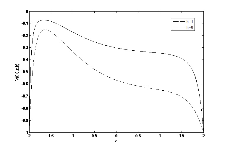
(a) 1

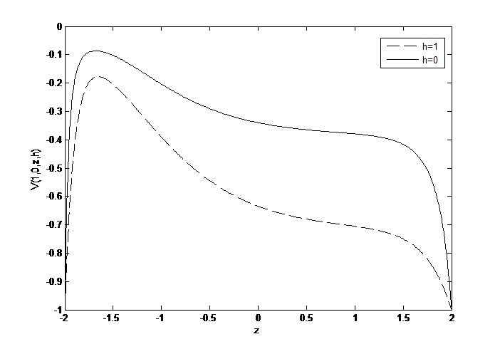
(b) 2

Figure 1.

Observation 3.8.

From FIGURE 1, we conclude the following:

• Assessing model is progressively decreasing by time $t$.

• Assessing procession is progressively increasing by $y$, which can be claimed by the function.

• Before-defaulting assessing model is better than after-defaulting one obviously, which proves that Insurance companies can obtain much more profits after investing surplus in defaultable bonds.

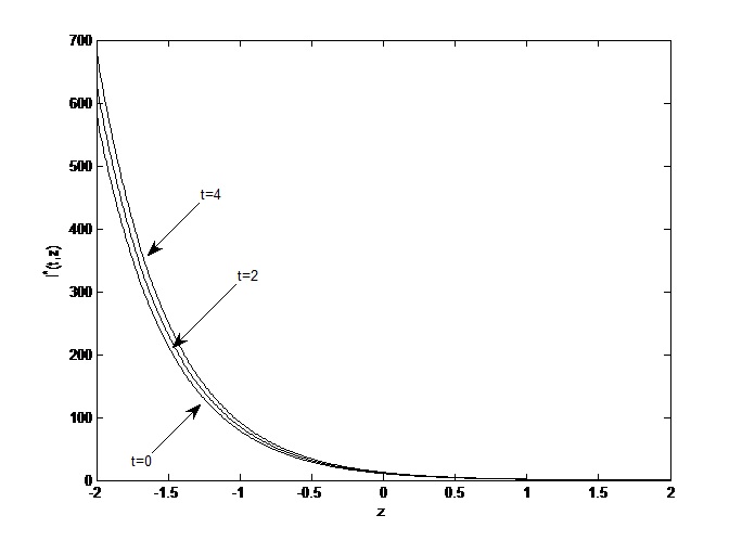
(a) 1

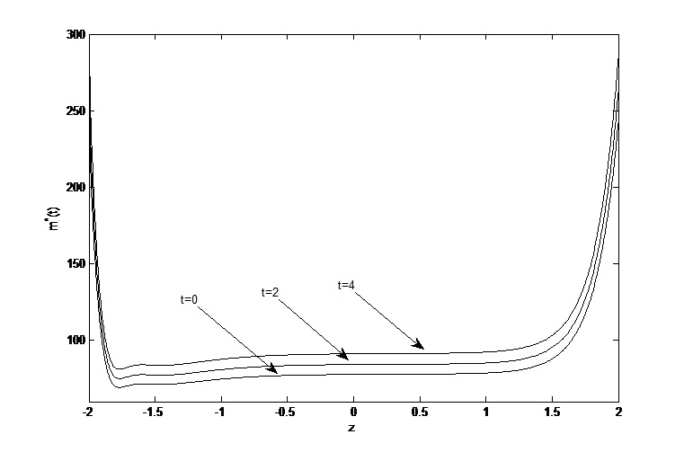
(b) 2

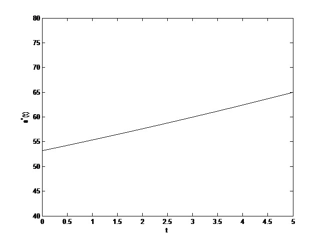
(c) 3

Figure 2.

Observation 3.9.

The tendency of the optimal investing strategies $\pi^{*}(t)=(l^{*}(t),m^{*}(t),a^{*}(t))$ can be presented by FIGURE 2 respectively and the conclusions are followed:

• The investments in the asset of risk market is progressively decreasing in $z$ and increasing in $t$.

• The investments in corporate bond is increasing in $t$. These will drop at first and then increase in $z$.

• The amount of retention of excess-of-loss reinsurance is increasing about $t$.

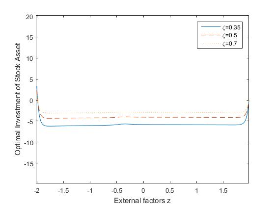
(a) 1

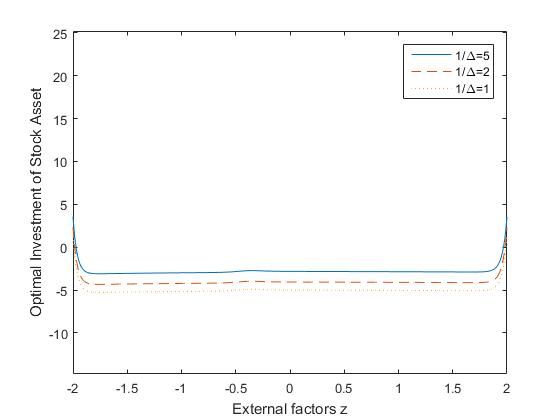
(b) 2

Figure 3. The influence of the external factors of the optimal investment of stock asset with different loss rate and the default premium

Observation 3.10.

Considering the change of interval $\zeta$ and default risk premium $\frac{1}{\Delta}$, we need to make deeper numerical analysis.

• In FIGURE 3(a)1, the external factor leads to the decrease of the optimal strategy at first and then the increase. At the same time, the corporate bond is positively correlated with default risk premium $\frac{1}{\Delta}$. Insurance companies should invest a larger proportion of asset on corporate bond with higher risk of default.

• In FIGURE 3(b)2, the insurer companies will introduce fewer investment in corporate bond when the loss rate is lower. In a nutshell, the adding $\zeta$ reflects few influence on the optimal investment of a corporate bond.

Example 3.11.

Suppose:

$$r=0.04,\mu=0.3,\sigma(z)=e^{z},\delta=0.1,\kappa=1,\lambda=3,\alpha=0.2,\beta=0.3,b=2,d=2,$$

$$T=50,\mu_{\infty}=1/2,\eta=7/3,\theta=8/3,h^{p}=0.25,\Delta=0.25,\zeta=0.4,N=401,M=50001.$$

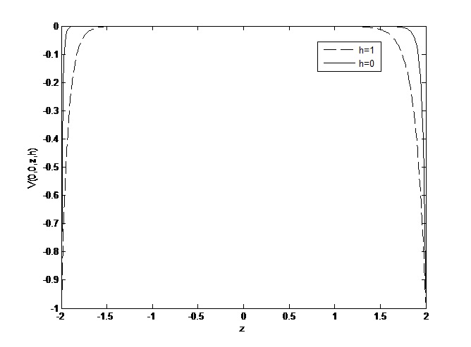
(a) 1

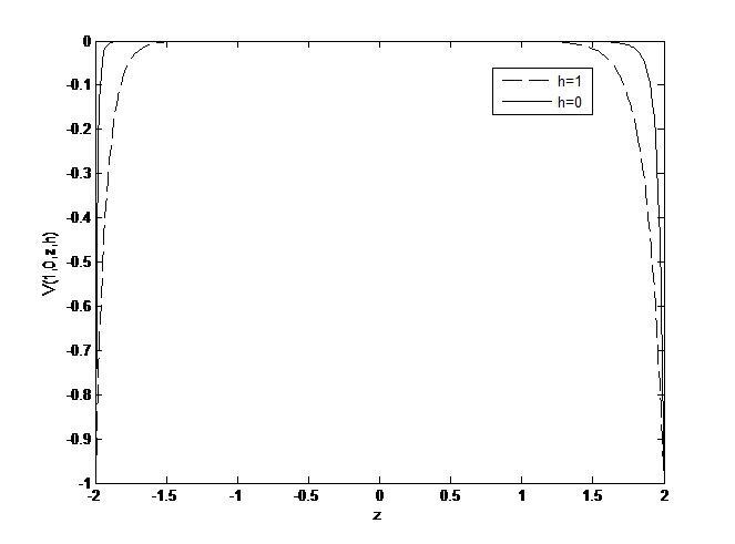
(b) 2

Figure 4.

Observation 3.12.

The FIGURE 4 express the situation of before default and after default. In pictures, the insurance companies can put most money on defaultable cooperate bond for more profit.

Example 3.13.

(The Sensitivity of the Optimal Investment of a Corporate Bond) Assume $T-t=1$, $\alpha=0.5$, $r=0.04$. Then we operate the optimal strategy for $\frac{1}{\Delta}\in[1,10]$ and $\theta\in[0.1,1]$. Firstly, fixing varying parameter $\xi$, we make comparisons between different $\zeta$ and $1/\Delta$. The function of the corporate bond can be expressed as follow:

$$m^{*}(t)=\frac{ln\frac{1}{\Delta}}{\alpha\zeta}.$$ (3.62)

The comparisons were presented by following FIGURE 5.

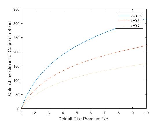
(a) 1

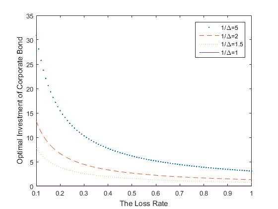
(b) 2

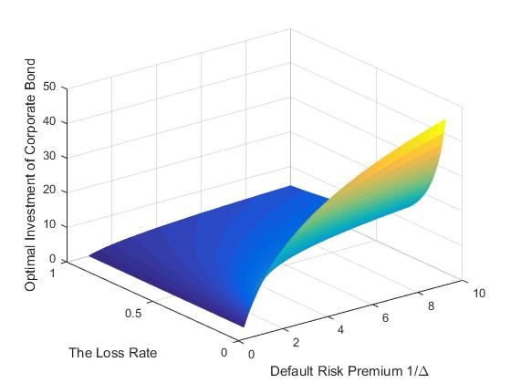
(c) 3

Figure 5. The influence of the loss rate and the default risk premium on the optimal investment of a corporate bond

Observation 3.14.

Herein, we calculate the sensitivity of the optimal investment of a corporate bond. From FIGURE 5 we can tell:

• The optimal investment of corporate for the default risk has positive relationship with default risk premium in FIGURE 5(a)1. The insurance companies will invest a relatively amount of money in a corporate bond with higher default risk condition.

• There is a negative relation between loss rate and the optimal investment in FIGURE 5(b)2. FIGURE 5(b)2 describes that insurer will reduce the investment in corporate bond with increasing loss rate.

• If the risk premium satisfies $\frac{1}{\Delta}=1$, the insurance companies will not invest in corporate bond any more. FIGURE 5(c)3 depicted comprehensive result.

Example 3.15.

(The Effect of RAP on OPRS) When we treat $T=10$, $r=0.04$, the analysis of reinsurance strategy can be explained by exponential value function factor $\alpha$. Now we have $t\in[0,T]$, which means $t\in[0.10]$. We adopted various parameters $\alpha$ in order to compare the effectiveness of optimal excess-of-loss reinsurance. Now the optimal excess-of-loss reinsurance was expressed:

$$\alpha^{*}(t)=\frac{ln(1+\theta)}{\alpha}e^{-r(T-t)}.$$ (3.63)

According to the preconditions, the results can be told by FIGURE 6

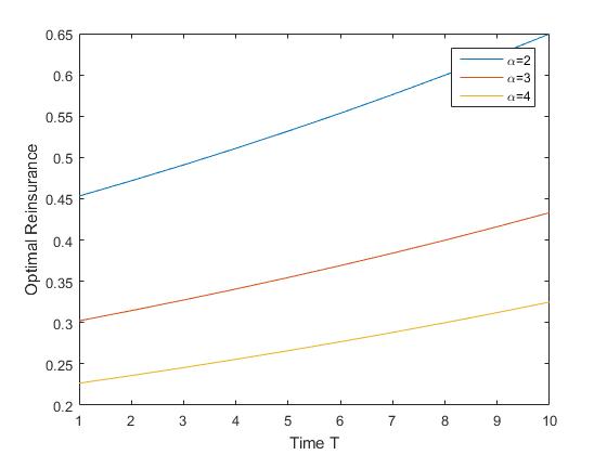
(a) 1

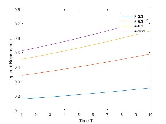
(b) 2

Figure 6. The influence of the insurer’s RAP on OPR

Observation 3.16.

According to FIGURE 6, the conclusions are presented below:

• From FIGURE 6(a)1, The utility of optimal excess reinsurance is increasing in time $t$.

• When the parameter $\alpha$ grows progressively, the effect of the optimal investment is limited. The insurers will be willing to purchase more excess-of-loss reinsurance in order to reduce the risk of investing a value function with higher interval.

• We can compare the safety loading $sigma$. Varying safety loading $sigma$ can generate multiple effects of reinsurance strategies, which can be compared by using previous data.

• From FIGURE 6(b)2, when $sigma$ is bigger, the utility of excess-of-loss reinsurance strategies will be larger. If the insurers purchase the investing products with higher parameter $sigma$, they will need to restrain this kind of investment. In contrast, the companies should invest more money on a strategy with lower $sigma$.

Example 3.17.

(The Effect of RAP on OPRS) The aim of discussion is the relationship between property and exponential value function factor $\alpha$. Suppose $T=10$, $r=0.04$, and then $t\in[0,T]$, which means $t\in[0.10]$.The relation of property $l^{*}(t)$ is:

$$l^{*}(t)=\frac{\mu(z)-r}{\alpha\sigma^{2}(z)}e^{-r(T-t)}.$$ (3.64)

In this function, the volatility $\sigma(z)$ is

$$\sigma(z)=e^{z},z_{i}=-a+(i-1)h,h=\frac{2a}{n-1}.$$ (3.65)

From these functions, we can make further assumption $a=2$ and $n=10$, and then the results are shown as FIGURE 7:

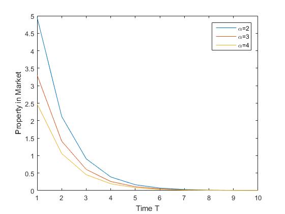
(a) 1

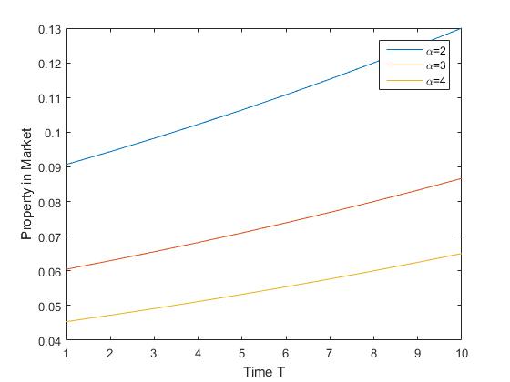
(b) 2

Figure 7. The influence of the insurer’s RAP on OPR

Observation 3.18.

According to FIGURE 7, the conclusions are as follows:

• the longer length of time will result in less utility of investments in market. When the parameter is increasing, the property in investment will reduce. Consequently, for insurers, the investment in large factor $\alpha$ will bring about restricted fortune in risky market.

• If we ignore the volatility of the market or treat all volatility are the same, the result are as what our FIGURE 7(b)2 about. The results are totally different between the result which have same volatility or not.

• Now more and more money are invested in market with increasing time. Obviously, if adding the consideration of volatility, the insurers will put less property on market in longer time. As a result, the longer time will generate lager volatility, larger uncertain factors and larger risk. In order to obtain steady income, we do not need to invest more money on market later. However, when the factor $\alpha$ increases, the money which put on market will reduce. If insurers decide to focus on an investment in value function with a lager parameter, the market property will reduce.

4. Acknowledgments

The authors would like to thank Professor Lijun Bo, for his detailed guidance and instructive suggestions. N. Yao was supported by Natural Science Foundation of China (11101313, 113713283).

5. Appendix

Theorem 5.1.

(Friedman,1975). We consider the following Cauchy problem

$$\left\{\begin{aligned} &u_{t}(x,t)+\mathcal{L}u(x,t)=f(x,t)\quad in\quad\mathbb{R}^{n}\times[0,T)\\ &u(x,T)=h(x)\quad in\quad\mathbb{R}^{n},\end{aligned}\right.$$ (5.1)

Where $\mathcal{L}$ is given by:

$$\mathcal{L}u=\frac{1}{2}\sum_{i,j=1}^{n}a_{ij}(x,t)u_{x_{i}x_{j}}+\sum_{i=1}^{n}b_{i}(x,t)u_{x_{i}}+c(x,t)u.$$

If the Cauchy problem (5.1) satisfies the following conditions:

• The coefficients of $\mathcal{L}$ are uniformly elliptic;

• The functions $a_{ij}$, $b_{i}$ are bounded in $\mathbb{R}^{n}\times[0,T]$ and uniformly Lipschitz continuous in $(x,t)$ in compact subsets of $\mathbb{R}^{n}\times[0,T]$;

• The functions $a_{ij}$ are H$\ddot{o}$lder continuous in $x$, uniformly with respect to $(x,t)$ in $\mathbb{R}^{n}\times[0,T]$;

• The function $c(x,t)$ is bounded in $\mathbb{R}^{n}\times[0,T]$ and uniformly H$\ddot{o}$lder continuous in $(x,t)$ in compact subsets of $\mathbb{R}^{n}\times[0,T]$;

• $f(x,t)$ is continuous in $\mathbb{R}^{n}\times[0,T]$, uniformly H$\ddot{o}$lder continuous in $x$ with respect to $(x,t)$ and $|f(x,t)|\leq B(1+|x|^{\gamma})$;

• $h(x)$ is continuous in $\mathbb{R}^{n}$ and $|h(x)|\leq B(1+|x|^{\gamma})$, with $\gamma>0$;

then there exists a unique solution $u$ of the Cauchy problem (4.1) satisfying:

$$|u(x,t)|\leq const(1+|x|^{\gamma})\quad\quad and\quad\quad|u_{x}(x,t)|\leq const(1+|x|^{\gamma}).$$

Remark 5.2.

In the original theorem of Friedman(1975), the Cauchy problem is given by

$$\left\{\begin{aligned} &v_{t}(x,t)-\mathcal{L}v(x,t)=f(x,t)\quad in\quad\mathbb{R}^{n}\times[0,T)\\ &v(x,0)=h(x)\quad in\quad\mathbb{R}^{n},\end{aligned}\right.$$ (5.2)

We let $v(x,T-t)=u(x,t)$ , then we can get the Cauchy problem shown in (5.1).

References

- [1] Asmussen, S., Hojgaard, B., Taksar, M., Optimal risk control and dividend distribution policies: example of excess–of–loss reinsurance for an insurance corporation[J]. Finance and Stochastics, 2000, 4: 299-324.
- [2] Badaoui, M., Fernández, B., An optimal investment strategy with maximal risk aversion and its ruin probability in the presence of stochastic volatility on investment[J]. Insurance: Mathematics and Economics, 2013 ,53: 1–13.
- [3] Bai, L.H., Guo, J.Y., Optimal proportional reinsurance and investment with multiple risky assets and no–shorting constraint[J]. Insurance: Mathematics and Economics, 2008, 42: 968–975.
- [4] Bebernes, J.W., and Schmitt, K., Invariant sets and the Hukuhara-Kneser property for systems of parabolic partial differential equations. Rocky Mountain J. Math.,1977, 7, 557-567.
- [5] Bebernes, J.W., and Schmitt, K., On the existence of maximal and minimal solutions for parabolic partial differential equations. Proceedings of AMS.,1979,73, 211-218.
- [6] Bielecki, T.R., Rutkowski, M., Credit Risk: Modeling, Valuation and Hedging[M]. Springer, 2002: 225-227.
- [7] Bielecki T R, Jang I., Portfolio optimization with a defaultable security[J]. Asia-Pacific Financial Markets, 2006, 13(2): 113-127.
- [8] Birge, J.R., Bo, L.J., Capponi, A., Risk Sensitive Asset Management and Cascading Defaults, Revised and Resubmitted to Mathematics of Operations Research, 2016.
- [9] Bo L, Li X, Wang Y, et al. Optimal investment and consumption with default risk: HARA utility[J]. Asia-Pacific Financial Markets, 2013, 20(3): 261-281.
- [10] Bo L, Wang Y, Yang X., An optimal portfolio problem in a defaultable market[J]. Advances in Applied Probability, 2010, 42(3): 689-705.
- [11] Browne, S., Optimal investment policies for a firm with a random risk process: exponential utility and minimizing the probability of ruin[J]. Mathematics of Operations Research, 1995, 20: 937–958.
- [12] Cao, Y.S., Wan, N.Q., Optimal proportional reinsurance and investment based on Hamilton–Jacobi–Bellman equation[J]. Insurance: Mathematics and Economics, 2009, 45, 157–162.
- [13] Capponi A, Figueroa–López J E., Dynamic portfolio optimization with a defaultable security and regime–switching[J]. Mathematical Finance, 2014, 24(2): 207-249.
- [14] Castaneda, N., Hernandez, D., Optimal consumption-investment problems in incomplete markets with stochastic coefficients[J]. SIAM Journal on Control and Optimization, 2005, 44 (4): 1322-1344.
- [15] Christensen J H E, Hansen E, Lando D., Confidence sets for continuous-time rating transition probabilities[J]. Journal of Banking and Finance, 2004, 28(11): 2575-2602.
- [16] Cox, J.C., Ross, S.A., The valuation of options for alternative stochasticprocesses[J]. Journal of Financial Economics, 1976, 3: 145–166.
- [17] Duffie D, Pedersen L H, Singleton K J., Modeling sovereign yield spreads: a case study of Russian debt[J]. The Journal of Finance, 2003, 58(1): 119-159.
- [18] Duffie D, Singleton K J., Credit Risk: Pricing, Measurement, and Management: Pricing, Measurement, and Management[M]. Princeton University Press, 2012.
- [19] Fernández, B., Hernández, D., Meda, A., Saavedra, P., An optimal investment strategy with maximal risk aversion and its ruin probability[J]. Mathematical Methods of Operations Research, 2008, 68: 159–179 .
- [20] Fleming, W.H., Soner, H.M., Controlled Markov Processes and Viscosity Solutions[M]. Springer, Berlin, New York, 1993.
- [21] Fouque, J.-P., Papanicolaou, G., Sircar, K.R., Derivatives in Financial Markets with Stochastic Volatility[M]. Cambridge University Press, 2000.
- [22] Friedman, A., Stochastic Differential Equations and Applications[M]. Academic Press., 1975:139-144.
- [23] Friedman, Avner, Partial Differential Equations of Parabolic Type[M]. 1983.
- [24] Gu, M.D., Yang, Y.P., Li, S.D., Zhang, J.Y., Constant elasticity of variance model for proportional reinsurance and investment strategies[J]. Insurance: Mathematics and Economics, 2010, 46: 580–587.
- [25] Heston, S.L., A closed-form solution for options with stochastic volatility with applications to bond and currency options[J]. Review of Financial Studies, 1993, 6: 327–343.
- [26] Hipp, C., Plum, M., Optimal investment for insurers[J]. Insurance: Mathematics and Economics, 2000, 27 : 215–228.
- [27] Hull, J., White, A., The pricing of options on assets with stochastic volatilities[J]. The Journal of Finance, 1987, 42: 281–300.
- [28] Ikeda, N., Watanabe, S., Stochastic differential equations and diffusion processes[J]. 1989.
- [29] Jiao Y, Pham H., Optimal investment with counterparty risk: a default–density model approach[J]. Finance and Stochastics, 2011, 15(4): 725-753.
- [30] Klebaner,F.C, Introduction to Stochastic Calculus with Applications. Imperial College Press, London, 2005.
- [31] Liu, C.S., Yang, H., Optimal investment for an insurer to minimize its probability of ruin[J]. North American Actuarial Journal, 2004, 8: 11–31.
- [32] Lin, X., Li, Y.F., Optimal reinsurance and investment for a jump diffusion risk process under the CEV model[J]. North American Actuarial Journal, 2004, 15: 417–431.
- [33] Liang, Z.B., Yuen, K.C., Cheung, K.C., Optimal reinsurance–investment problem in a constant elasticity of variance stock market for jump–diffusion risk model[J]. Applied Stochastic Models in Business and Industry, 2012, 28: 585–597.
- [34] Li, Z.F., Zeng, Y., Lai, Y.Z., Optimal time–consistent investment and reinsurance strategies for insurers under Heston’s SV model[J]. Insurance: Mathematics and Economics, 2012, 51: 191–203.
- [35] Pham, H., Optimal stopping of controlled jump diffusion processes: a viscosity solution approach[J]. Journal of Mathematical Systems, Estimations, and Control, 1998, 8 (1): 1-27.
- [36] Promislow, D.S., Young, V.R., Minimizing the probability of ruin when claims follow Brownian motion with drift[J]. North American Actuarial Journal, 2005, 9 : 109–128.
- [37] Rama, C., Peter, T., Financial Modelling with Jump Processes. Chapman and Hall, 2003.
- [38] Stein, E.M., Stein, J.C., Stock price distribution with stochastic volatility: an analytic approach[J]. Review of Financial Studies, 1991, 4: 727–752.
- [39] Yang, H., Zhang, L., Optimal investment for insurer with jump-diffusion risk process[J]. Insurance: Mathematics and Economics, 2005, 37: 615–634.
- [40] Zeng, X.D., Taksar, M., A stochastic volatility model and optimal portfolio selection[J]. Quant. Finance, 2003, 13: 1547-1558.
- [41] Zeng, Y., Li, Z.F., Optimal time-consistent investment and reinsurance policies for mean–variance insurers[J]. Insurance: Mathematics and Economics, 2011, 49: 145–154.
- [42] Zhu, H., Deng, C., Yue, S., et al. Optimal reinsurance and investment problem for an insurer with counterparty risk[J]. Insurance: Mathematics and Economics, 2015, 61: 242-254.
- [43] Zhao, H., Rong, X., Zhao, Y., Optimal excess-of-loss reinsurance and investment problem for an insurer with jump–diffusion risk process under the Heston model[J]. Insurance: Mathematics and Economics, 2013, 53: 504-514.