High-precision stellar limb-darkening in exoplanetary transits

Abstract

Characterization of the atmospheres of transiting exoplanets relies on accurate measurements of the extent of the optically thick area of the planet at multiple wavelengths with a precision $\lesssim$100 parts per million (ppm). Next-generation instruments onboard the James Webb Space Telescope (JWST) are expected to achieve $\sim$10 ppm precision for several tens of targets. A similar precision can be obtained in modeling only if other astrophysical effects, including the stellar limb-darkening, are properly accounted for. In this paper, we explore the limits on precision due to the mathematical formulas currently adopted to approximate the stellar limb-darkening, and due to the use of limb-darkening coefficients obtained either from stellar-atmosphere models or empirically. We recommend the use of a two-coefficient limb-darkening law, named “power-2”, which outperforms other two-coefficient laws adopted in the exoplanet literature in most cases, and particularly for cool stars. Empirical limb-darkening based on two-coefficient formulas can be significantly biased, even if the light-curve residuals are nearly photon-noise limited. We demonstrate an optimal strategy to fitting for the four-coefficient limb-darkening in the visible, using prior information on the exoplanet orbital parameters to break some of the degeneracies that otherwise would prevent the convergence of the fit. Infrared observations taken with the James Webb Space Telescope (JWST) will provide accurate measurements of the exoplanet orbital parameters with unprecedented precision, which can be used as priors to improve the stellar limb-darkening characterization, and therefore the inferred exoplanet parameters, from observations in the visible, such as those taken with Kepler/K2, the JWST, and other past and future instruments.

1 Introduction

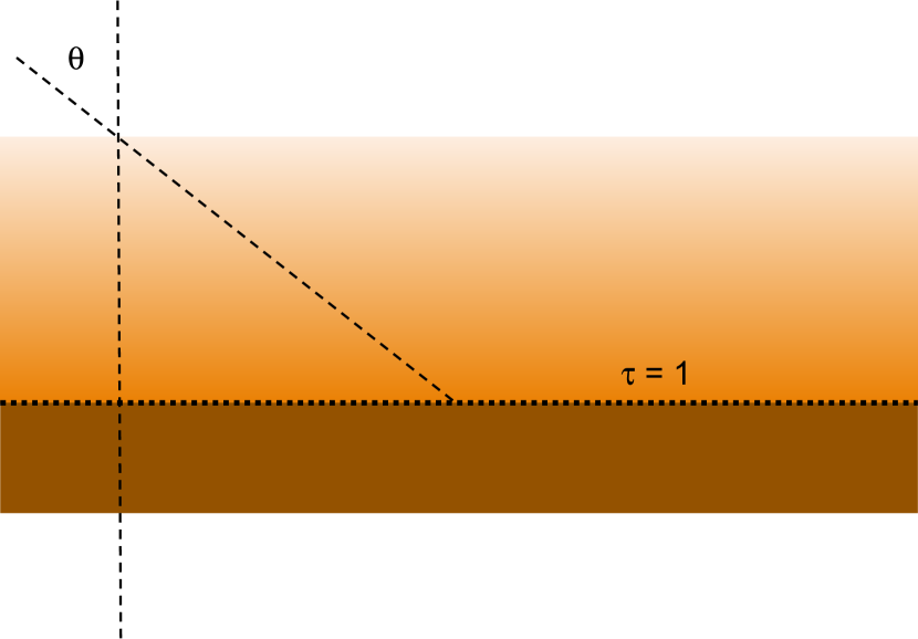
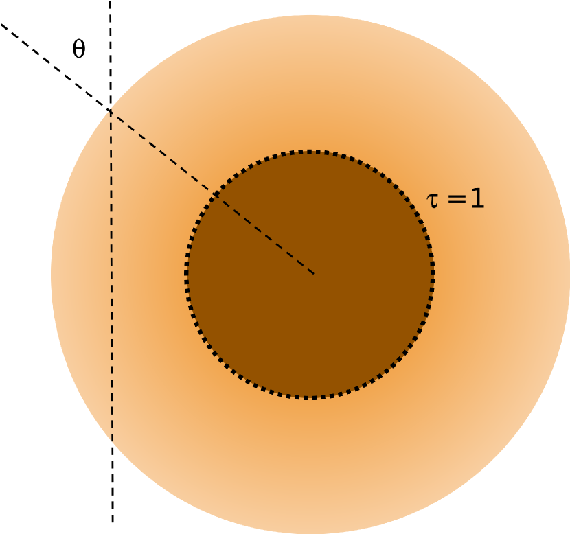
Figure 1: Left panel: illustration of a plane-parallel atmosphere. Right panel: illustration of a spherical-geometry atmosphere (the scale is exaggerated for easier visualization). Note that, differently from the plane-parallel case, the line of sight for the chosen angle $\mu$ does not intersect the shell corresponding to the radial optical depth $\tau=1$.

Observations of transits offer the most accurate means of measuring exoplanet sizes and orbital inclinations, as well as mean stellar densities and, if combined with radial-velocity information, system masses. Transits are revealed through periodic drops in the stellar flux, due to the partial occultation of the stellar disk by the planet for a portion of its orbit. The amplitude of the flux decrement is primarily determined by the size of the planet relative to the star, but also depends on the location of the occulted area of the stellar disk and the wavelength observed, because of limb-darkening (the radial decrease in specific intensity). Inadequate treatment of limb-darkening may give rise to $\gtrsim$10$\%$ errors in exoplanetary radii inferred from transits observed at UV or visible wavelengths, and accurate modeling is paramount in the study of the exoplanetary atmospheres, where differences of 10–100 parts per million (ppm) in transit depths at different wavelengths can be attributed to the wavelength-dependent optical depth of the external layers of the planet, rather than to stellar properties.

Stellar-atmosphere models are commonly used to predict the limb-darkening profiles, but empirical estimates are desirable, both to test the stellar models and to reduce potential biases in transit depths due to errors in the theoretical models or to other second-order effects, such as stellar activity, granulation, gravity darkening, etc.

Other than for the Sun, the surface of which can be directly observed in great detail, techniques to map the stellar intensity distributions rely mainly on optical interferometry (e.g., Hestroffer 1997; Lane et al. 2001; Wittkowski et al. 2001; Aufdenberg et al. 2005) and microlensing (e.g., Witt, 1995; Fields et al., 2003; Dominik, 2004; Zub et al., 2011). The former is useful for only a very limited number of stars with large angular diameters, while the latter is limited by the low occurrence rate and non-repeatability of the microlensing events. Eclipsing binaries offer another route to mapping stellar surfaces, but accurate modeling of these systems is handicapped by complicating factors (gravity darkening, reflection effect, tidal distortion$\ldots$), and a degree of redundancy between limb-darkening and radii. These issues are much reduced in most star+exoplanet systems, thanks to the smaller mass and size of the planetary companions (Wilson & Devinney, 1971; Loeb & Gaudi, 2003; Pfahl et al., 2008).

In this paper, we explore the potential biases in high-precision exoplanet spectroscopy using approximate stellar limb-darkening parameterizations, with coefficients obtained either from stellar-atmosphere models or empirically.

1.1 Structure of the paper

Section 2 reviews the limb-darkening laws most commonly adopted in the exoplanet literature, the proposed power-2 law, and discusses the current approaches to obtain theoretical and empirical limb-darkening coefficients. Section 3 describes how we simulate light-curves from spherical-atmosphere models, and Section 4 reports the results of our analyses. In particular, Section 4.1 outlines the main differences between plane-parallel and spherical stellar-atmosphere models; in Sections 4.2 and 4.3 we analyze the precision with which different limb-darkening laws describe the intensity profile and the transit morphology, and derive the correct transit depth. Section 4.4 describes the equivalent analysis for the case of empirical limb-darkening coefficients, (i.e., allowed as free parameters in the light-curve fit).

Section 4.5 then focuses on the potential errors in ‘narrow-band exoplanet spectroscopy’ over short wavelength ranges, specifically in the context of Hubble Space Telescope (HST)/WFC3 observations. Section 5 examines the ability to fit a set of transit parameters and limb-darkening coefficients on transit light-curves, and develops an optimal strategy to maximize the accuracy in the estimated transit parameters and limb-darkening coefficients in the visible, if infrared observations are also available. Finally, Section 6 discusses the results of our analysis, with emphasis on the synergies between the James Webb Space Telescope (JWST) and Kepler, and on future surveys.

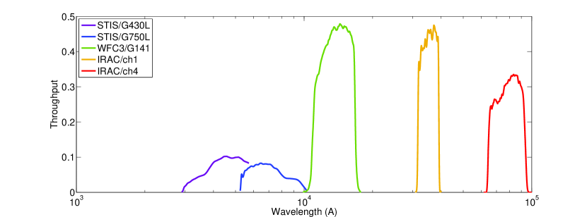
Figure 2: Throughputs of the instruments adopted for the simulations; from visible to mid-infrared, STIS/G430L (purple), STIS/G750L (blue), WFC3/G141 (green), IRAC/ch1 (yellow) and IRAC/ch4 (red).

2 Describing stellar limb-darkening

2.1 Limb-darkening parameterizations

In exoplanetary studies, the stellar limb-darkening profile is typically described by an analytical function $I_{\lambda}(\mu)$, where $I$ denotes the specific intensity, $\mu=\cos{\theta}$, $\theta$ is the angle between the surface normal and the line of sight, and the $\lambda$ subscript refers to the monochromatic wavelength or effective wavelength of the passband at which the specific intensities are given. For circular symmetry, $\mu=\sqrt{1-r^{2}}$, where $r$ is the projected radial co-ordinate normalized to a reference radius.

Numerous functional forms to approximate $I_{\lambda}(\mu)$ have been proposed in the literature. In the study of exoplanetary transits, the most commonly used of these limb-darkening ‘laws’ are:

1. the quadratic law (Kopal, 1950),

   $$\frac{I_{\lambda}(\mu)}{I_{\lambda}(1)}=1-u_{1}(1-\mu)-u_{2}(1-\mu)^{2};$$ (1)

2. the square-root law (Díaz-Cordovés & Giménez, 1992),

   $$\frac{I_{\lambda}(\mu)}{I_{\lambda}(1)}=1-v_{1}(1-\sqrt{\mu})-v_{2}(1-\mu)\text{; and}$$ (2)

3. the four-coefficient law (Claret, 2000),

   $$\frac{I_{\lambda}(\mu)}{I_{\lambda}(1)}=1-\sum_{n=1}^{4}a_{n}\left(1-\mu^{\nicefrac{{n}}{{2}}}\right),$$ (3)

hereinafter referred to as “claret-4”. The quadratic, square-root, and claret-4 laws rely on linear combinations of fixed powers of $\mu$. In this paper, we advocate an alternative two-coefficient law incorporating an arbitrary power of $\mu$ which, to the best of our knowledge, has not previously been considered in the exoplanet literature (and which we initially constructed independently):

1. the ‘power-2’ law (Hestroffer, 1997),

   $$\frac{I_{\lambda}(\mu)}{I_{\lambda}(1)}=1-c\left(1-\mu^{\alpha}\right)$$ (4)

We find that this form offers more flexibility and a better match to model-atmosphere limb-darkening than do other two-coefficient forms (Section 4.2). The claret-4 law can provide a more accurate approximation to model-atmosphere limb-darkening than other forms, but at the expense of using a larger number of coefficients. We note that the quadratic and square-root laws are subsets of the claret-4 prescription, with $a_{1}=a_{3}=0$, $a_{2}=u_{1}+2u_{2}$, $a_{4}=-u_{2}$ (quadratic) and $a_{3}=a_{4}=0$ (square-root). The power-2 form is a subset only for $\alpha=\nicefrac{{1}}{{2}}$, 1, $\nicefrac{{3}}{{2}}$, or 2.

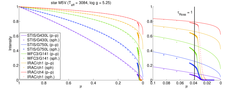
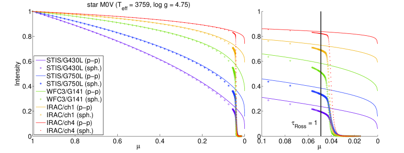
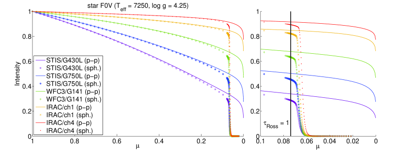
Figure 3: Top to bottom: angular intensity distributions for the M5 V, M0 V, and F0 V models of Table 1. Symbols represent spherical-geometry, passband-integrated intensities for STIS/G430L (purple squares), STIS/G750L (blue “*”), WFC3/G141 (green “+”), IRAC/ch1 (yellow “x”) and IRAC/ch4 (red dots); the corresponding plane-parallel intensities are shown as continuous lines of the same colors. The right-hand panels show the limb region (0.1$\geq\mu\geq$0.0) at a larger scale and the $\mu$ angle corresponding to $\tau_{\mathrm{Ross}}(r)=1$.

2.2 Intensity distributions: plane-parallel vs. spherical

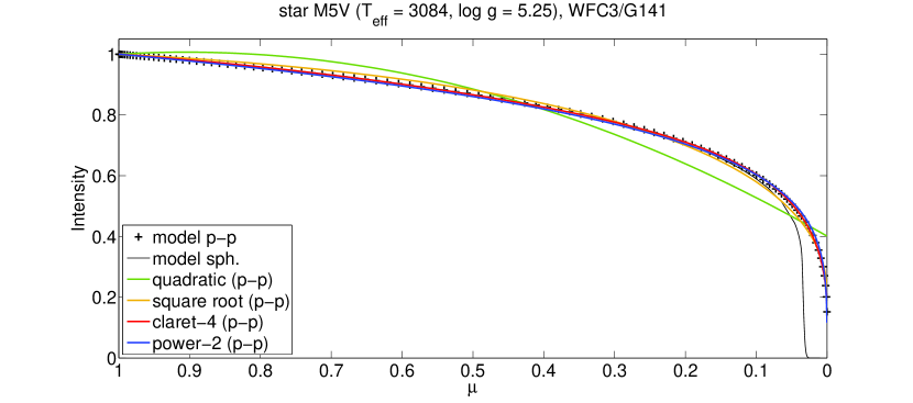
Figure 4: Top panel: Plane-parallel (black “+”) and spherical (black line) model-atmosphere intensities vs. $\mu$ for the M5 V star in the WFC3/G141 passband. Parametric limb-darkening functions fitted to plane-parallel intensities (theoretical models) are quadratic (green), square-root (yellow), claret-4 (red), and power-2 (blue) laws. Bottom panel: large-scale plots of residuals of parametric limb-darkening laws for model-atmosphere intensities in the plane-parallel and spherical geometries (continuous and dashed lines, respectively).

Theoretical limb-darkening coefficients can be obtained from stellar-atmosphere models, by fitting a parametric law (such as Equations 1–4) to detailed numerical evaluations of $I_{\lambda}(\mu)$ using some suitable numerical technique – typically least squares, though detailed numerical results depend on both the method chosen and the data sampling (e.g., Heyrovský, 2007; Claret, 2008; Howarth, 2011). Tables of theoretical limb-darkening coefficients as a function of stellar parameters (usually the effective temperature, gravity, and metallicity) have been published by several authors for various photometric passbands. Most calculations are based on plane-parallel atmosphere models (Claret, 2000, 2004, 2008; Sing, 2010; Howarth, 2011b; Claret et al., 2012, 2013; Reeve & Howarth, 2016), but some authors have considered spherical geometry, claiming, in some cases, noteworthy improvements compared to the use of plane-parallel models (Claret & Bloemen, 2011; Hayek et al., 2012; Neilson & Lester, 2013a, b; Claret et al., 2014; Magic et al., 2015).

These spherical models show a characteristic steep drop-off in intensity at small, but finite $\mu$ (see, e.g., Figure 3). The explanation for this drop-off is straightforward (Figure 1).

In a plane-parallel atmosphere, the optical depth always reaches unity somewhere along the line of sight, even at grazing incidence. The limb of the star is, consequently, geometrically well-defined (and wavelength independent), and the intensity at the limb is comparable to the intensity at the center of the disk, to within a factor of a few.

In spherical geometry, in contrast, there are no constant angles $\mu$ at which the characteristic rays intersect the shells; instead they vary as a function of radius. For technical reasons the emergent intensities are usually specified as functions of the angle as measured at the outer boundary of the model atmosphere, which is originally set by the modeller at an arbitrary physical radius or reference optical depth, subject only to the condition that it has a suitably small opacity and emissivity even at the cores of strong lines. The outermost layer of the model atmosphere, corresponding to $\mu=0$ in this reference frame, is therefore always optically thin and does not correspond to what would be observed as ‘the’ stellar radius in investigations involving interferometric imaging, lunar occultation, or exoplanetary transits. Furthermore, the rapid changes in $I_{\lambda}(\mu)$ that arise at small $\mu$ in spherical models are, inevitably, not well approximated by any of the standard parametric laws developed to represent results of plane-parallel models, because the intensity does not converge to zero at any given radius (see, e.g., Figure 1 of Neilson et al., 2017).

Wittkowski et al. (2004) and Espinoza & Jordan (2015) therefore suggested to re-define $\mu=0$ to a radius outside of which almost no flux is observed, i.e. at the inflection point of the intensity profile so that the tail-like extension originating from the optically thin outer layers is excluded from fitting the limb-darkening profile. The radius is reasonably well defined by the point at which the gradient $dI(\mu)/d\mu$, or almost equivalently $|dI(r)/dr|$, reaches a maximum. Wittkowski et al. (2004) found that this radius corresponded closely to the Rosseland radius, defined by a Rosseland optical depth along the normal $\tau_{\mathrm{Ross}}(r)=1$, for the M giant models they presented. Close to the limb, however, one can expect to observe significant emission as long as the line-of-sight optical depth is at least of order unity. Additionally, in the context of modeling exoplanetary transits, the projected radius for which the total line-of-sight optical depth within the observed wavelength band becomes one should be considered. In Wittkowski et al. (2004) the differences between radial and line-of-sight optical depths at a given physical depth were relatively modest because the giant-star atmosphere they modeled has a large radial extension with corresponding large angles $\mu=0.3$. Furthermore, they studied the emergent intensities in the $K$ band, which has relatively smaller mean opacity than the Rosseland mean, thus partly cancelling the effect of the off-normal incidence.

In this paper, we test empirically the choice of stellar radius, based on the ratios between best-fit and input transit depths (see Section 4.1), finding different values for the best renormalization radius in different wavelength bands (corresponding to the different band-mean opacities). But these radii are larger throughout than the respective $\tau_{\mathrm{Ross}}(r)=1$, which correspond to $\mu=$ 0.0386, 0.049, and 0.0738 for the three models displayed in Figure 3, confirming the effect of the off-normal incidence on the emission near the limb.

2.3 Limitations on empirical limb-darkening coefficients

Empirical limb-darkening coefficients can be inferred by fitting a parametric model to an observed transit light-curve (Mandel & Agol, 2002; Southworth et al., 2004; Pál, 2008) Two-coefficient laws are typically used for this purpose (e.g. Southworth, 2008; Claret, 2009; Kipping & Bakos, 2011, 2011b; Hébrard et al., 2013; Müller et al., 2013), as parameter degeneracies hamper convergence when fitting higher-order models (e.g., the claret-4 characterization).

Measuring empirical limb-darkening coefficients is important to test the validity of the stellar-atmosphere models and, if results are sufficiently accurate, to select the best theoretical models. Furthermore, fixing limb-darkening coefficients at incorrect theoretical values can significantly bias other fitted transit parameters, leading to incorrect inferences about planetary sizes and masses, or confusing the spectral signature of a planetary atmosphere (Csizmadia et al., 2013). In active stars, the presence of dark or bright spots on the surface can change the ‘effective’ limb-darkening coefficients relative to the unperturbed case, as well as the inferred stellar parameters adopted to compute the theoretical coefficients (Ballerini et al., 2012; Csizmadia et al., 2013). Other light-curve distortions may arise from gravity darkening in fast-rotating stars (von Zeipel, 1924; Barnes, 2009; Claret et al., 2012), stellar oscillations (Broomhall et al., 2009; Kjeldsen & Bedding, 2011), granulation (Chiavassa et al., 2016), beaming (Zucker et al., 2007; Shporer et al., 2012), ellipsoidal variations (Pfahl et al., 2008; Welsh et al., 2010), reflected light (Borucki et al., 2009; Snellen et al., 2009), planetary thermal emission (Kipping & Tinetti, 2010), or exomoons (Sartoretti & Schneider, 1999; Kipping, 2009, 2009b). The photometric amplitudes of such distortions can be up to $\sim$100 ppm.

3 Simulated transit light-curves

In order to investigate the consequences of various approximations to limb-darkening, we calculated ‘exact’ synthetic transit photometry as a reference, using new model-atmosphere intensities coupled to an accurate numerical integration scheme for the light-curves.

3.1 Stellar models

We generated three representative model atmospheres using the Phoenix simulator (Allard et al., 2012); input parameters are summarized in Table 1. These models are intended to bracket the range in effective temperature of known exoplanet host stars, and embrace $\sim$98$\%$ of those listed in the exoplanet.eu database (Schneider et al., 2011) as of 2016 December 12.

Table 1: Input parameters (effective temperature, gravity) for solar-abundance Phoenix stellar-atmosphere models adopted for the simulations.

Sp. type	$T_{\rm eff}$	$\log{g}$	$[M/\mbox{H}]$
M5 V	3084	5.25	0.0
M0 V	3759	4.75	0.0
F0 V	7250	4.25	0.0

For each stellar model, $I_{\lambda}(\mu)$ profiles were calculated in both plane-parallel and spherical geometries. In the former case, intensities were calculated at 96 values of $\mu$, chosen as the anchor points for a Gaussian-quadrature integration; the intervals $\Delta\mu_{i}=|\mu_{i+1}-\mu_{i}|$ vary in the range $7\times 10^{-4}$–$1.6\times 10^{-2}$ and are smallest for $\mu\sim$0 and $\sim$1. In spherical geometry, the $\mu$ values were determined by the properties of the model atmosphere, and the number of grid points is model-dependent (169–177 in the cases considered here); the limb is the most finely sampled region, down to $\Delta\mu\sim 6\times 10^{-5}$. Passband-integrated intensities were calculated for five instruments which have been widely used in the field of exoplanet spectroscopy, from the visible to mid-infrared wavelengths: the STIS/G430L, STIS/G750L and WFC3/G141 gratings onboard HST, and the IRAC photometric channels 1 and 4 onboard Spitzer. The throughputs of these instruments are shown in Figure 2, and the corresponding plane-parallel and spherical-model intensities are shown in Figure 3.

3.2 Computing transit light-curves from spherical model atmospheres

We generated two sets of ‘exact’ transit light-curves for the exoplanet-system parameters reported in Table 2. Each set consists of fifteen transit light-curves, one for each stellar model and instrument passband, using the spherical-geometry intensities; the sets differ only in the impact parameter (or, equivalently, the orbital inclination). Each light-curve contains 2001 data points with 8.4 s sampling time, over a $\sim$4.7 hr interval centered on the mid-transit (the total duration of the transits is $\sim$2 hr, with the central transit being $\sim$10 min longer).

Table 2: Input transit parameters adopted in simulations

$p$	$a_{R}$	$i$ (∘)	$e$	$b$	$P$ (days)
0.15	9.0	90.0	0	0.0	2.218573
0.15	9.0	86.81526146	0	0.5	2.218573

The orbital parameters determine $z$, the sky-projected star–planet separation in units of the stellar radius at any given time; for a circular orbit

$$z(t)=a_{R}\sqrt{1-\cos^{2}\left({\frac{2\pi(t-t_{0})}{P}}\right)\sin^{2}(i)},$$ (5)

where $a_{R}$ is the semimajor axis in units of the stellar radius, $P$ is the orbital period, $i$ is the inclination relative to the sky, and $t_{0}$ is the time of conjunction.

The fraction of stellar light occulted by the planet is, for a given intensity profile, a function $F(p,z(t))$, where $p$ is the ratio of planet-to-star radii. Instead of using an analytical function (requiring a numerical approximation to the intensity profile), we computed the light-curve by direct integration of the occulted stellar flux, using our purpose-built ‘tlc’ algorithm. The algorithm:

1. divides the sky-projected stellar disk into a user-defined number of annuli, $n$, with uniform radial separation, $dr=1/n$;

2. evaluates the intensity at the central radius of each annulus, $I(r_{i})$, where $r_{i}=(0.5+i)/n$ for $i=0\dots n-1$, interpolating in $\mu$ from the input stellar-intensity profile (and $r_{i}=\sqrt{1-\mu_{i}^{2}}$);

3. evaluates the flux from each annulus, $F_{i}=I(r_{i})\times 2\pi r_{i}dr$, and hence the total stellar flux, $F_{*}=\sum_{i=0}^{n-1}F_{i}$.

4. The occulted flux is then calculated as $F_{\rm occ}(p,z)=\sum_{i=0}^{n-1}F_{i}f_{z,p}(r_{i})$, where $f_{z,p}(r_{i})$ is the fraction of circumference of each annulus covered by the planet, given by

   $$f_{p,z}(r_{i})=\begin{cases}\frac{1}{\pi}\arccos{\frac{r_{i}^{2}+z^{2}-p^{2}}{2zr_{i}}}&|z-p|<r_{i}<z+p\\ 0&r_{i}\leq z-p\quad\text{or}\quad r_{i}\geq z+p,\\ 1&r_{i}\leq p-z\end{cases}$$ (6)

5. whence the normalized flux is $F(p,z)=1-F_{\rm occ}/F_{*}$.

Before calculating the actual transit light-curves from the spherical model intensities, we tested the accuracy of the algorithm using a wide range of parametric intensity profiles as input, with the same grid of $\mu$ values as the spherical models, comparing the resulting light-curves to those from analytical calculations. We found that, with $n=100\,000$ annuli, the maximum differences between tlc and analytical light-curves were $<5\times 10^{-7}$ in the worst-case scenarios – negligible compared to the minimum uncertainties that can be obtained with any current or forthcoming instrument.

4 modeling transit light-curves

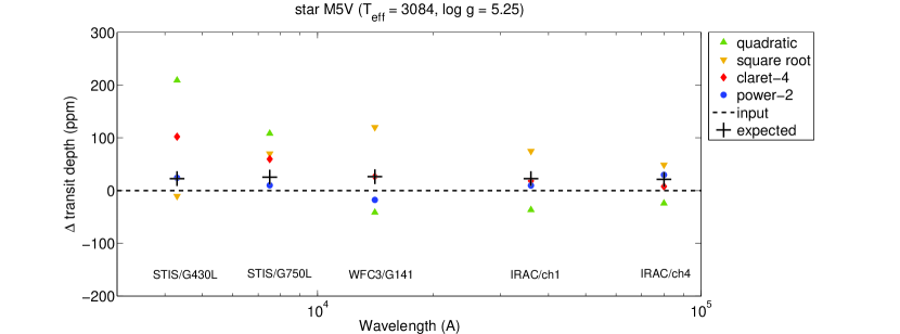
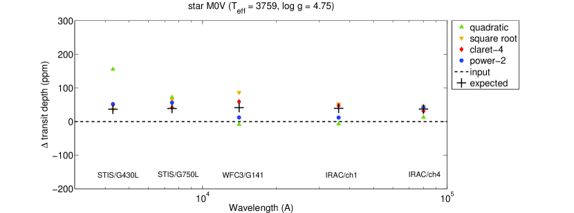
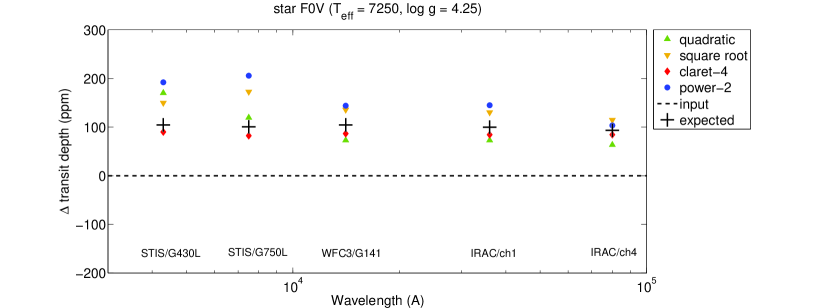
Figure 5: Top panel: differences between the best-fit and the input transit depths for the edge-on transits in front of the M5 V model, using theoretical quadratic (green, upward triangles), square-root (yellow, downward triangles), claret-4 (red diamonds), and power-2 (blue circles) limb-darkening coefficients; the expected values (Equations 7) are indicated with black “+”. Middle, bottom panels: the same for M0 V, and F0 V models.

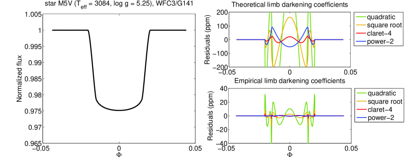
Figure 6: Left panel: exact transit light-curves obtained with $b=0$ for the M5 V star in the WFC3/G141 passband. Right, top panel: residuals for the best-fit transit models using theoretical quadratic (green), square-root (yellow), claret-4 (red), and power-2 (blue) limb-darkening coefficients. Right, bottom panel: residuals obtained with the empirical limb-darkening coefficients.

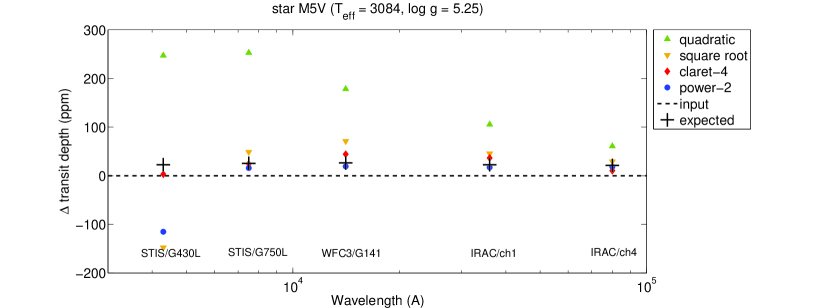
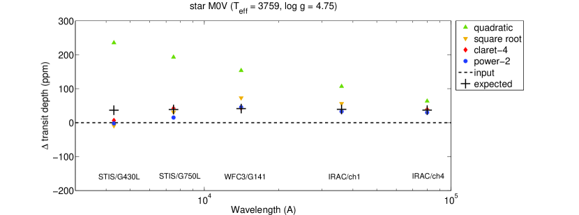
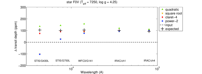
Figure 7: Top panel: differences between the best-fit and the input transit depths for the edge-on transits in front of the M5 V model, using empirical quadratic (green, upward triangles), square-root (yellow, downward triangles), claret-4 (red diamonds), and power-2 (blue circles) limb-darkening coefficients; the expected values (Equations 7) are indicated with black “+”. Middle, bottom panels: the same for M0 V and F0 V models.

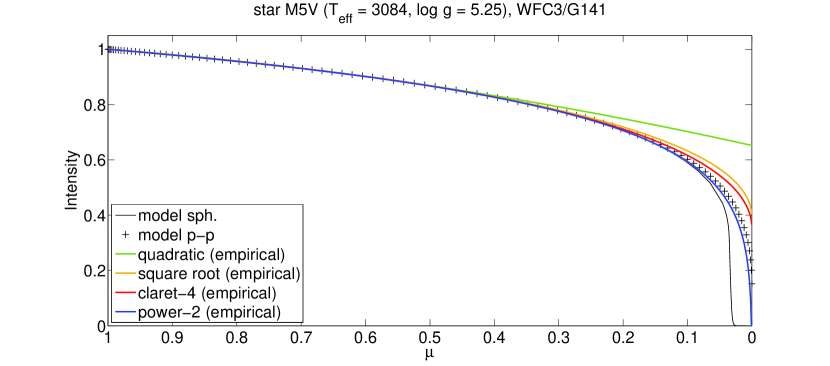
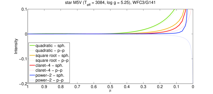
Figure 8: Top panel: Plane-parallel (black “+”) and spherical (black line) model-atmosphere intensities vs. $\mu$ for the M5 V star in the WFC3/G141 passband. Parametric limb-darkening functions inferred from the transit light-curves (empirical models) are quadratic (green), square-root (yellow), claret-4 (red), and power-2 (blue) laws. Bottom panel: large-scale plots of residuals of empirical limb-darkening laws for model-atmosphere intensities in the spherical and plane-parallel geometries (continuous and dashed lines, respectively).

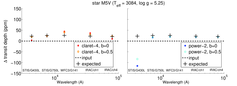
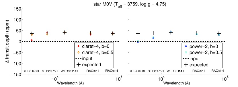
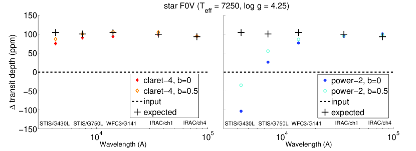
Figure 9: Left panels: differences between the best-fit and input transit depths for the three stellar models, with $b=0$ (red, full diamonds), and 0.5 (orange, empty diamonds), using empirical claret-4 limb-darkening coefficients; the expected values are denoted by black “+”. Right panels: the same, but with empirical power-2 limb-darkening coefficients, $b=0$ (blue, full circles), and 0.5 (cyan, empty circles).

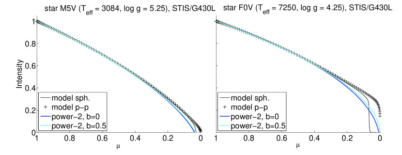
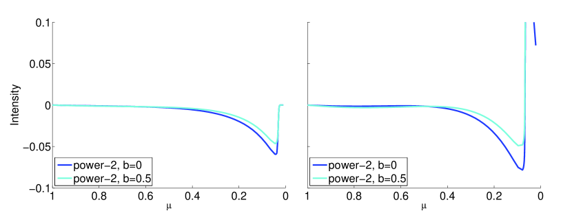
Figure 10: Top, left panel: plane-parallel (black “+”) and spherical (black line) angular intensity vs. $\mu$ for the M5 V model in the STIS/G430L passband; parametric limb-darkening with empirical power-2 coefficients fitted to the transit light-curves with $b=0$ (blue) and 0.5 (cyan). Bottom, left panel: residuals between the parametric models and the spherical intensities. Right panels: the same for the F0 V model in the STIS/G430L passband.

In empirical studies, it is generally convenient to analyse observed transit light-curves using parameterized models in order to fit for the unknown transit parameters and/or limb-darkening coefficients. To mimic this observational approach we employed pylightcurve, our pipeline dedicated to the fast computation of model transit light-curves with a parametric limb-darkening profile. The power-2 parameterization (Equation 4) was implemented in the code for this work. Based on our proposal, the power-2 law has been implemented also in the batman code (Kreidberg, 2015).

4.1 Plane-parallel vs. spherical limb-darkening models

As outlined in Section 2.2, discrepancies between the plane-parallel and spherical limb-darkening models are larger at smaller $\mu$ (i.e., closer to the stellar limb), solely because of the manner in which $\mu$ is defined, at least in the first step, for the spherical models. The spherical models present a steep drop-off in the normalized intensity $I(\mu)/I(1)$, approaching zero at some $\mu>$0, while for the plane-parallel models the intensity is significantly greater than zero for all $\mu$ (see Figure 3).

It is reasonable to suppose that the ‘photometric’ stellar radius relevant to transit studies is better represented by the projected radius of the intensity drop-off than by $\mu=0$, the arbitrary uppermost layer in the atmospheric model. As a pragmatic approach, we assign this projected photometric radius to the point in the intensity distribution at which the gradient $\text{d}I(\mu)/{\text{d}}\mu$ reaches a maximum (estimated as the mean $\mu$ value between the two consecutive $\mu$ values in the model with the maximum difference quotient, $|I(\mu_{i+1})-I(\mu_{i})|/|\mu_{i+1}-\mu_{i}|$). The corresponding radius, $r_{0}=\sqrt{1-\mu_{0}^{2}}$, hereinafter called the ‘apparent’ radius, is the ratio between the stellar photometric radius and the radius of the outermost layer in the model. Our approach is similar to what is suggested by Wittkowski et al. (2004) and Espinoza & Jordan (2015), but here we compute the photometric radius for each passband, while they calculate one wavelength-averaged photometric radius.

With this working definition, the best-fit model parameters for any of our simulated transit light-curves are expected to deviate from their input values according to:

$$p_{\rm expected}^{2} \simeq\left(\frac{p_{\rm input}}{r_{0}}\right)^{2}$$ (7)

$$a_{R,{\rm expected}} \simeq\frac{a_{R,{\rm input}}}{r_{0}}$$ (8)

$$i_{\rm expected} \simeq i_{\rm input}.$$ (9)

Table 3 reports the ranges of $r_{0}$ over the five instrument passbands for the given stellar model, the corresponding percentage variation in transit depth, $p^{2}=(R_{p}/R_{*})^{2}$, and the absolute variation evaluated at $p_{\rm input}=0.15$.

Table 3: Measured ranges of apparent stellar radius, $r_{0}$, over five instrument passbands for the three stellar models; corresponding percentage variations in transit depth, $p^{2}=(R_{p}/R_{*})^{2}$; and absolute variations, evaluated at $p_{\rm input}=0.15$.

Sp. type	$r_{0}$ range	$\frac{p_{\rm exp}^{2}-p_{\rm input}^{2}}{p_{\rm input}^{2}}$	$p_{\rm exp}^{2}-p_{\rm input}^{2}$
($T_{\rm eff}$, $\log{g}$)			$|_{p=0.15}$
M5 V,	0.99942–0.99953	0.09–0.12$\%$	21–26 ppm
(3084, 5.25)
M0 V,	0.99908–0.99919	0.16–0.18$\%$	37–41 ppm
(3759, 4.75)
F0 V,	0.99769–0.99794	0.41–0.46$\%$	93–104 ppm
(7250, 4.25)

In the analytical approximations represented by Equations 7–8, we find the apparent stellar radius to be systematically smaller than the radius of the uppermost layer of these models by 0.05–0.1$\%$ for the M dwarfs, and up to $\sim$0.2$\%$ for the F0-star model; the corresponding percentage errors in transit depths are about twice as large. For the case of a transiting hot Jupiter ($p=0.15$), the discrepancies in transit depth are at the level of $\sim$20, 40, and 100 ppm for the two M dwarfs and for the F0 model, respectively. The discrepancies measured for the F0 model currently represent practical upper limits for exoplanet host stars, given that $\sim$99% of the current population is cooler, and hence have less extended atmospheres (for given $\log{g}$). The wavelength-dependence of the apparent radius is negligible over the parameter space explored here, with a peak-to-peak amplitude of 11 ppm, in transit depth, from visible to mid-infrared wavelengths in the worst-case scenario (see Table 3).

4.2 Accuracy of the theoretical limb-darkening laws

We fitted the limb-darkening laws to the plane-parallel intensity profiles by adopting a simple least-squares method in the fits. We checked, both by using subsets of the precalculated intensity grids and interpolating at different angles, that similar results would be obtained using a uniform sampling in $\mu$. Figure 4 shows the corresponding best-fit models, hereinafter referred as “theoretical” limb-darkening models, and their residuals, for the case of the M5 V observed in the WFC3 passband. The full list of models and the relevant residuals are reported in Figure 22 (Appendix A). The power-2 law (Equation 4) outperforms the other two-coefficient laws at describing the stellar limb-darkening of all stars observed at near to mid-infrared wavelengths with the HST/WFC3 and Spitzer/IRAC instruments; in some cases, the power-2 model outperforms even the corresponding claret-4 one. At visible wavelengths, the square-root and power-2 models have comparable success, while the claret-4 models fit best. The average errors in specific intensity predicted by the power-2 models are in the range 0.1–1.0%, with a maximum error up to $\sim$5–7% for the F0 V model in the visible passbands. The claret-4 models are more uniformly robust among all the configurations, with average errors in the range 0.05–0.6% and maximum errors $<$4%. The quadratic models are the least accurate of those tested, with average errors in the range 1–6% and maximum errors of up to 25% (for the M0 V model in the WFC3 passband).

4.3 Transit models with theoretical limb-darkening coefficients

We measured the potential biases in the model transit depths by fixing the limb-darkening coefficients at the theoretical values obtained from the plane-parallel stellar-atmosphere models and fitting the exact light-curves described in Section 3.2. The free parameters in the fit were $p$, the ratio of planet-to-star radii, $a_{R}$, the orbital semimajor axis in units of the stellar radius, and $i$, the orbital inclination. We used a Nelder–Mead minimization algorithm to find the values of these parameters which minimize the residuals between the model fits and the exact light-curves. We then carried out Markov-chain Monte-Carlo (MCMC) runs with 300,000 iterations to assess the robustness of the point estimates. Unlike previous investigations reported in the literature (e.g. Csizmadia et al., 2013), we seek to isolate the potential biases arising from the analysis method, and particularly the use of simplified geometry and a parameterization to characterize the stellar limb-darkening. No other astrophysical sources of error are considered in this study.

Figure 5 illustrates the differences between the best-fit transit depths and input values for $i=90^{\circ}$; the expected values (from Equations 7–8) are also indicated. For all stellar models, the results are less dependent on the parametric law at longer wavelengths; this is to be expected, since the limb-darkening is smaller at longer wavelengths. In particular, the transit depths obtained at 8$\mu$m (IRAC channel 4) are all within 45 ppm of expected values, or within 13 ppm if adopting the power-2 or claret-4 coefficients. Overall, the transit depths obtained using the claret-4 coefficients deviate by less than $\sim$20 ppm from expected values, other than for the M5 V model in the visible passbands, where the discrepancy reaches 34 and 80 ppm for the STIS/G750L and STIS/G430L passbands. The peak-to-peak amplitudes in best-fit transit depths over the five passbands are 94, 28, and 8 ppm, going from the coolest to the hottest model. The results obtained with the power-2 coefficients are more robust for the cooler stars, and are within 44 ppm of expected values, except for the F0 V model in the visible passbands, where the inferred transit depths are 105 and 88 ppm larger for the STIS/G750L and STIS/G430L passbands. The peak-to-peak amplitudes in best-fit transit depths over the five passbands are 47, 44, and 102 ppm, again from the coolest to the hottest model. The quadratic-law coefficients have the largest scatter in the best-fit transit depth across the different passbands for all models, with peak-to-peak amplitudes of 250, 164, and 107 ppm.

Even though the true value of the transit depth is not known in a ‘real-world’ scenario, the presence of biases can be revealed by time-correlated noise in the light-curve residuals. Figure 6 shows the residuals between the exact light-curve and the best-fit parametric model for the M5 V star in the WFC3 passband. The full list of light-curve residuals is reported in Figure 23. The amplitudes of the time-correlated residuals (maximum discrepancies from zero) are in the ranges 97–456, 8–105, and 11–75 ppm with quadratic, power-2, and claret-4 models respectively. Residuals at infrared wavelengths are typically smaller than in the visible, as expected. Neilson et al. (2017) report similar amplitudes for the residuals between the exact light-curves, computed with their CLIV stellar-atmosphere models, and parametric light-curve models. For comparison, residuals with $\sim$10 ppm root mean square (rms) amplitude have been obtained from the phase-folded Kepler photometry of several targets (e.g., Barnes et al., 2011; Müller et al., 2013), and $\sim$50–200 ppm rms amplitude is typically obtained for the white light-curves observed with the HST/WFC3 (e.g., Deming et al., 2013; Tsiaras et al., 2016, 2016b).

It is possible that better results would be obtained if the limb-darkening coefficients were fitted adopting a different sampling in $\mu$ (e.g., uniform in $r$ rather than in $\mu$), a different method (e.g., imposing flux-conservation), and/or using spherical intensities (e.g., Sing, 2010; Claret & Bloemen, 2011; Howarth, 2011; Espinoza & Jordan, 2015). A detailed study of the different approaches is beyond the scope of this paper, but the analysis in Section 4.4 provides some clear indications.

4.4 Transit models with empirical limb-darkening coefficients

4.4.1 Edge-on transits

We repeated the fits to the exact light-curves with the limb-darkening coefficients as free parameters (in addition to $p$, $a_{R}$, and $i$). The increased flexibility allows parametric models that better match the transits, as shown by the smaller time-correlated residuals in Figures 6 and 23 (Appendix A). The residual amplitudes are in the range 10–63, 0–31, and 0–4 ppm with quadratic, power-2, and claret-4 models respectively. The time-correlated residuals due to imperfections in the transit models with empirical limb-darkening coefficients are hardly detectable with current instruments.

Figure 7 shows the corresponding best-fit transit depths. Despite the very small light-curve residuals, the inferred transit depth can be significantly biased. The bias obtained with quadratic limb-darkening is roughly linear in the logarithm of wavelength for the two M dwarfs, ranging from 27–40 ppm at 8$\mu$m to 200–225 ppm at 0.4$\mu$m; there is no evident trend for the F0 V model, but the transit depth is again systematically over-estimated, by 17–52 ppm. The square-root and power-2 laws have similar performances, with deviations from the expected values smaller than 45 ppm, except for three ‘bad’ points: the STIS/G430L passband for the M5 V model, and the STIS/G430L and STIS/G750L passbands for the F0 V model, for which the transit depth estimates are smaller than the apparent values by 170–138, 207–205, and 74–73 ppm for the two laws. The transit depth estimates obtained when fitting the claret-4 coefficients are the most accurate, with deviations from the expected values being smaller than 30 ppm (largest in the STIS/G430L passband) and peak-to-peak amplitudes of 41, 36, and 24 ppm from the coolest to the hottest model.

Figure 8 shows the empirical limb-darkening models and their residuals for the case of the M5 V observed in the WFC3 passband. The full list of models and the relevant residuals are reported in Figure 24 (Appendix A). It appears that the empirical limb-darkening models are better constrained at larger $\mu$ values, corresponding to the inner part of the disk. We also found that the empirical coefficients can be obtained from the stellar-atmosphere models if a uniform sampling in $r$ rather than in $\mu$ is used. However, if a functional form is not able to reproduce the intensity profile, the empirical model will be particularly discrepant at the limb, causing larger biases in the best-fit transit depth compared to the case of theoretical coefficients with a uniform sampling in $\mu$. Quadratic models, especially, always overpredict the intensities at the limb, so that an apparently larger planet would be needed to occult the extra stellar flux, in agreement with the larger transit depth estimates.

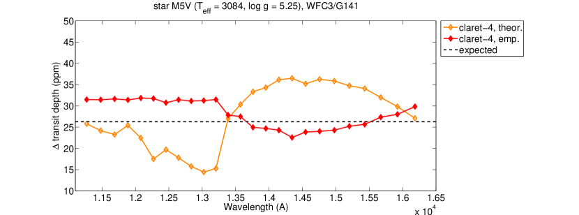
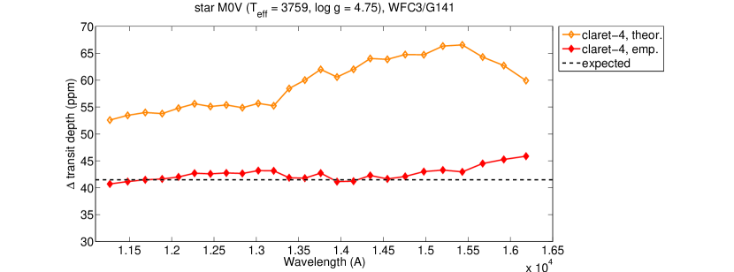
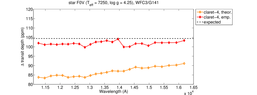
Figure 11: Top panel: differences between the best-fit and the input transit depths for the M5 V model over twenty-five wavelength bins in the WFC3/G141 passband, with $b=0$, using theoretical (orange, empty diamonds) and empirical (red, full diamonds) claret-4 coefficients.

4.4.2 Inclined transits

For randomly orientated orbits, the inclinations $i$ are distributed such that the probability density of $\cos{i}$ is uniform between 0 and 1. For circular orbits, therefore, the impact parameter, $b=a_{R}\cos{i}$, is uniformly distributed between 0 and $a_{R}$, the semimajor axis in units of stellar radius. An exoplanet transits if and only if $0\leq b<1+p$. We tested the ability to constrain the stellar limb-darkening profile and to measure the correct transit depth changes for the case $b=0.5$. This study was conducted for the claret-4 and power-2 laws, as they led to more robust results than the other parameterizations. In this configuration, the area of the stellar disk with $r<b-p=0.35$, or $\mu\gtrsim 0.94$, is never occulted by the transiting exoplanet.

Figure 9 shows the comparison between the transit depths estimated for the cases with $b=0$ and 0.5, using the claret-4 and power-2 laws. In most cases, there are no significant differences in transit depth obtained for the cases with $b=0$ and 0.5. The largest discrepancies (29–68 ppm) are registered for the three ‘bad’ points of the power-2 law, which are highlighted in Section 4.4.1. The empirical limb-darkening profiles are also very similar. Figure 10 shows the difference for the two most discrepant cases. The parametric models obtained from the transits with $b=0.5$ approximate the intensities at the limb slightly better than those obtained from the transits with $b=0$, but the bias is also significant. In general, it appears that, if a parametric law does not allow a good approximation of the limb-darkening profile, the empirical model is optimized toward the center of the disk and significantly deviates at the limb (see also the quadratic fits in Figure 8). In these cases, inclined transits automatically attribute slightly higher weights to the intensities at the limb, as the planet spends more time occulting areas further from the center. Even if the innermost region of the stellar disk is not sampled during the transit, this is not often a problem, at least if $b\lesssim 0.5$, because the intensity gradient does not vary significantly near the center. The examples discussed here may suggest that inclined transits can lead to smaller biases in the inferred transit parameters and limb-darkening profiles than edge-on transits, but the improvements appear to be quite small and, more importantly, the error bars have not yet been considered.

4.5 Narrow-band (WFC3-like) exoplanet spectroscopy

The results discussed in Section 4.4.1 may suggest that it is difficult to model the depth of a hot-Jupiter transit with an absolute precision better than $\sim$10–30 ppm, because of the intrinsic limitations of the stellar limb-darkening parameterizations (claret-4 being the most accurate among those currently used). This potential bias will be particularly important when analyzing visible to mid-infrared exoplanet spectra measured with the JWST, as it is comparable with the instrumental precision limit (Beichman et al., 2014).

In this section, we investigate the potential errors in relative transit depth over multiple narrow bands within a limited wavelength range, so-called “narrow-band exoplanet spectroscopy”. This kind of measurement has been performed with HST/STIS (Charbonneau et al., 2002; Vidal-Madjar et al., 2003, 2004), Spitzer/IRS (Grillmair et al., 2007, 2008; Richardson et al., 2007), HST/NICMOS (Swain et al., 2008, 2009, 2009b; Tinetti et al., 2010), HST/WFC3 (Deming et al., 2013; Crouzet et al., 2014; Fraine et al., 2014; Knutson et al., 2014, 2014b; Kreidberg et al., 2014, 2014b, 2015; McCullough et al., 2014; Stevenson et al., 2014; Line et al., 2016; Tsiaras et al., 2016, 2016b), and other space- and ground-based spectrographs (e.g. Redfield et al., 2008; Snellen et al., 2008; Swain et al., 2010; Danielski et al., 2014), leading to the discovery of a long list of atomic, ionic, and molecular species in the atmospheres of exoplanets.

Since the detection of the chemical species relies on their spectral features, it is not affected by a constant offset in transit depth; hence only the errors in transit depth differences at multiple wavelengths, referred to as relative error, are important. Here, we study the case of exoplanet spectroscopy with HST/WFC3, for which the narrow-band spectra reported in the literature often have $\sim$20–40 ppm error bars.

To fix the ideas, we considered 25 wavelength bins, identical to those ones adopted in Tsiaras et al. (2016b), to generate one set of exact light-curves (as in Section 3.2) for each stellar model, and calculate the theoretical limb-darkening coefficients. We modeled each exact light-curve using the two approaches outlined in Sections 4.3 and 4.4, i.e., with the theoretical and empirical limb-darkening coefficients, respectively.

Figure 11 shows the spectra obtained by using the most accurate claret-4 law. The spectra calculated with the theoretical limb-darkening coefficients are offset by $+1$, $+18$, and $-18$ ppm, on average, in excellent agreement with the measured biases for the broadband light-curves reported in Section 4.3. The relative errors, as measured by the peak-to-peak amplitudes, are 22, 14, and 8 ppm, from the coolest to the hottest model. The use of empirical limb-darkening coefficients reduces the spectral offsets, in these cases, to less than 3 ppm, and also reduces the peak-to-peak amplitudes down to 9, 5, and 4 ppm, respectively. Note that, in all configurations, the peak-to-peak amplitudes across the WFC3 narrow bands are smaller than the respective amplitudes for the broadband photometry from visible to mid-infrared reported in Section 4.3 and 4.4, and they also decrease with the increasing model temperature.

We remind the reader that the results discussed up to this section focus on the potential biases due to the approximate stellar limb-darkening parameterizations, in the absence of noise. The limits of the actual parameter fitting for light-curves with a low, but realistic, noise level are discussed in Section 5. An additional complication is the presence of temporal gaps in the transit light-curves observed with instruments onboard the HST, and from satellites operating on low orbits in general. The impact of such gaps in the retrieval of the transit parameters will be discussed in a separate paper (Karpouzas et al. 2017, in preparation).

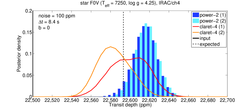
Figure 12: MCMC-sampled posterior distributions of modeled transit depth for the edge-on transit, F0 V model, IRAC/ch4 passband, with 100 ppm gaussian noise (fitting $p$, $a_{R}$, $i$, normalization factor, and limb-darkening coefficients). The histogram channels (blue and light-blue) are for two chains with 1 500 000 iterations, using the power-2 law; the channels are half-thick and shifted to improve their visualization. The red and orange lines denote the analogous posterior distributions when using the claret-4 law. The input and expected transit depths are also indicated (black vertical lines, continuous and dashed, respectively).

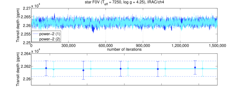
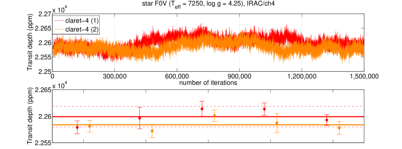
Figure 13: Top panels: transit depth chains for the edge-on transit, F0 V model, IRAC/ch4 passband, with 100 ppm gaussian noise, fitting $p$, $a_{R}$, $i$, normalization factor, and power-2 (blue and light-blue) or claret-4 (red and orange) limb-darkening coefficients. Bottom panels: mean values and standard deviations calculated over fractional chains with 300 000 iterations; the horizontal lines indicate the mean values calculated over the full chains (continuous lines), and the mean values plus or minus the standard deviations (dashed lines).

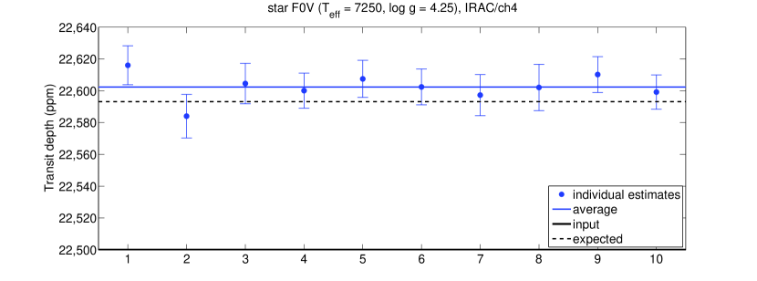
Figure 14: Transit depth estimates for the edge-on transit in front of the F0 V model, IRAC/ch4 passband, with 100 ppm gaussian noise (different noise time series, blue); fitting $p$, $a_{R}$, $i$, normalization factor, and power-2 limb-darkening coefficients. Average over the ten light-curves (blue, continuous line), input (black, continuous line) and expected (black, dashed line) values.

5 Light-curve fitting with empirical limb-darkening coefficients

Sections 4.3 and 4.4 discussed the intrinsic biases due to the use of parametric models with theoretical (plane-parallel) or empirical limb-darkening coefficients. We now consider fitting the transit models with empirical limb-darkening coefficients to more realistic light-curves with noise. Those light-curves are obtained by adding gaussian time series to the exact light-curves (see Section 3.2). The standard deviation for the noise time series was set at $\sim$100 ppm, which is similar to the best photon-noise limit possible for a short-cadence Kepler frame (Van Cleve & Caldwell, 2009), or for a single HST/WFC3 scan (Deming et al., 2013; Tsiaras et al., 2016b), taking into account the different integration times. We focused on four cases: two transits with $b=0$ and 0.5 across the hottest model star, at 8 $\mu$m (F0 V model, IRAC/ch4 passband), and across the coolest model star, at $\sim$430 nm (M5 V model, STIS/G430L passband). The cases considered correspond to those for which the limb-darkening effects are weakest (mid-infrared) and strongest (visible).

5.1 F0 V model, IRAC/ch4 passband

Figure 12 shows the transit depth posterior distributions for the $b=0$ transit and F0 V model in the IRAC/ch4 passband, MCMC sampled with 1 500 000 iterations. Figure 13 reports the relevant chains. Similar parameter chains are computed, in parallel, for $a_{R}$, $i$, the limb-darkening coefficients, a normalization factor, and the likelihood’s variance. In two cases, the limb-darkening coefficients for the power-2 law are fitted, in the other two cases the claret-4 ones. The sampled posterior distributions of the transit depth, using the power-2 limb-darkening law, are almost identical and, in particular, the mean values and standard deviations differ by less than 1 ppm. Even considering subsets of the chains with 300 000 samples, the mean values and standard deviations are stable to better than 5 ppm. It may appear from Figure 12 that the results are biased, given that the peak of the posterior distribution is more than 1$\sigma$ away from the expected value. However, by repeating the analysis with different noise realizations, the best-fit transit depth is within 1$\sigma$ of the expected value in 7 cases out of 10, consistent with the expectations for gaussian noise (see Figure 14). Interestingly, the average of the individual best-fit transit depths is 9 ppm above the expected value, which is very close to the 7 ppm bias measured in the noiseless case (Section 4.4). The chains calculated with the claret-4 law present significant long-term modulations, resulting in wider posterior distributions; there are also moderately large differences between the two repetitions, indicating that they have not converged. The lack of convergence when fitting the claret-4 coefficients is not a surprise, and it is due to strong correlations between the coefficients and with the other transit parameters.

Figures 25 and 26 (Appendix B) show the posterior distribution and chains obtained for the inclined transit, with $b=0.5$, using the power-2 limb-darkening law. The posterior distributions are wider than those obtained for the edge-on transit, with $1\sigma\approx 20$ ppm rather than 12 ppm. The estimates from the partial chains with 300 000 samples are also less robust, with the corresponding mean values scattered over a 12 ppm interval.

The accuracy and precision of the empirical limb-darkening profiles are discussed in Appendix C.

5.2 M5 V model, STIS/G430L passband

We conducted corresponding studies for two transits in front of the M5 V model in the STIS/G430L passband. Figure 15 shows the transit depth posterior distributions for the edge-on transit, and Figure 16 reports the relevant chains. The sampled posterior distributions of the transit depth, using the power-2 limb-darkening law, are in good agreement and, in particular, the mean values differ by 10 ppm, with standard deviations of 45 and 48 ppm, respectively. As expected, the error bars are larger than those obtained for the less limb-darkened case (with identical noise). The estimates from the fractional chains with 300 000 samples may differ by up to 35 ppm, and the relevant standard deviations are in the range 34–51 ppm. Even in this case, the MCMC process failed to converge when fitting the claret-4 coefficients. Figure 17 reports the transit depth estimates obtained with 10 different noise realizations, using the power-2 law. Note that their average is significantly biased in the same direction as the bias obtained in absence of noise (see Section 4.4), and the 1-$\sigma$ error bars are smaller than the bias.

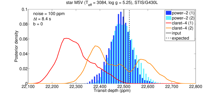
Figure 15: MCMC-sampled posterior distributions of modeled transit depth for the edge-on transit, M5 V model, STIS/G430L passband, with 100 ppm gaussian noise (fitting $p$, $a_{R}$, $i$, normalization factor, and limb-darkening coefficients). The histogram channels (blue and light-blue) are for two chains with 1 500 000 iterations, using the power-2 law; the channels are half-thick and shifted to improve their visualization. The red and orange lines denote the analogous posterior distributions when using the claret-4 law. The input and expected transit depths are also indicated (black vertical lines, continuous and dashed, respectively).

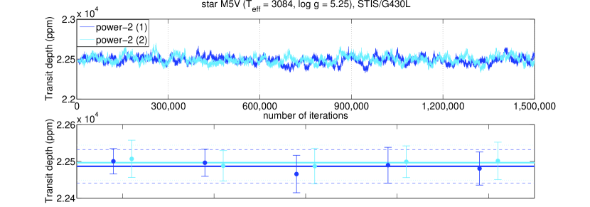
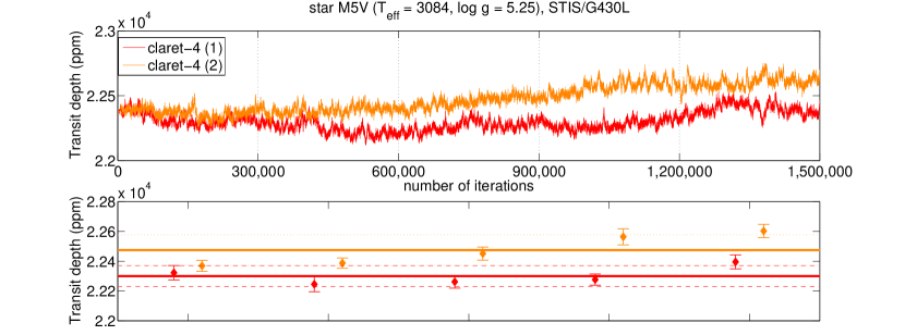
Figure 16: Top panels: transit depth chains for the edge-on transit, M5 V model, STIS/G430L passband, with 100 ppm gaussian noise, fitting $p$, $a_{R}$, $i$, normalization factor and power-2 (blue and light-blue) or claret-4 (red and orange) limb-darkening coefficients. Bottom panels: mean values and standard deviations calculated over fractional chains with 300 000 iterations; the horizontal lines indicate the mean values calculated over the full chains (continuous lines), and the mean values plus or minus the standard deviations (dashed lines).

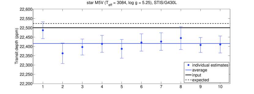
Figure 17: Transit depth estimates for the edge-on transit in front of the M5 V model, STIS/G430L passband, with 100 ppm gaussian noise (different noise time series, blue); fitting $p$, $a_{R}$, $i$, normalization factor, and power-2 limb-darkening coefficients. Average over the ten light-curves (blue, continuous line), input (black, continuous line) and expected (black, dashed line) values.

Figures 27 and 28 (Appendix B) show the posterior distribution and chains obtained for the inclined transit, with $b=0.5$, using the power-2 limb-darkening law. The posterior distributions are wider than those obtained for the edge-on transit, i.e. 1$\sigma\approx$ 115 ppm rather than 45 ppm.

The accuracy and precision of the empirical limb-darkening profiles are discussed in Appendix C.

5.3 The benefits of using prior information

The examples discussed in Section 5.1 and 5.2 show that:

1. if using the power-2 law, the empirical limb-darkening coefficients can be fitted with the other transit parameters ($p$, $a_{R}$, $i$; see Section 3.2) and a normalization factor, but the results can be significantly biased, depending on the stellar model and passband;

2. the analogous fits, using the claret-4 law, fail to converge (at least, using our MCMC routine with up to 1 500 000 iterations).

Unfortunately, all the two-coefficients laws are biased for some stellar types and wavelengths (see Section 4.3 and 4.4), but most of them are sufficiently accurate in the infrared wavelengths. Some authors proposed to fitting one or two coefficients of the claret-4 law, while keeping the other coefficients fixed (e.g., Howarth & Morello, 2017). We found that the validity of this approach relies on a good choice of the fixed coefficients, and thus is not fully empirical.

Our proposal is that, if the ‘geometric’ parameters, $a_{R}$ and $i$, are measured in the infrared, the results can be implemented as an informative prior when fitting at shorter wavelengths, thanks to their small or negligible wavelength-dependence, based on Equations 8, 9 and Table 3. We tested fitting for $p$, $a_{R}$, $i$, the claret-4 limb-darkening coefficients, and a normalization factor, on the transit light-curves obtained for the M5 V model in the STIS/G430L passband, adopting gaussian priors on $a_{R}$ and $i$. The parameters of the gaussian priors are reported in Table 4.

Table 4: Parameters of the gaussian priors adopted in Section 5.3.

	$\mu(a_{R})$	$\sigma(a_{R})$	$\mu(i)$	$\sigma(i)$
$b=0$	9.0042	0.004	90	0.18
$b=0.5$	9.0042	0.006	86.81526146	0.01

Figure 18 shows the transit depth posterior distributions for the edge-on and the inclined transits, obtained with 1 500 000 MCMC samples. Figure 19 shows the relevant chains.

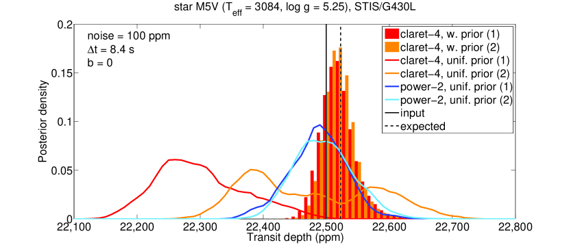
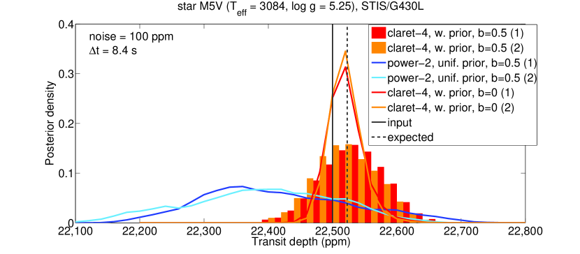
Figure 18: Top panel: MCMC-sampled posterior distributions of modeled transit depth for the edge-on transit in front of the M5 V model, STIS/G430L passband, with 100 ppm gaussian noise; fitting $p$, $a_{R}$, $i$, normalization factor and limb-darkening coefficients. The histogram channels (red and orange) are for two chains with 1 500 000 iterations, using claret-4 coefficients and gaussian priors on $a_{R}$ and $i$; the channels are half-thick and shifted to improve their visualization. Other lines denote the posterior distributions obtained with non-informative priors for all parameters and claret-4 (red and orange) or power-2 (blue and light-blue) limb-darkening coefficients. The input and expected transit depths are also indicated (black vertical lines, continuous and dashed, respectively). Bottom panel: analogous for the inclined transit ($b=0.5$), except the red and orange lines report the histograms from the top panel for comparison.

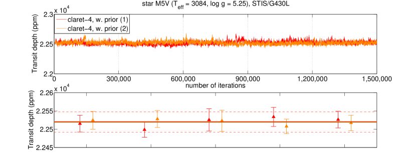
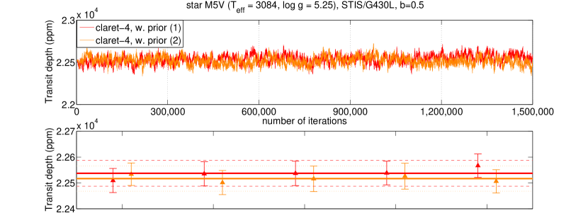
Figure 19: Top panels: transit depth chains for the edge-on transit, M5 V model, STIS/G430L passband, with 100 ppm gaussian noise, fitting $p$, $a_{R}$, $i$, normalization factor and claret-4 limb-darkening coefficients, adopting gaussian priors on $a_{R}$ and $i$. Bottom panels: mean values and standard deviations calculated over fractional chains with 300 000 iterations; the horizontal lines indicate the mean values calculated over the full chains (continuous lines), and the mean values plus or minus the standard deviations (dashed lines).

The use of gaussian priors on $a_{R}$ and $i$ leads to convergence of the MCMC fits with claret-4 coefficients. The error bars in transit depth are significantly smaller than those estimated with power-2 limb-darkening coefficients and non-informative priors on $a_{R}$ and $i$, falling to $\sim$25 and $\sim$50 (compared with $\sim$45 and $\sim$115 ppm), for the edge-on and inclined transits, respectively. The biases, averaged over 10 light-curves with different noise levels, are also smaller (+15 and -7 ppm; Figure 20).

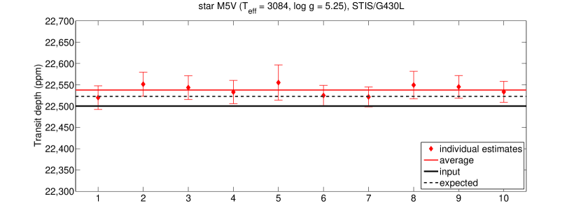
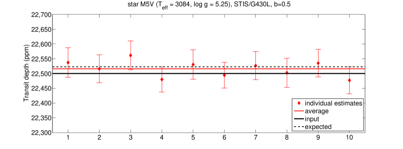
Figure 20: Top panel: transit depth estimates for the edge-on transit in front of the M5 V model, STIS/G430L passband, with 100 ppm gaussian noise (different noise time series, red); fitting $p$, $a_{R}$, $i$, normalization factor and claret-4 limb-darkening coefficients, adopting gaussian priors on $a_{R}$ and $i$. Average over the ten light-curves (red, continuous line), input (black, continuous line) and expected (black, dashed line) values. Bottom panel: the same, for the inclined transit ($b=0.5$).

As a final test, we investigated the effect of having a longer integration time, similar to that of the Kepler short-cadence frame. The longer integration time is simulated by binning the transit light-curves over 7 points ($7\times 8.4=58.8$ s). The relevant transit depth posterior distributions are shown in Figure 21; they are almost identical to the non-binned ones.

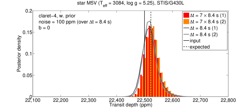
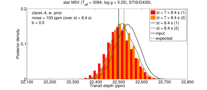
Figure 21: Top panel: MCMC-sampled posterior distributions of modeled transit depth for the edge-on transit in front of the M5 V model, STIS/G430L passband, with 100 ppm gaussian noise, then binned over 7 points; fitting $p$, $a_{R}$, $i$, normalization factor and claret-4 limb-darkening coefficients, adopting gaussian priors on $a_{R}$ and $i$. The histogram channels (red and orange) are for two chains with 1 500 000 iterations, using claret-4 coefficients and gaussian priors on $a_{R}$ and $i$; the channels are half-thick and shifted to improve their visualization. The grey lines denote the analogous posterior distributions without binning. The input and expected transit depths are also indicated (black vertical lines, continuous and dashed, respectively). Bottom panel: the same, for the inclined transit ($b=0.5$).

We conclude that an integration time of $\sim$1 min, as for the Kepler short-cadence frames, does not affect the accuracy (error bar) of the fitted transit depth, compared to shorter integration times.

6 Discussion

6.1 Synergies between JWST and Kepler, K2, TESS

Empirical limb-darkening coefficients determined from exoplanetary transit light-curves are desirable, not only to validate the stellar-atmosphere models, but also to improve both the absolute and relative precision of inferred exoplanetary spectra. No two-coefficient limb-darkening law is accurate for all stellar types and/or wavelengths, but can still give near-perfect fits to the transit light-curves, albeit with significantly biased transit parameters and limb-darkening coefficients. To overcome this issue, fitting for the claret-4 limb-darkening coefficients is necessary, but some prior knowledge of the orbital parameters $a_{R}$ and $i$ is required to enable convergence of the fitting algorithms.

Such knowledge can be obtained from the infrared observations, for which the effect of limb-darkening is smaller, and simple two-coefficient laws may be sufficiently accurate. The MIRI instrument onboard JWST will provide suitable observations for tens of exoplanets. A re-analysis of the Kepler and K2 targets, with the approach developed in Section 5.3, can address some of the controversies reported in the literature (e.g. Southworth, 2008; Claret, 2009; Kipping & Bakos, 2011; Müller et al., 2013), if the only problem was the use of inadequate two-parameter limb-darkening laws. The same approach should be used for new observations that will be obtained, in the visible, by TESS and/or other JWST instruments.

7 Conclusions

We studied the potential biases in transit depth due to the use of theoretical stellar limb-darkening coefficients obtained from plane-parallel model atmospheres, and when fitting for empirical limb-darkening coefficients, over a range of model temperatures and instrumental passbands. We propose the use of a two-coefficient law, named “power-2”, which outperforms the most common two-coefficient laws adopted in the exoplanet literature, especially for the M-dwarf models. Nevertheless, the Claret four-coefficient law is significantly more robust than any simpler one, especially at visible wavelengths. Our results indicate that an absolute precision of $\lesssim$30 ppm can be achieved in the modeled transit depth at visible and infrared wavelegths, with $\lesssim$10 ppm relative precision over the HST/WFC3 passband, depending on the stellar type. The intrinsic bias due to the use of theoretical limb-darkening coefficients obtained from plane-parallel models is also $\lesssim$30 ppm for most exoplanet host stars (F–M spectral types), but this estimate does not take into account the uncertainties in the stellar models and in the measured stellar parameters, or the effect of stellar activity and other second-order effects.

Finally, we developed an optimal strategy to fitting for the four-coefficient limb-darkening in the visible, using prior information on the exoplanet orbital parameters to break some of the degeneracies. This novel approach could solve some of the controversial results reported in the literature, which relies on empirical estimates of quadratic limb-darkening coefficients. The forthcoming JWST mission will provide accurate information on the orbital parameters of transiting exoplanets through observations performed by MIRI, enabling wide application of the approach developed in this paper.

Appendix A Supplemental figures: best-fit models and residuals

This Appendix contains Figures 22–24 showing the best-fit limb-darkening and transit models for each stellar type and passband analyzed in Sections 4.1–4.4.

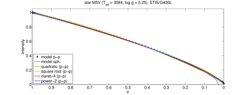
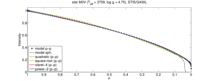
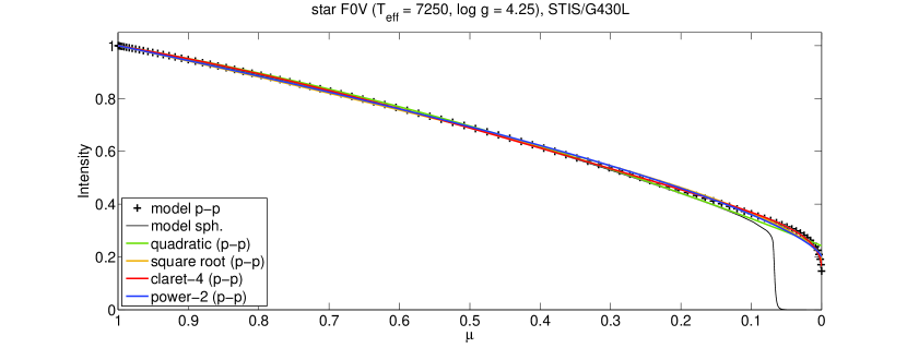
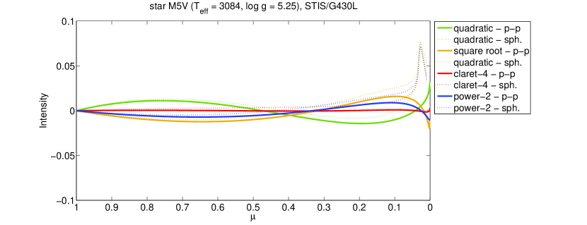
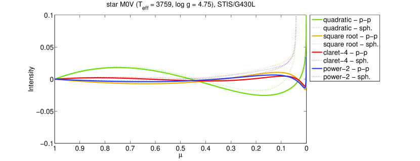
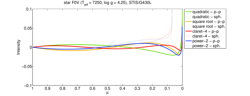
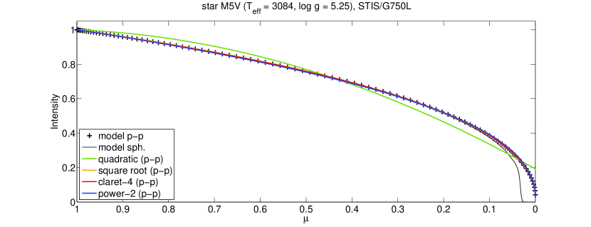
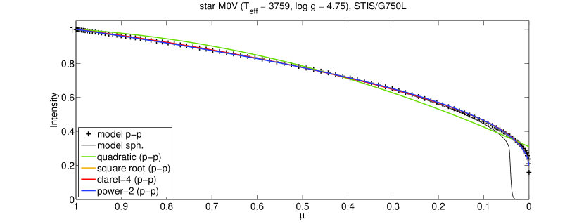
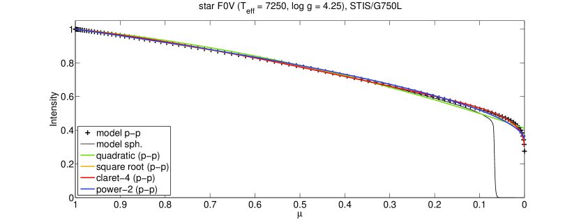
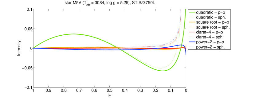
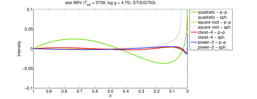
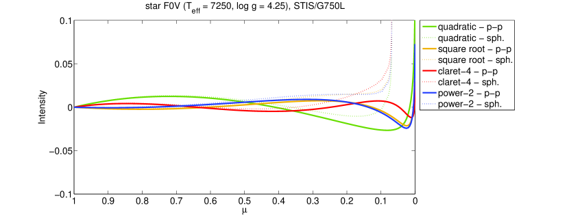
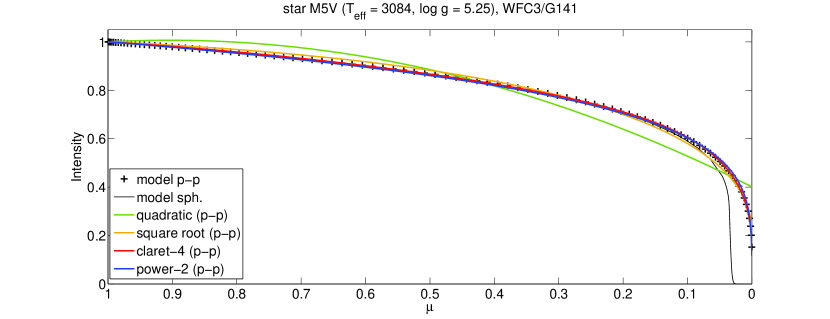
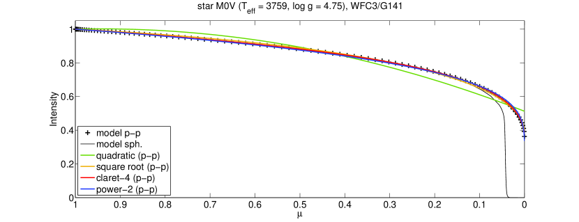
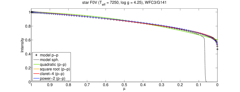
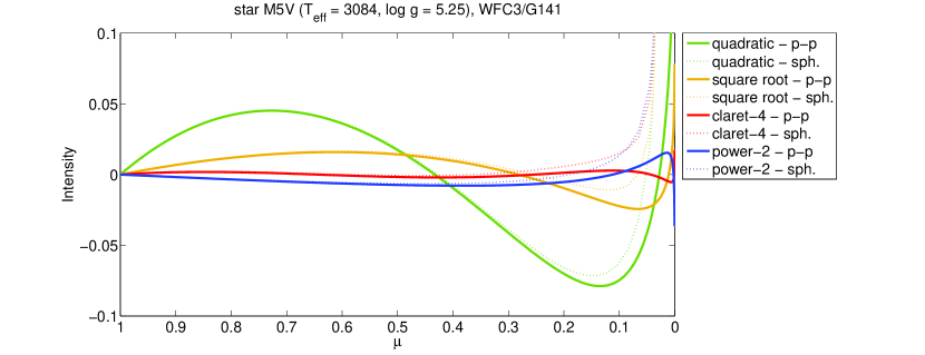
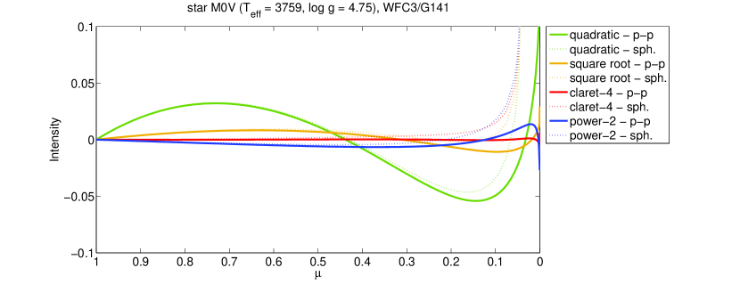
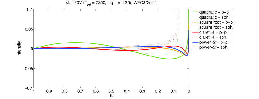
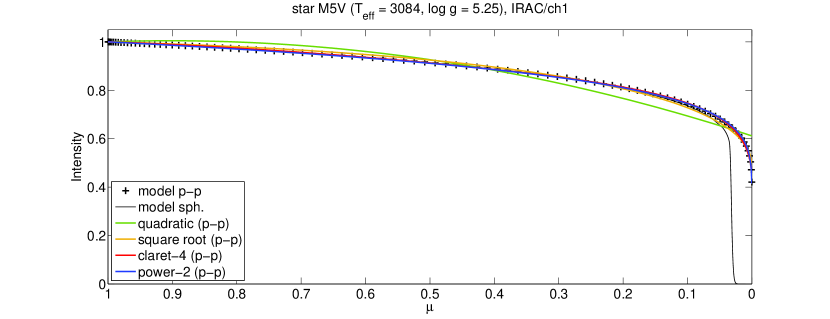
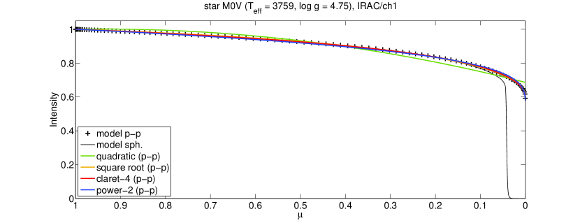
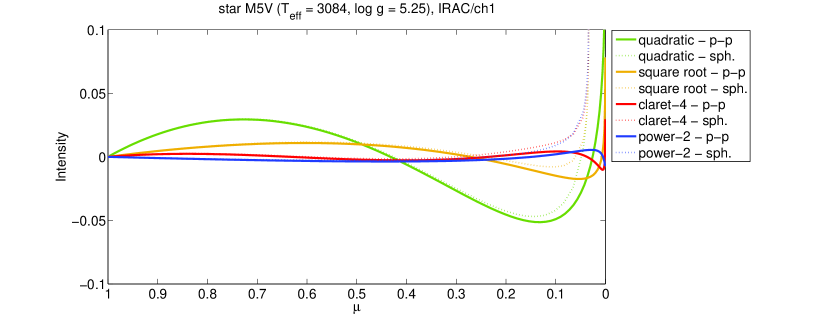
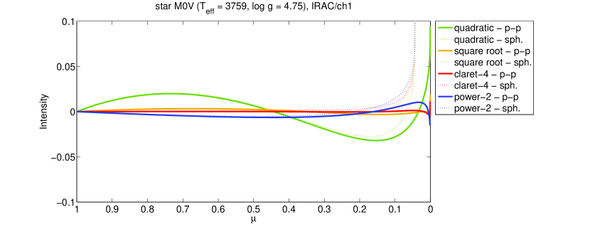
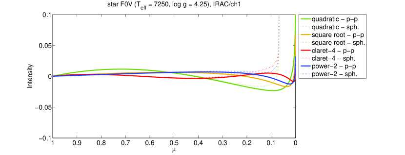
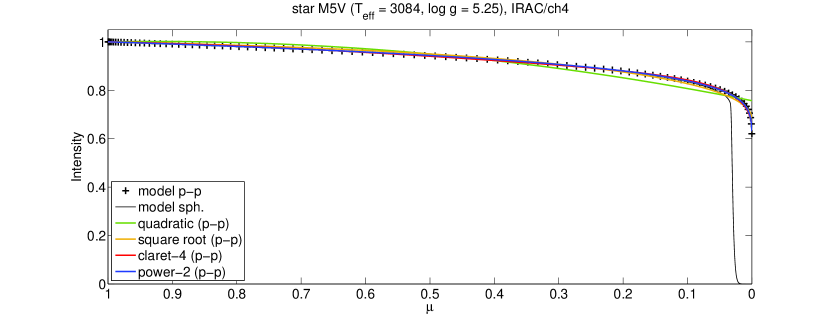
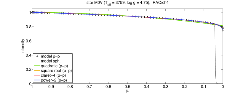
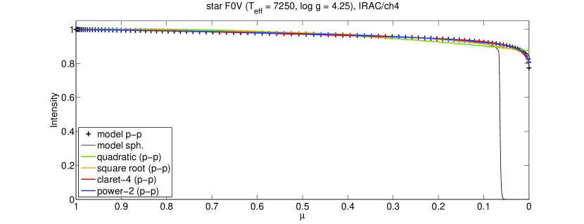
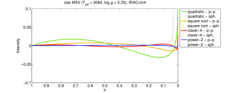
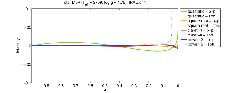
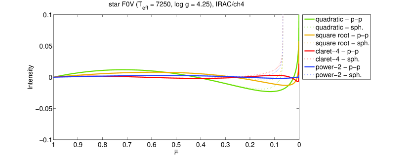
Figure 22: Top panels: Plane-parallel (black ‘+’) and spherical (black line) model-atmosphere intensities vs. $\mu$. Parametric limb- darkening functions fitted to plane-parallel intensities are quadratic (green), square-root (yellow), claret-4 (red), and power-2 (blue) laws.
Bottom panels: large-scale plots of residuals of parametric limb-darkening laws for model-atmosphere intensities in the plane-parallel and spherical geometries (continuos and dashed lines, respectively).

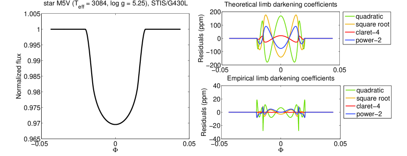
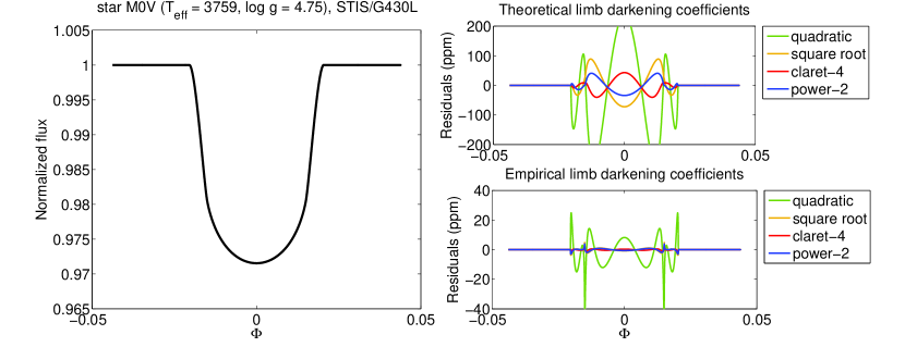
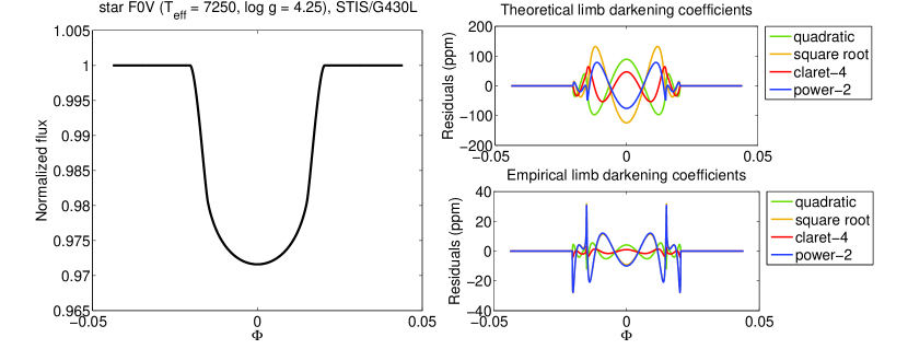
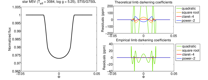
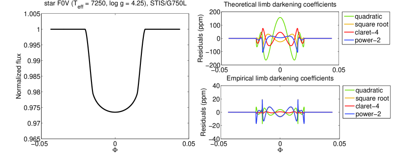
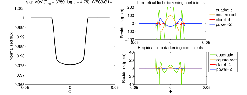
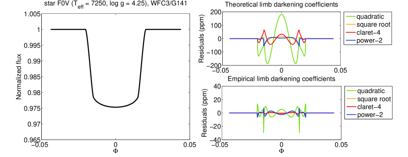
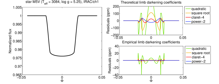
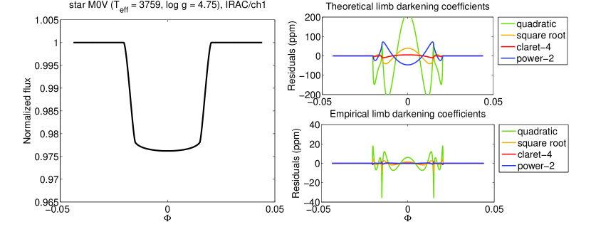
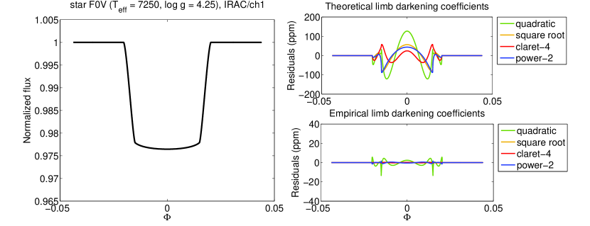
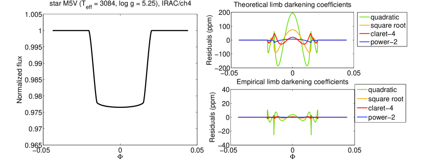
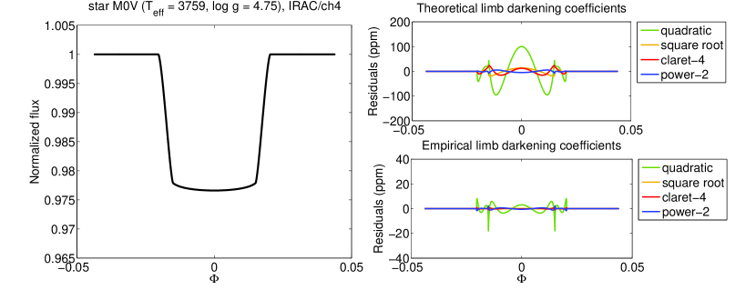
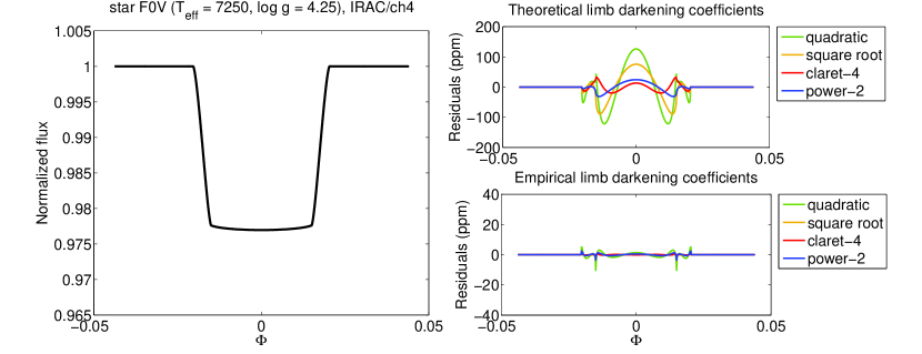
Figure 23: Left panels: exact transit light-curves obtained with $b=0$. Right, top panels: residuals for the best-fit transit models using fixed quadratic (green), square-root (yellow), claret-4 (red), and power-2 (blue) limb-darkening coefficients. The coefficients are fitted to the plane-parallel angular intensities. Right, bottom panels: residuals obtained with the empirical limb-darkening coefficients.

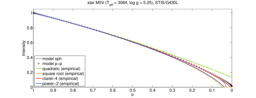
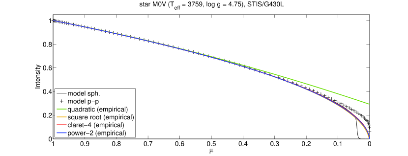
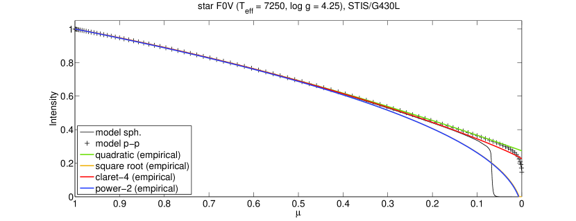
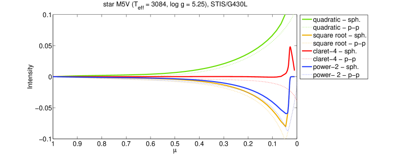
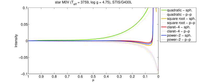
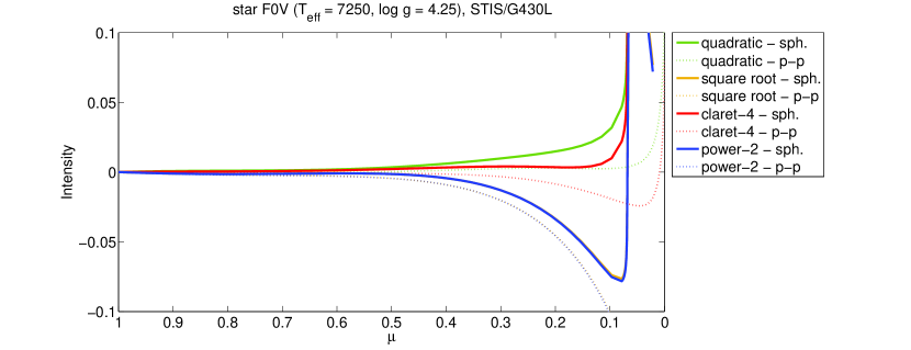
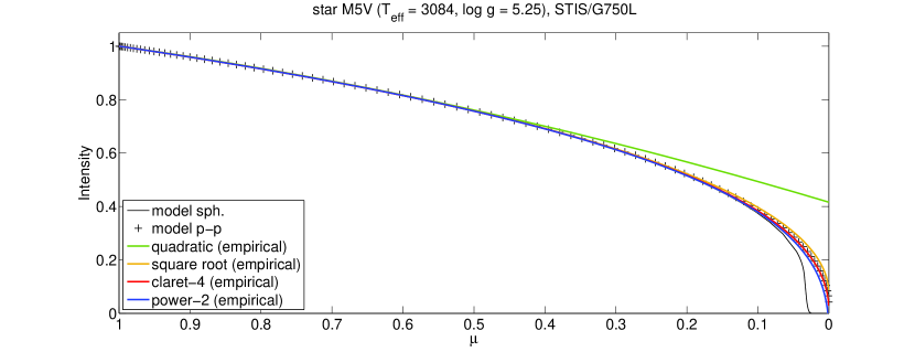
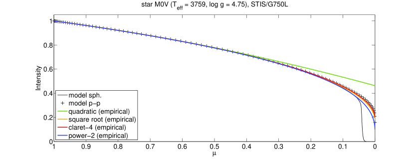
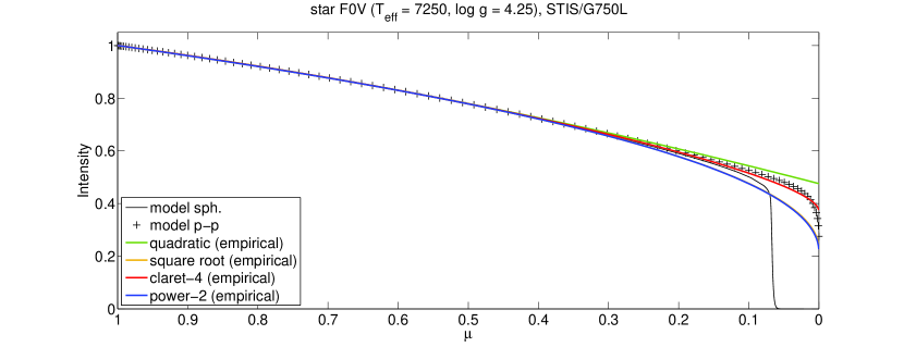
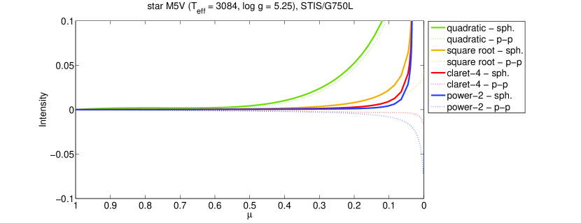
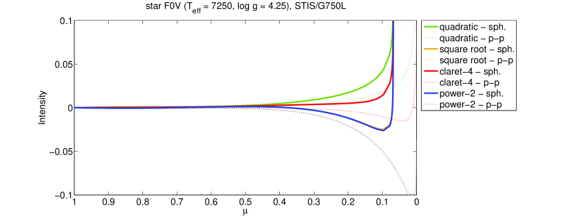
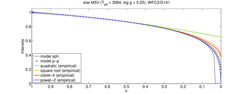
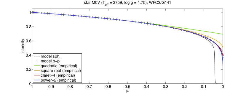
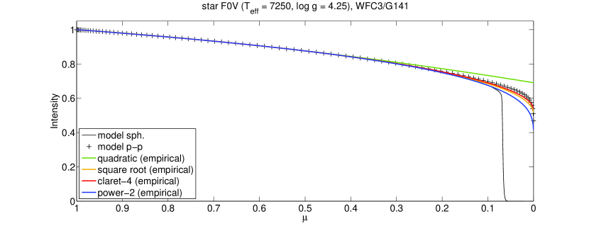
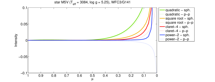
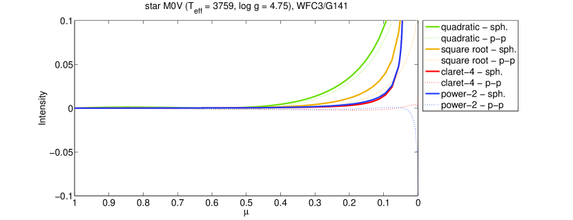
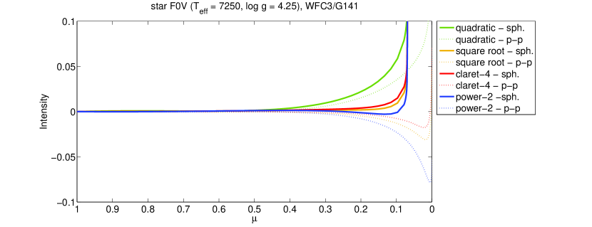
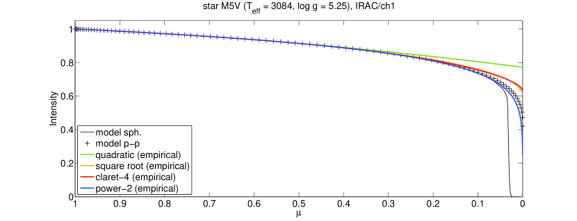
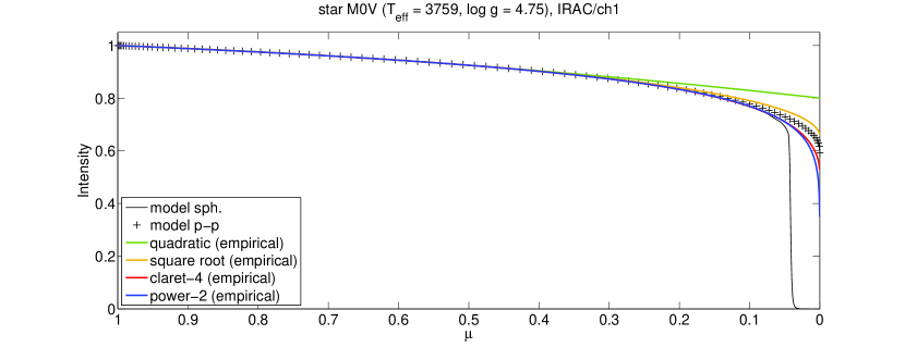
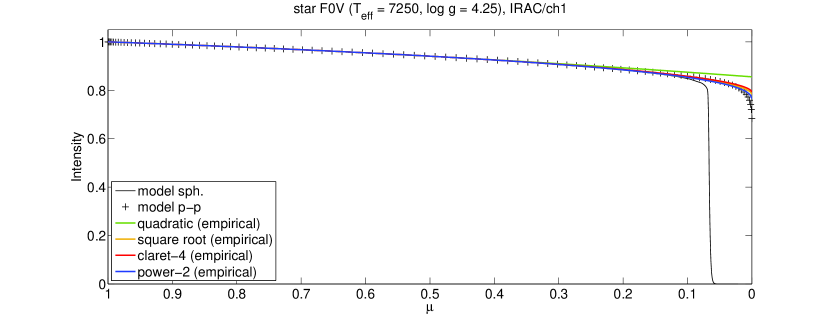
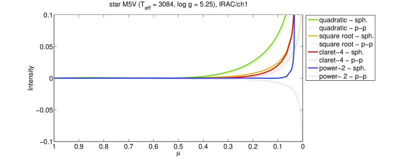
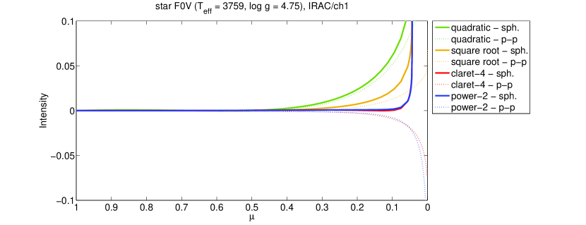
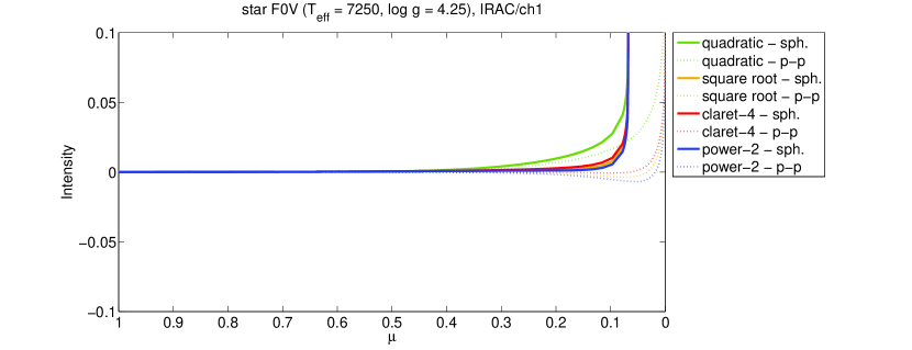
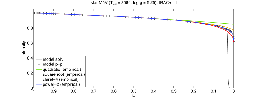
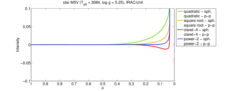
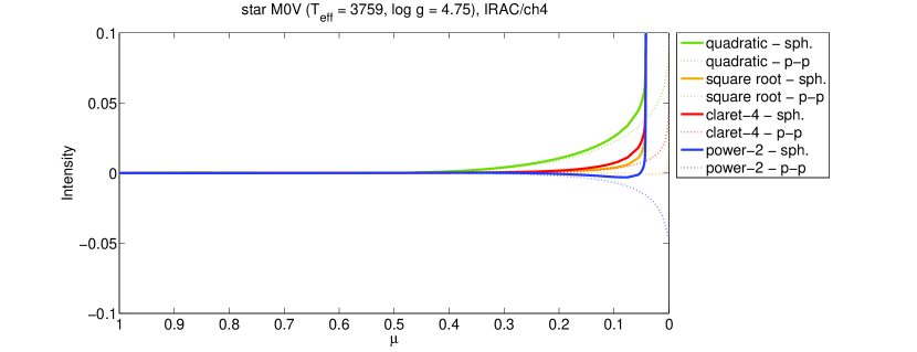
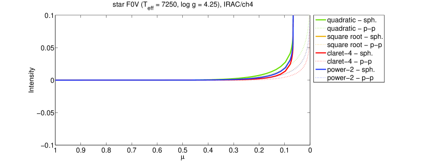
Figure 24: Top panels: Plane-parallel (black ‘+’) and spherical (black line) angular intensity vs. $\mu$. Parametric limb-darkening with empirical limb-darkening coefficients fitted to the transit light-curves with $b=0$, using quadratic (green), square-root (yellow), claret-4 (red), and power-2 (blue) law. Bottom panels: zoom of the residuals between parametric limb-darkening and spherical intensities (continuos lines), plane-parallel intensities (dashed lines).

Appendix B Supplemental figures: MCMC fitting results for inclined transits

This Appendix contains Figures 25–28 showing the histograms and chains for the inclined transits, analogous to those ones presented in Sections 5.1–5.2 for the edge-on transits (Figures 12–13 and 15–16).

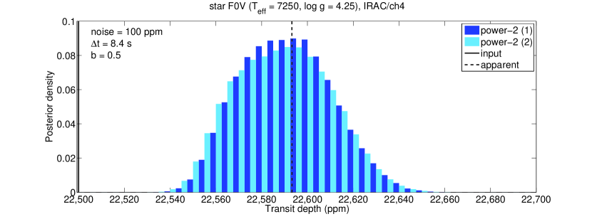
Figure 25: MCMC sampled posterior distributions of the transit depth for the inclined transit ($b=0.5$) in front of the F0 V model, IRAC/ch4 passband, with 100 ppm gaussian noise; fitting $p$, $a_{R}$, $i$, normalization factor, and power-2 limb-darkening coefficients. The histogram channels (blue and light-blue) are for two chains with 1 500 000 iterations; the channels are half-thick and shifted to improve their visualization. The input (black, continuous, vertical line) and expected (black, dashed, vertical line) transit depths are also indicated.

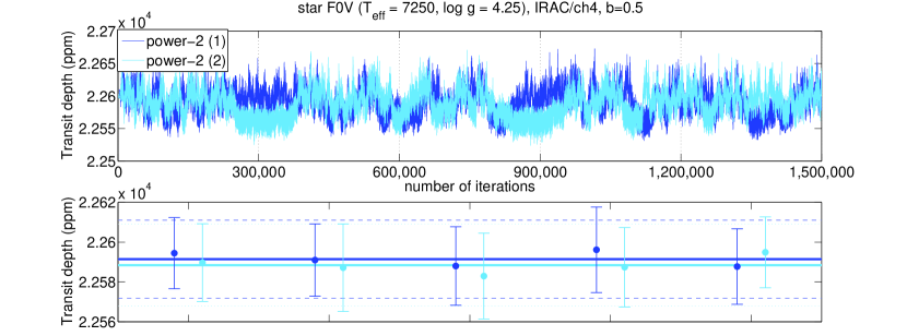
Figure 26: Top panel: transit depth chains for the inclined transit ($b=0.5$) in front of the F0 V model, IRAC/ch4 passband, with 100 ppm gaussian noise; fitting $p$, $a_{R}$, $i$, normalization factor and power-2 limb-darkening coefficients. Bottom panel: mean values and standard deviations calculated over fractional chains with 300 000 iterations; the horizontal lines indicate the mean values calculated over the whole chains (continuous lines), and the mean values plus or minus the standard deviations (dashed lines).

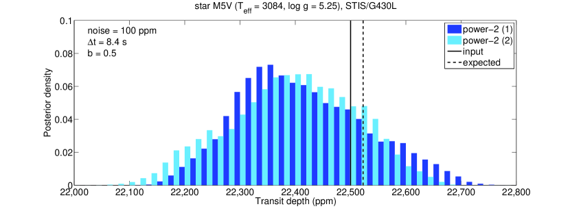
Figure 27: MCMC sampled posterior distributions of the transit depth for the inclined transit ($b=0.5$) in front of the M5 V model, STIS/G430L passband, with 100 ppm gaussian noise; fitting $p$, $a_{R}$, $i$, normalization factor and power-2 limb-darkening coefficients. The histogram channels (blue and light-blue) are for two chains with 1 500 000 iterations, using the power-2 law; the channels are half-thick and shifted to improve their visualization. The input (black, continuous, vertical line) and expected (black, dashed, vertical line) transit depths are also indicated.

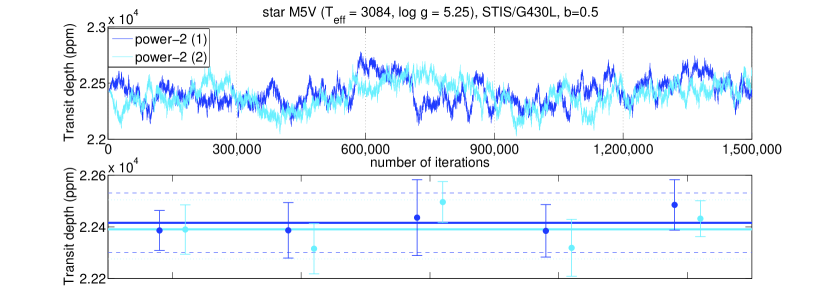
Figure 28: Top panel: transit depth chains for the inclined transit ($b=0.5$) in front of the M5 V model, STIS/G430L passband, with 100 ppm gaussian noise; fitting $p$, $a_{R}$, $i$, normalization factor and power-2 limb-darkening coefficients. Bottom panel: mean values and standard deviations calculated over fractional chains with 300 000 iterations; the horizontal lines indicate the mean values calculated over the whole chains (continuous lines), and the mean values plus or minus the standard deviations (dashed lines).

Appendix C Accuracy and precision of empirical limb-darkening models

In contrast to other transit parameters, the limb-darkening coefficients do not correspond directly to some physical property of the star-planet system. Also, for a given limb-darkening law, there exist sets of coefficients which are largely different but generate almost indistinguishable intensity profiles. Instead of studying their posterior distributions, it is more sensitive to calculate the chains of specific intensities at given $\mu$ values, then to compare, in the case of simulations, with the input limb-darkening profile.

Figure 29 shows the residuals in specific intensities obtained from the two light-curves relative to the F0 V model in the IRAC/ch4 passband (Section 5.1), one edge-on ($b=0$) and one inclined ($b=0.5$) transit, using the power-2 law. The error bars (i.e., the standard deviations of the intensity chains) are smaller than 0.2% for $\mu>0.4$, then increase up to $\gtrsim$1% near the edge of the disk. For the inclined transit, the error bars are larger by factors 1.0–2.4. The error bars of the predicted intensities along the steep drop-off, i.e. at $\mu\lesssim 0.08$, are not representative of the true errors, as the predictions may deviate from the input values by more than 10 $\sigma$.

We find that a good set of limb-darkening coefficients, which reproduces intensities close to those predicted by the intensity chains, can be obtained by taking medians of the coefficients chains. Figure 30 shows the intensity profiles estimated in this way, from light-curves with different noise realizations. They show, on average, the same bias obtained for the noiseless case (see Section 4.4).

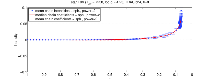
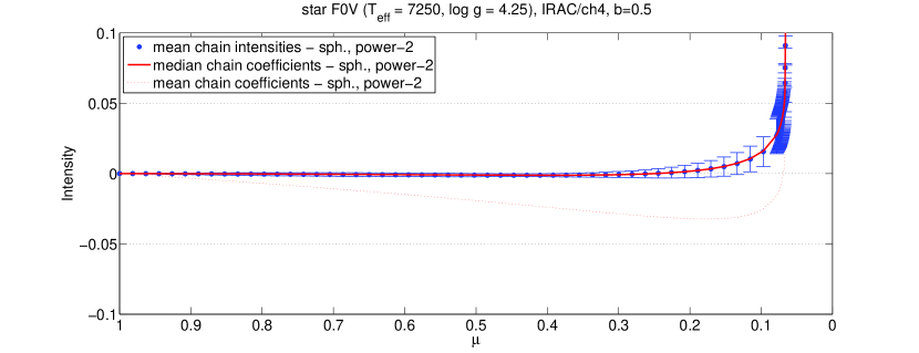
Figure 29: Top panel: residuals between power-2 empirical limb-darkening profile and the spherical intensities for the F0 V model, IRAC/ch4 passband, obtained from the edge-on transit with 100 ppm gaussian noise: estimates from the intensity chains (blue), model with median (red, continuous line) and mean (red, dotted line) chain values for the limb-darkening coefficients. Bottom panel: the same, from the inclined transit ($b=0.5$).

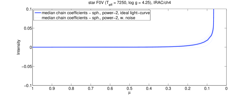
Figure 30: Residuals between power-2 empirical limb-darkening profile and the spherical intensities for the F0 V model, IRAC/ch4 passband, obtained from the edge-on transit without noise (blue, continuous line) and with 100 ppm gaussian noise (different noise time series, blue, dotted lines). Models are estimated by taking the median chain values for the limb-darkening coefficients.

Figures 31–32 report the analogous results obtained for the M5 V model in the STIS/G430L passband (Section 5.2). The error bars on the specific intensities are, in average, $\gtrsim$1.5 times larger than those obtained for the less limb darkened cases. Even in this case, the bias is similar to the one obtained for the noiseless case (see Section 4.4).

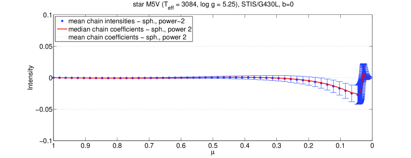
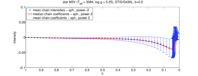
Figure 31: Top panel: residuals between power-2 empirical limb-darkening profile and the spherical intensities for the M5 V model, STIS/G430L passband, obtained from the edge-on transit with 100 ppm gaussian noise: estimates from the intensity chains (blue), model with median (red, continuous line) and mean (red, dotted line) chain values for the limb-darkening coefficients. Bottom panel: the same, from the inclined transit ($b=0.5$).

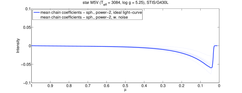
Figure 32: Residuals between power-2 empirical limb-darkening profile and the spherical intensities for the M5 V model, STIS/G430L passband, obtained from the edge-on transit without noise (blue, continuous line) and with 100 ppm gaussian noise (different noise time series, blue, dotted lines). Models are estimated by taking the mean chain values for the limb-darkening coefficients.

References

- Allard et al. (2012) Allard, F., Homeier, D. & Freytag, B. 2012, Philosophical Transactions of the Royal Society of London Series A, 370, 2765
- Aufdenberg et al. (2005) Aufdenberg, J. P., Ludwig, H.-G., & Kervella, P. 2005, ApJ, 633, 424
- Ballerini et al. (2012) Ballerini, P., Micela, G., Lanza, A. F., & Pagano, I. 2012, A&A, 539, A140
- Barnes (2009) Barnes, J. W. 2009, ApJ, 705, 683
- Barnes et al. (2011) Barnes, J. W., Linscott, E., & Shporer, A. 2011, ApJS, 197, 10
- Beichman et al. (2014) Beichman, C., Benneke, B., Knutson, H., Smith, R., Lagage, P.-O., Dressing, C., Latham, D., Lunine, J., Birkmann, S., Ferruit, P., Giardino, G., Kempton, E., Carey, S., Krick, J., Deroo, P. D., Mandell, A., Ressler, M. E., Shporer, A., Swain, M., Vasisht, G., Ricker, G., Bouwman, J., Crossfield, I., Greene, T., Howell, S., Christiansen, J., Ciardi, D., Clampin, M., Greenhouse, M., Sozzetti, A., Goudfrooij, P., Hines, D., Keyes, T., Lee, J., McCullough, P., Robberto, M., Stansberry, J., Valenti, J., Rieke, M., Rieke, G., Fortney, J., Bean, J., Kreidberg, L., Ehrenreich, D., Deming, D., Albert, L., Doyon, R., & Sing, D. 2014, PASP, 126, 1134
- Borucki et al. (2009) Borucki, W. J., Koch, D., Jenkins, J., Sasselov, D., Gilliland, R., Batalha, N., Latham, D. W., Caldwell, D., Basri, G., Brown, T., et al. 2009, Science, 325, 709
- Broomhall et al. (2009) Broomhall, A. M., Chaplin, W. J., Davies, G. R., Elsworth, Y., Fletcher, S. T., Hale, S. J., Miller, B., & New, R. 2009, MNRAS, 396, L100
- Charbonneau et al. (2002) Charbonneau, D., Brown, T. M., Noyes, R. W., & Gilliland, R. L. 2002, ApJ, 568, 377
- Chiavassa et al. (2016) Chiavassa, A., Caldas, A., Selsis, F., Leconte, J., Von Paris, P., Bordé, P., Magic, Z., Collet, R., & Asplund, M. 2016, arXiv1609.08966
- Claret (2000) Claret, A. 2000, A&A, 363, 1081
- Claret (2004) Claret, A. 2004, A&A, 428, 1001
- Claret (2008) Claret, A. 2008, A&A, 482, 259
- Claret (2009) Claret, A. 2009, A&A, 506, 1335
- Claret & Bloemen (2011) Claret, A., & Bloemen, S. 2011, A&A, 529, A75
- Claret et al. (2012) Claret, A., Hauschildt, P. H., & Witte, S. 2012, A&A, 546, A14
- Claret et al. (2012b) Claret, A. 2012, A&A, 538, A3
- Claret et al. (2013) Claret, A., Hauschildt, P. H., & Witte, S. 2013, A&A, 552, A16
- Claret et al. (2014) Claret, A., Dragomir, D., & Matthews, J. M. 2014, A&A, 567, A3
- Crouzet et al. (2014) Crouzet, N., McCullough, P. R., Deming, D., & Madhusudhan, N. 2014, ApJ, 795, 166
- Csizmadia et al. (2013) Csizmadia, S., Pasternacki, T., Dreyer, C., Cabrera, J., Erikson, A., & Rauer, H. 2013, A&A, 549, A9
- Danielski et al. (2014) Danielski, C., Deroo, P., Waldmann, I. P., Hollis, M. D. J., Tinetti, G., & Swain, M. R. 2014, ApJ, 785, 35
- Deming et al. (2013) Deming, D., Wilkins, A., McCullough, P., Burrows, A., Fortney, J. J., Agol, E., Dobbs-Dixon, I., Madhusudhan, N., Crouzet, N., Desert, J.-M., Gilliland, R. L., Haynes, K., Knutson, H. A., Line, M., Magic, Z., Mandell, A. M., Ranjan, S., Charbonneau, D., Clampin, M., Seager, S., & Showman, A. P. 2013, ApJ, 774, 95
- Devinney (1980) Devinney, Jr., E. J. 1980, BAAS, 12, 501
- Díaz-Cordovés & Giménez (1992) Diaz-Cordoves, J., & Gimenez, A. 1992, A&A, 259, 227
- Dominik (2004) Dominik, M. 2004, MNRAS, 353, 118
- Espinoza & Jordan (2015) Espinoza, N., & Jordán, A. 2015, MNRAS, 450, 1879
- Fields et al. (2003) Fields, D. L., Albrow, M. D., An, J., Beaulieu, J.-P., Caldwell, J. A. R., DePoy, D. L., Dominik, M., Gaudi, B. S., Gould, A., Greenhill, J., Hill, K., Jørgensen, U. G., Kane, S., Martin, R., Menzies, J., Pogge, R. W., Pollard, K. R., Sackett, P. D., Sahu, K. C., Vermaak, P., Watson, R., Williams, A., Glicenstein, J.-F., Hauschildt, P. H., 2003, ApJ, 596, 1305
- Fraine et al. (2014) Fraine, J., Deming, D., Benneke, B., Knutson, H., Jordán, A., Espinoza, N., Madhusudhan, N., Wilkins, A., & Todorov, K. 2014, Nature, 513, 526
- Gray & Corbally (2009) Gray, R. O., & Corbally, C. J. 2009, Stellar Spectral Classification, Princeton University Press, ISBN: 978-0-691-12510-7
- Grillmair et al. (2007) Grillmair, C. J., Charbonneau, D., Burrows, A., Armus, L., Stauffer, J., Meadows, V., Van Cleve, J., & Levine, D. 2007, ApJ, 658, L115
- Grillmair et al. (2008) Grillmair, C. J., Burrows, A., Charbonneau, D., Armus, L., Stauffer, J., Meadows, V., van Cleve, J., von Braun, K., & Levine, D. 2008, Nature, 456, 767
- Hayek et al. (2012) Hayek, W., Sing, D., Pont, F. & Asplund, M. 2012, A&A, 539, A102
- Hébrard et al. (2013) Hébrard, G., Almenara, J.-M., Santerne, A., Deleuil, M., Damiani, C., Bonomo, A. S., Bouchy, F., Bruno, G., Díaz, R. F., Montagnier, G., & Moutou, C. 2013, A&A, 554, A114
- Herrero et al. (2015) Herrero, E., Ribas, I., & Jordi, C. 2015, Experimental Astronomy, 40, 695
- Hestroffer (1997) Hestroffer, D. 1997, A&A, 327, 199
- Heyrovský (2007) Heyrovský, D. 2007, ApJ, 656, 483
- Howarth (2011) Howarth, I. D. 2011, MNRAS, 418, 1165
- Howarth (2011b) Howarth, I. D. 2011, MNRAS, 413, 1515
- Howarth & Morello (2017) Howarth, I. D., & Morello, G. 2017, MNRAS, 470, 932
- Kipping (2009) Kipping, D. M. 2009, MNRAS, 392, 181
- Kipping (2009b) Kipping, D. M. 2009, MNRAS, 396, 1797
- Kipping & Tinetti (2010) Kipping, D. M., & Tinetti, G. 2010, MNRAS, 407, 2589
- Kipping & Bakos (2011) Kipping, D., & Bakos, G. 2011, ApJ, 730, 50
- Kipping & Bakos (2011b) Kipping, D., & Bakos, G. 2011, ApJ, 733, 36
- Kipping (2014) Kipping, D. M. 2014, MNRAS, 444, 2263
- Kjeldsen & Bedding (2011) Kjeldsen, H., & Bedding, T. R. 2011, A&A, 529, L8
- Knutson et al. (2014) Knutson, H. A., Benneke, B., Deming, D., & Homeier, D. 2014, Nature, 505, 66
- Knutson et al. (2014b) Knutson, H. A., Dragomir, D., Kreidberg, L., Kempton, E. M. R., McCullough, P. R., Fortney, J. J., Bean, J. L., Gillon, M., Homeier, D., Howard, A. W. 2014, ApJ, 794, 155
- Kopal (1950) Kopal, Z. 1950, Harvard College Observatory Circular, 454, 1
- Kreidberg et al. (2014) Kreidberg, L., Bean, J. L., Désert, J.-M., Line, M. R., Fortney, J. J., Madhusudhan, N., Stevenson, K. B., Showman, A. P., Charbonneau, D., McCullough, P. R., Seager, S., Burrows, A., Henry, G. W., Williamson, M., Kataria, T., & Homeier, D. 2014, ApJ, 793, L27
- Kreidberg et al. (2014b) Kreidberg, L., Bean, J. L., Désert, J.-M., Benneke, B., Deming, D., Stevenson, K. B., Seager, S., Berta-Thompson, Z., Seifahrt, A., & Homeier, D. 2014, Nature, 505, 69
- Kreidberg et al. (2015) Kreidberg, L., Line, M. R., Bean, J. L., Stevenson, K. B., Désert, J.-M., Madhusudhan, N., Fortney, J. J., Barstow, J. K., Henry, G. W., Williamson, M. H., & Showman, A. P. 2015, ApJ, 814, 66
- Kreidberg (2015) Kreidberg, L. 2015, PASP, 127, 1161
- Lane et al. (2001) Lane, B. F., Boden, A. F., & Kulkarni, S. F. 2001, ApJ, 551, L81
- Line et al. (2016) Line, M. R., Stevenson, K. B., Bean, J., Désert, J.-M., Fortney, J. J., Kreidberg, L., Madhusudhan, N., Showman, A. P., & Diamond-Lowe, H. 2016, AJ, 152, 203
- Loeb & Gaudi (2003) Loeb, A., & Gaudi, B. S. 2003, ApJ, 588, L117
- Magic et al. (2015) Magic, Z., Chiavassa, A., Collet, R. & Asplund, M. 2015, A&A, 573, A90
- Mandel & Agol (2002) Mandel, K., & Agol, E. 2002, ApJ, 580, L171
- McCullough et al. (2014) McCullough, P. R., Crouzet, N., Deming, D., & Madhusudhan, N. 2014, ApJ, 791, 55
- Micela (2015) Micela, G. 2015, Experimental Astronomy, 40, 723
- Müller et al. (2013) Müller, H. M., Huber, K. F., Czesla, S., Wolter, U., & Schmitt, J. H. M. M. 2013, A&A, 560, A112
- Neilson & Lester (2013a) Neilson, H. R., & Lester, J. B. 2013, A&A, 554, A98
- Neilson & Lester (2013b) Neilson, H. R., & Lester, J. B. 2013, A&A, 556, A86
- Neilson et al. (2017) Neilson, H. R., McNeil, J. T., Ignace, R., & Lester, J. B. 2017, arXiv:1704.07376
- Pál (2008) , Pál, A. 2008, MNRAS, 390, 281
- Pfahl et al. (2008) Pfahl, E., Arras, P., & Paxton, B. 2008, ApJ, 679, 783
- Redfield et al. (2008) Redfield, S., Endl, M., Cochran, W. D., & Koesterke, L. 2008, ApJ, 673, L87
- Reeve & Howarth (2016) Reeve, D. C., & Howarth, I. D. 2016, MNRAS, 456, 1294
- Richardson et al. (2007) Richardson, L. J., Deming, D., Horning, K., Seager, S., & Harrington, J. 2007, Nature, 445, 892
- Sartoretti & Schneider (1999) Sartoretti, P., & Schneider, J. 1999, A&AS, 134, 553
- Scandariato & Micela (2015) Scandariato, G. & Micela, G. 2015, Experimental Astronomy, 40, 711
- Schneider et al. (2011) Schneider, J., Dedieu, C., Le Sidaner, P., Savalle, R., & Zolotukhin, I. 2011, A&A, 532, A79
- Shporer et al. (2012) Shporer, A., Brown, T., Mazeh, T., & Zucker, S. 2012, New A, 17, 309
- Sing (2010) Sing, D. K. 2010, A&A, 510, A21
- Snellen et al. (2008) Snellen, I. A. G., Albrecht, S., de Mooij, E. J. W., & Le Poole, R. S. 2008, A&A, 487, 357
- Snellen et al. (2009) Snellen, I. A. G., de Mooij, E. J. W., & Albrecht, S. 2009, Nature, 459, 543
- Southworth et al. (2004) Soutworth, J., Maxted, P. F. L., & Smalley, B. 2004, MNRAS, 351, 1277
- Southworth (2008) Soutworth, J. 2008, MNRAS, 386, 1644
- Stevenson et al. (2014) Stevenson, K. B., Désert, J.-M., Line, M. R., Bean, J. L., Fortney, J. J., Showman, A. P., Kataria, T., Kreidberg, L., McCullough, P. R., Henry, G. W., Charbonneau, D., Burrows, A., Seager, S., Madhusudhan, N., Williamson, M. H., & Homeier, D. 2014, Science, 346, 838
- Swain et al. (2008) Swain, M. R., Vasisht, G., & Tinetti, G. 2008, Nature, 452, 329
- Swain et al. (2009) Swain, M. R., Vasisht, G., Tinetti, G., Bouwman, J., Chen, P., Yung, Y., Deming, D., & Deroo, P. 2009, ApJ, 690, L114
- Swain et al. (2009b) Swain, M. R., Tinetti, G., Vasisht, G., Deroo, P., Griffith, C., Bouwman, J., Chen, P., Yung, Y., Burrows, A., Brown, L. R., Matthews, J., Rowe, J. F., Kuschnig, R., & Angerhausen, D. 2009, ApJ, 704, 1616
- Swain et al. (2010) Swain, M. R., Deroo, P., Griffith, C. A., Tinetti, G., Thatte, A., Vasisht, G., Chen, P., Bouwman, J., Crossfield, I. J., Angerhausen, D., Afonso, C., & Henning, T. 2010, Nature, 463, 637
- Tinetti et al. (2010) Tinetti, G., Deroo, P., Swain, M. R., Griffith, C. A., Vasisht, G., Brown, L. R., Burke, C., & McCullough, P. 2010, ApJ, 712, L139
- Tsiaras et al. (2016) Tsiaras, A., Rocchetto, M., Waldmann, I. P., Venot, O., Varley, R., Morello, G., Damiano, M., Tinetti, G., Barton, E. J., Yurchenko, S. N., & Tennyson, J. 2016, ApJ, 820, 99
- Tsiaras et al. (2016b) Tsiaras, A., Waldmann, I. P., Rocchetto, M., Varley, R., Morello, G., Damiano, M., & Tinetti, G. 2016, ApJ, 832, 202
- Van Cleve & Caldwell (2009) Van Cleve, J. E., & Caldwell, D. A. 2009, Kepler Instrument Handbook (KSCI-19033-001)
- Vidal-Madjar et al. (2003) Vidal-Madjar, A., Lecavelier des Etangs, A., Désert, J.-M., Ballester, G. E., Ferlet, R., Hébrard, G., & Mayor, M. 2003, Nature, 422, 143
- Vidal-Madjar et al. (2004) Vidal-Madjar, A., Désert, J.-M., Lecavelier des Etangs, A., Hébrard, G., Ballester, G. E., Ehrenreich, D., Ferlet, R., McConnell, J. C., Mayor, M., & Parkinson, C. D. 2004, ApJ, 604, L69
- von Zeipel (1924) von Zeipel, H. 1924, MNRAS, 84, 665
- Waldmann et al. (2012) Waldmann, I. P., Tinetti, G., Drossart, P., Swain, M. R., Deroo, P., & Griffith, C. A. 2012, ApJ, 744, 35
- Welsh et al. (2010) Welsh, W. F., Orosz, J. A., Seager, S., Fortney, J. J., Jenkins, J., Rowe, J. F., Koch, D., & Borucki, W. J. 2010, ApJ, 713, L145
- Wilson & Devinney (1971) Wilson, R. E., & Devinney, E. J. 2002, ApJ, 166, 605
- Witt (1995) Witt, H. J. 1995, ApJ, 449, 42
- Wittkowski et al. (2001) Wittkowski, M., Hummel, C. A., Johnston, K. J., Mozurkewich, D., Hajian, A. R., & White, N. M. 2001, A&A, 377, 981
- Wittkowski et al. (2004) Wittkowski, M., Aufdenberg, J. P., & Kervella, P. 2004, A&A, 413, 711
- Zub et al. (2011) Zub, M., Cassan, A., Heyrovský, D., Fouqué, P., Stempels, H. C., Albrow, M.D., Beaulieu, J.-P., Brillant, S., Christie, G. W., Kains, N., Kozłowski, S., Kubas, D., Wambsganss, J., Batista, V., Bennett, D. P., Cook, K., Coutures, C., Dieters, S., Dominik, M., Dominis Prester, D., Donatowicz, J., Greenhill, J., Horne, K., Jørgensen, U. G., Kane, S. R., Marquette, J.-B., Martin, R., Menzies, J., Pollard, K. R., Sahu, K. C., Vinter, C., Williams, A., Gould, A., Depoy, D. L., Gal-Yam, A., Gaudi, B. S., Han, C., Lipkin, Y., Maoz, D., Ofek, E. O., Park, B.-G., Pogge, R. W., McCormick, J., Udalski, A., Szymański, M. K., Kubiak, M., Pietrzyński, G., Soszyński, I., Szewczyk, O., Wyrzykowski, Ł., & PLANET Collaboration 2011, A&A, 525, A15
- Zucker et al. (2007) Zucker, S., Mazeh, T., & Alexander, T. 2007, ApJ, 670, 1326