Accelerating Stochastic Gradient Descent For Least Squares Regression

Abstract

There is widespread sentiment that fast gradient methods (e.g. Nesterov’s acceleration, conjugate gradient, heavy ball) are not effective for stochastic optimization due to their instability and error accumulation. Numerous works have attempted to quantify these instabilities in the face of either statistical or non-statistical errors (Paige, 1971; Proakis, 1974; Polyak, 1987; Greenbaum, 1989; Devolder et al., 2014). This work considers these issues for the case of stochastic approximation for the least squares regression problem, and our main result refutes this conventional wisdom by showing that acceleration can be made robust to statistical errors. In particular, this work introduces an accelerated stochastic gradient method that provably achieves the minimax optimal statistical risk faster than stochastic gradient descent. Critical to the analysis is a sharp characterization of accelerated stochastic gradient descent as a stochastic process. We hope this characterization gives insights towards the broader question of designing simple and effective accelerated stochastic methods for general convex and non-convex optimization problems.

1 Introduction

Stochastic gradient descent (SGD) is the workhorse algorithm for optimization in machine learning and stochastic approximation problems; improving its runtime dependencies is a central issue in large scale stochastic optimization that often arise in machine learning problems at scale (Bottou and Bousquet, 2007), where one can only resort to streaming algorithms.

This work examines these broader runtime issues for the special case of stochastic approximation in the following least squares regression problem:

$$\min_{\mathbf{x}\in\mathbb{R}^{d}}P(\mathbf{x}),\,\,\,\text{where, }P(\mathbf{x})\stackrel{{\scriptstyle\mathrm{def}}}{{=}}\tfrac{1}{2}\cdot\mathbb{E}_{(\mathbf{a},b)\sim\mathcal{D}}\left[(b-\left\langle\mathbf{x},\mathbf{a}\right\rangle)^{2}\right],$$ (1)

where we have access to a stochastic first order oracle, which, when provided with $\mathbf{x}$ as an input, returns a noisy unbiased stochastic gradient using a tuple $(\mathbf{a},b)$ sampled from $\mathcal{D}(\mathbb{R}^{d}\times\mathbb{R})$, with $d$ being the dimension of the problem. A query to the stochastic first-order oracle at $\mathbf{x}$ produces:

$$\widehat{\nabla}P(\mathbf{x})=\ -(b-\left\langle\mathbf{a},\mathbf{x}\right\rangle)\cdot\mathbf{a}.$$ (2)

Note $\mathbb{E}\left[\widehat{\nabla}P(\mathbf{x})\right]=\nabla P(\mathbf{x})$ (i.e. eq(2) is an unbiased estimate). Note that nearly all practical stochastic algorithms use sampled gradients of the specific form as in equation 2. We discuss differences to the more general stochastic first order oracle (Nemirovsky and Yudin, 1983) in section 1.4.

Algorithm Final error Runtime Memory Accelerated SVRG (Allen-Zhu, 2016) $\mathcal{O}\left(\frac{\sigma^{2}d}{n}\right)$ $({n+\sqrt{n{\kappa}}})d\log\bigg{(}{\frac{P(\mathbf{x}_{0})-P(\mathbf{x}_{*})}{(\sigma^{2}d/n)}}\bigg{)}$ $nd$ Streaming SVRG (Frostig et al., 2015b) Iterate Averaged SGD (Jain et al., 2016) $\mathcal{O}\left(\exp\left(\frac{-n}{{\kappa}}\right)\cdot\big{(}P(\mathbf{x}_{0})-P(\mathbf{x}_{*})\big{)}+\frac{\sigma^{2}d}{n}\right)$ ${nd}$ $\mathcal{O}(d)$ Accelerated Stochastic Gradient Descent (this paper) $\mathcal{O}^{*}\left(\exp\left(\frac{-n}{\sqrt{{\kappa}\widetilde{\kappa}}}\right)\big{(}P(\mathbf{x}_{0})-P(\mathbf{x}_{*})\big{)}\right)+\mathcal{O}\left(\frac{\sigma^{2}d}{n}\right)$ ${nd}$ $\mathcal{O}(d)$

Table 1: Comparison of this work to the best known non-asymptotic results (Frostig et al., 2015b; Jain et al., 2016) for the least squares stochastic approximation problem. Here, $d,n$ are the problem dimension, number of samples; ${\kappa}$, $\widetilde{\kappa}$ denote the condition number and statistical condition number of the distribution; $\sigma^{2}$, $P(\mathbf{x}_{0})-P(\mathbf{x}_{*})$ denote the noise level and initial excess risk, $\mathcal{O}^{*}$ hides lower order terms in $d,{\kappa},\widetilde{\kappa}$ (see section 2 for definitions and a proof for $\widetilde{\kappa}\leq{\kappa}$). Note that Accelerated SVRG (Allen-Zhu, 2016) is not a streaming algorithm.

Let $\mathbf{x}^{*}\stackrel{{\scriptstyle\textrm{def}}}{{=}}\arg\min_{\mathbf{x}}P(\mathbf{x})$ be a population risk minimizer. Given any estimation procedure which returns $\widehat{\mathbf{x}}_{n}$ using $n$ samples, define the excess risk (which we also refer to as the generalization error or the error) of $\widehat{\mathbf{x}}_{n}$ as $\mathbb{E}\left[P(\widehat{\mathbf{x}}_{n})\right]-P(\mathbf{x}^{*})$. Now, equipped a stochastic first-order oracle (equation (2)), our goal is to provide a computationally efficient (and streaming) estimation method whose excess risk is comparable to the optimal statistical minimax rate.

In the limit of large $n$, this minimax rate is achieved by the empirical risk minimizer (ERM), which is defined as follows. Given $n$ i.i.d. samples $\mathcal{S}_{n}=\{(\mathbf{a}_{i},b_{i})\}_{i=1}^{n}$ drawn from $\mathcal{D}$, define

$$\widehat{\mathbf{x}}_{n}^{\textrm{ERM}}\stackrel{{\scriptstyle\textrm{def}}}{{=}}\arg\min_{\mathbf{x}}P_{n}(\mathbf{x}),\textrm{ where }P_{n}(\mathbf{x})\stackrel{{\scriptstyle\textrm{def}}}{{=}}\frac{1}{n}\sum_{i=1}^{n}\tfrac{1}{2}\left(b_{i}-\mathbf{a}_{i}^{\top}\mathbf{x}\right)^{2},$$

where $\widehat{\mathbf{x}}_{n}^{\textrm{ERM}}$ denotes the ERM over the samples $\mathcal{S}_{n}$. For the case of additive noise models (i.e. where $b=\mathbf{a}^{\top}\mathbf{x}^{*}+\epsilon$, with $\epsilon$ being independent of $\mathbf{a}$), the minimax estimation rate is $d\sigma^{2}/n$ (Kushner and Clark, 1978; Polyak and Juditsky, 1992; Lehmann and Casella, 1998; van der Vaart, 2000), i.e.:

$$\lim_{n\to\infty}\frac{\mathbb{E}_{\mathcal{S}_{n}}[P(\widehat{\mathbf{x}}_{n}^{\textrm{ERM}})]-P(\mathbf{x}^{*})}{d\sigma^{2}/n} =1,$$ (3)

where $\sigma^{2}=\mathbb{E}\left[\epsilon^{2}\right]$ is the variance of the additive noise and the expectation is over the samples $\mathcal{S}_{n}$ drawn from $\mathcal{D}$. The seminal works of Ruppert (1988); Polyak and Juditsky (1992) proved that a certain averaged stochastic gradient method enjoys this minimax rate, in the limit. The question we seek to address is: how fast (in a non-asymptotic sense) can we achieve the minimax rate of $d\sigma^{2}/n$?

1.1 Review: Acceleration with Exact Gradients

Let us review results in convex optimization in the exact first-order oracle model. Running $t-$steps of gradient descent (Cauchy, 1847) with an exact first-order oracle yields the following guarantee:

$$P(\mathbf{x}_{t})-P(\mathbf{x}^{*})\leq\exp\big{(}-t/{\kappa}_{o}\big{)}\cdot\big{(}P(\mathbf{x}_{0})-P(\mathbf{x}^{*})\big{)},$$

where $\mathbf{x}_{0}$ is the starting iterate, ${\kappa}_{o}=\lambda_{\max}(\mathbf{H})/\lambda_{\min}(\mathbf{H})$ is the condition number of $P(.)$, where, $\lambda_{\max}(\mathbf{H}),\lambda_{\min}(\mathbf{H})$ are the largest and smallest eigenvalue of the hessian $\mathbf{H}=\nabla^{2}P(\mathbf{x})=\mathbb{E}\left[\mathbf{a}\mathbf{a}^{\top}\right]$. Thus gradient descent requires $\mathcal{O}({\kappa}_{o})$ oracle calls to solve the problem to a given target accuracy, which is sub-optimal amongst the class of methods with access to an exact first-order oracle (Nesterov, 2004). This sub-optimality can be addressed through Nesterov’s Accelerated Gradient Descent (Nesterov, 1983), which when run for t-steps, yields the following guarantee:

$$P(\mathbf{x}_{t})-P(\mathbf{x}^{*})\leq\exp\big{(}-t/\sqrt{{\kappa}_{o}}\big{)}\cdot\big{(}P(\mathbf{x}_{0})-P(\mathbf{x}^{*})\big{)},$$

which implies that $\mathcal{O}(\sqrt{{\kappa}_{o}})$ oracle calls are sufficient to achieve a given target accuracy. This matches the oracle lower bounds (Nesterov, 2004) that state that $\Theta(\sqrt{{\kappa}_{o}})$ calls to the exact first order oracle are necessary to achieve a given target accuracy. The conjugate gradient method (Hestenes and Stiefel, 1952) and heavy ball method (Polyak, 1964) are also known to obtain this convergence rate for solving a system of linear equations and for quadratic functions. These methods are termed fast gradient methods owing to the improvements offered by these methods over Gradient Descent.

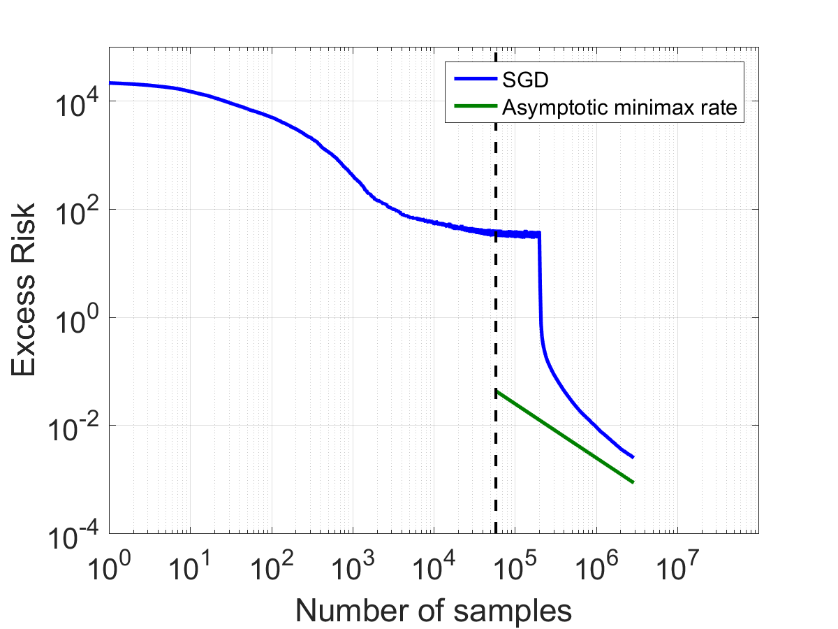
(a) Discrete distribution

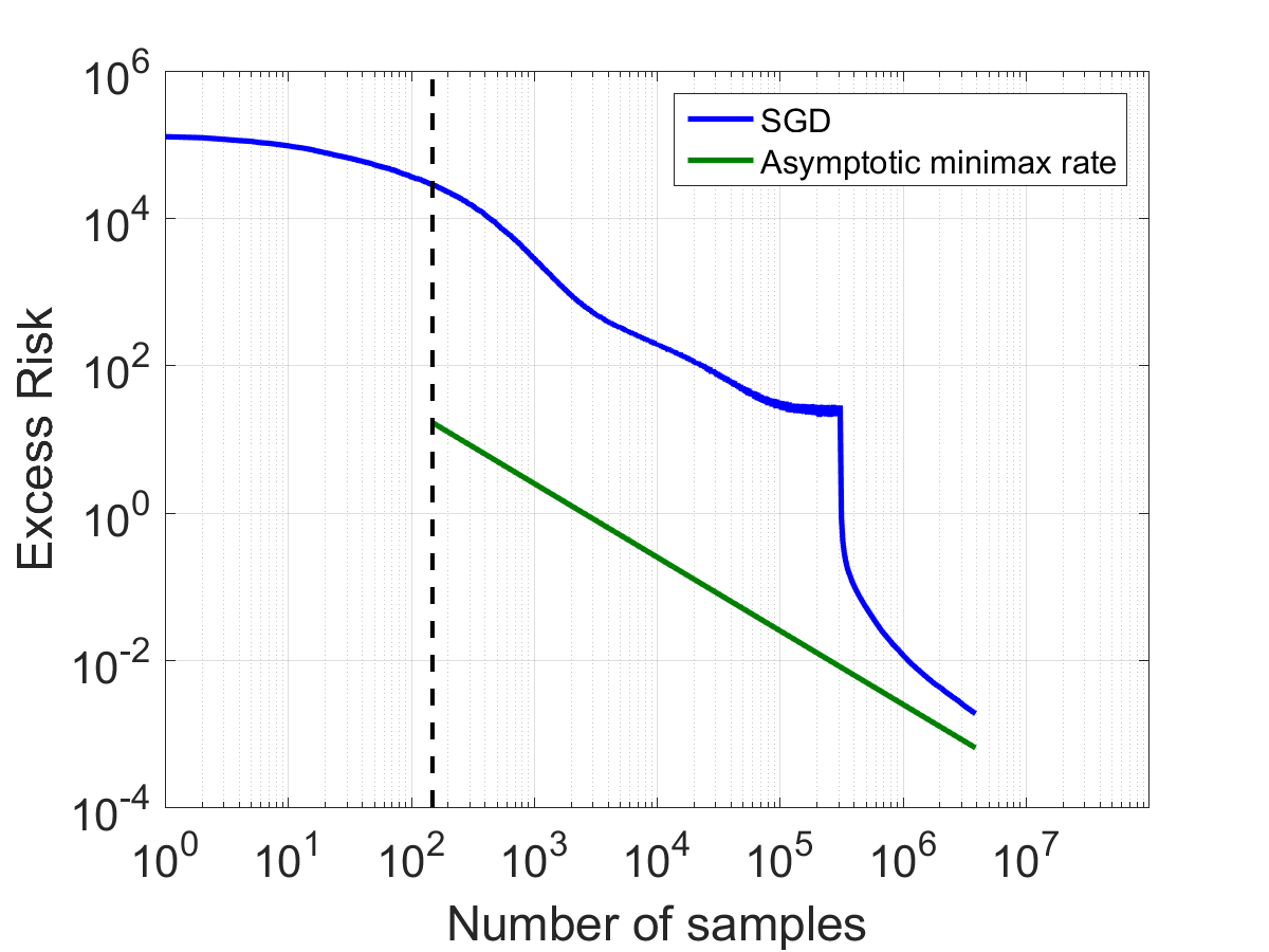
(b) Gaussian distribution

Figure 1: Plot of error vs number of samples for averaged SGD and the minimax risk for the discrete and Gaussian distributions with $d=50$, ${\kappa}\approx 10^{5}$ (see section 1.2 for details on the distribution). The kink in the SGD curve represents when the tail-averaging phase begins (Jain et al., 2016); this point is chosen appropriately. The green curves show the asymptotically optimal minimax rate of $d\sigma^{2}/n$. The vertical dashed line shows the sample size at which the empirical covariance, $\frac{1}{n}\sum_{i=1}^{n}\mathbf{a}_{i}\mathbf{a}_{i}^{\top}$, becomes full rank, which is shown at $\frac{1}{\min_{i}p_{i}}$ in the discrete case and $d$ in the Gaussian case. With fewer samples than this (i.e. before the dashed line), it is information theoretically not possible to guarantee non-trivial risk (without further assumptions). For the Gaussian case, note how the behavior of SGD is far from the dotted line; it is this behavior that one might hope to improve upon. See the text for a discussion.

This paper seeks to address the question: “Can we accelerate stochastic approximation in a manner similar to what has been achieved with the exact first order oracle model?”

1.2 A thought experiment: Is Accelerating Stochastic Approximation possible?

Let us recollect known results in stochastic approximation for the least squares regression problem (in equation 1). Running $n$-steps of tail-averaged SGD (Jain et al., 2016) (or, streaming SVRG (Frostig et al., 2015b)) provides an output $\widehat{\mathbf{x}}_{n}$ that satisfies the following excess risk bound:

$$\mathbb{E}\left[P(\widehat{\mathbf{x}}_{n})\right]-P(\mathbf{x}^{*})\leq\exp(-n/{\kappa})\cdot\big{(}P(\mathbf{x}_{0})-P(\mathbf{x}^{*})\big{)}+2\sigma^{2}d/n,$$ (4)

where ${\kappa}$ is the condition number of the distribution, which can be upper bounded as $L/\lambda_{\textrm{min}}(\mathbf{H})$, assuming that $\|\mathbf{a}\|\leq L$ with probability one (refer to section 2 for a precise definition of ${\kappa}$). Under appropriate assumptions, these are the best known rates under the stochastic first order oracle model (see section 1.4 for further discussion). A natural implication of the bound implied by averaged SGD is that with $\widetilde{\mathcal{O}}({\kappa})$ oracle calls (Jain et al., 2016) (where, $\widetilde{\mathcal{O}}(\cdot)$ hides $\log$ factors in $d,{\kappa}$), the excess risk attains (up to constants) the (asymptotic) minimax statistical rate. Note that the excess risk bounds in stochastic approximation consist of two terms: (a) bias: which represents the dependence of the generalization error on the initial excess risk $P(\mathbf{x}_{0})-P(\mathbf{x}^{*})$, and (b) the variance: which represents the dependence of the generalization error on the noise level $\sigma^{2}$ in the problem.

A precise question regarding accelerating stochastic approximation is: “is it possible to improve the rate of decay of the bias term, while retaining (up to constants) the statistical minimax rate?” The key technical challenge in answering this question is in sharply characterizing the error accumulation of fast gradient methods in the stochastic approximation setting. Common folklore and prior work suggest otherwise: several efforts have attempted to quantify instabilities in the face of statistical or non-statistical errors (Paige, 1971; Proakis, 1974; Polyak, 1987; Greenbaum, 1989; Roy and Shynk, 1990; Sharma et al., 1998; d’Aspremont, 2008; Devolder et al., 2013, 2014; Yuan et al., 2016). Refer to section 1.4 for a discussion on robustness of acceleration to error accumulation.

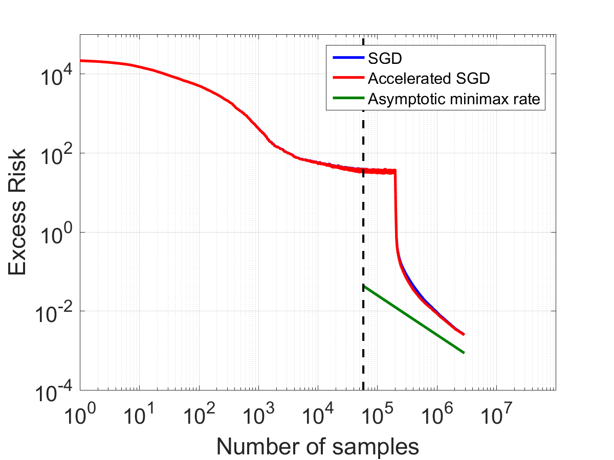
(a) Discrete distribution

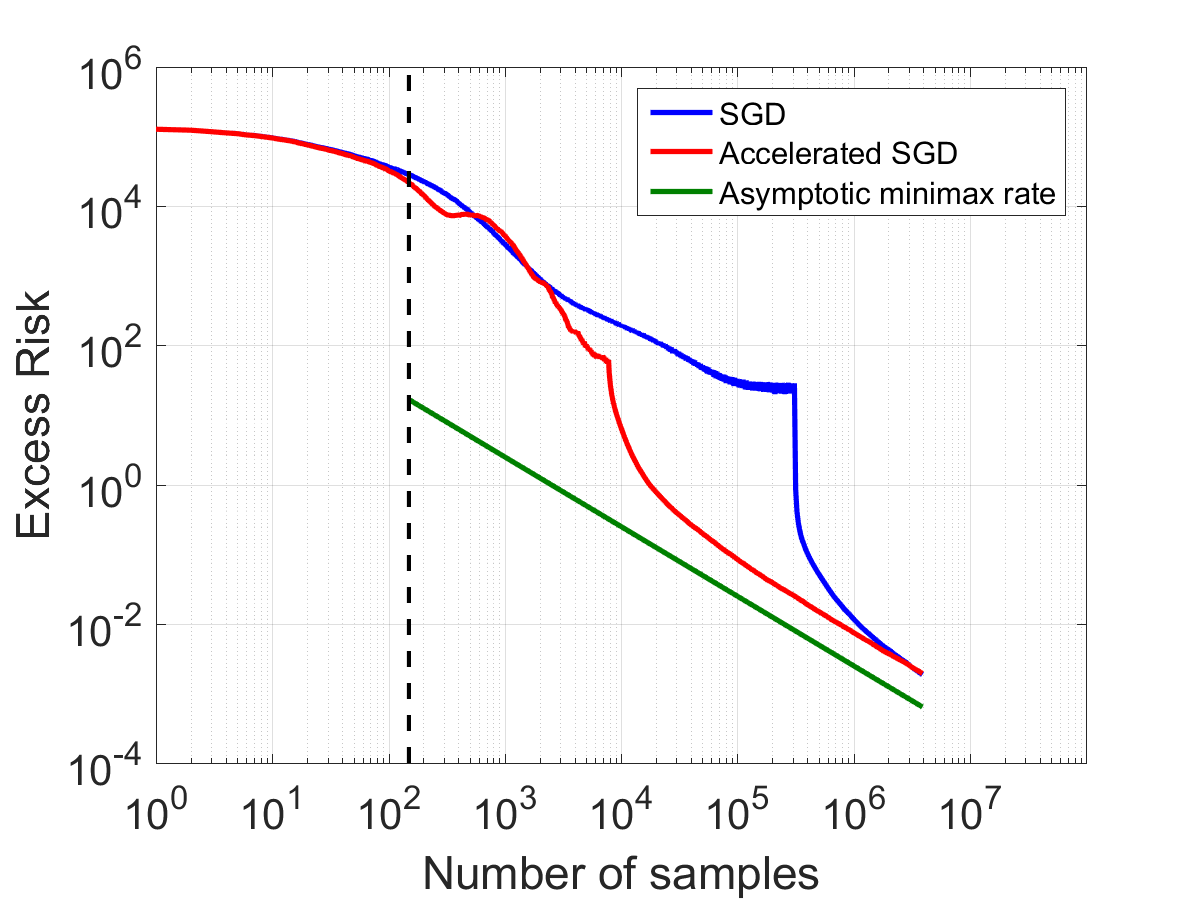
(b) Gaussian distribution

Figure 2: Plot of total error vs number of samples for averaged SGD, (this paper’s) accelerated SGD method and the minimax risk for the discrete and Gaussian distributions with $d=50,{\kappa}\approx 10^{5}$ (see section 1.2 for details on the distribution). For the discrete case, accelerated SGD degenerates to SGD, which nearly matches the minimax risk (when it becomes well defined). For the Gaussian case, accelerated SGD significantly improves upon SGD.

Optimistically, as suggested by the gains enjoyed by accelerated methods in the exact first order oracle model, we may hope to replace the $\widetilde{\mathcal{O}}({\kappa})$ oracle calls achieved by averaged SGD to $\widetilde{\mathcal{O}}(\sqrt{{\kappa}})$. We now provide a counter example, showing that such an improvement is not possible. Consider a (discrete) distribution $\mathcal{D}$ where the input $\mathbf{a}$ is the $i^{\textrm{th}}$ standard basis vector with probability $p_{i}$, $\forall\ i=1,2,...,d$. The covariance of $\mathbf{a}$ in this case is a diagonal matrix with diagonal entries $p_{i}$. The condition number of this distribution is ${\kappa}=\frac{1}{\min_{i}p_{i}}$. In this case, it is impossible to make non-trivial reduction in error by observing fewer than ${\kappa}$ samples, since with constant probability, we would not have seen the vector corresponding to the smallest probability.

On the other hand, consider a case where the distribution $\mathcal{D}$ is a Gaussian with a large condition number ${\kappa}$. Matrix concentration informs us that (with high probability and irrespective of how large ${\kappa}$ is) after observing $n=\mathcal{O}(d)$ samples, the empirical covariance matrix will be a spectral approximation to the true covariance matrix, i.e. for some constant $c>1$, $\mathbf{H}/c\preceq\frac{1}{n}\sum_{i=1}^{n}\mathbf{a}_{i}\mathbf{a}_{i}^{\top}\preceq c\mathbf{H}$. Here, we may hope to achieve a faster convergence rate, as information theoretically $\mathcal{O}(d)$ samples suffice to obtain a non-trivial statistical estimate (see Hsu et al. (2014) for further discussion).

Figure 1 shows the behavior of SGD in these cases; both are synthetic examples in $50-$dimensions, with a condition number ${\kappa}\approx 10^{5}$ and noise level $\sigma^{2}=100$. See the figure caption for more details.

These examples suggest that if acceleration is indeed possible, then the degree of improvement (say, over averaged SGD) must depend on distributional quantities that go beyond the condition number $\kappa$. A natural conjecture is that this improvement must depend on the number of samples required to spectrally approximate the covariance matrix of the distribution; below this sample size it is not possible to obtain any non-trivial statistical estimate due to information theoretic reasons. This sample size is quantified by a notion which we refer to as the statistical condition number $\widetilde{\kappa}$ (see section 2 for a precise definition and for further discussion about $\widetilde{\kappa}$). As we will see in section 2, we have $\widetilde{\kappa}\leq{\kappa}$, $\widetilde{\kappa}$ is affine invariant, unlike ${\kappa}$ (i.e. $\widetilde{\kappa}$ is invariant to linear transformations over $\mathbf{a}$).

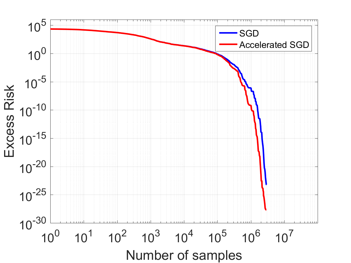
(a) Discrete distribution

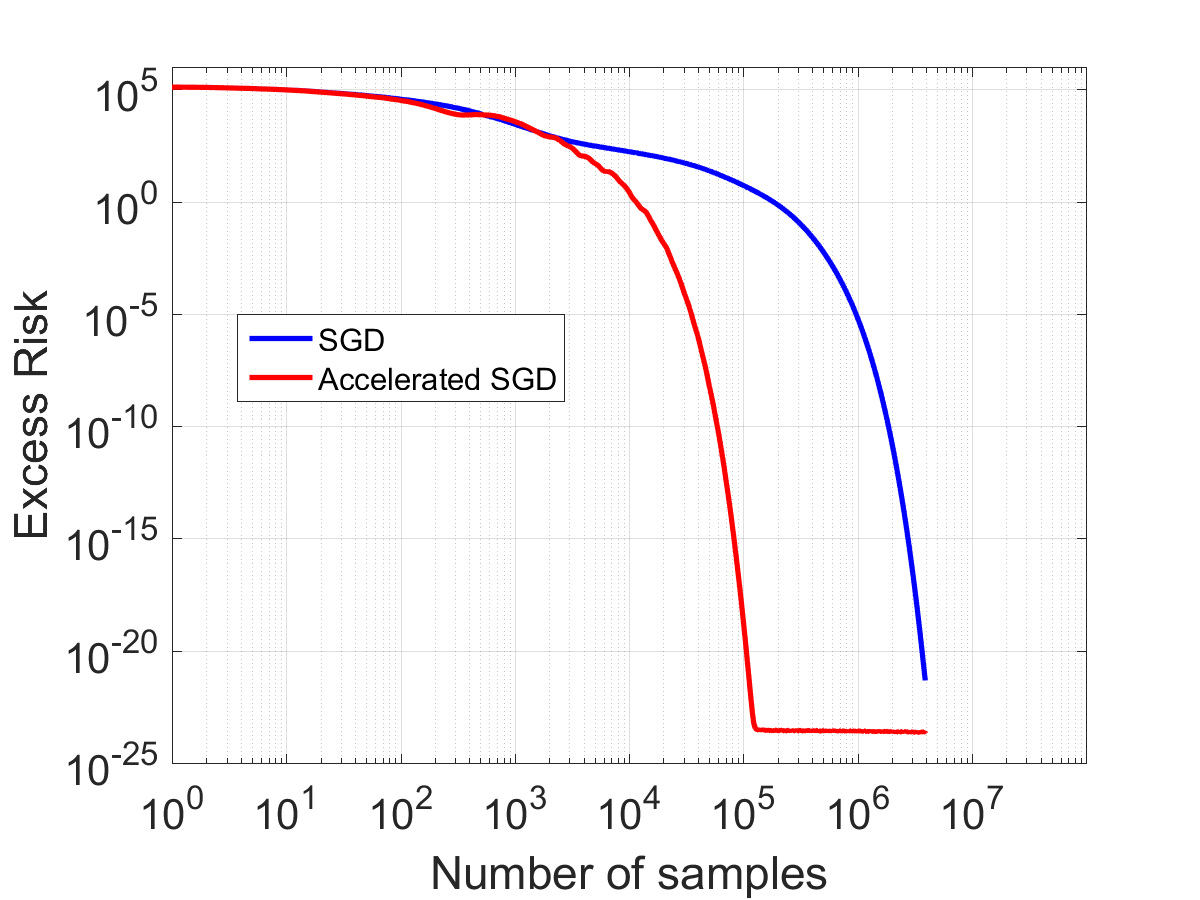
(b) Gaussian distribution

Figure 3: Comparison of averaged SGD with this paper’s accelerated SGD in the absence of noise ($\sigma^{2}=0$) for the Gaussian and Discrete distribution with $d=50,{\kappa}\approx 10^{5}$. Acceleration yields substantial gains over averaged SGD for the Gaussian case, while degenerating to SGD’s behavior for the discrete case. See section 1.2 for discussion.

1.3 Contributions

This paper introduces an accelerated stochastic gradient descent scheme, which can be viewed as a stochastic variant of Nesterov’s accelerated gradient method (Nesterov, 2012). As pointed out in Section 1.2, the excess risk of this algorithm can be decomposed into two parts namely, bias and variance. For the stochastic approximation problem of least squares regression, this paper establishes bias contraction at a geometric rate of $\mathcal{O}(1/\sqrt{{\kappa}\widetilde{\kappa}})$, improving over prior results (Frostig et al., 2015b; Jain et al., 2016),which prove a geometric rate of $\mathcal{O}(1/{\kappa})$, while retaining statistical minimax rates (up to constants) for the variance. Here ${\kappa}$ is the condition number and $\widetilde{\kappa}$ is the statistical condition number of the distribution, and a rate of $\mathcal{O}(1/\sqrt{{\kappa}\widetilde{\kappa}})$ is an improvement over $\mathcal{O}(1/{\kappa})$ since $\widetilde{\kappa}\leq{\kappa}$ (see Section 2 for definitions and a short proof of $\widetilde{\kappa}\leq{\kappa}$).

See Table 1 for a theoretical comparison. Figure 2 provides an empirical comparison of the proposed (tail-averaged) accelerated algorithm to (tail-averaged) SGD (Jain et al., 2016) on our two running examples. Our result gives improvement over SGD even in the noiseless (i.e. realizable) case where $\sigma=0$; this case is equivalent to the setting where we have a distribution over a (possibly infinite) set of consistent linear equations. See Figure 3 for a comparison on the case where $\sigma=0$.

On a more technical note, this paper introduces two new techniques in order to analyze the proposed accelerated stochastic gradient method: (a) the paper introduces a new potential function in order to show faster rates of decaying the bias, and (b) the paper provides a sharp understanding of the behavior of the proposed accelerated stochastic gradient descent updates as a stochastic process and utilizes this in providing a near-exact estimate of the covariance of its iterates. This viewpoint is critical in order to prove that the algorithm achieves the statistical minimax rate.

We use the operator viewpoint for analyzing stochastic gradient methods, introduced in Défossez and Bach (2015). This viewpoint was also used in Dieuleveut and Bach (2015); Jain et al. (2016).

1.4 Related Work

Non-asymptotic Stochastic Approximation:

Stochastic gradient descent (SGD) and its variants are by far the most widely studied algorithms for the stochastic approximation problem. While initial works (Robbins and Monro, 1951) considered the final iterate of SGD, later works (Ruppert, 1988; Polyak and Juditsky, 1992) demonstrated that averaged SGD obtains statistically optimal estimation rates. Several works provide non-asymptotic analyses for averaged SGD and variants (Bach and Moulines, 2011; Bach, 2014; Frostig et al., 2015b) for various stochastic approximation problems. For stochastic approximation with least squares regression Bach and Moulines (2013); Défossez and Bach (2015); Needell et al. (2016); Frostig et al. (2015b); Jain et al. (2016) provide non-asymptotic analysis of the behavior of SGD and its variants. Défossez and Bach (2015); Dieuleveut and Bach (2015) provide non-asymptotic results which achieve the minimax rate on the variance (where the bias is lower order, not geometric). Needell et al. (2016) achieves a geometric rate on the bias (and where the variance is not minimax). Frostig et al. (2015b); Jain et al. (2016) obtain both the minimax rate on the variance and a geometric rate on the bias, as seen in equation 4.

Acceleration and Noise Stability:

While there have been several attempts at understanding if it is possible to accelerate SGD , the results have been largely negative. With regards to acceleration with adversarial (non-statistical) errors in the exact first order oracle model, d’Aspremont (2008) provide negative results and Devolder et al. (2013, 2014) provide lower bounds showing that fast gradient methods do not improve upon standard gradient methods. There is also a series of works considering statistical errors. Polyak (1987) suggests that the relative merits of heavy ball (HB) method (Polyak, 1964) in the noiseless case vanish with noise unless strong assumptions on the noise model are considered; an instance of this is when the noise variance decays as the iterates approach the minimizer. The Conjugate Gradient (CG) method (Hestenes and Stiefel, 1952) is suggested to face similar robustness issues in the face of statistical errors (Polyak, 1987); this is in addition to the issues that CG is known to suffer from owing to roundoff errors (due to finite precision arithmetic) (Paige, 1971; Greenbaum, 1989). In the signal processing literature, where SGD goes by Least Mean Squares (LMS) (Widrow and Stearns, 1985), there have been efforts that date to several decades (Proakis, 1974; Roy and Shynk, 1990; Sharma et al., 1998) which study accelerated LMS methods (stochastic variants of CG/HB) in the same oracle model as the one considered by this paper (equation 2). These efforts consider the final iterate (i.e. no iterate averaging) of accelerated LMS methods with a fixed step-size and conclude that while it allows for a faster decay of the initial error (bias) (which is unquantified), their steady state behavior (i.e. variance) is worse compared to that of LMS. Yuan et al. (2016) considered a constant step size accelerated scheme with no iterate averaging in the same oracle model as this paper, and conclude that these do not offer any improvement over standard SGD. More concretely, Yuan et al. (2016) show that the variance of their accelerated SGD method with a sufficiently small constant step size is the same as that of SGD with a significantly larger step size. Note that none of the these efforts (Proakis, 1974; Roy and Shynk, 1990; Sharma et al., 1998; Yuan et al., 2016) achieve minimax error rates or quantify (any improvement whatsoever on the) rate of bias decay.

Oracle models and optimality:

With regards to notions of optimality, there are (at least) two lines of thought: one is a statistical objective where the goal is (on every problem instance) to match the rate of the statistically optimal estimator  (Anbar, 1971; Fabian, 1973; Kushner and Clark, 1978; Polyak and Juditsky, 1992); another is on obtaining algorithms whose worst case upper bounds (under various assumptions such as bounded noise) match the lower bounds provided in  Nemirovsky and Yudin (1983). The work of Polyak and Juditsky (1992) are in the former model, where they show that the distribution of the averaged SGD estimator matches, on every problem, that of the statistically optimal estimator, in the limit (under appropriate regularization conditions standard in the statistics literature, where the optimal estimator is often referred to as the maximum likelihood estimator/the empirical risk minimizer/an $M$-estimator (Lehmann and Casella, 1998; van der Vaart, 2000)). Along these lines, non-asymptotic rates towards statistically optimal estimators are given by Bach and Moulines (2013); Bach (2014); Défossez and Bach (2015); Dieuleveut and Bach (2015); Needell et al. (2016); Frostig et al. (2015b); Jain et al. (2016). This work can be seen as improving this non-asymptotic rate (to the statistically optimal estimation rate) using an accelerated method. As to the latter (i.e. matching the worst-case lower bounds in  Nemirovsky and Yudin (1983)), there are a number of positive results on using accelerated stochastic optimization procedures; the works of Lan (2008); Hu et al. (2009); Ghadimi and Lan (2012, 2013); Dieuleveut et al. (2016) match the lower bounds provided in Nemirovsky and Yudin (1983). We compare these assumptions and works in more detail.

In stochastic first order oracle models (see  Kushner and Clark (1978); Kushner and Yin (2003)), one typically has access to sampled gradients of the form:

$$\widehat{\nabla}P(\mathbf{x})=\nabla P(\mathbf{x})+\bm{\eta},$$ (5)

where varying assumptions are made on the noise $\bm{\eta}$. The worst-case lower bounds in Nemirovsky and Yudin (1983) are based on that $\bm{\eta}$ is bounded; the accelerated methods in Lan (2008); Hu et al. (2009); Ghadimi and Lan (2012, 2013); Dieuleveut et al. (2016) which match these lower bounds in various cases, all assume either bounded noise or, at least $\mathbb{E}\left[\|\bm{\eta}\|^{2}\right]$ is finite. In the least squares setting (such as the one often considered in practice and also considered in Polyak and Juditsky (1992); Bach and Moulines (2013); Défossez and Bach (2015); Dieuleveut and Bach (2015); Frostig et al. (2015b); Jain et al. (2016)), this assumption does not hold, since $\mathbb{E}\left[\|\bm{\eta}\|^{2}\right]$ is not bounded. To see this, $\bm{\eta}$ in our oracle model (equation 2) is:

$$\bm{\eta}=\widehat{\nabla}P(\mathbf{x})-\nabla P(\mathbf{x})=(\mathbf{a}\mathbf{a}^{\top}-\mathbf{H})(\mathbf{x}-\mathbf{x}^{*})-\epsilon\cdot\mathbf{a}$$ (6)

which implies that $\mathbb{E}\left[\|\bm{\eta}\|^{2}\right]$ is not uniformly bounded (unless additional assumptions are enforced to ensure that the algorithm’s iterates $\mathbf{x}$ lie within a compact set). Hence, the assumptions made in Hu et al. (2009); Ghadimi and Lan (2012, 2013); Dieuleveut et al. (2016) do not permit one to obtain finite $n$-sample bounds on the excess risk. Suppose we consider the case of $\epsilon=0$, i.e. where the additive noise is zero and $b=\mathbf{a}^{\top}\mathbf{x}^{*}$. For this case, this paper provides a geometric rate of convergence to the minimizer $\mathbf{x}^{*}$, while the results of Ghadimi and Lan (2012, 2013); Dieuleveut et al. (2016) at best indicate a $\mathcal{O}(1/n)$ rate. Finally, in contrast to all other existing work, our result is the first to provide finer distribution dependent characteristics of the improvements offered by accelerating SGD (e.g. refer to the Gaussian and discrete examples in section 1.2).

Acceleration and Finite Sums:

As a final remark, there have been results (Shalev-Shwartz and Zhang, 2014; Frostig et al., 2015a; Lin et al., 2015; Lan and Zhou, 2015; Allen-Zhu, 2016) that provide accelerated rates for offline stochastic optimization which deal with minimizing sums of convex functions; these results are almost tight due to matching lower bounds (Lan and Zhou, 2015; Woodworth and Srebro, 2016). These results do not immediately translate into rates on the generalization error. Furthermore, these algorithms are not streaming, as they require making multiple passes over a dataset stored in memory. Refer to Frostig et al. (2015b) for more details.

2 Main Results

We now provide our assumptions and main result, before which, we have some notation. For a vector $\mathbf{x}\in\mathbb{R}^{d}$ and a positive semi-definite matrix $\mathbf{S}\in\mathbb{R}^{d\times d}$ (i.e. $\mathbf{S}\succeq 0$), denote $\|\mathbf{x}\|^{2}_{\mathbf{S}}\stackrel{{\scriptstyle\textrm{def}}}{{=}}\mathbf{x}^{\top}\mathbf{S}\mathbf{x}$.

2.1 Assumptions and Definitions

Let $\mathbf{H}$ denote the second moment matrix of the input, which is also the hessian $\nabla^{2}P(\mathbf{x})$ of (1):

$$\mathbf{H}\stackrel{{\scriptstyle\textrm{def}}}{{=}}\mathbb{E}_{(\mathbf{a},b)\sim\mathcal{D}}\left[\mathbf{a}\otimes\mathbf{a}\right]=\nabla^{2}P(\mathbf{x}).$$

Furthermore, let the fourth moment tensor $\mathcal{M}$ of the inputs $\mathbf{a}\sim\mathcal{D}$ is defined as:

$$\mathcal{M}=\mathbb{E}_{(\mathbf{a},b)\sim\mathcal{D}}\left[\mathbf{a}\otimes\mathbf{a}\otimes\mathbf{a}\otimes\mathbf{a}\right].$$

1. Finite second and fourth moment: The second moment matrix $\mathbf{H}$ and the fourth moment tensor $\mathcal{M}$ exist and are finite.

2. Positive Definiteness: The second moment matrix $\mathbf{H}$ is strictly positive definite, i.e. $\mathbf{H}\succ 0$.

We assume $\mathbf{(\mathcal{A}1)}$ and $\mathbf{(\mathcal{A}2)}$. $\mathbf{(\mathcal{A}2)}$ implies that $P(\mathbf{x})$ is strongly convex and admits a unique minimizer $\mathbf{x}^{*}$. Denote the noise $\epsilon$ in a sample $(\mathbf{a},b)\sim\mathcal{D}$ as: $\epsilon\stackrel{{\scriptstyle\textrm{def}}}{{=}}b-\left\langle\mathbf{a},\mathbf{x}^{*}\right\rangle$. First order optimality conditions of $\mathbf{x}^{*}$ imply

$$\nabla P(\mathbf{x}^{*})=\mathbb{E}\left[\epsilon\cdot\mathbf{a}\right]=0.$$

Let $\mathbf{\Sigma}$ denote the covariance of gradient at optimum $\mathbf{x}^{*}$ (or noise covariance matrix),

$$\mathbf{\Sigma}\stackrel{{\scriptstyle\mathrm{def}}}{{=}}\mathbb{E}_{(\mathbf{a},b)\sim\mathcal{D}}\left[\widehat{\nabla}P(\mathbf{x}^{*})\otimes\widehat{\nabla}P(\mathbf{x}^{*})\right]=\mathbb{E}_{(\mathbf{a},b)\sim\mathcal{D}}\left[\epsilon^{2}\cdot\mathbf{a}\otimes\mathbf{a}\right].$$

We define the noise level $\sigma^{2}$, condition number ${\kappa}$, statistical condition number $\widetilde{\kappa}$ below.
Noise level: The noise level is defined to be the smallest positive number $\sigma^{2}$ such that

$$\mathbf{\Sigma}\preceq\sigma^{2}\mathbf{H}.$$

The noise level $\sigma^{2}$ quantifies the amount of noise in the stochastic gradient oracle and has been utilized in previous work (e.g., see Bach and Moulines (2011, 2013)) for providing non-asymptotic bounds for the stochastic approximation problem. In the homoscedastic (additive noise/well specified) case, where $\epsilon$ is independent of the input $\mathbf{a}$, this condition is satisfied with equality, i.e. $\mathbf{\Sigma}=\sigma^{2}\ \mathbf{H}$ with $\sigma^{2}=\mathbb{E}\left[\epsilon^{2}\right]$.
Condition number: Let

$$\mu\stackrel{{\scriptstyle\mathrm{def}}}{{=}}\lambda_{\textrm{min}}(\mathbf{H}).$$

$\mu>0$ by $\mathbf{(\mathcal{A}2)}$. Now, let $R^{2}$ be the smallest positive number such that

$$\mathbb{E}\left[\|\mathbf{a}\|^{2}\ \mathbf{a}\mathbf{a}^{\top}\right]\preceq R^{2}\ \mathbf{H}.$$

. The condition number ${\kappa}$ of the distribution $\mathcal{D}$ (Défossez and Bach, 2015; Jain et al., 2016) is

$${\kappa}\stackrel{{\scriptstyle\mathrm{def}}}{{=}}{R^{2}}/{\mu}.$$

Statistical condition number: The statistical condition number $\widetilde{\kappa}$ is defined as the smallest positive number such that

$$\mathbb{E}\left[\left\|\mathbf{a}\right\|_{\mathbf{H}^{-1}}^{2}\mathbf{a}\mathbf{a}^{\top}\right]\preceq\widetilde{\kappa}\ \mathbf{H}.$$

Remarks on $\widetilde{\kappa}$ and ${\kappa}$: Unlike ${\kappa}$, it is straightforward to see that $\widetilde{\kappa}$ is affine invariant (i.e. unchanged with linear transformations over $\mathbf{a}$). Since $\mathbb{E}\left[\left\|\mathbf{a}\right\|_{\mathbf{H}^{-1}}^{2}\mathbf{a}\mathbf{a}^{\top}\right]\preceq\frac{1}{\mu}\mathbb{E}\left[\left\|\mathbf{a}\right\|_{2}^{2}\mathbf{a}\mathbf{a}^{\top}\right]\preceq{\kappa}\mathbf{H}$, we note $\widetilde{\kappa}\leq{\kappa}$. For the discrete case (from Section 1.2), it is straightforward to see that both ${\kappa}$ and $\widetilde{\kappa}$ are equal to $1/\min_{i}p_{i}$. In contrast, for the Gaussian case (from Section 1.2), $\widetilde{\kappa}$ is $\mathcal{O}(d)$, while ${\kappa}$ is $\mathcal{O}(\textrm{Trace}(\mathbf{H})/\mu)$ which may be arbitrarily large (based on choice of the coordinate system).

$\widetilde{\kappa}$ governs how many samples $\mathbf{a}_{i}$ require to be drawn from $\mathcal{D}$ so that the empirical covariance is spectrally close to $\mathbf{H}$, i.e. for some constant $c>1$, $\mathbf{H}/c\preceq\frac{1}{n}\sum_{i=1}^{n}\mathbf{a}_{i}\mathbf{a}_{i}^{\top}\preceq c\mathbf{H}$. In comparison to the matrix Bernstein inequality where stronger (yet related) moment conditions are assumed in order to obtain high probability results, our results hold only in expectation (refer to Hsu et al. (2014) for this definition, wherein $\widetilde{\kappa}$ is referred to as bounded statistical leverage in theorem $1$ and remark $1$).

Algorithm 1 (Tail-Averaged) Accelerated Stochastic Gradient Descent (ASGD)

0:  $n$ oracle calls 2, initial point $\mathbf{x}_{0}=\mathbf{v}_{0}$, Unaveraged (burn-in) phase $t$, Step size parameters $\alpha,\beta,\gamma,\delta$

1:  for $j=1,\cdots n$ do

2:     $\mathbf{y}_{j-1}\leftarrow\alpha\mathbf{x}_{j-1}+(1-\alpha)\mathbf{v}_{j-1}$

3:     $\mathbf{x}_{j}\leftarrow\mathbf{y}_{j-1}-\delta\widehat{\nabla}P(\mathbf{y}_{j-1})$

4:     $\mathbf{z}_{j-1}\leftarrow\beta\mathbf{y}_{j-1}+(1-\beta)\mathbf{v}_{j-1}$

5:     $\mathbf{v}_{j}\leftarrow\mathbf{z}_{j-1}-\gamma\widehat{\nabla}P(\mathbf{y}_{j-1})$

6:  end for

6:  $\bar{\mathbf{x}}_{t,n}\leftarrow\frac{1}{n-t}\sum_{j=t+1}^{n}\mathbf{x}_{j}$

2.2 Algorithm and Main Theorem

Algorithm 1 presents the pseudo code of the proposed algorithm. ASGD can be viewed as a variant of Nesterov’s accelerated gradient method (Nesterov, 2012), working with a stochastic gradient oracle (equation 2) and with tail-averaging the final $n-t$ iterates. The main result now follows:

Theorem 1.

Suppose  $\mathbf{(\mathcal{A}1)}$ and  $\mathbf{(\mathcal{A}2)}$ hold. Set $\alpha=\frac{3\sqrt{5}\cdot\sqrt{{\kappa}\widetilde{\kappa}}}{1+3\sqrt{5}\cdot\sqrt{{\kappa}\widetilde{\kappa}}},\beta=\frac{1}{9\sqrt{{\kappa}\widetilde{\kappa}}},\gamma=\frac{1}{3\sqrt{5}\cdot\mu\sqrt{{\kappa}\widetilde{\kappa}}},\delta=\frac{1}{5R^{2}}$. After $n$ calls to the stochastic first order oracle (equation 2), ASGD outputs $\bar{\mathbf{x}}_{t,n}$ satisfying:

$$\mathbb{E}\left[P(\bar{\mathbf{x}}_{t,n})\right]-P(\mathbf{x}^{*})\leq\underbrace{C\cdot\frac{({\kappa}\widetilde{\kappa})^{9/4}d{\kappa}}{(n-t)^{2}}\cdot\exp\bigg{(}\frac{-t}{9\sqrt{{\kappa}\widetilde{\kappa}}}\bigg{)}\cdot\big{(}P(\mathbf{x}_{0})-P(\mathbf{x}^{*})\big{)}}_{\text{Leading order bias error}}+\underbrace{5\frac{\sigma^{2}d}{n-t}}_{\text{Leading order variance error}}+$$

$$\underbrace{C\cdot({\kappa}\widetilde{\kappa})^{5/4}d{\kappa}\cdot\exp\left(\frac{-n}{9\sqrt{{\kappa}\widetilde{\kappa}}}\right)\big{(}P(\mathbf{x}_{0})-P(\mathbf{x}^{*})\big{)}}_{\text{Exponentially vanishing lower order bias term}}+\underbrace{C\cdot\frac{\sigma^{2}d}{(n-t)^{2}}\sqrt{{\kappa}\widetilde{\kappa}}}_{\text{Lower order variance error term}}+$$

$${\small\underbrace{C\cdot\exp\bigg{(}{-\frac{n}{9\sqrt{{\kappa}\widetilde{\kappa}}}}\bigg{)}\cdot\bigg{(}\sigma^{2}d\cdot({\kappa}\widetilde{\kappa})^{7/4}+\frac{\sigma^{2}d}{(n-t)^{2}}\cdot({\kappa}\widetilde{\kappa})^{7/2}\widetilde{\kappa}\bigg{)}+C\cdot\frac{\sigma^{2}d}{n-t}({\kappa}\widetilde{\kappa})^{11/4}\exp\bigg{(}{-\frac{(n-t-1)}{30\sqrt{{\kappa}\widetilde{\kappa}}}}\bigg{)}}_{\text{Exponentially vanishing lower order variance error terms}}},$$

where $C$ is a universal constant, $\sigma^{2}$, ${\kappa}$ and $\widetilde{\kappa}$ are the noise level, condition number and statistical condition number respectively.

The following corollary holds if the iterates are tail-averaged over the last $n/2$ samples and $n>\mathcal{O}(\sqrt{{\kappa}\widetilde{\kappa}}\log(d{\kappa}\widetilde{\kappa}))$. The second condition lets us absorb lower order terms into leading order terms.

Corollary 2.

Assume the parameter settings of theorem 1 and let $t=\lfloor n/2\rfloor$ and $n>C^{\prime}\sqrt{{\kappa}\widetilde{\kappa}}\log(d{\kappa}\widetilde{\kappa})$ (for an appropriate universal constants $C,C^{\prime}$). We have that with $n$ calls to the stochastic first order oracle, ASGD outputs a vector $\bar{\mathbf{x}}_{t,n}$ satisfying:

$$\mathbb{E}\left[P(\bar{\mathbf{x}}_{t,n})\right]-P(\mathbf{x}^{*})\leq C\cdot\exp\bigg{(}-\frac{n}{20\sqrt{{\kappa}\widetilde{\kappa}}}\bigg{)}\cdot\big{(}P(\mathbf{x}_{0})-P(\mathbf{x}^{*})\big{)}+11\frac{\sigma^{2}d}{n}.$$

A few remarks about the result of theorem 1 are due: (i) ASGD decays the initial error at a geometric rate of $\mathcal{O}(1/\sqrt{{\kappa}\widetilde{\kappa}})$ during the unaveraged phase of $t$ iterations, which presents the first improvement over the $\mathcal{O}\left(1/{\kappa}\right)$ rate offered by SGD (Robbins and Monro, 1951)/averaged SGD (Polyak and Juditsky, 1992; Jain et al., 2016) for the least squares stochastic approximation problem, (ii) the second term in the error bound indicates that ASGD obtains (up to constants) the minimax rate once $n>\mathcal{O}(\sqrt{{\kappa}\widetilde{\kappa}}\log(d{\kappa}\widetilde{\kappa}))$. Note that this implies that Theorem 1 provides a sharp non-asymptotic analysis (up to $\log$ factors) of the behavior of Algorithm 1.

2.3 Discussion and Open Problems

A challenging problem in this context is in formalizing a finite sample size lower bound in the oracle model considered in this work. Lower bounds in stochastic oracle models have been considered in the literature (see Nemirovsky and Yudin (1983); Raginsky and Rakhlin (2011); Agarwal et al. (2012)), though it is not evident these oracle models and lower bounds are sharp enough to imply statements in our setting (see section 1.4 for a discussion of these oracles).

Let us now understand theorem 1 in the broader context of stochastic approximation. Under certain regularity conditions, it is known that (Lehmann and Casella, 1998; van der Vaart, 2000) that the rate described in equation 3 for the homoscedastic case holds for a broader set of misspecified models (i.e., heteroscedastic noise case), with an appropriate definition of the noise variance. By defining $\sigma^{2}_{\textrm{ERM}}\stackrel{{\scriptstyle\textrm{def}}}{{=}}\mathbb{E}\left[\left\|\widehat{\nabla}P(\mathbf{x}^{*})\right\|^{2}_{{\mathbf{H}}^{-1}}\right]$, the rate of the ERM is guaranteed to approach $\sigma^{2}_{\textrm{ERM}}/n$ (Lehmann and Casella, 1998; van der Vaart, 2000) in the limit of large $n$, i.e.:

$$\lim_{n\to\infty}\frac{\mathbb{E}_{\mathcal{S}_{n}}[P_{n}(\widehat{\mathbf{x}}_{n}^{\textrm{ERM}})]-P(\mathbf{x}^{*})}{\sigma^{2}_{\textrm{ERM}}/n} =1,$$ (7)

where $\widehat{\mathbf{x}}_{n}^{\textrm{ERM}}$ is the ERM over samples $\mathcal{S}_{n}=\{\mathbf{a}_{i},b_{i}\}_{i=1}^{n}$. Averaged SGD (Jain et al., 2016) and streaming SVRG (Frostig et al., 2015b) are known to achieve these rates for the heteroscedastic case. Refer to Frostig et al. (2015b) for more details.Neglecting constants, Theorem 1 is guaranteed to achieve the rate of the ERM for the homoscedastic case (where $\mathbf{\Sigma}=\sigma^{2}\mathbf{H}$) and is tight when the bound $\mathbf{\Sigma}\preceq\sigma^{2}\mathbf{H}$ is nearly tight (upto constants). We conjecture ASGD achieves the rate of the ERM in the heteroscedastic case by appealing to a more refined analysis as is the case for averaged SGD (see Jain et al. (2016)). It is also an open question to understand acceleration for smooth stochastic approximation (beyond least squares), in situations where the rate represented by equation 7 holds (Polyak and Juditsky, 1992).

3 Proof Outline

We now present a brief outline of the proof of Theorem 1. Recall the variables in Algorithm 1. Before presenting the proof outline we require some definitions. We begin by defining the centered estimate $\bm{\theta}_{j}$ as:

$$\bm{\theta}_{j}\stackrel{{\scriptstyle\textrm{def}}}{{=}}\left[\begin{array}[]{c}\mathbf{x}_{j}-\mathbf{x}^{*}\\ \mathbf{y}_{j}-\mathbf{x}^{*}\end{array}\right]\in\mathbb{R}^{2d}.$$

Recall that the stepsizes in Algorithm 1 are $\alpha=\frac{3\sqrt{5}\cdot\sqrt{{\kappa}\widetilde{\kappa}}}{1+3\sqrt{5}\cdot\sqrt{{\kappa}\widetilde{\kappa}}},\beta=\frac{1}{9\sqrt{{\kappa}\widetilde{\kappa}}},\gamma=\frac{1}{3\sqrt{5}\cdot\mu\sqrt{{\kappa}\widetilde{\kappa}}},\delta=\frac{1}{5R^{2}}$. The accelerated SGD updates of Algorithm 1 can be written in terms of $\bm{\theta}_{j}$ as:

$$\bm{\theta}_{j}=\widehat{\mathbf{A}}_{j}\bm{\theta}_{j-1}+\bm{\zeta}_{j},$$ where,

$$\widehat{\mathbf{A}}_{j}\stackrel{{\scriptstyle\mathrm{def}}}{{=}}\begin{bmatrix}0&(\mathbf{I}-\delta\mathbf{a}_{j}\mathbf{a}_{j}^{\top})\\ -\alpha(1-\beta)\ \mathbf{I}&(1+\alpha(1-\beta))\mathbf{I}-(\alpha\delta+(1-\alpha)\gamma)\mathbf{a}_{j}\mathbf{a}_{j}^{\top}\end{bmatrix} ,\bm{\zeta}_{j}\stackrel{{\scriptstyle\textrm{def}}}{{=}}\left[\begin{array}[]{c}\delta\cdot\epsilon_{j}\mathbf{a}_{j}\\ (\alpha\delta+(1-\alpha)\gamma)\cdot\epsilon_{j}\mathbf{a}_{j}\end{array}\right],$$

where $\epsilon_{j}=b_{j}-\left\langle\mathbf{a}_{j},\mathbf{x}^{*}\right\rangle$. The tail-averaged iterate $\bar{\mathbf{x}}_{t,n}$ is associated with its own centered estimate ${\bar{\bm{\theta}}}_{t,n}\stackrel{{\scriptstyle\mathrm{def}}}{{=}}\frac{1}{n-t}\sum_{j=t+1}^{n}\bm{\theta}_{j}$. Let $\mathbf{A}\stackrel{{\scriptstyle\textrm{def}}}{{=}}\mathbb{E}\left[\widehat{\mathbf{A}}_{j}|\mathcal{F}_{j-1}\right]$, where $\mathcal{F}_{j-1}$ is a filtration generated by $(\mathbf{a}_{1},b_{1}),\cdots,(\mathbf{a}_{j-1},b_{j-1})$. Let $\mathcal{B},\mathcal{A}_{\mathcal{L}},\mathcal{A}_{\mathcal{R}}$ be linear operators acting on a matrix $\mathbf{S}\in\mathbb{R}^{2d\times 2d}$ so that $\mathcal{B}\mathbf{S}\stackrel{{\scriptstyle\textrm{def}}}{{=}}\mathbb{E}\left[\widehat{\mathbf{A}}_{j}\mathbf{S}\widehat{\mathbf{A}}_{j}^{\top}|\mathcal{F}_{j-1}\right]$, $\mathcal{A}_{\mathcal{L}}\mathbf{S}\stackrel{{\scriptstyle\textrm{def}}}{{=}}\mathbf{A}\mathbf{S}$, $\mathcal{A}_{\mathcal{R}}\mathbf{S}\stackrel{{\scriptstyle\textrm{def}}}{{=}}\mathbf{S}\mathbf{A}$. Denote $\widehat{\bm{\Sigma}}\stackrel{{\scriptstyle\textrm{def}}}{{=}}\mathbb{E}\left[\bm{\zeta}_{j}\bm{\zeta}_{j}^{\top}|\mathcal{F}_{j-1}\right]$ and matrices $\mathbf{G},\mathbf{Z},\widetilde{\mathbf{G}}$ as:

$$\mathbf{G}\stackrel{{\scriptstyle\mathrm{def}}}{{=}}\widetilde{\mathbf{G}}^{\top}\mathbf{Z}\widetilde{\mathbf{G}},\text{where},\widetilde{\mathbf{G}}\stackrel{{\scriptstyle\textrm{def}}}{{=}}\begin{bmatrix}\mathbf{I}&0\\ \frac{-\alpha}{1-\alpha}\mathbf{I}&\frac{1}{1-\alpha}\mathbf{I}\end{bmatrix},\ \ \mathbf{Z}\stackrel{{\scriptstyle\textrm{def}}}{{=}}\begin{bmatrix}\mathbf{I}&0\\ 0&{\mu}{\mathbf{H}}^{-1}\end{bmatrix}.$$

Bias-variance decomposition: The proof of theorem 1 employs the bias-variance decomposition, which is well known in the context of stochastic approximation (see Bach and Moulines (2011); Frostig et al. (2015b); Jain et al. (2016)) and is re-derived in the appendix. The bias-variance decomposition allows for the generalization error to be upper-bounded by analyzing two sub-problems: (a) bias, analyzing the algorithm’s behavior on the noiseless problem (i.e. $\bm{\zeta}_{j}=0\ \forall\ j$ a.s.) while starting at $\bm{\theta}_{0}^{\textrm{bias}}=\bm{\theta}_{0}$ and (b) variance, analyzing the algorithm’s behavior by starting at the solution (i.e. $\bm{\theta}_{0}^{\textrm{variance}}=0$) and allowing the noise $\bm{\zeta}_{\operatorname*{\scalerel*{\cdot}{\bigodot}}}$ to drive the process. In a similar manner as ${\bar{\bm{\theta}}}_{t,n}$, the bias and variance sub-problems are associated with ${\bar{\bm{\theta}}}_{t,n}^{\textrm{bias}}$ and ${\bar{\bm{\theta}}}_{t,n}^{\textrm{variance}}$, and these are related as:

$$\mathbb{E}\left[{\bar{\bm{\theta}}}_{t,n}\otimes{\bar{\bm{\theta}}}_{t,n}\right]\preceq 2\cdot\bigg{(}\mathbb{E}\left[{\bar{\bm{\theta}}}_{t,n}^{\text{bias}}\otimes{\bar{\bm{\theta}}}_{t,n}^{\text{bias}}\right]+\mathbb{E}\left[{\bar{\bm{\theta}}}_{t,n}^{\text{variance}}\otimes{\bar{\bm{\theta}}}_{t,n}^{\text{variance}}\right]\bigg{)}.$$ (8)

Since we deal with the square loss, the generalization error of the output $\bar{\mathbf{x}}_{t,n}$ of algorithm 1 is:

$$\mathbb{E}\left[P(\bar{\mathbf{x}}_{t,n})\right]-P(\mathbf{x}^{*})=\frac{1}{2}\cdot\left\langle\begin{bmatrix}\mathbf{H}&0\\ 0&0\end{bmatrix},\mathbb{E}\left[{\bar{\bm{\theta}}}_{t,n}\otimes{\bar{\bm{\theta}}}_{t,n}\right]\right\rangle,$$ (9)

indicating that the generalization error can be bounded by analyzing the bias and variance sub-problem. We now present the lemmas that bound the bias error.

Lemma 3.

The covariance $\mathbb{E}\left[{\bar{\bm{\theta}}}_{t,n}^{\textrm{bias}}\otimes{\bar{\bm{\theta}}}_{t,n}^{\text{bias}}\right]$ of the bias part of averaged iterate ${\bar{\bm{\theta}}}_{t,n}^{\textrm{bias}}$ satisfies:

$$\mathbb{E}\left[{\bar{\bm{\theta}}}_{t,n}^{\textrm{bias}}\otimes{\bar{\bm{\theta}}}_{t,n}^{\text{bias}}\right] =\frac{1}{(n-t)^{2}}\bigg{(}\mathcal{I}+(\mathcal{I}-\mathcal{A}_{\mathcal{L}})^{-1}\mathcal{A}_{\mathcal{L}}+(\mathcal{I}-\mathcal{A}_{\mathcal{R}}^{\top})^{-1}\mathcal{A}_{\mathcal{R}}^{\top}\bigg{)}(\mathcal{I}-\mathcal{B})^{-1}(\mathcal{B}^{t+1}-\mathcal{B}^{n+1})\left(\bm{\theta}_{0}\otimes\bm{\theta}_{0}\right)$$

$$\quad-\frac{1}{(n-t)^{2}}\sum_{j=t+1}^{n}\bigg{(}(\mathcal{I}-\mathcal{A}_{\mathcal{L}})^{-1}\mathcal{A}_{\mathcal{L}}^{n+1-j}+(\mathcal{I}-\mathcal{A}_{\mathcal{R}}^{\top})^{-1}(\mathcal{A}_{\mathcal{R}}^{\top})^{n+1-j}\bigg{)}\mathcal{B}^{j}(\bm{\theta}_{0}\otimes\bm{\theta}_{0}).$$

The quantity that needs to be bounded in the term above is $\mathcal{B}^{t+1}\bm{\theta}_{0}\otimes\bm{\theta}_{0}$. Lemma 4 presents a result that can be applied recursively to bound $\mathcal{B}^{t+1}\bm{\theta}_{0}\otimes\bm{\theta}_{0}$ ($=\mathcal{B}^{t+1}\bm{\theta}_{0}^{\textrm{bias}}\otimes\bm{\theta}_{0}^{\textrm{bias}}$ since $\bm{\theta}_{0}^{\textrm{bias}}=\bm{\theta}_{0}$).

Lemma 4 (Bias contraction).

For any two vectors $\mathbf{x},\mathbf{y}\in\mathbb{R}^{d}$, let $\bm{\theta}\stackrel{{\scriptstyle\textrm{def}}}{{=}}\begin{bmatrix}\mathbf{x}-\mathbf{x}^{*}\\ \mathbf{y}-\mathbf{x}^{*}\end{bmatrix}\in\mathbb{R}^{2d}$. We have:

$$\left\langle\mathbf{G},\mathcal{B}\left(\bm{\theta}\bm{\theta}^{\top}\right)\right\rangle\leq\bigg{(}1-\frac{1}{9\sqrt{{\kappa}\widetilde{\kappa}}}\bigg{)}\left\langle\mathbf{G},\bm{\theta}\bm{\theta}^{\top}\right\rangle$$

Remarks:

(i) the matrices $\widetilde{\mathbf{G}}$ and $\widetilde{\mathbf{G}}^{\top}$ appearing in $\mathbf{G}$ are due to the fact that we prove contraction using the variables $\mathbf{x}-\mathbf{x}^{*}$ and $\mathbf{v}-\mathbf{x}^{*}$ instead of $\mathbf{x}-\mathbf{x}^{*}$ and $\mathbf{y}-\mathbf{x}^{*}$, as used in defining $\bm{\theta}$. (ii) The key novelty in lemma 4 is that while standard analyses of accelerated gradient descent (in the exact first order oracle) use the potential function $\left\|\mathbf{x}-\mathbf{x}^{*}\right\|_{\mathbf{H}}^{2}+\mu\left\|\mathbf{v}-\mathbf{x}^{*}\right\|_{2}^{2}$ (e.g. Wilson et al. (2016)), we consider it crucial for employing the potential function $\left\|\mathbf{x}-\mathbf{x}^{*}\right\|_{2}^{2}+\mu\left\|\mathbf{v}-\mathbf{x}^{*}\right\|_{{\mathbf{H}}^{-1}}^{2}$ (this potential function is captured using the matrix $\mathbf{Z}$) to prove accelerated rates (of $\mathcal{O}\left(1/\sqrt{{\kappa}\widetilde{\kappa}}\right)$) for bias decay.

We now present the lemmas associated with bounding the variance error:

Lemma 5.

The covariance $\mathbb{E}\left[{\bar{\bm{\theta}}}_{t,n}^{\textrm{variance}}\otimes{\bar{\bm{\theta}}}_{t,n}^{\text{variance}}\right]$ of the variance error ${\bar{\bm{\theta}}}_{t,n}^{\textrm{variance}}$ satisfies:

$$\mathbb{E}\left[{\bar{\bm{\theta}}}_{t,n}^{\textrm{variance}}\otimes{\bar{\bm{\theta}}}_{t,n}^{\text{variance}}\right]=\frac{1}{n-t}\big{(}\mathcal{I}+(\mathcal{I}-\mathcal{A}_{\mathcal{L}})^{-1}\mathcal{A}_{\mathcal{L}}+(\mathcal{I}-\mathcal{A}_{\mathcal{R}}^{\top})^{-1}\mathcal{A}_{\mathcal{R}}^{\top}\big{)}(\mathcal{I}-\mathcal{B})^{-1}\mathbf{\widehat{\Sigma}}$$

$$\quad-\frac{1}{(n-t)^{2}}\big{(}(\mathcal{I}-\mathcal{A}_{\mathcal{L}})^{-2}(\mathcal{A}_{\mathcal{L}}-\mathcal{A}_{\mathcal{L}}^{n+1-t})+(\mathcal{I}-\mathcal{A}_{\mathcal{R}}^{\top})^{-2}(\mathcal{A}_{\mathcal{R}}^{\top}-(\mathcal{A}_{\mathcal{R}}^{\top})^{n+1-t})\big{)}(\mathcal{I}-\mathcal{B})^{-1}\mathbf{\widehat{\Sigma}}$$

$$\quad-\frac{1}{(n-t)^{2}}\big{(}\mathcal{I}+(\mathcal{I}-\mathcal{A}_{\mathcal{L}})^{-1}\mathcal{A}_{\mathcal{L}}+(\mathcal{I}-\mathcal{A}_{\mathcal{R}}^{\top})^{-1}\mathcal{A}_{\mathcal{R}}^{\top}\big{)}(\mathcal{I}-\mathcal{B})^{-2}(\mathcal{B}^{t+1}-\mathcal{B}^{n+1})\mathbf{\widehat{\Sigma}}$$

$$\quad+\frac{1}{(n-t)^{2}}\sum_{j=t+1}^{n}\big{(}(\mathcal{I}-\mathcal{A}_{\mathcal{L}})^{-1}\mathcal{A}_{\mathcal{L}}^{n+1-j}+(\mathcal{I}-\mathcal{A}_{\mathcal{R}}^{\top})^{-1}(\mathcal{A}_{\mathcal{R}}^{\top})^{n+1-j}\big{)}(\mathcal{I}-\mathcal{B})^{-1}\mathcal{B}^{j}\mathbf{\widehat{\Sigma}}.$$

The covariance of the stationary distribution of the iterates i.e., $\lim_{j\to\infty}\bm{\theta}_{j}^{\textrm{variance}}$ requires a precise bound to obtain statistically optimal error rates. Lemma 6 presents a bound on this quantity.

Lemma 6 (Stationary covariance).

The covariance of limiting distribution of $\bm{\theta}^{\textrm{variance}}$ satisfies:

$$\mathbb{E}\left[\bm{\theta}_{\infty}^{\textrm{variance}}\otimes\bm{\theta}_{\infty}^{\textrm{variance}}\right]={\left(\mathbf{I}-\mathcal{B}\right)}^{-1}\widehat{\bm{\Sigma}} \preceq 5\sigma^{2}\bigg{(}(2/3)\cdot\big{(}\frac{1}{\widetilde{\kappa}}{\mathbf{H}}^{-1}\big{)}+(5/6)\cdot(\delta\mathbf{I})\bigg{)}\otimes\begin{bmatrix}1&0\\ 0&1\end{bmatrix}.$$

A crucial implication of this lemma is that the limiting final iterate $\bm{\theta}_{\infty}^{\textrm{variance}}$ has an excess risk $\mathcal{O}(\sigma^{2})$. This result naturally lends itself to the (tail-)averaged iterate achieving the minimax optimal rate of $\mathcal{O}(d\sigma^{2}/n)$. Refer to the appendix E and lemma 17 for more details in this regard.

4 Conclusion

This paper introduces an accelerated stochastic gradient method, which presents the first improvement in achieving minimax rates faster than averaged SGD (Robbins and Monro, 1951; Ruppert, 1988; Polyak and Juditsky, 1992; Jain et al., 2016)/Streaming SVRG (Frostig et al., 2015b) for the stochastic approximation problem of least squares regression. To obtain this result, the paper presented the need to rethink what acceleration has to offer when working with a stochastic gradient oracle: these thought experiments indicated a need to consider a quantity that captured more fine grained problem characteristics. The statistical condition number (an affine invariant distributional quantity) is shown to characterize the improvements that acceleration offers in the stochastic first order oracle model.

In essence, this paper presents the first known provable analysis of the claim that fast gradient methods are stable when dealing with statistical errors, in contrast to negative results in statistical and non-statistical settings (Paige, 1971; Proakis, 1974; Polyak, 1987; Greenbaum, 1989; Roy and Shynk, 1990; Sharma et al., 1998; d’Aspremont, 2008; Devolder et al., 2013, 2014; Yuan et al., 2016). We hope that this paper provides insights towards developing simple and effective accelerated stochastic gradient schemes for general convex and non-convex optimization problems.

Acknowledgments:

Sham Kakade acknowledges funding from Washington Research Foundation Fund for Innovation in Data-Intensive Discovery and the NSF through awards CCF-$1637360$, CCF-$1703574$ and CCF-$1740551$.

Appendix A Appendix setup

We will first provide a note on the organization of the appendix and follow that up with introducing the notations.

A.1 Organization

• In subsection A.2, we will recall notation from the main paper and introduce some new notation that will be used across the appendix.

• In section B, we will write out expressions that characterize the generalization error of the proposed accelerated SGD method. In order to bound the generalization error, we require developing an understanding of two terms namely the bias error and the variance error.

• In section C, we prove lemmas that will be used in subsequent sections to prove bounds on the bias and variance error.

• In section D, we will bound the bias error of the proposed accelerated stochastic gradient method. In particular, lemma 4 is the key lemma that provides a new potential function with which this paper achieves acceleration. Further, lemma 16 is the lemma that bounds all the terms of the bias error.

• In section E, we will bound the variance error of the proposed accelerated stochastic gradient method. In particular, lemma 6 is the key lemma that considers a stochastic process view of the proposed accelerated stochastic gradient method and provides a sharp bound on the covariance of the stationary distribution of the iterates. Furthermore, lemma 20 bounds all terms of the variance error.

• Section F presents the proof of Theorem 1. In particular, this section aggregates the result of lemma 16 (which bounds all terms of the bias error) and lemma 20 (which bounds all terms of the variance error) to present the guarantees of Algorithm 1.

A.2 Notations

We begin by introducing $\mathcal{M}$, which is the fourth moment tensor of the input $\mathbf{a}\sim\mathcal{D}$, i.e.:

$$\mathcal{M}\stackrel{{\scriptstyle\mathrm{def}}}{{=}}\mathbb{E}_{(\mathbf{a},b)\sim\mathcal{D}}\left[\mathbf{a}\otimes\mathbf{a}\otimes\mathbf{a}\otimes\mathbf{a}\right]$$

Applying the fourth moment tensor $\mathcal{M}$ to any matrix $\mathbf{S}\in\mathbb{R}^{d\times d}$ produces another matrix in $\mathbb{R}^{d\times d}$ that is expressed as:

$$\mathcal{M}\mathbf{S}\stackrel{{\scriptstyle\mathrm{def}}}{{=}}\mathbb{E}\left[(\mathbf{a}^{\top}\mathbf{S}\mathbf{a})\mathbf{a}\mathbf{a}^{\top}\right].$$

With this definition in place, we recall $R^{2}$ as the smallest number, such that $\mathcal{M}$ applied to the identity matrix $\mathbf{I}$ satisfies:

$$\mathcal{M}\mathbf{I}=\mathbb{E}\left[\left\|\mathbf{a}\right\|_{2}^{2}\mathbf{a}\mathbf{a}^{\top}\right]\preceq R^{2}\ \mathbf{H}$$

Moreover, we recall that the condition number of the distribution ${\kappa}=R^{2}/\mu$, where $\mu$ is the smallest eigenvalue of $\mathbf{H}$. Furthermore, the definition of the statistical condition number $\widetilde{\kappa}$ of the distribution follows by applying the fourth moment tensor $\mathcal{M}$ to $\mathbf{H}^{-1}$, i.e.:

$$\mathcal{M}\mathbf{H}^{-1} =\mathbb{E}\left[(\mathbf{a}^{\top}\mathbf{H}^{-1}\mathbf{a})\cdot\mathbf{a}\mathbf{a}^{\top}\right]\preceq\widetilde{\kappa}\ \mathbf{H}$$

We denote by $\mathcal{A}_{\mathcal{L}}$ and $\mathcal{A}_{\mathcal{R}}$ the left and right multiplication operator of any matrix $\mathbf{A}\in\mathbb{R}^{d\times d}$, i.e. for any matrix $\mathbf{S}\in\mathbb{R}^{d\times d}$, $\mathcal{A}_{\mathcal{L}}\mathbf{S}=\mathbf{A}\mathbf{S}$ and $\mathcal{A}_{\mathcal{R}}\mathbf{S}=\mathbf{S}\mathbf{A}$.

Parameter choices: In all of appendix we choose the parameters in Algorithm 1 as

$$\alpha=\frac{\sqrt{{\kappa}\widetilde{\kappa}}}{c_{2}\sqrt{2c_{1}-c_{1}^{2}}+\sqrt{{\kappa}\widetilde{\kappa}}},\ \ \beta=c_{3}\frac{c_{2}\sqrt{2c_{1}-c_{1}^{2}}}{\sqrt{{\kappa}\widetilde{\kappa}}},\ \ \gamma=c_{2}\frac{\sqrt{2c_{1}-c_{1}^{2}}}{\mu\sqrt{{\kappa}\widetilde{\kappa}}},\ \ \delta=\frac{c_{1}}{R^{2}}$$

where $c_{1}$ is an arbitrary constant satisfying $0<c_{1}<\frac{1}{2}$. Furthermore, we note that $c_{3}=\frac{c_{2}\sqrt{2c_{1}-c_{1}^{2}}}{c_{1}}$, $c_{2}^{2}=\frac{c_{4}}{2-c_{1}}$ and $c_{4}<1/6$. Note that we recover Theorem 1 by choosing $c_{1}=1/5,c_{2}=\sqrt{5}/9,c_{3}=\sqrt{5}/3,c_{4}=1/9$. We denote

$$c\stackrel{{\scriptstyle\mathrm{def}}}{{=}}\alpha(1-\beta)\text{ and, }q\stackrel{{\scriptstyle\mathrm{def}}}{{=}}\alpha\delta+(1-\alpha)\gamma.$$

Recall that $\mathbf{x}^{*}$ denotes unique minimizer of $P(\mathbf{x})$, i.e. $\mathbf{x}^{*}=\arg\min_{\mathbf{x}\in\mathbb{R}^{d}}\mathbb{E}_{(\mathbf{a},b)\sim\mathcal{D}}\left[(b-\left\langle\mathbf{x},\mathbf{a}\right\rangle)^{2}\right]$. We track $\bm{\theta}_{k}=\begin{bmatrix}\mathbf{x}_{k}-\mathbf{x}^{*}\\ \mathbf{y}_{k}-\mathbf{x}^{*}\end{bmatrix}$. The following equation captures the updates of Algorithm 1:

$$\bm{\theta}_{k+1} =\begin{bmatrix}0&\mathbf{I}-\delta\widehat{\mathbf{H}}_{k+1}\\ -c\cdot\mathbf{I}&(1+c)\cdot\mathbf{I}-q\cdot\widehat{\mathbf{H}}_{k+1}\end{bmatrix}\bm{\theta}_{k}+\begin{bmatrix}\delta\cdot\epsilon_{k+1}\mathbf{a}_{k+1}\\ q\cdot\epsilon_{k+1}\mathbf{a}_{k+1}\end{bmatrix}$$

$$\stackrel{{\scriptstyle\mathrm{def}}}{{=}}\widehat{\mathbf{A}}_{k+1}\bm{\theta}_{k}+\bm{\zeta}_{k+1},$$ (10)

where, $\widehat{\mathbf{H}}_{k+1}\stackrel{{\scriptstyle\mathrm{def}}}{{=}}\mathbf{a}_{k+1}\mathbf{a}_{k+1}^{\top}$, $\widehat{\mathbf{A}}_{k+1}\stackrel{{\scriptstyle\mathrm{def}}}{{=}}\begin{bmatrix}0&\mathbf{I}-\delta\widehat{\mathbf{H}}_{k+1}\\ -c\cdot\mathbf{I}&(1+c)\cdot\mathbf{I}-q\cdot\widehat{\mathbf{H}}_{k+1}\end{bmatrix}$ and $\bm{\zeta}_{k+1}\stackrel{{\scriptstyle\mathrm{def}}}{{=}}\begin{bmatrix}\delta\cdot\epsilon_{k+1}\mathbf{a}_{k+1}\\ q\cdot\epsilon_{k+1}\mathbf{a}_{k+1}\end{bmatrix}$.

Furthermore, we denote by $\bm{\Phi}_{k}$ the expected covariance of $\bm{\theta}_{k}$, i.e.:

$$\bm{\Phi}_{k}\stackrel{{\scriptstyle\mathrm{def}}}{{=}}\mathbb{E}\left[\bm{\theta}_{k}\otimes\bm{\theta}_{k}\right].$$

Next, let $\mathcal{F}_{k}$ denote the filtration generated by samples $\{(\mathbf{a}_{1},b_{1}),\cdots,(\mathbf{a}_{k},b_{k})\}$. Then,

$$\mathbf{A} \stackrel{{\scriptstyle\textrm{def}}}{{=}}\mathbb{E}\left[\widehat{\mathbf{A}}_{k+1}|\mathcal{F}_{k}\right]=\begin{bmatrix}0&\mathbf{I}-\delta\mathbf{H}\\ -c\mathbf{I}&(1+c)\mathbf{I}-q\mathbf{H}\end{bmatrix}.$$

By iterated conditioning, we also have

$$\mathbb{E}\left[\bm{\theta}_{k+1}\middle|\mathcal{F}_{k}\right]=\mathbf{A}\bm{\theta}_{k}.$$ (11)

Without loss of generality, we assume that $\mathbf{H}$ is a diagonal matrix. We now note that we can rearrange the coordinates through an eigenvalue decomposition so that $\mathbf{A}$ becomes a block-diagonal matrix with $2\times 2$ blocks. We denote the $j^{\textrm{th}}$ block by $\mathbf{A}_{j}$:

$$\mathbf{A}_{j}\stackrel{{\scriptstyle\textrm{def}}}{{=}}\begin{bmatrix}0&1-\delta\lambda_{j}\\ -c&1+c-q\lambda_{j}\end{bmatrix},$$

where $\lambda_{j}$ denotes the $j^{\textrm{th}}$ eigenvalue of $\mathbf{H}$. Next,

$$\mathcal{B} \stackrel{{\scriptstyle\textrm{def}}}{{=}}\mathbb{E}\left[\widehat{\mathbf{A}}_{k+1}\otimes\widehat{\mathbf{A}}_{k+1}|\mathcal{F}_{k}\right],\mbox{ and }$$

$$\mathbf{\widehat{\Sigma}} \stackrel{{\scriptstyle\textrm{def}}}{{=}}\mathbb{E}\left[\bm{\zeta}_{k+1}\otimes\bm{\zeta}_{k+1}|\mathcal{F}_{k}\right]=\begin{bmatrix}\delta^{2}&\delta\cdot q\\ \delta\cdot q&q^{2}\end{bmatrix}\otimes\mathbf{\Sigma}\preceq\sigma^{2}\cdot\begin{bmatrix}\delta^{2}&\delta\cdot q\\ \delta\cdot q&q^{2}\end{bmatrix}\otimes\mathbf{H}.$$

Finally, we observe the following:

$$\mathbb{E}\left[(\mathbf{A}-\widehat{\mathbf{A}}_{k+1})\otimes(\mathbf{A}-\widehat{\mathbf{A}}_{k+1})|\mathcal{F}_{k}\right] =\mathbf{A}\otimes\mathbf{A}-\mathbb{E}\left[\widehat{\mathbf{A}}_{k+1}\otimes\mathbf{A}|\mathcal{F}_{k}\right]$$

$$\quad\quad-\mathbb{E}\left[\widehat{\mathbf{A}}_{k+1}\otimes\mathbf{A}|\mathcal{F}_{k}\right]+\mathbb{E}\left[\widehat{\mathbf{A}}_{k+1}\otimes\widehat{\mathbf{A}}_{k+1}|\mathcal{F}_{k}\right]$$

$$=-\mathbf{A}\otimes\mathbf{A}+\mathbb{E}\left[\widehat{\mathbf{A}}_{k+1}\otimes\widehat{\mathbf{A}}_{k+1}|\mathcal{F}_{k}\right]$$

$$\implies\mathbb{E}\left[\widehat{\mathbf{A}}_{k+1}\otimes\widehat{\mathbf{A}}_{k+1}|\mathcal{F}_{k}\right] =\mathbb{E}\left[(\mathbf{A}-\widehat{\mathbf{A}}_{k+1})\otimes(\mathbf{A}-\widehat{\mathbf{A}}_{k+1})|\mathcal{F}_{k}\right]+\mathbf{A}\otimes\mathbf{A}$$

We now define:

$$\mathcal{R} \stackrel{{\scriptstyle\mathrm{def}}}{{=}}\mathbb{E}\left[(\mathbf{A}-\widehat{\mathbf{A}}_{k+1})\otimes(\mathbf{A}-\widehat{\mathbf{A}}_{k+1})|\mathcal{F}_{k}\right],\mbox{ and }$$

$$\mathcal{D} \stackrel{{\scriptstyle\mathrm{def}}}{{=}}\mathbf{A}\otimes\mathbf{A}.$$

Thus implying the following relation between the operators $\mathcal{B},\mathcal{D}$ and $\mathcal{R}$:

$$\mathcal{B}=\mathcal{D}+\mathcal{R}.$$

Appendix B The Tail-Average Iterate: Covariance and bias-variance decomposition

We begin by considering the first-order Markovian recursion as defined by equation A.2:

$$\bm{\theta}_{j} =\widehat{\mathbf{A}}_{j}\bm{\theta}_{j-1}+\bm{\zeta}_{j}.$$

We refer by $\bm{\Phi}_{j}$ the covariance of the $j^{\text{th}}$ iterate, i.e.:

$$\bm{\Phi}_{j}\stackrel{{\scriptstyle\mathrm{def}}}{{=}}\mathbb{E}\left[\bm{\theta}_{j}\otimes\bm{\theta}_{j}\right]$$ (12)

Consider a decomposition of $\bm{\theta}_{j}$ as $\bm{\theta}_{j}=\bm{\theta}_{j}^{\textrm{bias}}+\bm{\theta}_{j}^{\textrm{variance}}$, where $\bm{\theta}_{j}^{\textrm{bias}}$ and $\bm{\theta}_{j}^{\textrm{variance}}$ are defined as follows:

$$\bm{\theta}_{j}^{\textrm{bias}}\stackrel{{\scriptstyle\textrm{def}}}{{=}}\widehat{\mathbf{A}}_{j}\bm{\theta}_{j-1}^{\textrm{bias}} ;\qquad\bm{\theta}_{0}^{\textrm{bias}}\stackrel{{\scriptstyle\textrm{def}}}{{=}}\bm{\theta}_{0},\mbox{ and }$$ (13)

$$\bm{\theta}_{j}^{\textrm{variance}}\stackrel{{\scriptstyle\textrm{def}}}{{=}}\widehat{\mathbf{A}}_{j}\bm{\theta}_{j-1}^{\textrm{variance}}+\bm{\zeta}_{j} ;\qquad\bm{\theta}_{0}^{\textrm{variance}}\stackrel{{\scriptstyle\textrm{def}}}{{=}}0.$$ (14)

We note that

$$\mathbb{E}\left[\bm{\theta}_{j}^{\textrm{bias}}\right]=\mathbf{A}\mathbb{E}\left[\bm{\theta}_{j-1}^{\textrm{bias}}\right],$$ (15)

$$\mathbb{E}\left[\bm{\theta}_{j}^{\textrm{variance}}\right]=\mathbf{A}\mathbb{E}\left[\bm{\theta}_{j-1}^{\textrm{variance}}\right].$$ (16)

Note equation 16 follows using a conditional expectation argument with the fact that $\mathbb{E}\left[\bm{\zeta}_{k}\right]=0\ \forall\ k$ owing to first order optimality conditions.

Before we prove the decomposition holds using an inductive argument, let us understand what the bias and variance sub-problem intuitively mean.

Note that the bias sub-problem (defined by equation 13) refers to running algorithm on the noiseless problem (i.e., where, $\bm{\zeta}_{\operatorname*{\scalerel*{\cdot}{\bigodot}}}=0$ a.s.) by starting it at $\bm{\theta}_{0}^{\textrm{bias}}=\bm{\theta}_{0}$. The bias essentially measures the dependence of the generalization error on the excess risk of the initial point $\bm{\theta}_{0}$ and bears similarities to convergence rates studied in the context of offline optimization.

The variance sub-problem (defined by equation 14) measures the dependence of the generalization error on the noise introduced during the course of optimization, and this is associated with the statistical aspects of the optimization problem. The variance can be understood as starting the algorithm at the solution ($\bm{\theta}_{0}^{\text{variance}}=0$) and running the optimization driven solely by noise. Note that the variance is associated with sharp statistical lower bounds which dictate its rate of decay as a function of the number of oracle calls $n$.

Now, we will prove that the decomposition $\bm{\theta}_{j}=\bm{\theta}_{j}^{\textrm{bias}}+\bm{\theta}_{j}^{\textrm{variance}}$ captures the recursion expressed in equation A.2 through induction. For the base case $j=1$, we see that

$$\bm{\theta}_{1} =\widehat{\mathbf{A}}_{1}\bm{\theta}_{0}+\bm{\zeta}_{1}$$

$$=\underbrace{\widehat{\mathbf{A}}_{1}\bm{\theta}_{0}^{\textrm{bias}}}_{\because\ \bm{\theta}_{0}^{\textrm{bias}}=\bm{\theta}_{0}}+\underbrace{\widehat{\mathbf{A}}_{1}\bm{\theta}_{0}^{\textrm{variance}}}_{=0,\ \because\ \bm{\theta}_{0}^{\textrm{variance}}=0}+\bm{\zeta}_{1}$$

$$=\bm{\theta}_{1}^{\textrm{bias}}+\bm{\theta}_{1}^{\textrm{variance}}$$

Now, for the inductive step, let us assume that the decomposition holds in the $j-1^{st}$ iteration, i.e. we assume $\bm{\theta}_{j-1}=\bm{\theta}_{j-1}^{\textrm{bias}}+\bm{\theta}_{j-1}^{\textrm{variance}}$. We will then prove that this relation holds in the $j^{th}$ iteration. Towards this, we will write the recursion:

$$\bm{\theta}_{j} =\widehat{\mathbf{A}}_{j}\bm{\theta}_{j-1}+\bm{\zeta}_{j}$$

$$=\widehat{\mathbf{A}}_{j}(\bm{\theta}_{j-1}^{\textrm{bias}}+\bm{\theta}_{j-1}^{\textrm{variance}})+\bm{\zeta}_{j}\quad\text{(using the inductive hypothesis)}$$

$$=\widehat{\mathbf{A}}_{j}\bm{\theta}_{j-1}^{\textrm{bias}}+\widehat{\mathbf{A}}_{j}\bm{\theta}_{j-1}^{\textrm{variance}}+\bm{\zeta}_{j}$$

$$=\bm{\theta}_{j}^{\textrm{bias}}+\bm{\theta}_{j}^{\textrm{variance}}.$$

This proves the decomposition holds through a straight forward inductive argument.

In a similar manner as $\bm{\theta}_{j}$, the tail-averaged iterate ${\bar{\bm{\theta}}}_{t,n}\stackrel{{\scriptstyle\textrm{def}}}{{=}}\frac{1}{n-t}\sum_{j=t+1}^{n}\bm{\theta}_{j}$ can also be written as ${\bar{\bm{\theta}}}_{t,n}={\bar{\bm{\theta}}}_{t,n}^{\textrm{bias}}+{\bar{\bm{\theta}}}_{t,n}^{\textrm{variance}}$, where ${\bar{\bm{\theta}}}_{t,n}^{\textrm{bias}}\stackrel{{\scriptstyle\textrm{def}}}{{=}}\frac{1}{n-t}\sum_{j=t+1}^{n}\bm{\theta}_{j}^{\textrm{bias}}$ and ${\bar{\bm{\theta}}}_{t,n}^{\textrm{variance}}\stackrel{{\scriptstyle\textrm{def}}}{{=}}\frac{1}{n-t}\sum_{j=t+1}^{n}\bm{\theta}_{j}^{\textrm{variance}}$. Furthermore, the tail-averaged iterate ${\bar{\bm{\theta}}}_{t,n}$ and its bias and variance counterparts ${\bar{\bm{\theta}}}_{t,n}^{\text{bias}},{\bar{\bm{\theta}}}_{t,n}^{\text{variance}}$ are associated with their corresponding covariance matrices $\bm{\bar{\Phi}}_{t,n},\bm{\bar{\Phi}}_{t,n}^{\text{bias}},\bm{\bar{\Phi}}_{t,n}^{\text{variance}}$ respectively. Note that $\bm{\bar{\Phi}}_{t,n}$ can be upper bounded using Cauchy-Shwartz inequality as:

$$\mathbb{E}\left[{\bar{\bm{\theta}}}_{t,n}\otimes{\bar{\bm{\theta}}}_{t,n}\right] \preceq 2\cdot\bigg{(}\mathbb{E}\left[{\bar{\bm{\theta}}}_{t,n}^{\text{bias}}\otimes{\bar{\bm{\theta}}}_{t,n}^{\text{bias}}\right]+\mathbb{E}\left[{\bar{\bm{\theta}}}_{t,n}^{\text{variance}}\otimes{\bar{\bm{\theta}}}_{t,n}^{\text{variance}}\right]\bigg{)}$$

$$\implies\bm{\bar{\Phi}}_{t,n} \preceq 2\cdot(\bm{\bar{\Phi}}_{t,n}^{\text{bias}}+\bm{\bar{\Phi}}_{t,n}^{\text{variance}}).$$ (17)

The above inequality is referred to as the bias-variance decomposition and is well known from previous work Bach and Moulines (2013); Frostig et al. (2015b); Jain et al. (2016), and we re-derive this decomposition for the sake of completeness. We will now derive an expression for the covariance of the tail-averaged iterate and apply it to obtain the covariance of the bias ($\bm{\bar{\Phi}}_{t,n}^{\text{bias}}$) and variance ($\bm{\bar{\Phi}}_{t,n}^{\text{variance}}$) error of the tail-averaged iterate.

B.1 The tail-averaged iterate and its covariance

We begin by writing out an expression for the tail-averaged iterate ${\bar{\bm{\theta}}}_{t,n}$ as:

$${\bar{\bm{\theta}}}_{t,n}=\frac{1}{n-t}\sum_{j=t+1}^{n}\bm{\theta}_{j}$$

To get the excess risk of the tail-averaged iterate ${\bar{\bm{\theta}}}_{t,n}$, we track its covariance $\bm{\bar{\Phi}}_{t,n}$:

$$\bm{\bar{\Phi}}_{t,n} =\mathbb{E}\left[{\bar{\bm{\theta}}}_{t,n}\otimes{\bar{\bm{\theta}}}_{t,n}\right]$$

$$=\frac{1}{(n-t)^{2}}\sum_{j,l=t+1}^{n}\mathbb{E}\left[\bm{\theta}_{j}\otimes\bm{\theta}_{l}\right]$$

$$=\frac{1}{(n-t)^{2}}\sum_{j}\left(\sum_{l=t+1}^{j-1}\mathbb{E}\left[\bm{\theta}_{j}\otimes\bm{\theta}_{l}\right]+\mathbb{E}\left[\bm{\theta}_{j}\otimes\bm{\theta}_{j}\right]+\sum_{l=j+1}^{n}\mathbb{E}\left[\bm{\theta}_{j}\otimes\bm{\theta}_{l}\right]\right)$$

$$=\frac{1}{(n-t)^{2}}\sum_{j}\left(\sum_{l=t+1}^{j-1}\mathbf{A}^{j-l}\mathbb{E}\left[\bm{\theta}_{l}\otimes\bm{\theta}_{l}\right]+\mathbb{E}\left[\bm{\theta}_{j}\otimes\bm{\theta}_{j}\right]+\sum_{l=j+1}^{n}\mathbb{E}\left[\bm{\theta}_{j}\otimes\bm{\theta}_{j}\right](\mathbf{A}^{\top})^{l-j}\right)\left(\mbox{ from~{}\eqref{eqn:theta-det}}\right)$$

$$=\frac{1}{(n-t)^{2}}\bigg{(}\sum_{l=t+1}^{n}\sum_{j=l+1}^{n}\mathbf{A}^{j-l}\mathbb{E}\left[\bm{\theta}_{l}\otimes\bm{\theta}_{l}\right]+\sum_{j=t+1}^{n}\mathbb{E}\left[\bm{\theta}_{j}\otimes\bm{\theta}_{j}\right]+\sum_{j=t+1}^{n}\sum_{l=j+1}^{n}\mathbb{E}\left[\bm{\theta}_{j}\otimes\bm{\theta}_{j}\right](\mathbf{A}^{\top})^{l-j}\bigg{)}$$

$$=\frac{1}{(n-t)^{2}}\bigg{(}\sum_{j=t+1}^{n}\sum_{l=j+1}^{n}\mathbf{A}^{l-j}\mathbb{E}\left[\bm{\theta}_{j}\otimes\bm{\theta}_{j}\right]+\sum_{j=t+1}^{n}\mathbb{E}\left[\bm{\theta}_{j}\otimes\bm{\theta}_{j}\right]+\sum_{j=t+1}^{n}\sum_{l=j+1}^{n}\mathbb{E}\left[\bm{\theta}_{j}\otimes\bm{\theta}_{j}\right](\mathbf{A}^{\top})^{l-j}\bigg{)}$$

$$=\frac{1}{(n-t)^{2}}\bigg{(}\sum_{j=t+1}^{n}(\mathbf{I}-\mathbf{A})^{-1}(\mathbf{A}-\mathbf{A}^{n+1-j})\mathbb{E}\left[\bm{\theta}_{j}\otimes\bm{\theta}_{j}\right]+\sum_{j=t+1}^{n}\mathbb{E}\left[\bm{\theta}_{j}\otimes\bm{\theta}_{j}\right]$$

$$\quad\quad\quad\quad\quad\quad+\sum_{j=t+1}^{n}\mathbb{E}\left[\bm{\theta}_{j}\otimes\bm{\theta}_{j}\right](\mathbf{I}-\mathbf{A}^{\top})^{-1}(\mathbf{A}^{\top}-(\mathbf{A}^{\top})^{n+1-j})\bigg{)}$$

$$=\frac{1}{(n-t)^{2}}\sum_{j=t+1}^{n}\bigg{(}\mathcal{I}+(\mathcal{I}-\mathcal{A}_{\mathcal{L}})^{-1}(\mathcal{A}_{\mathcal{L}}-\mathcal{A}_{\mathcal{L}}^{n+1-j})+(\mathcal{I}-\mathcal{A}_{\mathcal{R}}^{\top})^{-1}(\mathcal{A}_{\mathcal{R}}^{\top}-(\mathcal{A}_{\mathcal{R}}^{\top})^{n+1-j})\bigg{)}\mathbb{E}\left[\bm{\theta}_{j}\otimes\bm{\theta}_{j}\right]$$

$$=\frac{1}{(n-t)^{2}}\sum_{j=t+1}^{n}\bigg{(}\mathcal{I}+(\mathcal{I}-\mathcal{A}_{\mathcal{L}})^{-1}(\mathcal{A}_{\mathcal{L}}-\mathcal{A}_{\mathcal{L}}^{n+1-j})+(\mathcal{I}-\mathcal{A}_{\mathcal{R}}^{\top})^{-1}(\mathcal{A}_{\mathcal{R}}^{\top}-(\mathcal{A}_{\mathcal{R}}^{\top})^{n+1-j})\bigg{)}\bm{\Phi}_{j}.$$ (18)

Note that the above recursion can be applied to obtain the covariance of the tail-averaged iterate for the bias ($\bm{\bar{\Phi}}_{t,n}^{\text{bias}}$) and variance ($\bm{\bar{\Phi}}_{t,n}^{\text{variance}}$) error, since the conditional expectation arguments employed in obtaining equation B.1 are satisfied by both the recursion used in tracking the bias error (i.e. equation 13) and the variance error (i.e. equation 14). This implies that,

$$\bm{\bar{\Phi}}_{t,n}^{\text{bias}} \stackrel{{\scriptstyle\mathrm{def}}}{{=}}\frac{1}{(n-t)^{2}}\sum_{j=t+1}^{n}\bigg{(}\mathcal{I}+(\mathcal{I}-\mathcal{A}_{\mathcal{L}})^{-1}(\mathcal{A}_{\mathcal{L}}-\mathcal{A}_{\mathcal{L}}^{n+1-j})+(\mathcal{I}-\mathcal{A}_{\mathcal{R}}^{\top})^{-1}(\mathcal{A}_{\mathcal{R}}^{\top}-(\mathcal{A}_{\mathcal{R}}^{\top})^{n+1-j})\bigg{)}\bm{\Phi}_{j}^{\text{bias}}$$ (19)

$$\bm{\bar{\Phi}}_{t,n}^{\text{variance}} \stackrel{{\scriptstyle\mathrm{def}}}{{=}}\frac{1}{(n-t)^{2}}\sum_{j=t+1}^{n}\bigg{(}\mathcal{I}+(\mathcal{I}-\mathcal{A}_{\mathcal{L}})^{-1}(\mathcal{A}_{\mathcal{L}}-\mathcal{A}_{\mathcal{L}}^{n+1-j})+(\mathcal{I}-\mathcal{A}_{\mathcal{R}}^{\top})^{-1}(\mathcal{A}_{\mathcal{R}}^{\top}-(\mathcal{A}_{\mathcal{R}}^{\top})^{n+1-j})\bigg{)}\bm{\Phi}_{j}^{\text{variance}}$$ (20)

B.2 Covariance of Bias error of the tail-averaged iterate

Proof of Lemma 3.

To obtain the covariance of the bias error of the tail-averaged iterate, we first need to obtain $\bm{\Phi}_{j}^{\text{bias}}$, which we will by unrolling the recursion of equation 13:

$$\bm{\theta}_{k}^{\text{bias}} =\widehat{\mathbf{A}}_{k}\bm{\theta}_{k-1}^{\text{bias}}$$

$$\implies\bm{\Phi}_{k}^{\text{bias}} =\mathbb{E}\left[\bm{\theta}_{k}^{\text{bias}}\otimes\bm{\theta}_{k}^{\text{bias}}\right]$$

$$=\mathbb{E}\left[\mathbb{E}\left[\bm{\theta}_{k}^{\text{bias}}\otimes\bm{\theta}_{k}^{\text{bias}}|\mathcal{F}_{k-1}\right]\right]$$

$$=\mathbb{E}\left[\mathbb{E}\left[\widehat{\mathbf{A}}_{k}\bm{\theta}_{k-1}^{\text{bias}}\otimes\bm{\theta}_{k-1}^{\text{bias}}\widehat{\mathbf{A}}_{k}^{\top}|\mathcal{F}_{k-1}\right]\right]$$

$$=\mathcal{B}\ \mathbb{E}\left[\bm{\theta}_{k-1}^{\text{bias}}\otimes\bm{\theta}_{k-1}^{\text{bias}}\right]=\mathcal{B}\ \bm{\Phi}_{k-1}^{\text{bias}}$$

$$\implies\bm{\Phi}_{k}^{\text{bias}} =\mathcal{B}^{k}\ \bm{\Phi}_{0}^{\text{bias}}$$ (21)

Next, we recount the equation for the covariance of the bias of the tail-averaged iterate from equation 19:

$$\bm{\bar{\Phi}}_{t,n}^{\text{bias}} =\frac{1}{(n-t)^{2}}\sum_{j=t+1}^{n}\bigg{(}\mathcal{I}+(\mathcal{I}-\mathcal{A}_{\mathcal{L}})^{-1}(\mathcal{A}_{\mathcal{L}}-\mathcal{A}_{\mathcal{L}}^{n+1-j})+(\mathcal{I}-\mathcal{A}_{\mathcal{R}}^{\top})^{-1}(\mathcal{A}_{\mathcal{R}}^{\top}-(\mathcal{A}_{\mathcal{R}}^{\top})^{n+1-j})\bigg{)}\bm{\Phi}_{j}^{\text{bias}}$$

Now, we substitute $\bm{\Phi}_{j}^{\text{bias}}$ from equation B.2:

$$\bm{\bar{\Phi}}_{t,n}^{\text{bias}} =\frac{1}{(n-t)^{2}}\sum_{j=t+1}^{n}\bigg{(}\mathcal{I}+(\mathcal{I}-\mathcal{A}_{\mathcal{L}})^{-1}(\mathcal{A}_{\mathcal{L}}-\mathcal{A}_{\mathcal{L}}^{n+1-j})+(\mathcal{I}-\mathcal{A}_{\mathcal{R}}^{\top})^{-1}(\mathcal{A}_{\mathcal{R}}^{\top}-(\mathcal{A}_{\mathcal{R}}^{\top})^{n+1-j})\bigg{)}\mathcal{B}^{j}\bm{\Phi}_{0}$$

$$=\frac{1}{(n-t)^{2}}\sum_{j=t+1}^{n}\bigg{(}\mathcal{I}+(\mathcal{I}-\mathcal{A}_{\mathcal{L}})^{-1}\mathcal{A}_{\mathcal{L}}+(\mathcal{I}-\mathcal{A}_{\mathcal{R}}^{\top})^{-1}\mathcal{A}_{\mathcal{R}}^{\top}\bigg{)}\mathcal{B}^{j}\bm{\Phi}_{0}$$

$$\qquad-\frac{1}{(n-t)^{2}}\sum_{j=t+1}^{n}\bigg{(}(\mathcal{I}-\mathcal{A}_{\mathcal{L}})^{-1}\mathcal{A}_{\mathcal{L}}^{n+1-j}+(\mathcal{I}-\mathcal{A}_{\mathcal{R}}^{\top})^{-1}(\mathcal{A}_{\mathcal{R}}^{\top})^{n+1-j}\bigg{)}\mathcal{B}^{j}\bm{\Phi}_{0}$$

$$=\underbrace{\frac{1}{(n-t)^{2}}\bigg{(}\mathcal{I}+(\mathcal{I}-\mathcal{A}_{\mathcal{L}})^{-1}\mathcal{A}_{\mathcal{L}}+(\mathcal{I}-\mathcal{A}_{\mathcal{R}}^{\top})^{-1}\mathcal{A}_{\mathcal{R}}^{\top}\bigg{)}(\mathcal{I}-\mathcal{B})^{-1}(\mathcal{B}^{t+1}-\mathcal{B}^{n+1})\bm{\Phi}_{0}}_{\text{Leading order term}}$$

$$\qquad-\frac{1}{(n-t)^{2}}\sum_{j=t+1}^{n}\bigg{(}(\mathcal{I}-\mathcal{A}_{\mathcal{L}})^{-1}\mathcal{A}_{\mathcal{L}}^{n+1-j}+(\mathcal{I}-\mathcal{A}_{\mathcal{R}}^{\top})^{-1}(\mathcal{A}_{\mathcal{R}}^{\top})^{n+1-j}\bigg{)}\mathcal{B}^{j}\bm{\Phi}_{0}.$$ (22)

There are two points to note here: (a) The second line consists of terms that constitute the lower-order terms of the bias. We will bound the summation by taking a supremum over $j$. (b) Note that the burn-in phase consisting of $t$ unaveraged iterations allows for a geometric decay of the bias, followed by the tail-averaged phase that allows for a sublinear rate of bias decay. ∎

B.3 Covariance of Variance error of the tail-averaged iterate

Proof of Lemma 5.

Before obtaining the covariance of the tail-averaged iterate, we note that $\mathbb{E}\left[\bm{\theta}_{j}^{\text{variance}}\right]=0\ \forall\ j$. This can be easily seen since $\bm{\theta}_{0}^{\textrm{variance}}=0$ and $\mathbb{E}\left[\bm{\theta}_{k}^{\textrm{variance}}\right]=\mathbf{A}\mathbb{E}\left[\bm{\theta}_{k-1}^{\textrm{variance}}\right]$ (from equation 16).

Next, in order to obtain the covariance of the variance of the tail-averaged iterate, we first need to obtain $\bm{\Phi}_{j}^{\text{variance}}$, and we will obtain this by unrolling the recursion of equation 14:

$$\bm{\theta}_{k}^{\text{variance}} =\widehat{\mathbf{A}}_{k}\bm{\theta}_{k-1}^{\text{variance}}+\bm{\zeta}_{k}$$

$$\implies\bm{\Phi}_{k}^{\text{variance}} =\mathbb{E}\left[\bm{\theta}_{k}^{\text{variance}}\otimes\bm{\theta}_{k}^{\text{variance}}\right]$$

$$=\mathbb{E}\left[\mathbb{E}\left[\bm{\theta}_{k}^{\text{variance}}\otimes\bm{\theta}_{k}^{\text{variance}}|\mathcal{F}_{k-1}\right]\right]$$

$$=\mathbb{E}\left[\mathbb{E}\left[\widehat{\mathbf{A}}_{k}\bm{\theta}_{k-1}^{\text{variance}}\otimes\bm{\theta}_{k-1}^{\text{variance}}\widehat{\mathbf{A}}_{k}^{\top}+\bm{\zeta}_{k}\otimes\bm{\zeta}_{k}|\mathcal{F}_{k-1}\right]\right]$$

$$=\mathcal{B}\ \mathbb{E}\left[\bm{\theta}_{k-1}^{\text{variance}}\otimes\bm{\theta}_{k-1}^{\text{variance}}\right]+\mathbf{\widehat{\Sigma}}=\mathcal{B}\ \bm{\Phi}_{k-1}^{\text{variance}}+\mathbf{\widehat{\Sigma}}$$

$$\implies\bm{\Phi}_{k}^{\text{variance}} =\sum_{j=0}^{k-1}\mathcal{B}^{j}\ \mathbf{\widehat{\Sigma}}$$

$$=(\mathbf{I}-\mathcal{B})^{-1}(\mathcal{I}-\mathcal{B}^{k})\mathbf{\widehat{\Sigma}}$$ (23)

Note that the cross terms in the outer product computations vanish owing to the fact that $\mathbb{E}\left[\bm{\theta}_{k-1}^{\textrm{variance}}\right]=0\ \forall\ k$. We then recount the expression for the covariance of the variance error from equation 20:

$$\bm{\bar{\Phi}}_{t,n}^{\text{variance}} =\frac{1}{(n-t)^{2}}\sum_{j=t+1}^{n}\bigg{(}\mathcal{I}+(\mathcal{I}-\mathcal{A}_{\mathcal{L}})^{-1}(\mathcal{A}_{\mathcal{L}}-\mathcal{A}_{\mathcal{L}}^{n+1-j})+(\mathcal{I}-\mathcal{A}_{\mathcal{R}}^{\top})^{-1}(\mathcal{A}_{\mathcal{R}}^{\top}-(\mathcal{A}_{\mathcal{R}}^{\top})^{n+1-j})\bigg{)}\bm{\Phi}_{j}^{\text{variance}}$$

We will substitute the expression for $\bm{\Phi}_{j}^{\text{variance}}$ from equation B.3.

$$\bm{\bar{\Phi}}_{t,n}^{\text{variance}} =\frac{1}{(n-t)^{2}}\sum_{j=t+1}^{n}\bigg{(}\mathcal{I}+(\mathcal{I}-\mathcal{A}_{\mathcal{L}})^{-1}(\mathcal{A}_{\mathcal{L}}-\mathcal{A}_{\mathcal{L}}^{n+1-j})+(\mathcal{I}-\mathcal{A}_{\mathcal{R}}^{\top})^{-1}(\mathcal{A}_{\mathcal{R}}^{\top}-(\mathcal{A}_{\mathcal{R}}^{\top})^{n+1-j})\bigg{)}(\mathcal{I}-\mathcal{B})^{-1}(\mathcal{I}-\mathcal{B}^{j})\mathbf{\widehat{\Sigma}}$$

Evaluating this summation, we have:

$$\bm{\bar{\Phi}}_{t,n}^{\text{variance}} =\underbrace{\frac{1}{n-t}\big{(}\mathcal{I}+(\mathcal{I}-\mathcal{A}_{\mathcal{L}})^{-1}\mathcal{A}_{\mathcal{L}}+(\mathcal{I}-\mathcal{A}_{\mathcal{R}}^{\top})^{-1}\mathcal{A}_{\mathcal{R}}^{\top}\big{)}(\mathcal{I}-\mathcal{B})^{-1}\mathbf{\widehat{\Sigma}}}_{\text{Leading order term}}$$

$$-\frac{1}{(n-t)^{2}}\big{(}(\mathcal{I}-\mathcal{A}_{\mathcal{L}})^{-2}(\mathcal{A}_{\mathcal{L}}-\mathcal{A}_{\mathcal{L}}^{n+1-t})+(\mathcal{I}-\mathcal{A}_{\mathcal{R}}^{\top})^{-2}(\mathcal{A}_{\mathcal{R}}^{\top}-(\mathcal{A}_{\mathcal{R}}^{\top})^{n+1-t})\big{)}(\mathcal{I}-\mathcal{B})^{-1}\mathbf{\widehat{\Sigma}}$$

$$-\frac{1}{(n-t)^{2}}\big{(}\mathcal{I}+(\mathcal{I}-\mathcal{A}_{\mathcal{L}})^{-1}\mathcal{A}_{\mathcal{L}}+(\mathcal{I}-\mathcal{A}_{\mathcal{R}}^{\top})^{-1}\mathcal{A}_{\mathcal{R}}^{\top}\big{)}(\mathcal{I}-\mathcal{B})^{-2}(\mathcal{B}^{t+1}-\mathcal{B}^{n+1})\mathbf{\widehat{\Sigma}}$$

$$+\frac{1}{(n-t)^{2}}\sum_{j=t+1}^{n}\big{(}(\mathcal{I}-\mathcal{A}_{\mathcal{L}})^{-1}\mathcal{A}_{\mathcal{L}}^{n+1-j}+(\mathcal{I}-\mathcal{A}_{\mathcal{R}}^{\top})^{-1}(\mathcal{A}_{\mathcal{R}}^{\top})^{n+1-j}\big{)}(\mathcal{I}-\mathcal{B})^{-1}\mathcal{B}^{j}\mathbf{\widehat{\Sigma}}$$ (24)

∎

Equations B, B.2, B.3 wrap up the proof of lemmas 3, 5.

The parameter error of the (tail-)averaged iterate can be obtained using a trace operator $\left\langle{\operatorname*{\scalerel*{\cdot}{\bigodot}}},{\operatorname*{\scalerel*{\cdot}{\bigodot}}}\right\rangle$ to the tail-averaged iterate’s covariance $\bm{\bar{\Phi}}_{t,n}$ with the matrix $\begin{bmatrix}\mathbf{I}&0\\ 0&0\end{bmatrix}$, i.e.

$$\|\bar{\mathbf{x}}_{t,n}-\mathbf{x}^{*}\|_{2}^{2}=\left\langle\begin{bmatrix}\mathbf{I}&0\\ 0&0\end{bmatrix},\bm{\bar{\Phi}}_{t,n}\right\rangle$$

In order to obtain the function error, we note the following taylor expansion of the function $P(\operatorname*{\scalerel*{\cdot}{\bigodot}})$ around the minimizer $\mathbf{x}^{*}$:

$$P(\mathbf{x}) =P(\mathbf{x}^{*})+\frac{1}{2}\ \|\mathbf{x}-\mathbf{x}^{*}\|_{\nabla^{2}P(\mathbf{x}^{*})}^{2}$$

$$=P(\mathbf{x}^{*})+\frac{1}{2}\ \|\mathbf{x}-\mathbf{x}^{*}\|_{\mathbf{H}}^{2}$$

This implies the excess risk can be obtained as:

$$P(\bar{\mathbf{x}}_{t,n})-P(\mathbf{x}^{*}) =\frac{1}{2}\cdot\left\langle\begin{bmatrix}\mathbf{H}&0\\ 0&0\end{bmatrix},\bm{\bar{\Phi}}_{t,n}\right\rangle$$

$$\leq\left\langle\begin{bmatrix}\mathbf{H}&0\\ 0&0\end{bmatrix},\bm{\bar{\Phi}}^{\text{bias}}_{t,n}\right\rangle+\left\langle\begin{bmatrix}\mathbf{H}&0\\ 0&0\end{bmatrix},\bm{\bar{\Phi}}^{\text{variance}}_{t,n}\right\rangle$$

Appendix C Useful lemmas

In this section, we will state and prove some useful lemmas that will be helpful in the later sections.

Lemma 7.

$${\left(\mathbf{I}-\mathbf{A}^{\top}\right)}^{-1}\begin{bmatrix}\mathbf{H}&0\\ 0&0\end{bmatrix}=\frac{1}{q-c\delta}\begin{bmatrix}-(c\mathbf{I}-q\mathbf{H})&0\\ (\mathbf{I}-\delta\mathbf{H})&0\end{bmatrix}$$

Proof.

Since we assumed that $\mathbf{H}$ is a diagonal matrix (with out loss of generality), we note that $\mathbf{A}$ is a block diagonal matrix after a rearrangement of the co-ordinates (via an eigenvalue decomposition).

In particular, by considering the $j^{\text{th}}$ block (denoted by $\mathbf{A}_{j}$ corresponding to the $j^{\textrm{th}}$ eigenvalue $\lambda_{j}$ of $\mathbf{H}$), we have:

$$\mathbf{I}-\mathbf{A}_{j}^{\top}=\begin{bmatrix}1&c\\ -(1-\delta\lambda_{j})&-(c-q\lambda_{j})\end{bmatrix}$$

Implying that the determinant $\left|\mathbf{I}-\mathbf{A}_{j}^{\top}\right|=(q-c\delta)\lambda_{j}$, using which:

$$(\mathbf{I}-\mathbf{A}_{j}^{\top})^{-1} =\frac{1}{(q-c\delta)\lambda_{j}}\begin{bmatrix}-(c-q\lambda_{j})&-c\\ 1-\delta\lambda_{j}&1\end{bmatrix}$$ (25)

Thus,

$$(\mathbf{I}-\mathbf{A}_{j}^{\top})^{-1}\begin{bmatrix}\lambda_{j}&0\\ 0&0\end{bmatrix} =\frac{1}{q-c\delta}\begin{bmatrix}-(c-q\lambda_{j})&0\\ (1-\delta\lambda_{j})&0\end{bmatrix}$$

Accumulating the results of each of the blocks and by rearranging the co-ordinates, the result follows. ∎

Lemma 8.

$${\left(\mathbf{I}-\mathbf{A}^{\top}\right)}^{-1}\begin{bmatrix}\mathbf{H}&0\\ 0&0\end{bmatrix}{\left(\mathbf{I}-\mathbf{A}\right)}^{-1}=\frac{1}{(q-c\delta)^{2}}\bigg{(}\otimes_{2}\begin{bmatrix}-(c\mathbf{I}-q\mathbf{H})\mathbf{H}^{-1/2}\\ (\mathbf{I}-\delta\mathbf{H})\mathbf{H}^{-1/2}\end{bmatrix}\bigg{)}$$

Proof.

In a similar manner as in lemma 7, we decompose the computation into each of the eigen-directions and subsequently re-arrange the results. In particular, we note:

$$(\mathbf{I}-\mathbf{A}_{j})^{-1}=\frac{1}{(q-c\delta)\lambda_{j}}\begin{bmatrix}-(c-q\lambda_{j})&(1-\delta\lambda_{j})\\ -c&1\end{bmatrix}$$

Multiplying the above with the result of lemma 7, we have:

$$(\mathbf{I}-\mathbf{A}_{j}^{\top})^{-1}\begin{bmatrix}\lambda_{j}&0\\ 0&0\end{bmatrix}(\mathbf{I}-\mathbf{A}_{j})^{-1}=\frac{1}{(q-c\delta)^{2}}\bigg{(}\otimes_{2}\begin{bmatrix}-(c-q\lambda_{j})\lambda_{j}^{-1/2}\\ (1-\delta\lambda_{j})\lambda_{j}^{-1/2}\end{bmatrix}\bigg{)}$$

From which the statement of the lemma follows through a simple re-arrangement.

∎

Lemma 9.

$${\left(\mathbf{I}-\mathbf{A}^{\top}\right)}^{-2}\mathbf{A}^{\top}\begin{bmatrix}\mathbf{H}&0\\ 0&0\end{bmatrix}=\frac{1}{(q-c\delta)^{2}}\begin{bmatrix}\mathbf{H}^{-1}(-c(1-c)\mathbf{I}-cq\mathbf{H})(\mathbf{I}-\delta\mathbf{H})&0\\ \mathbf{H}^{-1}((1-c)\mathbf{I}-c\delta\mathbf{H})(\mathbf{I}-\delta\mathbf{H})&0\end{bmatrix}$$

Proof.

In a similar argument as in previous two lemmas, we analyze the expression in each eigendirection of $\mathbf{H}$ through a rearrangement of the co-ordinates. Utilizing the expression of $\mathbf{I}-\mathbf{A}_{j}^{\top}$ from equation 25, we get:

$$(\mathbf{I}-\mathbf{A}_{j}^{\top})^{-1}\mathbf{A}_{j}^{\top}\begin{bmatrix}\lambda_{j}&0\\ 0&0\end{bmatrix}=\frac{1}{(q-c\delta)}\begin{bmatrix}-c(1-\delta\lambda_{j})&0\\ (1-\delta\lambda_{j})&0\end{bmatrix}$$ (26)

thus implying:

$$(\mathbf{I}-\mathbf{A}_{j}^{\top})^{-2}\mathbf{A}_{j}^{\top}\begin{bmatrix}\lambda_{j}&0\\ 0&0\end{bmatrix}=\frac{(1-\delta\lambda_{j})}{(q-c\delta)^{2}\lambda_{j}}\begin{bmatrix}-c(1-c)-cq\lambda_{j}&0\\ (1-c)-c\delta\lambda_{j}&0\end{bmatrix}$$

Rearranging the co-ordinates, the statement of the lemma follows. ∎

Lemma 10.

The matrix $\mathbf{A}$ satisfies the following properties:

1. Eigenvalues $q$ of $\mathbf{A}$ satisfy $\left|{q}\right|\leq\sqrt{\alpha}$, and

2. $\left\|\mathbf{A}^{k}\right\|_{2}\leq 3\sqrt{2}\cdot k\cdot\alpha^{\frac{k-1}{2}}\;\forall\;k\geq 1$.

Proof.

Since the matrix is block-diagonal with $2\times 2$ blocks, after a rearranging the coordinates, we will restrict ourselves to bounding the eigenvalues and eigenvectors of each of these $2\times 2$ blocks. Combining the results for different blocks then proves the lemma. Recall that $\mathbf{A}_{j}=\begin{bmatrix}0&1-\delta\lambda_{j}\\ -c&1+c-q\lambda_{j}\end{bmatrix}$.

Part I: Let us first prove the statement about the eigenvalues of $\mathbf{A}$. There are two scenarios here:

1. Complex eigenvalues: In this case, both eigenvalues of $\mathbf{A}_{j}$ have the same magnitude which is given by $\sqrt{\det(\mathbf{A}_{j})}=\sqrt{c(1-\delta\lambda_{j})}\leq\sqrt{c}\leq\sqrt{\alpha}$.

2. Real eigenvalues: Let $q_{1}$ and $q_{2}$ be the two real eigenvalues of $\mathbf{A}_{j}$. We know that $q_{1}+q_{2}=\textrm{Tr}\left(\mathbf{A}_{j}\right)=1+c-q\lambda_{j}>0$ and $q_{1}\cdot q_{2}=\det(\mathbf{A}_{j})>0$. This means that $q_{1}>0$ and $q_{2}>0$. Now, consider the matrix $\mathbf{G}_{j}\stackrel{{\scriptstyle\textrm{def}}}{{=}}(1-\beta)\mathbf{I}-\mathbf{A}_{j}=\begin{bmatrix}(1-\beta)&-1+\delta\lambda_{j}\\ c&-1+{(1-\beta)(1-\alpha)}+q\lambda_{j}\end{bmatrix}$. We see that $((1-\beta)-q_{1})((1-\beta)-q_{2})=\det(\mathbf{G}_{j})=(1-\beta)(1-\alpha)\left((1-\beta)-1\right)+(1-\beta)\left(q-\alpha\delta\right)\lambda_{j}=(1-\beta)\left(1-\alpha\right)\left(\gamma\lambda_{j}-\beta\right)\geq 0$. This means that there are two possibilities: either $q_{1},q_{2}\geq(1-\beta)$ or $q_{1},q_{2}\leq(1-\beta)$. If the second condition is true, then we are done. If not, if $q_{1},q_{2}\geq(1-\beta)$, then $\max_{i}q_{i}=\frac{\det(\mathbf{A}_{j})}{\min_{i}q_{i}}\leq\frac{c(1-\delta\lambda_{j})}{(1-\beta)}\leq\alpha(1-\delta\lambda_{j})$. Since $\sqrt{\alpha}\geq\alpha\geq 1-\beta$, this proves the first part of the lemma.

Part II: Let $\mathbf{A}_{j}=\mathbf{V}\mathbf{Q}\mathbf{V}^{\top}$ be the Schur decomposition of $\mathbf{A}_{j}$ where $\mathbf{Q}=\begin{bmatrix}q_{1}&q\\ 0&q_{2}\end{bmatrix}$ is an upper triangular matrix with eigenvalues $q_{1}$ and $q_{2}$ of $\mathbf{A}_{j}$ on the diagonal and $\mathbf{V}$ is a unitary matrix i.e., $\mathbf{V}\mathbf{V}^{\top}=\mathbf{V}^{\top}\mathbf{V}=\mathbf{I}$. We first observe that $\left|{q}\right|\leq\left\|\mathbf{Q}\right\|_{2}\stackrel{{\scriptstyle(\zeta_{1})}}{{=}}\left\|\mathbf{A}_{j}\right\|_{2}\leq\left\|\mathbf{A}_{j}\right\|_{F}\leq\sqrt{6}$, where $(\zeta_{1})$ follows from the fact that $\mathbf{V}$ is a unitary matrix. $\mathbf{V}$ being unitary also implies that $\mathbf{A}_{j}^{k}=\mathbf{V}\mathbf{Q}^{k}\mathbf{V}^{\top}$. On the other hand, a simple proof via induction tells us that

$$\mathbf{Q}^{k}=\begin{bmatrix}q_{1}^{k}&q\left(\sum_{\ell=1}^{k-1}q_{1}^{\ell}q_{2}^{k-\ell}\right)\\ 0&q_{2}^{k}\end{bmatrix}.$$

So, we have $\left\|\mathbf{A}_{j}^{k}\right\|_{2}=\left\|\mathbf{Q}^{k}\right\|_{2}\leq\left\|\mathbf{Q}^{k}\right\|_{F}\leq\sqrt{3}k\left|{q}\right|\max\left(\left|{q_{1}}\right|^{k-1},\left|{q_{2}}\right|^{k-1}\right)\leq 3\sqrt{2}\cdot k\cdot\alpha^{\frac{k-1}{2}}$, where we used $\left|{q}\right|\leq\sqrt{6}$ and $\max\left(\left|{q_{1}}\right|,\left|{q_{2}}\right|\right)\leq\sqrt{\alpha}$. ∎

Finally, we state and prove the following lemma which is a relation between left and right multiplication operators.

Lemma 11.

Let $\mathbf{A}$ be any matrix with $\mathcal{A}_{\mathcal{L}}=\mathbf{A}\otimes\mathbf{I}$ and $\mathcal{A}_{\mathcal{R}}=\mathbf{I}\otimes\mathbf{A}$ representing its left and right multiplication operators. Then, the following expression holds:

$$\bigg{(}\mathcal{I}+(\mathcal{I}-\mathcal{A}_{\mathcal{L}})^{-1}\mathcal{A}_{\mathcal{L}}+(\mathcal{I}-\mathcal{A}_{\mathcal{R}}^{\top})^{-1}\mathcal{A}_{\mathcal{R}}^{\top}\bigg{)}(\mathcal{I}-\mathcal{A}_{\mathcal{L}}\mathcal{A}_{\mathcal{R}}^{\top})^{-1} =(\mathcal{I}-\mathcal{A}_{\mathcal{L}})^{-1}(\mathcal{I}-\mathcal{A}_{\mathcal{R}}^{\top})^{-1}$$

Proof.

Let us assume that $\mathbf{A}$ can be written in terms of its eigen decomposition as $\mathbf{A}=\mathbf{V}\Lambda\mathbf{V}^{-1}$. Then the first claim is that $\mathcal{I},\mathcal{A}_{\mathcal{L}},\mathcal{A}_{\mathcal{R}}$ are diagonalized by the same basis consisting of the eigenvectors of $\mathbf{A}$, i.e. in particular, the matrix of eigenvectors of $\mathcal{I},\mathcal{A}_{\mathcal{L}},\mathcal{A}_{\mathcal{R}}$ can be written as $\mathbf{V}\otimes\mathbf{V}$. In particular, this implies, $\forall\ i,j\in\{1,2,...,d\}\times\{1,2,...,d\}$, we have, applying $\mathbf{v}_{i}\otimes\mathbf{v}_{j}$ to the LHS, we have:

$$\bigg{(}\mathcal{I}+(\mathcal{I}-\mathcal{A}_{\mathcal{L}})^{-1}\mathcal{A}_{\mathcal{L}}+(\mathcal{I}-\mathcal{A}_{\mathcal{R}}^{\top})^{-1}\mathcal{A}_{\mathcal{R}}^{\top}\bigg{)}(\mathcal{I}-\mathcal{A}_{\mathcal{L}}\mathcal{A}_{\mathcal{R}}^{\top})^{-1}\mathbf{v}_{i}\otimes\mathbf{v}_{j}$$

$$=(1-\lambda_{i}\lambda_{j})^{-1}\bigg{(}\mathcal{I}+(\mathcal{I}-\mathcal{A}_{\mathcal{L}})^{-1}\mathcal{A}_{\mathcal{L}}+(\mathcal{I}-\mathcal{A}_{\mathcal{R}}^{\top})^{-1}\mathcal{A}_{\mathcal{R}}^{\top}\bigg{)}\mathbf{v}_{i}\otimes\mathbf{v}_{j}$$

$$=(1+\lambda_{i}(1-\lambda_{i})^{-1}+\lambda_{j}(1-\lambda_{j})^{-1})\cdot(1-\lambda_{i}\lambda_{j})^{-1}\mathbf{v}_{i}\otimes\mathbf{v}_{j}$$

Applying $\mathbf{v}_{i}\otimes\mathbf{v}_{j}$ to the RHS, we have:

$$(\mathcal{I}-\mathcal{A}_{\mathcal{L}})^{-1}(\mathcal{I}-\mathcal{A}_{\mathcal{R}}^{\top})^{-1}\mathbf{v}_{i}\otimes\mathbf{v}_{j}$$

$$=(1-\lambda_{i})^{-1}(1-\lambda_{j})^{-1}\mathbf{v}_{i}\otimes\mathbf{v}_{j}$$

The next claim is that for any scalars (real/complex) $x,y~{}\neq 1$, the following statement holds implying the statement of the lemma:

$$(1+(1-x)^{-1}x+(1-y)^{-1}y)\cdot(1-xy)^{-1}=(1-x)^{-1}(1-y)^{-1}$$

∎

Lemma 12.

Recall the matrix $\mathbf{G}$ defined as $\mathbf{G}\stackrel{{\scriptstyle\textrm{def}}}{{=}}\begin{bmatrix}\mathbf{I}&\frac{-\alpha}{1-\alpha}\mathbf{I}\\ 0&\frac{1}{1-\alpha}\mathbf{I}\end{bmatrix}\begin{bmatrix}\mathbf{I}&0\\ 0&{\mu}{\mathbf{H}}^{-1}\end{bmatrix}\begin{bmatrix}\mathbf{I}&0\\ \frac{-\alpha}{1-\alpha}\mathbf{I}&\frac{1}{1-\alpha}\mathbf{I}\end{bmatrix}$. The condition number of $\mathbf{G}$, $\kappa(\mathbf{G})$ satisfies $\kappa(\mathbf{G})\leq\frac{4{\kappa}}{\sqrt{1-\alpha^{2}}}$.

Proof.

Since the above matrix is block-diagonal after a rearrangement of coordinates, it suffices to compute the smallest and largest singular values of each block. Let $\lambda_{i}$ be the $i^{\textrm{th}}$ eigenvalue of $\mathbf{H}$. Let $\mathbf{C}\stackrel{{\scriptstyle\textrm{def}}}{{=}}\begin{bmatrix}1&0\\ \frac{-\alpha}{1-\alpha}&\frac{1}{1-\alpha}\end{bmatrix}$ and consider the matrix $\mathbf{G}_{i}\stackrel{{\scriptstyle\textrm{def}}}{{=}}\mathbf{C}\begin{bmatrix}1&0\\ 0&\frac{\mu}{\lambda_{i}}\end{bmatrix}\mathbf{C}^{\top}$. The largest eigenvalue of $\mathbf{G}_{i}$ is at most $\sigma_{\textrm{max}}\left(\mathbf{C}\right)^{2}$, while the smallest eigenvalue, $\sigma_{\textrm{min}}\left(\mathbf{G}_{i}\right)$ is at least $\frac{\mu}{\lambda_{i}}\cdot\sigma_{\textrm{min}}\left(\mathbf{C}\right)^{2}$. We obtain the following bounds on $\sigma_{\textrm{min}}\left(\mathbf{C}\right)$ and $\sigma_{\textrm{max}}\left(\mathbf{C}\right)$.

$$\sigma_{\textrm{max}}\left(\mathbf{C}\right) \leq\left\|\mathbf{C}\right\|_{F}\leq\frac{2}{\sqrt{1-\alpha^{2}}}\quad(\because\;\alpha\leq 1)$$

$$\sigma_{\textrm{min}}\left(\mathbf{C}\right) \geq\frac{\sqrt{\det\left(\mathbf{C}\mathbf{C}^{\top}\right)}}{\left\|\mathbf{C}\right\|_{F}}\geq\frac{1}{2},$$

$$\qquad\left(\because\det\left(\mathbf{C}\mathbf{C}^{\top}\right)=\sigma_{\textrm{max}}\left(\mathbf{C}\right)^{2}\sigma_{\textrm{min}}\left(\mathbf{C}\right)^{2}\right)$$

where we used the computation that $\det\left(\mathbf{C}\mathbf{C}^{\top}\right)=\frac{1}{1-\alpha}$. This means that $\sigma_{\textrm{min}}\left(\mathbf{G}_{i}\right)\geq\frac{\mu}{2\lambda_{i}}$ and $\sigma_{\textrm{max}}\left(\mathbf{G}_{i}\right)\leq\frac{2}{\sqrt{1-\alpha^{2}}}$. Combining all the blocks, we see that the condition number of $\mathbf{G}$ is at most $\frac{4{\kappa}}{\sqrt{1-\alpha^{2}}}$, proving the lemma. ∎

Appendix D Lemmas and proofs for bias contraction

Proof of Lemma 4.

Let $\mathbf{v}\stackrel{{\scriptstyle\textrm{def}}}{{=}}\frac{1}{1-\alpha}\left(\mathbf{y}-\alpha\mathbf{x}\right)$ and consider the following update rules corresponding to the noiseless versions of the updates in Algorithm 1:

$$\mathbf{x}^{+} =\mathbf{y}-\delta\widehat{\mathbf{H}}(\mathbf{y}-\mathbf{x}^{*})$$

$$\mathbf{z} =\beta\mathbf{y}+(1-\beta)\mathbf{v}$$

$$\mathbf{v}^{+} =\mathbf{z}-\gamma\widehat{\mathbf{H}}(\mathbf{y}-\mathbf{x}^{*})$$

$$\mathbf{y}^{+} =\alpha\mathbf{x}^{+}+(1-\alpha)\mathbf{v}^{+},$$

where $\widehat{\mathbf{H}}\stackrel{{\scriptstyle\textrm{def}}}{{=}}\mathbf{a}\mathbf{a}^{\top}$ where $\mathbf{a}$ is sampled from the marginal on $(\mathbf{a},b)\sim\mathcal{D}$. We first note that

$$\mathbb{E}\left[\otimes_{2}\begin{bmatrix}\mathbf{x}^{+}-\mathbf{x}^{*}\\ \mathbf{y}^{+}-\mathbf{x}^{*}\end{bmatrix}\right] =\mathbb{E}\left[\widehat{\mathbf{A}}\bigg{(}\otimes_{2}\begin{bmatrix}\mathbf{x}-\mathbf{x}^{*}\\ \mathbf{y}-\mathbf{x}^{*}\end{bmatrix}\bigg{)}\widehat{\mathbf{A}}^{\top}\right]$$

$$=\mathcal{B}\bigg{(}\otimes_{2}\begin{bmatrix}\mathbf{x}-\mathbf{x}^{*}\\ \mathbf{y}-\mathbf{x}^{*}\end{bmatrix}\bigg{)}$$

Letting $\widetilde{\mathbf{G}}\stackrel{{\scriptstyle\textrm{def}}}{{=}}\begin{bmatrix}\mathbf{I}&0\\ \frac{-\alpha}{1-\alpha}\mathbf{I}&\frac{1}{1-\alpha}\mathbf{I}\end{bmatrix}$, we can verify that $\begin{bmatrix}\mathbf{x}-\mathbf{x}^{*}\\ \mathbf{v}-\mathbf{x}^{*}\end{bmatrix}=\widetilde{\mathbf{G}}\begin{bmatrix}\mathbf{x}-\mathbf{x}^{*}\\ \mathbf{y}-\mathbf{x}^{*}\end{bmatrix}$, similarly $\begin{bmatrix}\mathbf{x}^{+}-\mathbf{x}^{*}\\ \mathbf{v}^{+}-\mathbf{x}^{*}\end{bmatrix}=\widetilde{\mathbf{G}}\begin{bmatrix}\mathbf{x}^{+}-\mathbf{x}^{*}\\ \mathbf{y}^{+}-\mathbf{x}^{*}\end{bmatrix}$. Recall that $\mathbf{G}\stackrel{{\scriptstyle\mathrm{def}}}{{=}}\widetilde{\mathbf{G}}^{\top}\begin{bmatrix}\mathbf{I}&0\\ 0&{\mu}{\mathbf{H}}^{-1}\end{bmatrix}\widetilde{\mathbf{G}}$. With this notation in place, we prove the statement below, and substitute the values of $c_{1},c_{2},c_{3}$ to obtain the statement of the lemma:

$$\left\langle\begin{bmatrix}\mathbf{I}&0\\ 0&\mu\cdot{\mathbf{H}}^{-1}\end{bmatrix},\otimes_{2}\bigg{(}\begin{bmatrix}\mathbf{x}^{+}-\mathbf{x}^{*}\\ \mathbf{v}^{+}-\mathbf{x}^{*}\end{bmatrix}\bigg{)}\right\rangle\leq\left(1-c_{3}\frac{c_{2}\sqrt{2c_{1}-c_{1}^{2}}}{\sqrt{{\kappa}\widetilde{\kappa}}}\right)\cdot\left\langle\begin{bmatrix}\mathbf{I}&0\\ 0&\mu\cdot{\mathbf{H}}^{-1}\end{bmatrix},\otimes_{2}\bigg{(}\begin{bmatrix}\mathbf{x}-\mathbf{x}^{*}\\ \mathbf{v}-\mathbf{x}^{*}\end{bmatrix}\bigg{)}\right\rangle$$ (27)

To establish this result, let us define two quantities: $e\stackrel{{\scriptstyle\textrm{def}}}{{=}}{\left\|\mathbf{x}-\mathbf{x}^{*}\right\|_{2}^{2}}$, $f\stackrel{{\scriptstyle\textrm{def}}}{{=}}{\left\|\mathbf{v}-\mathbf{x}^{*}\right\|^{2}_{{\mathbf{H}}^{-1}}}$ and similarly, $e^{+}\stackrel{{\scriptstyle\textrm{def}}}{{=}}{\left\|\mathbf{x}^{+}-\mathbf{x}^{*}\right\|_{2}^{2}}$ and $f^{+}\stackrel{{\scriptstyle\textrm{def}}}{{=}}{\left\|\mathbf{v}^{+}-\mathbf{x}^{*}\right\|^{2}_{{\mathbf{H}}^{-1}}}$. The potential function we consider is $e+\mu\cdot f$. Recall that the parameters are chosen as:

$$\alpha=\frac{\sqrt{{\kappa}\widetilde{\kappa}}}{c_{2}\sqrt{2c_{1}-c_{1}^{2}}+\sqrt{{\kappa}\widetilde{\kappa}}},\ \ \beta=c_{3}\frac{c_{2}\sqrt{2c_{1}-c_{1}^{2}}}{\sqrt{{\kappa}\widetilde{\kappa}}},\ \ \gamma=c_{2}\frac{\sqrt{2c_{1}-c_{1}^{2}}}{\mu\sqrt{{\kappa}\widetilde{\kappa}}},\ \ \delta=\frac{c_{1}}{R^{2}}$$

with $c_{1}<1/2$, $c_{3}=\frac{c_{2}\sqrt{2c_{1}-c_{1}^{2}}}{c_{1}}$, $c_{2}^{2}=\frac{c_{4}}{2-c_{1}}$. Consider $e^{+}$ and employ the simple gradient descent bound:

$$e^{+}=\mathbb{E}\left[\left\|\mathbf{x}^{+}-\mathbf{x}^{*}\right\|_{2}^{2}\right] =\mathbb{E}\left[\left\|\mathbf{y}-\delta\cdot\widehat{\mathbf{H}}(\mathbf{y}-\mathbf{x}^{*})-\mathbf{x}^{*}\right\|_{2}^{2}\right]$$

$$=\mathbb{E}\left[\left\|\mathbf{y}-\mathbf{x}^{*}\right\|_{2}^{2}\right]-2\delta\cdot\mathbb{E}\left[\left\|\mathbf{y}-\mathbf{x}^{*}\right\|^{2}_{\mathbf{H}}\right]+\delta^{2}\mathbb{E}\left[\left\|\mathbf{y}-\mathbf{x}^{*}\right\|^{2}_{\mathcal{M}\mathbf{I}}\right]$$

$$\leq\mathbb{E}\left[\left\|\mathbf{y}-\mathbf{x}^{*}\right\|_{2}^{2}\right]-2\delta\cdot\mathbb{E}\left[\left\|\mathbf{y}-\mathbf{x}^{*}\right\|^{2}_{\mathbf{H}}\right]+R^{2}\delta^{2}\mathbb{E}\left[\left\|\mathbf{y}-\mathbf{x}^{*}\right\|^{2}_{\mathbf{H}}\right]$$

$$=\mathbb{E}\left[\left\|\mathbf{y}-\mathbf{x}^{*}\right\|_{2}^{2}\right]-\frac{2c_{1}-c_{1}^{2}}{R^{2}}\mathbb{E}\left[\left\|\mathbf{y}-\mathbf{x}^{*}\right\|^{2}_{\mathbf{H}}\right]$$ (28)

Next, consider $f^{+}$:

$$f^{+}=\mathbb{E}\left[\left\|\mathbf{v}^{+}-\mathbf{x}^{*}\right\|^{2}_{{\mathbf{H}}^{-1}}\right] =\mathbb{E}\left[\left\|\mathbf{z}-\gamma\widehat{\mathbf{H}}(\mathbf{y}-\mathbf{x}^{*})-\mathbf{x}^{*}\right\|^{2}_{{\mathbf{H}}^{-1}}\right]$$

$$=\mathbb{E}\left[\left\|\mathbf{z}-\mathbf{x}^{*}\right\|^{2}_{{\mathbf{H}}^{-1}}\right]+\gamma^{2}\mathbb{E}\left[\left\|\mathbf{y}-\mathbf{x}^{*}\right\|^{2}_{\mathcal{M}{\mathbf{H}}^{-1}}\right]-2\gamma\mathbb{E}\left[\left\langle\mathbf{z}-\mathbf{x}^{*},\mathbf{y}-\mathbf{x}^{*}\right\rangle\right]$$

$$\leq\mathbb{E}\left[\left\|\mathbf{z}-\mathbf{x}^{*}\right\|^{2}_{{\mathbf{H}}^{-1}}\right]+\gamma^{2}\widetilde{\kappa}\cdot\mathbb{E}\left[\left\|\mathbf{y}-\mathbf{x}^{*}\right\|^{2}_{\mathbf{H}}\right]-2\gamma\cdot\mathbb{E}\left[\left\langle\mathbf{z}-\mathbf{x}^{*},\mathbf{y}-\mathbf{x}^{*}\right\rangle\right]$$ (29)

Where, we use the fact that $\mathcal{M}{\mathbf{H}}^{-1}\preceq\widetilde{\kappa}\mathbf{H}$, where $\widetilde{\kappa}$ is the statistical condition number.Consider $\mathbb{E}\left[\left\|\mathbf{z}-\mathbf{x}^{*}\right\|^{2}_{{\mathbf{H}}^{-1}}\right]$ and use convexity of the weighted $2-$norm to get:

$$\mathbb{E}\left[\left\|\mathbf{z}-\mathbf{x}^{*}\right\|^{2}_{{\mathbf{H}}^{-1}}\right] \leq\beta\mathbb{E}\left[\left\|\mathbf{y}-\mathbf{x}^{*}\right\|^{2}_{{\mathbf{H}}^{-1}}\right]+(1-\beta)\mathbb{E}\left[\left\|\mathbf{v}-\mathbf{x}^{*}\right\|^{2}_{{\mathbf{H}}^{-1}}\right]$$

$$\leq\frac{\beta}{\mu}\mathbb{E}\left[\left\|\mathbf{y}-\mathbf{x}^{*}\right\|_{2}^{2}\right]+(1-\beta)\cdot f$$ (30)

Next, consider $\mathbb{E}\left[\left\langle\mathbf{z}-\mathbf{x}^{*},\mathbf{y}-\mathbf{x}^{*}\right\rangle\right]$, and first write $\mathbf{z}$ in terms of $\mathbf{x}$ and $\mathbf{y}$. This can be seen as two steps:

• $\mathbf{v}=\frac{1}{1-\alpha}\cdot\mathbf{y}-\frac{\alpha}{1-\alpha}\cdot\mathbf{x}$

• $\mathbf{z}=\beta\mathbf{y}+(1-\beta)\mathbf{v}=\mathbf{y}+(1-\beta)(\mathbf{v}-\mathbf{y})$. Then substituting $\mathbf{v}$ in terms of $\mathbf{x}$ and $\mathbf{y}$ as in the equation above, we get: $\mathbf{z}=\mathbf{y}+\left(\frac{\alpha\cdot(1-\beta)}{1-\alpha}\right)(\mathbf{y}-\mathbf{x})$

Then, $\mathbb{E}\left[\left\langle\mathbf{z}-\mathbf{x}^{*},\mathbf{y}-\mathbf{x}^{*}\right\rangle\right]$ can be written as:

$$\mathbb{E}\left[\left\langle\mathbf{z}-\mathbf{x}^{*},\mathbf{y}-\mathbf{x}^{*}\right\rangle\right] =\mathbb{E}\left[\left\|\mathbf{y}-\mathbf{x}^{*}\right\|_{2}^{2}\right]+\left(\frac{\alpha(1-\beta)}{1-\alpha}\right)\mathbb{E}\left[\left\langle\mathbf{y}-\mathbf{x},\mathbf{y}-\mathbf{x}^{*}\right\rangle\right]$$ (31)

Then, we note:

$$\mathbb{E}\left[\left\langle\mathbf{y}-\mathbf{x},\mathbf{y}-\mathbf{x}^{*}\right\rangle\right] =\mathbb{E}\left[\left\|\mathbf{y}-\mathbf{x}^{*}\right\|_{2}^{2}\right]-\mathbb{E}\left[\left\langle\mathbf{x}-\mathbf{x}^{*},\mathbf{y}-\mathbf{x}^{*}\right\rangle\right]$$

$$\geq\mathbb{E}\left[\left\|\mathbf{y}-\mathbf{x}^{*}\right\|_{2}^{2}\right]-\frac{1}{2}\cdot\left(\mathbb{E}\left[\left\|\mathbf{y}-\mathbf{x}^{*}\right\|_{2}^{2}\right]+\mathbb{E}\left[\left\|\mathbf{x}-\mathbf{x}^{*}\right\|_{2}^{2}\right]\right)$$

$$=\frac{1}{2}\cdot\left(\mathbb{E}\left[\left\|\mathbf{y}-\mathbf{x}^{*}\right\|_{2}^{2}\right]-\mathbb{E}\left[\left\|\mathbf{x}-\mathbf{x}^{*}\right\|_{2}^{2}\right]\right)$$

Re-substituting in equation 31:

$$\mathbb{E}\left[\left\langle\mathbf{z}-\mathbf{x}^{*},\mathbf{y}-\mathbf{x}^{*}\right\rangle\right] \geq\left(1+\frac{1}{2}\cdot\frac{\alpha(1-\beta)}{1-\alpha}\right)\mathbb{E}\left[\left\|\mathbf{y}-\mathbf{x}^{*}\right\|_{2}^{2}\right]-\frac{1}{2}\cdot\frac{\alpha(1-\beta)}{1-\alpha}\mathbb{E}\left[\left\|\mathbf{x}-\mathbf{x}^{*}\right\|_{2}^{2}\right]$$

$$=\left(1+\frac{1}{2}\cdot\frac{\alpha(1-\beta)}{1-\alpha}\right)\mathbb{E}\left[\left\|\mathbf{y}-\mathbf{x}^{*}\right\|_{2}^{2}\right]-\frac{1}{2}\cdot\frac{\alpha(1-\beta)}{1-\alpha}\cdot e$$ (32)

Substituting equations D, D into equation D, we get:

$$\mu\cdot f^{+} \leq\left(\beta-2\gamma\mu-\frac{\gamma\mu\alpha(1-\beta)}{1-\alpha}\right)\mathbb{E}\left[\left\|\mathbf{y}-\mathbf{x}^{*}\right\|_{2}^{2}\right]+\mu(1-\beta)\cdot f$$

$$+\frac{\gamma\mu\alpha(1-\beta)}{1-\alpha}\cdot e+\mu\gamma^{2}\widetilde{\kappa}\cdot\mathbb{E}\left[\left\|\mathbf{y}-\mathbf{x}^{*}\right\|^{2}_{\mathbf{H}}\right]$$

Rewriting the guarantee on $e^{+}$ as in equation D:

$$e^{+}\leq\mathbb{E}\left[\left\|\mathbf{y}-\mathbf{x}^{*}\right\|_{2}^{2}\right]-\frac{2c_{1}-c_{1}^{2}}{R^{2}}\cdot\mathbb{E}\left[\left\|\mathbf{y}-\mathbf{x}^{*}\right\|^{2}_{\mathbf{H}}\right]$$

By considering $e^{+}+\mu\cdot f^{+}$, we see the following:

• The coefficient of $\mathbb{E}\left[\left\|\mathbf{y}-\mathbf{x}^{*}\right\|_{\mathbf{H}}^{2}\right]\leq 0$ by setting $\gamma=c_{2}\frac{\sqrt{2c_{1}-c_{1}^{2}}}{\mu\sqrt{{\kappa}\widetilde{\kappa}}}$, where, $0<c_{2}\leq 1$, ${\kappa}=\frac{R^{2}}{\mu}$.

• Set $\frac{\gamma\mu\alpha}{1-\alpha}=1$ implying $\alpha=\frac{1}{1+\gamma\mu}=\frac{\sqrt{{\kappa}\widetilde{\kappa}}}{c_{2}\sqrt{2c_{1}-c_{1}^{2}}+\sqrt{{\kappa}\widetilde{\kappa}}}$

With these in place, we have the final result:

$$e^{+}+\mu\cdot f^{+}\leq(2\beta-2\gamma\mu)\mathbb{E}\left[\left\|\mathbf{y}-\mathbf{x}^{*}\right\|_{2}^{2}\right]+(1-\beta)\cdot(e+\mu\cdot f)$$

In particular, setting $\beta=c_{3}\gamma\mu=c_{3}\frac{c_{2}\sqrt{2c_{1}-c_{1}^{2}}}{\sqrt{{\kappa}\widetilde{\kappa}}}$, we have a per-step contraction of $1-\beta$ which is precisely $1-c_{3}\frac{c_{2}\sqrt{2c_{1}-c_{1}^{2}}}{\sqrt{{\kappa}\widetilde{\kappa}}}$, from which the claimed result naturally follows by substituting the values of $c_{1},c_{2},c_{3}$. ∎

Lemma 13.

For any psd matrix $\mathbf{Q}\succeq 0$, we have:

$$\left\|\mathcal{B}^{k}\mathbf{Q}\right\|_{2}\leq\frac{4{\kappa}}{\sqrt{1-\alpha^{2}}}\bigg{(}1-\left(\frac{c_{2}c_{3}\sqrt{2c_{1}-c_{1}^{2}}}{\sqrt{{\kappa}\widetilde{\kappa}}}\right)\bigg{)}^{k}\left\|\mathbf{Q}\right\|_{2}.$$

Proof.

From Lemma 4, we conclude that $\left\langle\mathbf{G},\mathcal{B}^{k}\mathbf{Q}\right\rangle\leq\bigg{(}1-\left(\frac{c_{2}c_{3}\sqrt{2c_{1}-c_{1}^{2}}}{\sqrt{{\kappa}\widetilde{\kappa}}}\right)\bigg{)}^{k}\left\langle\mathbf{G},\mathbf{Q}\right\rangle$. This implies that $\left\|\mathcal{B}^{k}\mathbf{Q}\right\|_{2}\leq\bigg{(}1-\left(\frac{c_{2}c_{3}\sqrt{2c_{1}-c_{1}^{2}}}{\sqrt{{\kappa}\widetilde{\kappa}}}\right)\bigg{)}^{k}\left\|\mathbf{Q}\right\|_{2}\kappa(\mathbf{G})$. Plugging the bound on $\kappa(\mathbf{G})$ from Lemma 12 proves the lemma. ∎

Lemma 14.

We have:

$$\left(\mathbf{I}-\mathcal{D}\right){\left(\mathbf{I}-\mathcal{B}\right)}^{-1}\mathcal{B}^{t+1}\left(\mathbf{I}-\mathcal{B}^{n-t}\right)\bm{\theta}_{0}\bm{\theta}_{0}^{\top}$$

$$\;\preceq\frac{4{\kappa}}{\sqrt{1-\alpha^{2}}}\exp\left(-tc_{2}c_{3}\sqrt{2c_{1}-c_{1}^{2}}/\sqrt{{\kappa}\widetilde{\kappa}}\right)\left\|\bm{\theta}_{0}\right\|^{2}\left(\mathbf{I}+\frac{\sqrt{{\kappa}\widetilde{\kappa}}}{c_{2}c_{3}\sqrt{2c_{1}-c_{1}^{2}}}(R^{2}/\sigma^{2})\widehat{\bm{\Sigma}}\right).$$

Proof.

The proof follows from Lemma 4. Since $\mathcal{B}=\mathcal{D}+\mathcal{R}$, we have $\left(\mathcal{I}-\mathcal{D}\right){\left(\mathcal{I}-\mathcal{B}\right)}^{-1}=\mathcal{I}+\mathcal{R}{\left(\mathcal{I}-\mathcal{B}\right)}^{-1}$. Since $\mathcal{R},\mathcal{B}$ and ${(\mathcal{I}-\mathcal{B})}^{-1}$ are all PSD operators, we have

$$\left(\mathcal{I}-\mathcal{D}\right){\left(\mathcal{I}-\mathcal{B}\right)}^{-1}\mathcal{B}^{t+1}\left(\mathcal{I}-\mathcal{B}^{n-t}\right)\bm{\theta}_{0}\bm{\theta}_{0}^{\top}$$

$$=\left(\mathcal{I}+\mathcal{R}{\left(\mathcal{I}-\mathcal{B}\right)}^{-1}\right)\mathcal{B}^{t+1}\left(\mathcal{I}-\mathcal{B}^{n-t}\right)\bm{\theta}_{0}\bm{\theta}_{0}^{\top}$$

$$\preceq\underbrace{\mathcal{B}^{t+1}\bm{\theta}_{0}\bm{\theta}_{0}^{\top}}_{\mathbf{S}_{1}\stackrel{{\scriptstyle\textrm{def}}}{{=}}}+\underbrace{\mathcal{R}{\left(\mathcal{I}-\mathcal{B}\right)}^{-1}\mathcal{B}^{t+1}\bm{\theta}_{0}\bm{\theta}_{0}^{\top}}_{\mathbf{S}_{2}\stackrel{{\scriptstyle\textrm{def}}}{{=}}}.$$

Applying Lemma 13 with $\mathbf{Q}=\bm{\theta}_{0}\bm{\theta}_{0}^{\top}$ tells us that $\mathbf{S}_{1}\preceq\frac{4{\kappa}}{\sqrt{1-\alpha^{2}}}\exp\left(-tc_{2}c_{3}\sqrt{2c_{1}-c_{1}^{2}}/\sqrt{{\kappa}\widetilde{\kappa}}\right)\left\|\bm{\theta}_{0}\right\|_{2}^{2}\mathbf{I}$. For $\mathbf{S}_{2}$, we have

$$\left\langle\mathbf{G},{\left(\mathcal{I}-\mathcal{B}\right)}^{-1}\mathcal{B}^{t+1}\bm{\theta}_{0}\bm{\theta}_{0}^{\top}\right\rangle=\left\langle\mathbf{G},\sum_{j=t+1}^{\infty}\mathcal{B}^{j}\bm{\theta}_{0}\bm{\theta}_{0}^{\top}\right\rangle$$

$$\quad\leq\sum_{j=t+1}^{\infty}\bigg{(}1-\left(\frac{c_{2}c_{3}\sqrt{2c_{1}-c_{1}^{2}}}{\sqrt{{\kappa}\widetilde{\kappa}}}\right)\bigg{)}^{j}\left\langle\mathbf{G},\bm{\theta}_{0}\bm{\theta}_{0}^{\top}\right\rangle$$

$$\quad\leq\frac{\sqrt{{\kappa}\widetilde{\kappa}}}{c_{2}c_{3}\sqrt{2c_{1}-c_{1}^{2}}}\exp\left(-tc_{2}c_{3}\sqrt{2c_{1}-c_{1}^{2}}/\sqrt{4{\kappa}\widetilde{\kappa}}\right)\left\langle\mathbf{G},\bm{\theta}_{0}\bm{\theta}_{0}^{\top}\right\rangle.$$

This implies

$${\left(\mathcal{I}-\mathcal{B}\right)}^{-1}\mathcal{B}^{t+1}\bm{\theta}_{0}\bm{\theta}_{0}^{\top}\preceq\kappa(\mathbf{G})(\sqrt{{\kappa}\widetilde{\kappa}}/(c_{2}c_{3}\sqrt{2c_{1}-c_{1}^{2}}))\exp\left(-tc_{2}c_{3}\sqrt{2c_{1}-c_{1}^{2}}/\sqrt{4{\kappa}\widetilde{\kappa}}\right)\left\|\bm{\theta}_{0}\right\|^{2}\mathbf{I},$$

which tells us that

$$\mathbf{S}_{2}\preceq\kappa(\mathbf{G})(\sqrt{{\kappa}\widetilde{\kappa}}/(c_{2}c_{3}\sqrt{2c_{1}-c_{1}^{2}}))\exp\left(-tc_{2}c_{3}\sqrt{2c_{1}-c_{1}^{2}}/\sqrt{4{\kappa}\widetilde{\kappa}}\right)\left\|\bm{\theta}_{0}\right\|^{2}(R^{2}/\sigma^{2})\widehat{\bm{\Sigma}}$$

Combining the bounds on $\mathbf{S}_{1}$ and $\mathbf{S}_{2}$, we obtain

$$\left(\mathcal{I}-\mathcal{D}\right){\left(\mathcal{I}-\mathcal{B}\right)}^{-1}\mathcal{B}^{t+1}\left(\mathcal{I}-\mathcal{B}^{n-t}\right)\bm{\theta}_{0}\bm{\theta}_{0}^{\top}$$

$$\preceq\kappa(\mathbf{G})\exp\left(-tc_{2}c_{3}\sqrt{2c_{1}-c_{1}^{2}}/\sqrt{4{\kappa}\widetilde{\kappa}}\right)\left\|\bm{\theta}_{0}\right\|^{2}\left(\mathbf{I}+\frac{\sqrt{{\kappa}\widetilde{\kappa}}}{c_{2}c_{3}\sqrt{2c_{1}-c_{1}^{2}}}(R^{2}/\sigma^{2})\widehat{\bm{\Sigma}}\right).$$

Plugging the bound for $\kappa(\mathbf{G})$ from Lemma 12 finishes the proof. ∎

Corollary 15.

For any psd matrix $\mathbf{Q}\succeq 0$, we have:

$$\left\|\mathbf{A}^{n+1-j}\mathcal{B}^{j}\mathbf{Q}\right\| \leq\frac{12\sqrt{2}(n+1-j){\kappa}}{\sqrt{1-\alpha^{2}}}\alpha^{\frac{n-j}{2}}\left(1-\frac{c_{2}c_{3}\sqrt{2c_{1}-c_{1}^{2}}}{\sqrt{{\kappa}\widetilde{\kappa}}}\right)^{j}\left\|\mathbf{Q}\right\|_{2}$$

$$\leq\frac{12\sqrt{2}(n+1-j){\kappa}}{\sqrt{1-\alpha^{2}}}\alpha^{\frac{n-j}{2}}\exp\left(\frac{-jc_{2}c_{3}\sqrt{2c_{1}-c_{1}^{2}}}{\sqrt{{\kappa}\widetilde{\kappa}}}\right)\left\|\mathbf{Q}\right\|_{2}.$$

Proof.

This corollary follows directly from Lemmas 10 and 13 and using the fact that $1-x\leq e^{-x}$ ∎

The following lemma bounds the total error of ${\bar{\bm{\theta}}}_{t,n}^{\textrm{bias}}$.

Lemma 16.

$$\left\langle\begin{bmatrix}\mathbf{H}&0\\ 0&0\end{bmatrix},\mathbb{E}\left[{\bar{\bm{\theta}}}_{t,n}^{\textrm{bias}}\otimes{\bar{\bm{\theta}}}_{t,n}^{\text{bias}}\right]\right\rangle\leq C\cdot\frac{({\kappa}\widetilde{\kappa})^{9/4}d{\kappa}}{(n-t)^{2}}\cdot\exp\bigg{(}-(t+1)\frac{c_{2}c_{3}\sqrt{2c_{1}-c_{1}^{2}}}{\sqrt{{\kappa}\widetilde{\kappa}}}\bigg{)}\cdot\big{(}P(\mathbf{x}_{0})-P(\mathbf{x}^{*})\big{)}$$

$$\qquad\qquad\qquad+C\cdot({\kappa}\widetilde{\kappa})^{5/4}d{\kappa}\cdot\exp\left(\frac{-nc_{2}c_{3}\sqrt{2c_{1}-c_{1}^{2}}}{\sqrt{{\kappa}\widetilde{\kappa}}}\right)\cdot\big{(}P(\mathbf{x}_{0})-P(\mathbf{x}^{*})\big{)}$$

Where, $C$ is a universal constant.

Proof.

Lemma 3 tells us that

$$\mathbb{E}\left[{\bar{\bm{\theta}}}_{t,n}^{\textrm{bias}}\otimes{\bar{\bm{\theta}}}_{t,n}^{\text{bias}}\right] =\frac{1}{(n-t)^{2}}\bigg{(}\mathcal{I}+(\mathcal{I}-\mathcal{A}_{\mathcal{L}})^{-1}\mathcal{A}_{\mathcal{L}}+(\mathcal{I}-\mathcal{A}_{\mathcal{R}}^{\top})^{-1}\mathcal{A}_{\mathcal{R}}^{\top}\bigg{)}(\mathcal{I}-\mathcal{B})^{-1}(\mathcal{B}^{t+1}-\mathcal{B}^{n+1})\left(\bm{\theta}_{0}\otimes\bm{\theta}_{0}\right)$$

$$\quad-\frac{1}{(n-t)^{2}}\sum_{j=t+1}^{n}\bigg{(}(\mathcal{I}-\mathcal{A}_{\mathcal{L}})^{-1}\mathcal{A}_{\mathcal{L}}^{n+1-j}+(\mathcal{I}-\mathcal{A}_{\mathcal{R}}^{\top})^{-1}(\mathcal{A}_{\mathcal{R}}^{\top})^{n+1-j}\bigg{)}\mathcal{B}^{j}\bm{\theta}_{0}\otimes\bm{\theta}_{0}.$$ (33)

We now use lemmas in this section to bound inner product of the two terms in the above expression with $\begin{bmatrix}\mathbf{H}&0\\ 0&0\end{bmatrix}$, i.e. we seek to bound,

$$\left\langle\begin{bmatrix}\mathbf{H}&0\\ 0&0\end{bmatrix},\mathbb{E}\left[{\bar{\bm{\theta}}}_{t,n}^{\textrm{bias}}\otimes{\bar{\bm{\theta}}}_{t,n}^{\text{bias}}\right]\right\rangle$$

$$=\left\langle\begin{bmatrix}\mathbf{H}&0\\ 0&0\end{bmatrix},\frac{1}{(n-t)^{2}}\bigg{(}\mathcal{I}+(\mathcal{I}-\mathcal{A}_{\mathcal{L}})^{-1}\mathcal{A}_{\mathcal{L}}+(\mathcal{I}-\mathcal{A}_{\mathcal{R}}^{\top})^{-1}\mathcal{A}_{\mathcal{R}}^{\top}\bigg{)}(\mathcal{I}-\mathcal{B})^{-1}(\mathcal{B}^{t+1}-\mathcal{B}^{n+1})\left(\bm{\theta}_{0}\otimes\bm{\theta}_{0}\right)\right\rangle$$

$$+\left\langle\begin{bmatrix}\mathbf{H}&0\\ 0&0\end{bmatrix},-\frac{1}{(n-t)^{2}}\sum_{j=t+1}^{n}\bigg{(}(\mathcal{I}-\mathcal{A}_{\mathcal{L}})^{-1}\mathcal{A}_{\mathcal{L}}^{n+1-j}+(\mathcal{I}-\mathcal{A}_{\mathcal{R}}^{\top})^{-1}(\mathcal{A}_{\mathcal{R}}^{\top})^{n+1-j}\bigg{)}\mathcal{B}^{j}\bm{\theta}_{0}\otimes\bm{\theta}_{0}\right\rangle$$ (34)

For the first term of equation 34, we have

$$\left\langle\begin{bmatrix}\mathbf{H}&0\\ 0&0\end{bmatrix},\bigg{(}\mathcal{I}+(\mathcal{I}-\mathcal{A}_{\mathcal{L}})^{-1}\mathcal{A}_{\mathcal{L}}+(\mathcal{I}-\mathcal{A}_{\mathcal{R}}^{\top})^{-1}\mathcal{A}_{\mathcal{R}}^{\top}\bigg{)}(\mathcal{I}-\mathcal{B})^{-1}(\mathcal{B}^{t+1}-\mathcal{B}^{n+1})\left(\bm{\theta}_{0}\otimes\bm{\theta}_{0}\right)\right\rangle$$

$$=\left\langle{\begin{bmatrix}\mathbf{H}&0\\ 0&0\end{bmatrix}},\bigg{(}\mathcal{I}+(\mathcal{I}-\mathcal{A}_{\mathcal{L}})^{-1}\mathcal{A}_{\mathcal{L}}+(\mathcal{I}-\mathcal{A}_{\mathcal{R}}^{\top})^{-1}\mathcal{A}_{\mathcal{R}}^{\top}\bigg{)}{\left(\mathcal{I}-\mathcal{A}_{\mathcal{L}}\mathcal{A}_{\mathcal{R}}^{\top}\right)}^{-1}\left(\mathcal{I}-\mathcal{A}_{\mathcal{L}}\mathcal{A}_{\mathcal{R}}^{\top}\right)\right.$$

$$\qquad\qquad\qquad\qquad\qquad\qquad\qquad\qquad\qquad\qquad\qquad\qquad\left.(\mathcal{I}-\mathcal{B})^{-1}(\mathcal{B}^{t+1}-\mathcal{B}^{n+1})\left(\bm{\theta}_{0}\otimes\bm{\theta}_{0}\right)\right\rangle$$

$$=\left\langle{\begin{bmatrix}\mathbf{H}&0\\ 0&0\end{bmatrix}},(\mathcal{I}-\mathcal{A}_{\mathcal{L}})^{-1}(\mathcal{I}-\mathcal{A}_{\mathcal{R}}^{\top})^{-1}\left(\mathcal{I}-\mathcal{A}_{\mathcal{L}}\mathcal{A}_{\mathcal{R}}^{\top}\right)(\mathcal{I}-\mathcal{B})^{-1}(\mathcal{B}^{t+1}-\mathcal{B}^{n+1})\left(\bm{\theta}_{0}\otimes\bm{\theta}_{0}\right)\right\rangle$$

$$\qquad\qquad\qquad\qquad\qquad\qquad\qquad\qquad\qquad\qquad\qquad\qquad\qquad\qquad\qquad\qquad\qquad\left(\mbox{using Lemma~{}\ref{lem:lhs-psd-lemma}}\right)$$

$$=\left\langle(\mathbf{I}-\mathbf{A}^{\top})^{-1}\begin{bmatrix}\mathbf{H}&0\\ 0&0\end{bmatrix}(\mathbf{I}-\mathbf{A})^{-1},\left(\mathcal{I}-\mathcal{D}\right)(\mathcal{I}-\mathcal{B})^{-1}(\mathcal{B}^{t+1}-\mathcal{B}^{n+1})\left(\bm{\theta}_{0}\otimes\bm{\theta}_{0}\right)\right\rangle$$

$$\leq\frac{1}{(q-c\delta)^{2}}\frac{4{\kappa}}{\sqrt{1-\alpha^{2}}}\exp\left(-(t+1)c_{2}c_{3}\sqrt{2c_{1}-c_{1}^{2}}/\sqrt{{\kappa}\widetilde{\kappa}}\right)\left\|\bm{\theta}_{0}\right\|^{2}$$

$$\qquad\qquad\qquad\qquad\qquad\qquad\left\langle\bigg{(}\otimes_{2}\begin{bmatrix}-(c\mathbf{I}-q\mathbf{H})\mathbf{H}^{-1/2}\\ (\mathbf{I}-\delta\mathbf{H})\mathbf{H}^{-1/2}\end{bmatrix}\bigg{)},\mathbf{I}+2\sqrt{{\kappa}\widetilde{\kappa}}(R^{2}/\sigma^{2})\widehat{\bm{\Sigma}}\right\rangle.$$

The two terms above can be bounded as

$$\left\langle\bigg{(}\otimes_{2}\begin{bmatrix}-(c\mathbf{I}-q\mathbf{H})\mathbf{H}^{-1/2}\\ (\mathbf{I}-\delta\mathbf{H})\mathbf{H}^{-1/2}\end{bmatrix}\bigg{)},\mathbf{I}\right\rangle \leq 7\cdot\textrm{Tr}\left({\mathbf{H}}^{-1}\right)\leq\frac{7d}{\mu}\mbox{ and,}$$

$$2\sqrt{{\kappa}\widetilde{\kappa}}(R^{2}/\sigma^{2})\left\langle\bigg{(}\otimes_{2}\begin{bmatrix}-(c\mathbf{I}-q\mathbf{H})\mathbf{H}^{-1/2}\\ (\mathbf{I}-\delta\mathbf{H})\mathbf{H}^{-1/2}\end{bmatrix}\bigg{)},\widehat{\bm{\Sigma}}\right\rangle =2\sqrt{{\kappa}\widetilde{\kappa}}R^{2}(q-c\delta)^{2}d.$$

Combining the above and noting the fact that $2\sqrt{{\kappa}\widetilde{\kappa}}R^{2}(q-c\delta)^{2}d<\frac{7d}{\mu}$, we have

$$\left\langle\begin{bmatrix}\mathbf{H}&0\\ 0&0\end{bmatrix},\bigg{(}\mathcal{I}+(\mathcal{I}-\mathcal{A}_{\mathcal{L}})^{-1}\mathcal{A}_{\mathcal{L}}+(\mathcal{I}-\mathcal{A}_{\mathcal{R}}^{\top})^{-1}\mathcal{A}_{\mathcal{R}}^{\top}\bigg{)}(\mathcal{I}-\mathcal{B})^{-1}(\mathcal{B}^{t+1}-\mathcal{B}^{n+1})\left(\bm{\theta}_{0}\otimes\bm{\theta}_{0}\right)\right\rangle$$

$$\qquad\leq\frac{56{\kappa}d}{\sqrt{1-\alpha^{2}}}\cdot\frac{\left\|\bm{\theta}_{0}\right\|^{2}}{\mu\left(q-c\delta\right)^{2}}\cdot\exp\left(-(t+1)c_{2}c_{3}\sqrt{2c_{1}-c_{1}^{2}}/\sqrt{{\kappa}\widetilde{\kappa}}\right).$$ (35)

We now note the following facts:

$$\frac{1}{1-\alpha}=\frac{c_{2}\sqrt{2c_{1}-c_{1}^{2}}}{\sqrt{{\kappa}\widetilde{\kappa}}+c_{2}\sqrt{2c_{1}-c_{1}^{2}}}\leq\frac{2}{\sqrt{c_{1}c_{4}}}\cdot\sqrt{{\kappa}\widetilde{\kappa}}$$

$$\frac{1}{q-c\delta}\leq\frac{1}{\gamma(1-\alpha)}\leq\frac{\mu}{(1-\alpha)^{2}}\leq\frac{4\widetilde{\kappa}}{c_{4}\delta}$$

This implies, equation 35 can be bounded as:

$$\left\langle\begin{bmatrix}\mathbf{H}&0\\ 0&0\end{bmatrix},\bigg{(}\mathcal{I}+(\mathcal{I}-\mathcal{A}_{\mathcal{L}})^{-1}\mathcal{A}_{\mathcal{L}}+(\mathcal{I}-\mathcal{A}_{\mathcal{R}}^{\top})^{-1}\mathcal{A}_{\mathcal{R}}^{\top}\bigg{)}(\mathcal{I}-\mathcal{B})^{-1}(\mathcal{B}^{t+1}-\mathcal{B}^{n+1})\left(\bm{\theta}_{0}\otimes\bm{\theta}_{0}\right)\right\rangle$$

$$\qquad\leq\frac{1792}{(c_{1}c_{4})^{5/4}}\cdot\frac{({\kappa}\widetilde{\kappa})^{9/4}d}{\delta c_{4}}\cdot\exp\bigg{(}-(t+1)\frac{c_{2}c_{3}\sqrt{2c_{1}-c_{1}^{2}}}{\sqrt{{\kappa}\widetilde{\kappa}}}\bigg{)}\left\|\bm{\theta}_{0}\right\|^{2}$$

$$\qquad\leq\frac{1792}{(c_{1}c_{4})^{5/4}}\cdot\frac{({\kappa}\widetilde{\kappa})^{9/4}d{\kappa}}{c_{1}c_{4}}\cdot\exp\bigg{(}-(t+1)\frac{c_{2}c_{3}\sqrt{2c_{1}-c_{1}^{2}}}{\sqrt{{\kappa}\widetilde{\kappa}}}\bigg{)}\mu\left\|\bm{\theta}_{0}\right\|^{2}$$

$$\qquad\leq\frac{3584}{(c_{1}c_{4})^{5/4}}\cdot\frac{({\kappa}\widetilde{\kappa})^{9/4}d{\kappa}}{c_{1}c_{4}}\cdot\exp\bigg{(}-(t+1)\frac{c_{2}c_{3}\sqrt{2c_{1}-c_{1}^{2}}}{\sqrt{{\kappa}\widetilde{\kappa}}}\bigg{)}\cdot\big{(}P(\mathbf{x}_{0})-P(\mathbf{x}^{*})\big{)}$$

$$\qquad\leq C\cdot({\kappa}\widetilde{\kappa})^{9/4}d{\kappa}\cdot\exp\bigg{(}-(t+1)\frac{c_{2}c_{3}\sqrt{2c_{1}-c_{1}^{2}}}{\sqrt{{\kappa}\widetilde{\kappa}}}\bigg{)}\cdot\big{(}P(\mathbf{x}_{0})-P(\mathbf{x}^{*})\big{)}.$$ (36)

Where, $C$ is a universal constant.

Consider now a term in the summation in the second term of (34).

$$\left\langle\begin{bmatrix}\mathbf{H}&0\\ 0&0\end{bmatrix},\bigg{(}(\mathcal{I}-\mathcal{A}_{\mathcal{L}})^{-1}\mathcal{A}_{\mathcal{L}}^{n+1-j}+(\mathcal{I}-\mathcal{A}_{\mathcal{R}}^{\top})^{-1}(\mathcal{A}_{\mathcal{R}}^{\top})^{n+1-j}\bigg{)}\mathcal{B}^{j}\left({\bm{\theta}_{0}\otimes\bm{\theta}_{0}}\right)\right\rangle$$

$$=\left\langle(\mathbf{I}-\mathbf{A}^{\top})^{-1}\begin{bmatrix}\mathbf{H}&0\\ 0&0\end{bmatrix},\mathbf{A}^{n+1-j}\mathcal{B}^{j}\left({\bm{\theta}_{0}\otimes\bm{\theta}_{0}}\right)\right\rangle$$

$$+\left\langle\begin{bmatrix}\mathbf{H}&0\\ 0&0\end{bmatrix}(\mathbf{I}-\mathbf{A})^{-1},\bigg{(}\mathcal{B}^{j}\left({\bm{\theta}_{0}\otimes\bm{\theta}_{0}}\right)\bigg{)}(\mathbf{A}^{\top})^{n+1-j}\right\rangle$$

$$\leq 4d\left\|(\mathbf{I}-\mathbf{A}^{\top})^{-1}\begin{bmatrix}\mathbf{H}&0\\ 0&0\end{bmatrix}\right\|\left\|\mathbf{A}^{n+1-j}\mathcal{B}^{j}\left({\bm{\theta}_{0}\otimes\bm{\theta}_{0}}\right)\right\|$$

$$\leq\frac{4d}{q-c\delta}\left\|\begin{bmatrix}-(c\mathbf{I}-q\mathbf{H})&0\\ (\mathbf{I}-\delta\mathbf{H})&0\end{bmatrix}\right\|\cdot\frac{12\sqrt{2}(n+1-j){\kappa}}{\sqrt{1-\alpha^{2}}}\alpha^{\frac{n-j}{2}}\exp\left(\frac{-jc_{2}c_{3}\sqrt{2c_{1}-c_{1}^{2}}}{\sqrt{{\kappa}\widetilde{\kappa}}}\right)\left\|\bm{\theta}_{0}\right\|^{2}$$

$$\qquad\qquad\qquad\qquad\qquad\left(\mbox{Lemma~{}\ref{lem:com1} and Corollary~{}\ref{cor:bias-tail1}}\right)$$

$$\leq\frac{672(n-t)d{\kappa}}{(q-c\delta)\sqrt{1-\alpha^{2}}}\cdot\exp\left(\frac{-nc_{2}c_{3}\sqrt{2c_{1}-c_{1}^{2}}}{\sqrt{{\kappa}\widetilde{\kappa}}}\right)\cdot\left\|\bm{\theta}_{0}\right\|^{2}$$

$$\leq\frac{5376}{(c_{1}c_{4})^{1/4}}\frac{({\kappa}\widetilde{\kappa})^{5/4}d}{\delta c_{4}}(n-t)\exp\left(\frac{-nc_{2}c_{3}\sqrt{2c_{1}-c_{1}^{2}}}{\sqrt{{\kappa}\widetilde{\kappa}}}\right)\cdot\left\|\bm{\theta}_{0}\right\|^{2}$$

$$\leq\frac{5376}{(c_{1}c_{4})^{1/4}}\frac{({\kappa}\widetilde{\kappa})^{5/4}d{\kappa}}{c_{1}c_{4}}(n-t)\exp\left(\frac{-nc_{2}c_{3}\sqrt{2c_{1}-c_{1}^{2}}}{\sqrt{{\kappa}\widetilde{\kappa}}}\right)\cdot\mu\left\|\bm{\theta}_{0}\right\|^{2}$$

$$\leq\frac{10752}{(c_{1}c_{4})^{1/4}}\frac{({\kappa}\widetilde{\kappa})^{5/4}d{\kappa}}{c_{1}c_{4}}(n-t)\exp\left(\frac{-nc_{2}c_{3}\sqrt{2c_{1}-c_{1}^{2}}}{\sqrt{{\kappa}\widetilde{\kappa}}}\right)\cdot\big{(}P(\mathbf{x}_{0})-P(\mathbf{x}^{*})\big{)}$$

$$\leq C\cdot({\kappa}\widetilde{\kappa})^{5/4}d{\kappa}\cdot(n-t)\exp\left(\frac{-nc_{2}c_{3}\sqrt{2c_{1}-c_{1}^{2}}}{\sqrt{{\kappa}\widetilde{\kappa}}}\right)\cdot\big{(}P(\mathbf{x}_{0})-P(\mathbf{x}^{*})\big{)}.$$ (37)

Where, $C$ is a universal constant. Plugging (36) and (37) into (34), we obtain

$$\left\langle\begin{bmatrix}\mathbf{H}&0\\ 0&0\end{bmatrix},\mathbb{E}\left[{\bar{\bm{\theta}}}_{t,n}^{\textrm{bias}}\otimes{\bar{\bm{\theta}}}_{t,n}^{\text{bias}}\right]\right\rangle$$

$$\leq C\cdot\frac{({\kappa}\widetilde{\kappa})^{9/4}d{\kappa}}{(n-t)^{2}}\cdot\exp\bigg{(}-(t+1)\frac{c_{2}c_{3}\sqrt{2c_{1}-c_{1}^{2}}}{\sqrt{{\kappa}\widetilde{\kappa}}}\bigg{)}\cdot\big{(}P(\mathbf{x}_{0})-P(\mathbf{x}^{*})\big{)}$$

$$\qquad\qquad\qquad+C\cdot({\kappa}\widetilde{\kappa})^{5/4}d{\kappa}\cdot\exp\left(\frac{-nc_{2}c_{3}\sqrt{2c_{1}-c_{1}^{2}}}{\sqrt{{\kappa}\widetilde{\kappa}}}\right)\cdot\big{(}P(\mathbf{x}_{0})-P(\mathbf{x}^{*})\big{)}$$

This proves the lemma. ∎

Appendix E Lemmas and proofs for Bounding variance error

Before we prove lemma 6, we recall old notation and introduce new notations that will be employed in these proofs.

E.1 Notations

We begin with by recalling that we track $\bm{\theta}_{k}=\begin{bmatrix}\mathbf{x}_{k}-\mathbf{x}^{*}\\ \mathbf{y}_{k}-\mathbf{x}^{*}\end{bmatrix}$. Given $\bm{\theta}_{k}$, we recall the recursion governing the evolution of $\bm{\theta}_{k}$:

$$\bm{\theta}_{k+1} =\begin{bmatrix}0&\mathbf{I}-\delta\widehat{\mathbf{H}}_{k+1}\\ -c\cdot\mathbf{I}&(1+c)\mathbf{I}-q\cdot\widehat{\mathbf{H}}_{k+1}\end{bmatrix}\bm{\theta}_{k}+\begin{bmatrix}\delta\cdot\epsilon_{k+1}\mathbf{a}_{k+1}\\ q\cdot\epsilon_{k+1}\mathbf{a}_{k+1}\end{bmatrix}$$

$$=\widehat{\mathbf{A}}_{k+1}\bm{\theta}_{k}+\bm{\zeta}_{k+1}$$ (38)

where, recall, $c=\alpha(1-\beta),\ q=\alpha\delta+(1-\alpha)\gamma$, and $\widehat{\mathbf{H}}_{k+1}=\mathbf{a}_{k+1}\mathbf{a}_{k+1}^{\top}$. Furthermore, we recall the following definitions, which will be heavily used in the following proofs:

$$\mathbf{A} =\mathbb{E}\left[\widehat{\mathbf{A}}_{k+1}|\mathcal{F}_{k}\right]$$

$$\mathcal{B} =\mathbb{E}\left[\widehat{\mathbf{A}}_{k+1}\otimes\widehat{\mathbf{A}}_{k+1}|\mathcal{F}_{k}\right]$$

$$\mathbf{\widehat{\Sigma}} =\mathbb{E}\left[\bm{\zeta}_{k+1}\otimes\bm{\zeta}_{k+1}|\mathcal{F}_{k}\right]=\begin{bmatrix}\delta^{2}&\delta\cdot q\\ \delta\cdot q&q^{2}\end{bmatrix}\otimes\mathbf{\Sigma}\preceq\sigma^{2}\cdot\begin{bmatrix}\delta^{2}&\delta\cdot q\\ \delta\cdot q&q^{2}\end{bmatrix}\otimes\mathbf{H}$$

We recall:

$$\mathcal{R} =\mathbb{E}\left[(\mathbf{A}-\widehat{\mathbf{A}}_{k+1})\otimes(\mathbf{A}-\widehat{\mathbf{A}}_{k+1})|\mathcal{F}_{k}\right]$$

$$\mathcal{D} =\mathbf{A}\otimes\mathbf{A}$$

And the operators $\mathcal{B},\mathcal{D},\mathcal{R}$ being related by:

$$\mathcal{B}=\mathcal{D}+\mathcal{R}$$

Furthermore, in order to compute the steady state distribution with the fourth moment quantities in the mix, we need to rely on the following re-parameterization of the update matrix $\widehat{\mathbf{A}}$:

$$\widehat{\mathbf{A}} =\begin{bmatrix}0&\mathbf{I}-\delta\widehat{\mathbf{H}}\\ -c\cdot\mathbf{I}&(1+c)\cdot\mathbf{I}-q\cdot\widehat{\mathbf{H}}\end{bmatrix}$$

$$=\begin{bmatrix}0&\mathbf{I}\\ -c\cdot\mathbf{I}&(1+c)\cdot\mathbf{I}\end{bmatrix}+\begin{bmatrix}0&-\delta\cdot\widehat{\mathbf{H}}\\ 0&-q\cdot\widehat{\mathbf{H}}\end{bmatrix}$$

$$\stackrel{{\scriptstyle\mathrm{def}}}{{=}}\mathbf{V}_{1}+\hat{\mathbf{V}}_{2}$$

This implies in particular:

$$\widehat{\mathbf{A}}\otimes\widehat{\mathbf{A}} =(\mathbf{V}_{1}+\hat{\mathbf{V}}_{2})\otimes(\mathbf{V}_{1}+\hat{\mathbf{V}}_{2})$$

$$=\mathbf{V}_{1}\otimes\mathbf{V}_{1}+\mathbf{V}_{1}\otimes\hat{\mathbf{V}}_{2}+\hat{\mathbf{V}}_{2}\otimes\mathbf{V}_{1}+\hat{\mathbf{V}}_{2}\otimes\hat{\mathbf{V}}_{2}$$

Note in particular, the fourth moment part resides in the operator $\hat{\mathbf{V}}_{2}\otimes\hat{\mathbf{V}}_{2}$. Terms such as $\mathbf{V}_{1}\otimes\mathbf{V}_{1}$ are deterministic, or terms such as $\mathbf{V}_{1}\otimes\hat{\mathbf{V}}_{2}$ or $\hat{\mathbf{V}}_{2}\otimes\mathbf{V}_{1}$ contain second moment quantities. Furthermore, note that the operator $\mathcal{B}=\mathbb{E}\left[\widehat{\mathbf{A}}\otimes\widehat{\mathbf{A}}\right]$ where the expectation is taken with respect to a single random draw from the distribution $\mathcal{D}$.

Considering the expectation of $\widehat{\mathbf{A}}\otimes\widehat{\mathbf{A}}$ with respect to a single draw from the distribution $\mathcal{D}$, we have:

$$\mathcal{B}=\mathbb{E}\left[\widehat{\mathbf{A}}\otimes\widehat{\mathbf{A}}\right] =\mathbf{V}_{1}\otimes\mathbf{V}_{1}+\mathbb{E}\left[\mathbf{V}_{1}\otimes\hat{\mathbf{V}}_{2}\right]+\mathbb{E}\left[\hat{\mathbf{V}}_{2}\otimes\mathbf{V}_{1}\right]+\mathbb{E}\left[\hat{\mathbf{V}}_{2}\otimes\hat{\mathbf{V}}_{2}\right]$$

$$=\mathbf{V}_{1}\otimes\mathbf{V}_{1}+\mathbf{V}_{1}\otimes\mathbf{V}_{2}+\mathbf{V}_{2}\otimes\mathbf{V}_{1}+\mathbb{E}\left[\hat{\mathbf{V}}_{2}\otimes\hat{\mathbf{V}}_{2}\right],$$

where $\mathbf{V}_{2}\stackrel{{\scriptstyle\mathrm{def}}}{{=}}\mathbb{E}\left[\hat{\mathbf{V}}_{2}\right]=\begin{bmatrix}0&-\delta\cdot\mathbf{H}\\ 0&-q\cdot\mathbf{H}\end{bmatrix}$.

Finally, we let nr and dr to denote the numerator and denominator respectively.

E.2 An exact expression for the stationary distribution

Note that a key term appearing in the expression for covariance of the variance equation (B.3) is ${\left(\mathcal{I}-\mathcal{B}\right)}^{-1}\widehat{\bm{\Sigma}}$. This is in fact nothing but the covariance of the error when we run accelerated SGD forever starting at $\mathbf{x}^{*}$ (i.e., at steady state). This can be seen by considering the base variance recursion using equation (E.1):

$$\bm{\theta}_{k} =\widehat{\mathbf{A}}_{k}\bm{\theta}_{k-1}+\bm{\zeta}_{k}$$

$$\implies\bm{\Phi}_{k} \stackrel{{\scriptstyle\mathrm{def}}}{{=}}\mathbb{E}\left[\bm{\theta}_{k}\otimes\bm{\theta}_{k}\right]$$

$$=\mathbb{E}\left[\mathbb{E}\left[\bigg{(}\widehat{\mathbf{A}}_{k}\bm{\theta}_{k-1}\otimes\bm{\theta}_{k-1}\widehat{\mathbf{A}}_{k}^{\top}+\bm{\zeta}_{k}\otimes\bm{\zeta}_{k}\bigg{)}|\mathcal{F}_{k-1}\right]\right]$$

$$=\mathbb{E}\left[\mathbb{E}\left[\bigg{(}\widehat{\mathbf{A}}_{k}\bm{\theta}_{k-1}\otimes\bm{\theta}_{k-1}\widehat{\mathbf{A}}_{k}^{\top}\bigg{)}|\mathcal{F}_{k-1}\right]\right]+\mathbf{\widehat{\Sigma}}$$

$$=\mathcal{B}\cdot\mathbb{E}\left[\bm{\theta}_{k-1}\otimes\bm{\theta}_{k-1}\right]+\mathbf{\widehat{\Sigma}}$$

$$=\mathcal{B}\cdot\bm{\Phi}_{k-1}+\mathbf{\widehat{\Sigma}}$$

This recursion on the covariance operator $\bm{\Phi}_{k}$ can be unrolled until the start i.e. $k=0$ to yield:

$$\bm{\Phi}_{k} =\mathcal{B}^{k}\bm{\Phi}_{0}+\sum_{l=0}^{k-1}\mathcal{B}^{l}\cdot\mathbf{\widehat{\Sigma}}$$

$$=(\mathcal{I}-\mathcal{B})^{-1}(\mathcal{I}-\mathcal{B}^{k})\mathbf{\widehat{\Sigma}}\quad\quad\quad(\because\ \bm{\Phi}_{0}=0)$$

$$\implies\bm{\Phi}_{\infty} =\lim_{k\to\infty}\bm{\Phi}_{k}=(\mathcal{I}-\mathcal{B})^{-1}\mathbf{\widehat{\Sigma}}$$ (39)

E.3 Computing the steady state distribution

We now proceed to compute the stationary distribution. Recall that

$$\mathcal{B} =\mathbf{V}_{1}\otimes\mathbf{V}_{1}+\mathbf{V}_{1}\otimes\mathbf{V}_{2}+\mathbf{V}_{2}\otimes\mathbf{V}_{1}+\mathbb{E}\left[\hat{\mathbf{V}}_{2}\otimes\hat{\mathbf{V}}_{2}\right]$$

$$\implies\mathcal{I}-\mathcal{B} =\big{(}\mathcal{I}-\mathbf{V}_{1}\otimes\mathbf{V}_{1}-\mathbf{V}_{1}\otimes\mathbf{V}_{2}-\mathbf{V}_{2}\otimes\mathbf{V}_{1}\big{)}-\mathbb{E}\left[\hat{\mathbf{V}}_{2}\otimes\hat{\mathbf{V}}_{2}\right]$$

Where the expectation is over a single sample drawn from the distribution $\mathcal{D}$. This implies in particular,

$$(\mathcal{I}-\mathcal{B})^{-1}=\bigg{(}\big{(}\mathcal{I}-\mathbf{V}_{1}\otimes\mathbf{V}_{1}-\mathbf{V}_{1}\otimes\mathbf{V}_{2}-\mathbf{V}_{2}\otimes\mathbf{V}_{1}\big{)}-\mathbb{E}\left[\hat{\mathbf{V}}_{2}\otimes\hat{\mathbf{V}}_{2}\right]\bigg{)}^{-1}$$

$$=\sum_{k=0}^{\infty}\bigg{(}\big{(}\mathcal{I}-\mathbf{V}_{1}\otimes\mathbf{V}_{1}-\mathbf{V}_{1}\otimes\mathbf{V}_{2}-\mathbf{V}_{2}\otimes\mathbf{V}_{1}\big{)}^{-1}\mathbb{E}\left[\hat{\mathbf{V}}_{2}\otimes\hat{\mathbf{V}}_{2}\right]\bigg{)}^{k}$$

$$\qquad\qquad\qquad\qquad\qquad\qquad\cdot\big{(}\mathcal{I}-\mathbf{V}_{1}\otimes\mathbf{V}_{1}-\mathbf{V}_{1}\otimes\mathbf{V}_{2}-\mathbf{V}_{2}\otimes\mathbf{V}_{1}\big{)}^{-1}$$ (40)

Since $\widehat{\bm{\Sigma}}\preceq\sigma^{2}\cdot\begin{bmatrix}\delta^{2}&\delta\cdot q\\ \delta\cdot q&q^{2}\end{bmatrix}\otimes\mathbf{H}$, and ${\left(\mathcal{I}-\mathcal{B}\right)}^{-1}$ is a PSD operator, the steady state distribution $\bm{\Phi}_{\infty}$ is bounded by:

$$\bm{\Phi}_{\infty} =(\mathcal{I}-\mathcal{B})^{-1}\mathbf{\widehat{\Sigma}}\preceq\sigma^{2}(\mathcal{I}-\mathcal{B})^{-1}\left(\begin{bmatrix}\delta^{2}&\delta\cdot q\\ \delta\cdot q&q^{2}\end{bmatrix}\otimes\mathbf{H}\right)$$

$$=\sigma^{2}\sum_{k=0}^{\infty}\bigg{(}\big{(}\mathcal{I}-\mathbf{V}_{1}\otimes\mathbf{V}_{1}-\mathbf{V}_{1}\otimes\mathbf{V}_{2}-\mathbf{V}_{2}\otimes\mathbf{V}_{1}\big{)}^{-1}\mathbb{E}\left[\hat{\mathbf{V}}_{2}\otimes\hat{\mathbf{V}}_{2}\right]\bigg{)}^{k}\cdot$$

$$\qquad\qquad\quad\big{(}\mathcal{I}-\mathbf{V}_{1}\otimes\mathbf{V}_{1}-\mathbf{V}_{1}\otimes\mathbf{V}_{2}-\mathbf{V}_{2}\otimes\mathbf{V}_{1}\big{)}^{-1}\left(\begin{bmatrix}\delta^{2}&\delta\cdot q\\ \delta\cdot q&q^{2}\end{bmatrix}\otimes\mathbf{H}\right).$$ (41)

Note that the Taylor expansion above is guaranteed to be correct if the right hand side is finite. We will understand bounds on the steady state distribution by splitting the analysis into the following parts:

• Obtain $\mathbf{U}\stackrel{{\scriptstyle\textrm{def}}}{{=}}\big{(}\mathcal{I}-\mathbf{V}_{1}\otimes\mathbf{V}_{1}-\mathbf{V}_{1}\otimes\mathbf{V}_{2}-\mathbf{V}_{2}\otimes\mathbf{V}_{1}\big{)}^{-1}\left(\begin{bmatrix}\delta^{2}&\delta\cdot q\\ \delta\cdot q&q^{2}\end{bmatrix}\otimes\mathbf{H}\right)$ (in section E.3.1).

• Obtain bounds on $\mathbb{E}\left[\hat{\mathbf{V}}_{2}\otimes\hat{\mathbf{V}}_{2}\right]\mathbf{U}$ (in section E.3.2)

• Combine the above to obtain bounds on $\bm{\Phi}_{\infty}$ (lemma 6).

Before deriving these bounds, we will present some reasoning behind the validity of the upper bounds that we derive on the stationary distribution $\bm{\Phi}_{\infty}$:

$$\bm{\Phi}_{\infty} =(\mathcal{I}-\mathcal{B})^{-1}\mathbf{\widehat{\Sigma}}$$

$$\preceq\sigma^{2}\sum_{k=0}^{\infty}\bigg{(}\big{(}\mathcal{I}-\mathbf{V}_{1}\otimes\mathbf{V}_{1}-\mathbf{V}_{1}\otimes\mathbf{V}_{2}-\mathbf{V}_{2}\otimes\mathbf{V}_{1}\big{)}^{-1}\mathbb{E}\left[\hat{\mathbf{V}}_{2}\otimes\hat{\mathbf{V}}_{2}\right]\bigg{)}^{k}\mathbf{U}\quad(***)$$

$$=\sigma^{2}\mathbf{U}+\sigma^{2}\sum_{k=1}^{\infty}\bigg{(}\big{(}\mathcal{I}-\mathbf{V}_{1}\otimes\mathbf{V}_{1}-\mathbf{V}_{1}\otimes\mathbf{V}_{2}-\mathbf{V}_{2}\otimes\mathbf{V}_{1}\big{)}^{-1}\mathbb{E}\left[\hat{\mathbf{V}}_{2}\otimes\hat{\mathbf{V}}_{2}\right]\bigg{)}^{k}\mathbf{U}$$

$$=\sigma^{2}\mathbf{U}+\sigma^{2}\sum_{k=0}^{\infty}\bigg{(}\big{(}\mathcal{I}-\mathbf{V}_{1}\otimes\mathbf{V}_{1}-\mathbf{V}_{1}\otimes\mathbf{V}_{2}-\mathbf{V}_{2}\otimes\mathbf{V}_{1}\big{)}^{-1}\mathbb{E}\left[\hat{\mathbf{V}}_{2}\otimes\hat{\mathbf{V}}_{2}\right]\bigg{)}^{k}$$

$$\qquad\qquad\qquad\qquad\qquad\cdot\big{(}\mathcal{I}-\mathbf{V}_{1}\otimes\mathbf{V}_{1}-\mathbf{V}_{1}\otimes\mathbf{V}_{2}-\mathbf{V}_{2}\otimes\mathbf{V}_{1}\big{)}^{-1}\mathbb{E}\left[\hat{\mathbf{V}}_{2}\otimes\hat{\mathbf{V}}_{2}\right]\mathbf{U}$$

$$=\sigma^{2}\mathbf{U}+\sigma^{2}(\mathcal{I}-\mathcal{B})^{-1}\cdot\mathbb{E}\left[\hat{\mathbf{V}}_{2}\otimes\hat{\mathbf{V}}_{2}\right]\mathbf{U}\qquad\qquad\qquad\qquad\qquad\qquad(\text{using equation}~{}\ref{eq:ibinv}),$$ (42)

with $(***)$ following through using equation E.3 and through the definition of $\mathbf{U}$. Now, with this in place, we clearly see that since $(\mathcal{I}-\mathcal{B})^{-1}$ and $\mathbb{E}\left[\hat{\mathbf{V}}_{2}\otimes\hat{\mathbf{V}}_{2}\right]$ are PSD operators, we can upper bound right hand side to create valid PSD upper bounds on $\bm{\Phi}_{\infty}$. In particular, in section E.3.1, we derive with equality what $\mathbf{U}$ is, and follow that up with computation of an upper bound on $\mathbb{E}\left[\hat{\mathbf{V}}_{2}\otimes\hat{\mathbf{V}}_{2}\right]\mathbf{U}$ in section E.3.2. Combining this will enable us to present a valid PSD upper bound on $\bm{\Phi}_{\infty}$ owing to equation E.3.

E.3.1 Understanding the second moment effects

This part of the proof deals with deriving the solution to:

$$\mathbf{U} =\big{(}\mathcal{I}-\mathbf{V}_{1}\otimes\mathbf{V}_{1}-\mathbf{V}_{1}\otimes\mathbf{V}_{2}-\mathbf{V}_{2}\otimes\mathbf{V}_{1}\big{)}^{-1}\left(\begin{bmatrix}\delta^{2}&\delta\cdot q\\ \delta\cdot q&q^{2}\end{bmatrix}\otimes\mathbf{H}\right)$$

This is equivalent to solving the (linear) equation:

$$\big{(}\mathcal{I}-\mathbf{V}_{1}\otimes\mathbf{V}_{1}-\mathbf{V}_{1}\otimes\mathbf{V}_{2}-\mathbf{V}_{2}\otimes\mathbf{V}_{1}\big{)}\cdot\mathbf{U} =\left(\begin{bmatrix}\delta^{2}&\delta\cdot q\\ \delta\cdot q&q^{2}\end{bmatrix}\otimes\mathbf{H}\right)$$

$$\implies\mathbf{U}-\mathbf{V}_{1}\mathbf{U}\mathbf{V}_{1}^{\top}-\mathbf{V}_{1}\mathbf{U}\mathbf{V}_{2}^{\top}-\mathbf{V}_{2}\mathbf{U}\mathbf{V}_{1}^{\top} =\left(\begin{bmatrix}\delta^{2}&\delta\cdot q\\ \delta\cdot q&q^{2}\end{bmatrix}\otimes\mathbf{H}\right)$$ (43)

Note that all the known matrices above i.e., $\mathbf{V}_{1},\mathbf{V}_{2}$ and $\mathbf{H}$ are all diagonalizable with respect to $\mathbf{H}$, and thus, the solution of this system can be computed in each of the eigenspaces $(\lambda_{j},\mathbf{u}_{j})$ of $\mathbf{H}$. This implies, in reality, we deal with matrices $\mathbf{U}^{(j)}$, one corresponding to each eigenspace. However, for this section, we will neglect the superscript on $\mathbf{U}$, since it is clear from context for the purpose of this section.

$$\mathbf{V}_{1}\mathbf{U}\mathbf{V}_{1}^{\top} =\begin{bmatrix}0&1\\ -c&1+c\end{bmatrix}\begin{bmatrix}u_{11}&u_{12}\\ u_{12}&u_{22}\end{bmatrix}\begin{bmatrix}0&-c\\ 1&1+c\end{bmatrix}$$

$$=\begin{bmatrix}u_{22}&-cu_{12}+(1+c)u_{22}\\ -cu_{12}+(1+c)u_{22}&c^{2}u_{11}-2c(1+c)u_{12}+(1+c)^{2}u_{22}\end{bmatrix}$$

Next,

$$\mathbf{V}_{1}\mathbf{U}\mathbf{V}_{2}^{\top} =\begin{bmatrix}0&1\\ -c&1+c\end{bmatrix}\begin{bmatrix}u_{11}&u_{12}\\ u_{12}&u_{22}\end{bmatrix}\begin{bmatrix}0&0\\ -\delta&-q\end{bmatrix}\lambda_{j}$$

$$=\begin{bmatrix}u_{12}&u_{22}\\ -cu_{11}+(1+c)u_{12}&-cu_{12}+(1+c)u_{22}\end{bmatrix}\begin{bmatrix}0&0\\ -\delta&-q\end{bmatrix}\lambda_{j}$$

$$=\begin{bmatrix}-\delta u_{22}&-qu_{22}\\ -\delta(-cu_{12}+(1+c)u_{22})&-q(-cu_{12}+(1+c)u_{22})\end{bmatrix}\lambda_{j}$$

It follows that:

$$\mathbf{V}_{2}\mathbf{U}\mathbf{V}_{1}^{\top} =(\mathbf{V}_{1}\mathbf{U}\mathbf{V}_{2}^{\top})^{\top}$$

$$=\begin{bmatrix}-\delta u_{22}&-\delta(-cu_{12}+(1+c)u_{22})\\ -qu_{22}&-q(-cu_{12}+(1+c)u_{22})\end{bmatrix}\lambda_{j}$$

Given all these computations, comparing the $(1,1)$ term on both sides of equation E.3.1, we get:

$$u_{11} -u_{22}+2\delta\lambda_{j}u_{22}=\delta^{2}\lambda_{j}$$

$$u_{11} =u_{22}(1-2\delta\lambda_{j})+\delta^{2}\lambda_{j}$$ (44)

Next, comparing $(1,2)$ term on both sides of equation E.3.1, we get:

$$u_{12}-(-cu_{12}+(1+c)u_{22})+q\lambda_{j}u_{22}+\delta\lambda_{j}(-cu_{12}+(1+c)u_{22})=\delta\ q\lambda_{j}$$

$$u_{12}-(1-\delta\lambda_{j})(-cu_{12}+(1+c)u_{22})+q\lambda_{j}u_{22}=\delta\ q\lambda_{j}$$

$$(1+c(1-\delta\lambda_{j}))\cdot u_{12}+(q\lambda_{j}-(1+c)(1-\delta\lambda_{j}))\cdot u_{22}=\delta\ q\lambda_{j}$$ (45)

Finally, comparing the $(2,2)$ term on both sides of equation E.3.1, we get:

$$u_{22}-(c^{2}u_{11}-2c(1+c)u_{12}+(1+c)^{2}u_{22})+2q\lambda_{j}(-cu_{12}+(1+c)u_{22})=q^{2}\lambda_{j}$$

$$\implies-c^{2}u_{11}+(2c(1+c)-2cq\lambda_{j})u_{12}+(1-(1+c)^{2}+2(1+c)q\lambda_{j})u_{22}=q^{2}\lambda_{j}\quad(\text{from equation}~{}\ref{eq:t11})$$

$$\implies-c^{2}(u_{22}(1-2\delta\lambda_{j})+\delta^{2}\lambda_{j})+(2c(1+c)-2cq\lambda_{j})u_{12}+(1-(1+c)^{2}+2(1+c)q\lambda_{j})u_{22}=q^{2}\lambda_{j}$$

$$\implies(2c(1+c)-2cq\lambda_{j})u_{12}+(1-(1+c)^{2}-c^{2}(1-2\delta\lambda_{j})+2(1+c)q\lambda_{j})u_{22}=(q^{2}+c^{2}\delta^{2})\lambda_{j}$$

$$\implies 2c((1+c)-q\lambda_{j})u_{12}+2((1+c)(q\lambda_{j}-c)+\delta\lambda_{j}c^{2})u_{22}=(q^{2}+c^{2}\delta^{2})\lambda_{j}$$ (46)

Now, we note that equations E.3.1, E.3.1 are linear systems in two variables $u_{12}$ and $u_{22}$. Denoting the system in the following manner,

$$a_{11}u_{12}+a_{12}u_{22}=b_{1}$$

$$a_{21}u_{12}+a_{22}u_{22}=b_{2}$$

For analyzing the variance error, we require $u_{22},u_{12}$:

$$u_{22}=\frac{b_{1}a_{21}-b_{2}a_{11}}{a_{12}a_{21}-a_{11}a_{22}},\ u_{12}=\frac{b_{1}a_{22}-b_{2}a_{12}}{a_{11}a_{22}-a_{12}a_{21}}$$

Substituting the values from equations E.3.1 and E.3.1, we get:

$$u_{22} =\frac{2cq\delta\bigg{(}1+c-q\lambda_{j}\bigg{)}-(q^{2}+c^{2}\delta^{2})\bigg{(}1+c(1-\delta\lambda_{j})\bigg{)}}{2c\bigg{(}\big{(}1+c-q\lambda_{j}\big{)}\cdot\big{(}\lambda_{j}q-(1+c)(1-\delta\lambda_{j})\big{)}\bigg{)}-2\cdot\bigg{(}\big{(}1+c-c\delta\lambda_{j}\big{)}\cdot\big{(}(1+c)(q\lambda_{j}-c)+\delta\lambda_{j}c^{2}\big{)}\bigg{)}}\cdot\lambda_{j}$$ (47)

$$u_{12}=\frac{2q\delta\bigg{(}(1+c)(q\lambda_{j}-c)+\delta\lambda_{j}c^{2}\bigg{)}-(q^{2}+c^{2}\delta^{2})\bigg{(}\lambda_{j}q-(1+c)(1-\delta\lambda_{j})\bigg{)}}{2\bigg{(}\big{(}1+c-c\delta\lambda_{j}\big{)}\cdot\big{(}(1+c)(q\lambda_{j}-c)+\delta\lambda_{j}c^{2}\big{)}\bigg{)}-2c\bigg{(}\big{(}1+c-q\lambda_{j}\big{)}\cdot\big{(}\lambda_{j}q-(1+c)(1-\delta\lambda_{j})\big{)}\bigg{)}}\cdot\lambda_{j}$$ (48)

Denominator of $u_{22}$: Let us consider the denominator of $u_{22}$ (from equation 47) to write it in a concise manner.

$$\text{dr}(u_{22})=2\bigg{(}\ \big{(}1+c-q\lambda_{j}\big{)}\cdot k_{1}\ -\ \big{(}1+c-c\delta\lambda_{j}\big{)}\cdot k_{2}\bigg{)}$$

with

$$k_{1} =c\cdot\big{(}\lambda_{j}q-(1+c)(1-\delta\lambda_{j})\big{)}$$

$$=\big{(}c\lambda_{j}q-(c+c^{2})(1-\delta\lambda_{j})\big{)}$$

$$=\big{(}cq\lambda_{j}-c-c^{2}+c\delta\lambda_{j}+c^{2}\delta\lambda_{j}\big{)}$$

$$k_{2} =\big{(}(1+c)(q\lambda_{j}-c)+\delta\lambda_{j}c^{2}\big{)}$$

$$=\big{(}q\lambda_{j}-c+cq\lambda_{j}-c^{2}+\delta\lambda_{j}c^{2}\big{)}$$

Plugging in expressions for $q=\alpha\delta+(1-\alpha)\gamma$ and $c=\alpha(1-\beta)$, in $\text{dr}(u_{22})$ we get:

$$\text{dr}(u_{22})=2\cdot\bigg{(}\ \big{(}1+c-\alpha\delta\lambda_{j}\big{)}(k_{1}-k_{2})-\lambda_{j}\cdot\big{(}(1-\alpha)\gamma k_{1}+\alpha\beta\delta k_{2}\big{)}\ \bigg{)}$$ (49)

Next, considering $k_{1}-k_{2}$, we have:

$$k_{1}-k_{2} =c\lambda_{j}q-c-c^{2}+c\delta\lambda_{j}+c^{2}\delta\lambda_{j}-q\lambda_{j}+c-cq\lambda_{j}+c^{2}-c^{2}\delta\lambda_{j}$$

$$=(c\delta-q)\lambda_{j}$$

$$=-(\alpha\beta\delta+\gamma(1-\alpha))\lambda_{j}$$ (50)

Next, considering $\gamma(1-\alpha)k_{1}+\alpha\beta\delta\ k_{2}$, we have:

$$\gamma(1-\alpha)k_{1}+\alpha\beta\delta\ k_{2}$$

$$=\gamma(1-\alpha)(c\lambda_{j}q-c-c^{2}+c^{2}\delta\lambda_{j}+c\delta\lambda_{j})$$

$$+\alpha\beta\delta(c\lambda_{j}q-c-c^{2}+c^{2}\delta\lambda_{j}+q\lambda_{j})$$

$$=(\alpha\beta\delta+(1-\alpha)\gamma)(c\lambda_{j}q-c-c^{2}+c^{2}\delta\lambda_{j})+\lambda_{j}\delta(c\gamma(1-\alpha)+\alpha\beta q)$$

Consider $c\gamma(1-\alpha)+\alpha\beta q$:

$$c\gamma(1-\alpha)+\alpha\beta q =\alpha(1-\beta)\gamma(1-\alpha)+\alpha\beta(\alpha\delta+(1-\alpha)\gamma)$$

$$=\alpha(1-\beta)\gamma(1-\alpha)+\alpha\beta\gamma(1-\alpha)+\alpha^{2}\beta\delta$$

$$=\alpha\gamma(1-\alpha)+\alpha^{2}\beta\delta$$

$$=\alpha(\alpha\beta\delta+(1-\alpha)\gamma)$$

Re-substituting this in the expression for $\gamma(1-\alpha)k_{1}+\alpha\beta\delta k_{2}$, we have:

$$\gamma(1-\alpha)k_{1}+\alpha\beta\delta\ k_{2} =(\alpha\beta\delta+(1-\alpha)\gamma)(c\lambda_{j}q-c-c^{2}+c^{2}\delta\lambda_{j})+\lambda_{j}\delta(c\gamma(1-\alpha)+\alpha\beta q)$$

$$=(\alpha\beta\delta+(1-\alpha)\gamma)(c\lambda_{j}q-c-c^{2}+c^{2}\delta\lambda_{j})+\alpha\lambda_{j}\delta(\alpha\beta\delta+(1-\alpha)\gamma)$$

$$=(\alpha\beta\delta+(1-\alpha)\gamma)(c\lambda_{j}q-c-c^{2}+c^{2}\delta\lambda_{j}+\alpha\lambda_{j}\delta)$$ (51)

Substituting equations E.3.1, E.3.1 into equation 49, we have:

$$\text{dr}(u_{22}) =-2\lambda_{j}(\alpha\beta\delta+\gamma(1-\alpha))\cdot(1+c-\alpha\delta\lambda_{j}+c\lambda_{j}q-c-c^{2}+c^{2}\delta\lambda_{j}+\alpha\delta\lambda_{j})$$

$$=-2\lambda_{j}(\alpha\beta\delta+\gamma(1-\alpha))\cdot(1-c^{2}+c\lambda_{j}(q+c\delta))$$ (52)

We note that the denominator of $u_{12}$ (in equation 48) is just the negative of the denominator of $u_{22}$ as represented in equation E.3.1.

Numerator of $u_{22}$: We begin by writing out the numerator of $u_{22}$ (from equation 47):

$$\text{nr}(u_{22}) =\lambda_{j}\cdot\bigg{(}2cq\delta\big{(}1+c-q\lambda_{j}\big{)}-(q^{2}+c^{2}\delta^{2})\big{(}1+c(1-\delta\lambda_{j})\big{)}\bigg{)}$$

$$=\lambda_{j}\cdot\bigg{(}2cq\delta\big{(}1+c-\alpha\delta\lambda_{j}-\gamma(1-\alpha)\lambda_{j}\big{)}-(q^{2}+c^{2}\delta^{2})\big{(}1+c-\alpha\delta\lambda_{j}+\alpha\beta\delta\lambda_{j}\big{)}\bigg{)}$$

$$=\lambda_{j}\cdot\bigg{(}-(1+c-\alpha\delta\lambda_{j})(q-c\delta)^{2}-\lambda_{j}\cdot\big{(}2cq\delta\gamma(1-\alpha)+(q^{2}+(c\delta)^{2})\alpha\beta\delta\big{)}\bigg{)}$$ (53)

We now consider $2cq\delta\gamma(1-\alpha)+(q^{2}+(c\delta)^{2})\alpha\beta\delta$:

$$2cq\delta\gamma(1-\alpha)+(q^{2}+(c\delta)^{2})\alpha\beta\delta$$

$$=2cq\delta\cdot(\gamma(1-\alpha)+\alpha\beta\delta)+(q^{2}+(c\delta)^{2}-2cq\delta)\alpha\beta\delta$$

$$=2cq\delta(q-c\delta)+(q-c\delta)^{2}\alpha\beta\delta$$ (54)

Substituting equation E.3.1 into equation E.3.1 and grouping common terms, we obtain:

$$\text{nr}(u_{22}) =\lambda_{j}\cdot\bigg{(}-(1+c-\alpha\delta\lambda_{j})(q-c\delta)^{2}-\lambda_{j}\cdot\big{(}2cq\delta(q-c\delta)+(q-c\delta)^{2}\alpha\beta\delta\big{)}\bigg{)}$$

$$=\lambda_{j}\cdot\bigg{(}-(1+c-c\delta\lambda_{j})(q-c\delta)^{2}-\lambda_{j}\cdot\big{(}2cq\delta(q-c\delta)\big{)}\bigg{)}$$

$$=-\lambda_{j}\cdot\bigg{(}(1+c-c\delta\lambda_{j})(q-c\delta)^{2}+2cq\delta\lambda_{j}(q-c\delta)\bigg{)}$$ (55)

With this, we can write out the exact expression for $u_{22}$:

$$u_{22} =\frac{\big{(}1+c-c\delta\lambda_{j}\big{)}(q-c\delta)+2cq\delta\lambda_{j}}{2\cdot(1-c^{2}+c\lambda_{j}\cdot(q+c\delta))}$$ (56)

Numerator of $u_{12}$: We begin by rewriting the numerator of $u_{12}$ (from equation 48):

$$\text{nr}(u_{12})=\lambda_{j}\cdot\bigg{(}2q\delta\big{(}(1+c)(q\lambda_{j}-c)+\delta\lambda_{j}c^{2}\big{)}-(q^{2}+c^{2}\delta^{2})\big{(}\lambda_{j}q-(1+c)(1-\delta\lambda_{j})\big{)}\bigg{)}$$ (57)

We split the simplification into two parts: one depending on $(1+c)$ and the other part representing terms that don’t contain $(1+c)$. In particular, we consider the terms that do not carry a coefficient of $(1+c)$:

$$2q\delta^{2}\lambda_{j}c^{2}-(q^{2}+c^{2}\delta^{2})\cdot(q\lambda_{j})$$

$$=q\lambda_{j}\cdot(2\delta^{2}c^{2}-q^{2}-\delta^{2}c^{2})$$

$$=-q\lambda_{j}\cdot(q^{2}-(c\delta)^{2})$$ (58)

Next, we consider the other term containing the $(1+c)$ part:

$$(1+c)\cdot\bigg{(}2q\delta\cdot(q\lambda_{j}-c)\ +\ (q^{2}+(c\delta)^{2})\cdot(1-\delta\lambda_{j})\bigg{)}$$

$$=(1+c)\cdot\bigg{(}2q^{2}\delta\lambda_{j}-2q\delta c+q^{2}+(c\delta)^{2}-q^{2}\delta\lambda_{j}-c^{2}\delta^{3}\lambda_{j}\bigg{)}$$

$$=(1+c)\cdot\bigg{(}\ (q-c\delta)^{2}+\delta\lambda_{j}\ (q^{2}-(c\delta)^{2})\ \bigg{)}$$ (59)

Substituting equations E.3.1, E.3.1 into equation 57, we get:

$$\text{nr}(u_{12}) =\lambda_{j}\cdot\big{(}(1+c)\delta\lambda_{j}(q^{2}-(c\delta)^{2})+(1+c)(q-c\delta)^{2}-q\lambda_{j}(q^{2}-(c\delta)^{2})\big{)}$$

$$=\lambda_{j}\cdot\big{(}(1+c)(q-c\delta)^{2}+\lambda_{j}\big{(}(1+c)\delta-q\big{)}\cdot(q^{2}-(c\delta)^{2})\big{)}$$

$$=\lambda_{j}\cdot\big{(}(1+c)(q-c\delta)^{2}+\lambda_{j}\big{(}\delta-(q-c\delta)\big{)}\cdot(q^{2}-(c\delta)^{2})\big{)}$$

$$=\lambda_{j}\cdot\big{(}(1+c)(q-c\delta)^{2}+\delta\lambda_{j}\cdot(q^{2}-(c\delta)^{2})-\lambda_{j}(q+c\delta)(q-c\delta)^{2}\big{)}$$

$$=\lambda_{j}\cdot\big{(}(1+c-\lambda_{j}\cdot(q+c\delta))\cdot(q-c\delta)^{2}+\delta\lambda_{j}\cdot(q^{2}-(c\delta)^{2})\big{)}$$ (60)

With which, we can now write out the expression for $u_{12}$:

$$u_{12} =\frac{\big{(}1+c-\lambda_{j}(q+c\delta)\big{)}(q-c\delta)+\delta\lambda_{j}(q+c\delta)}{2\cdot(1-c^{2}+c\lambda_{j}\cdot(q+c\delta))}$$ (61)

Obtaining $u_{11}$: We revisit equation E.3.1 and substitute $u_{22}$ from equation 56:

$$u_{11} =u_{22}(1-2\delta\lambda_{j})+\delta^{2}\lambda_{j}$$

$$=\frac{\big{(}1+c-c\delta\lambda_{j}\big{)}(q-c\delta)+2cq\delta\lambda_{j}}{2\cdot(1-c^{2}+c\lambda_{j}\cdot(q+c\delta))}\cdot(1-2\delta\lambda_{j})+\delta^{2}\lambda_{j}$$

From which, we consider the numerator of $u_{11}$ and begin simplifying it:

$$\text{nr}(u_{11}) =(1+c-c\delta\lambda_{j})(q-c\delta)(1-2\delta\lambda_{j})+2cq\delta\lambda_{j}(1-2\delta\lambda_{j})+2\delta^{2}\lambda_{j}(1-c^{2}+c\lambda_{j}(q+c\delta))$$

$$=(1+c-c\delta\lambda_{j})(q-c\delta)(1-2\delta\lambda_{j})+2\delta^{2}\lambda_{j}+2c\delta\lambda_{j}(q-c\delta)(1-\delta\lambda_{j})$$

$$=(1+c+c\delta\lambda_{j})(q-c\delta)(1-\delta\lambda_{j})+2\delta^{2}\lambda_{j}-\delta\lambda_{j}(1+c-c\delta\lambda_{j})(q-c\delta)$$

$$=(1+c+c\delta\lambda_{j})(q-c\delta)-2\delta\lambda_{j}(q-c\delta)(1+c)+2\delta^{2}\lambda_{j}$$

$$=(1+c-c\delta\lambda_{j})(q-c\delta)-2\delta\lambda_{j}(q-c\delta)+2\delta^{2}\lambda_{j}$$ (62)

This implies,

$$u_{11}=\frac{(1+c-c\delta\lambda_{j})(q-c\delta)-2\delta\lambda_{j}(q-c\delta)+2\delta^{2}\lambda_{j}}{2\cdot(1-c^{2}+c\lambda_{j}\cdot(q+c\delta))}$$ (63)

Obtaining a bound on $\mathbf{U}_{22}$

For obtaining a PSD upper bound on $\mathbf{U}_{22}$, we will write out a sharp bound of $u_{22}$ in each eigen space:

$$u_{22} =\frac{\big{(}1+c-c\lambda_{j}\delta\big{)}(q-c\delta)+2cq\delta\lambda_{j}}{2\cdot(1-c^{2}+c\lambda_{j}\cdot(q+c\delta))}$$

$$=\frac{\big{(}1-c^{2}+c\lambda_{j}(q+c\delta)+q\lambda_{j}+(1+c)(c-\lambda_{j}(q+c\delta))\big{)}(q-c\delta)+2cq\delta\lambda_{j}}{2\cdot(1-c^{2}+c\lambda_{j}\cdot(q+c\delta))}$$

$$=\frac{q-c\delta}{2}+\frac{q\lambda_{j}(q-c\delta)}{2\cdot(1-c^{2}+c\lambda_{j}\cdot(q+c\delta))}+\frac{(1+c)(c-\lambda_{j}(q+c\delta))(q-c\delta)+2cq\delta\lambda_{j}}{2\cdot(1-c^{2}+c\lambda_{j}\cdot(q+c\delta))}$$

$$\leq\frac{q-c\delta}{2}+\frac{q\lambda_{j}(q-c\delta)}{2\cdot(c\lambda_{j}\cdot(q+c\delta))}+\frac{(1+c)(c-\lambda_{j}(q+c\delta))(q-c\delta)+2cq\delta\lambda_{j}}{2\cdot(1-c^{2}+c\lambda_{j}\cdot(q+c\delta))}$$

$$\leq\frac{q-c\delta}{2}\cdot\frac{1+c}{c}+\frac{(1+c)(c-\lambda_{j}(q+c\delta))(q-c\delta)+2cq\delta\lambda_{j}}{2\cdot(1-c^{2}+c\lambda_{j}\cdot(q+c\delta))}$$

Let us consider bounding the numerator of the $2^{\text{nd}}$ term:

$$(1+c)(c-\lambda_{j}(q+c\delta))(q-c\delta)+2cq\delta\lambda_{j}$$

$$=c(1+c)(q-c\delta)-(1+c)\lambda_{j}(q+c\delta)(q-c\delta)+2cq\delta\lambda_{j}$$

$$=c(1+c)(q-c\delta)-(1+c)\lambda_{j}(q-c\delta)^{2}-2c\delta\lambda_{j}(1+c)(q-c\delta)+2cq\delta\lambda_{j}$$

$$=c(1+c)(q-c\delta)-(1+c)\lambda_{j}(q-c\delta)^{2}-2c\delta\lambda_{j}(1+c)(q-c\delta)+2c(q-c\delta)\delta\lambda_{j}+2c^{2}\delta^{2}\lambda_{j}$$

$$=c(1+c)(q-c\delta)+2c^{2}\delta^{2}\lambda_{j}-(1+c)\lambda_{j}(q-c\delta)^{2}-2c^{2}\delta\lambda_{j}(q-c\delta)$$

$$\leq c(1+c)(q-c\delta)+2c^{2}\delta^{2}\lambda_{j}$$

Implying,

$$u_{22} \leq\frac{q-c\delta}{2}\cdot\frac{1+c}{c}+\frac{c(1+c)(q-c\delta)+2c^{2}\delta^{2}\lambda_{j}}{2\cdot(1-c^{2}+c\lambda_{j}\cdot(q+c\delta))}$$

$$\leq\frac{q-c\delta}{2}\cdot\frac{1+c}{c}+\frac{c(1+c)(q-c\delta)}{2\cdot(1-c^{2}+c\lambda_{j}\cdot(q+c\delta))}+\frac{c^{2}\delta^{2}\lambda_{j}}{(1-c^{2}+c\lambda_{j}\cdot(q+c\delta))}$$

We will first upper bound the third term:

$$\frac{c^{2}\delta^{2}\lambda_{j}}{(1-c^{2}+c\lambda_{j}\cdot(q+c\delta))} \leq\frac{c\delta^{2}}{(q+c\delta)}$$

$$=\frac{c\delta^{2}}{(q-c\delta+2c\delta)}$$

$$\leq\frac{c\delta^{2}}{2c\delta}=\frac{\delta}{2}$$

This implies,

$$u_{22} \leq\frac{q-c\delta}{2}\cdot\frac{1+c}{c}+\frac{\delta}{2}+\frac{c(1+c)(q-c\delta)}{2\cdot(1-c^{2}+c\lambda_{j}\cdot(q+c\delta))}$$

$$=\frac{q-c\delta}{2}\cdot\frac{1+c}{c}+\frac{\delta}{2}+\frac{c^{2}(q-c\delta)}{1-c^{2}+c\lambda_{j}\cdot(q+c\delta)}+\frac{c(1-c)(q-c\delta)}{2\cdot(1-c^{2}+c\lambda_{j}\cdot(q+c\delta))}$$

$$\leq\frac{q-c\delta}{2}\cdot\frac{1+c}{c}+\frac{\delta}{2}+\frac{c^{2}(q-c\delta)}{1-c^{2}+c\lambda_{j}\cdot(q+c\delta)}+\frac{c(1-c)(q-c\delta)}{2\cdot(1-c^{2})}$$

$$=\frac{q-c\delta}{2}\cdot\frac{1+c}{c}+\frac{\delta}{2}+\frac{c^{2}(q-c\delta)}{1-c^{2}+c\lambda_{j}\cdot(q+c\delta)}+\frac{c(q-c\delta)}{2\cdot(1+c)}$$

$$=\frac{q-c\delta}{2}\cdot\bigg{(}\frac{1+c}{c}+\frac{c}{1+c}\bigg{)}+\frac{\delta}{2}+\frac{c^{2}(q-c\delta)}{1-c^{2}+c\lambda_{j}\cdot(q+c\delta)}$$

$$\leq\frac{q-c\delta}{2}\cdot\frac{3}{c}+\frac{\delta}{2}+\frac{c^{2}(q-c\delta)}{1-c^{2}+c\lambda_{j}\cdot(q+c\delta)}$$

$$\leq\frac{q-c\delta}{2}\cdot\frac{3}{c}+\frac{\delta}{2}+\frac{c(q-c\delta)}{\lambda_{j}\cdot(q+c\delta)}$$

$$=\frac{q-c\delta}{2}\cdot\frac{3}{c}+\frac{\delta}{2}+\frac{c(q-c\delta)}{\lambda_{j}\cdot(q-c\delta+2c\delta)}$$

$$\leq\frac{q-c\delta}{2}\cdot\frac{3}{c}+\frac{\delta}{2}+\frac{q-c\delta}{2\lambda_{j}\delta}$$

$$\leq\frac{4}{c}\cdot\frac{q-c\delta}{2\delta\lambda_{j}}+\frac{\delta}{2}$$

Let us consider bounding $\frac{q-c\delta}{2\delta\lambda_{j}}$ :

$$\frac{q-c\delta}{2\delta\lambda_{j}} =\frac{\alpha\beta\delta+\gamma(1-\alpha)}{2\delta\lambda_{j}}$$

Substituting the values for $\alpha,\beta,\gamma,\delta$ applying $\frac{1}{1+\gamma\mu}\leq 1$, $c_{3}=\frac{c_{2}\sqrt{2c_{1}-c_{1}^{2}}}{c_{1}}$ and, $c_{2}^{2}=\frac{c_{4}}{2-c_{1}}$ with $0<c_{4}<1/6$ we get:

$$\frac{q-c\delta}{2\delta\lambda_{j}} \leq\bigg{(}\frac{c_{3}c_{2}\sqrt{2c_{1}-c_{1}^{2}}}{2}\sqrt{\frac{\widetilde{\kappa}}{{\kappa}}}+\frac{c_{2}^{2}(2c_{1}-c_{1}^{2})}{2c_{1}}\bigg{)}\cdot\frac{1}{\lambda_{j}\widetilde{\kappa}}$$

$$\leq\bigg{(}\frac{c_{3}c_{2}\sqrt{2c_{1}-c_{1}^{2}}}{2}+\frac{c_{2}^{2}(2c_{1}-c_{1}^{2})}{2c_{1}}\bigg{)}\cdot\frac{1}{\lambda_{j}\widetilde{\kappa}}$$

$$=c_{2}^{2}(2-c_{1})\cdot\frac{1}{\widetilde{\kappa}\lambda_{j}}=c_{4}\cdot\frac{1}{\lambda_{j}\widetilde{\kappa}}$$

Which implies the bound on $u_{22}$:

$$u_{22}\leq\frac{4}{c}\cdot\frac{c_{4}}{\lambda_{j}\widetilde{\kappa}}+\frac{\delta}{2}$$

Now, consider the following bound on $1/c$:

$$\frac{1}{c} =\frac{1}{\alpha(1-\beta)}$$

$$=1+\frac{(1+c_{3})c_{2}\sqrt{2c_{1}-c_{1}^{2}}}{\sqrt{{\kappa}\widetilde{\kappa}}-c_{2}c_{3}\sqrt{2c_{1}-c_{1}^{2}}}$$

$$\leq 1+\frac{(1+c_{3})c_{2}\sqrt{2c_{1}-c_{1}^{2}}}{1-c_{2}c_{3}\sqrt{2c_{1}-c_{1}^{2}}}$$

$$=1+\frac{\sqrt{c_{1}c_{4}}+c_{4}}{1-c_{4}}$$

$$=\frac{1+\sqrt{c_{1}c_{4}}}{1-c_{4}}$$ (64)

Substituting values of $c_{1}$, $c_{4}$ we have: $1/c\leq 1.5$. This implies the following bound on $u_{22}$:

$$u_{22}\leq 6\cdot\frac{c_{4}}{\lambda_{j}\widetilde{\kappa}}+\frac{\delta}{2}$$ (65)

Alternatively, this implies that $\mathbf{U}_{22}$ can be upper bounded in a psd sense as:

$$\mathbf{U}_{22}\preceq\frac{6c_{4}}{\widetilde{\kappa}}\cdot{\mathbf{H}}^{-1}+\frac{\delta}{2}\cdot\mathbf{I}$$

E.3.2 Understanding fourth moment effects

We wish to obtain a bound on:

$$\mathbb{E}\left[\hat{\mathbf{V}}_{2}\otimes\hat{\mathbf{V}}_{2}\right]\mathbf{U} =\mathbb{E}\left[\hat{\mathbf{V}}_{2}\mathbf{U}\hat{\mathbf{V}}_{2}^{\top}\right]$$

$$=\begin{bmatrix}\delta^{2}&\delta\cdot q\\ \delta\cdot q&q^{2}\end{bmatrix}\otimes\mathcal{M}\mathbf{U}_{22}$$

We need to understand $\mathcal{M}\mathbf{U}_{22}$.

$$\mathcal{M}\mathbf{U}_{22} \preceq\frac{6c_{4}}{\widetilde{\kappa}}\cdot\mathcal{M}{\mathbf{H}}^{-1}+\frac{\delta}{2}\cdot\mathcal{M}\mathbf{I}$$

$$\preceq(6c_{4}+\frac{\delta R^{2}}{2})\cdot\mathbf{H}$$

$$=s\cdot\mathbf{H}$$ (66)

where, $s\stackrel{{\scriptstyle\textrm{def}}}{{=}}(6c_{4}+\frac{\delta R^{2}}{2})=23/30\leq\frac{4}{5}$. This implies (along with the fact that for any PSD matrices $\mathbf{A},\mathbf{B},\mathbf{C}$, if $\mathbf{A}\preceq\mathbf{B}$, then, $\mathbf{A}\otimes\mathbf{C}\preceq\mathbf{B}\otimes\mathbf{C}$)),

$$\mathbb{E}\left[\hat{\mathbf{V}}_{2}\otimes\hat{\mathbf{V}}_{2}\right]\mathbf{U} \preceq s\cdot\begin{bmatrix}\delta^{2}&\delta\cdot q\\ \delta\cdot q&q^{2}\end{bmatrix}\otimes\mathbf{H}\preceq\frac{4}{5}\cdot\begin{bmatrix}\delta^{2}&\delta\cdot q\\ \delta\cdot q&q^{2}\end{bmatrix}\otimes\mathbf{H}.$$ (67)

This will lead us to obtaining a PSD upper bound on $\bm{\Phi}_{\infty}$, i.e., the proof of lemma 6

Proof of lemma 6.

We begin by recounting the expression for the steady state covariance operator $\bm{\Phi}_{\infty}$ and applying results derived from previous subsections:

$$\bm{\Phi}_{\infty} =(\mathcal{I}-\mathcal{B})^{-1}\mathbf{\widehat{\Sigma}}$$

$$\preceq\sigma^{2}\mathbf{U}+\sigma^{2}(\mathcal{I}-\mathcal{B})^{-1}\cdot\mathbb{E}\left[\hat{\mathbf{V}}_{2}\otimes\hat{\mathbf{V}}_{2}\right]\mathbf{U}\quad(\text{from equation}~{}\ref{eq:phivInftyUpperBound})$$

$$\preceq\sigma^{2}\mathbf{U}+\frac{4}{5}\sigma^{2}(\mathcal{I}-\mathcal{B})^{-1}\bigg{(}\begin{bmatrix}\delta^{2}&\delta\cdot q\\ \delta\cdot q&q^{2}\end{bmatrix}\otimes\mathbf{H}\bigg{)}\quad(\text{from equation}~{}\ref{eq:fourthMomentAccBound})$$

$$=\sigma^{2}\mathbf{U}+\frac{4}{5}(\mathcal{I}-\mathcal{B})^{-1}\mathbf{\widehat{\Sigma}}$$

$$=\sigma^{2}\mathbf{U}+\frac{4}{5}\cdot\bm{\Phi}_{\infty}$$

$$\implies\bm{\Phi}_{\infty} \preceq 5\sigma^{2}\mathbf{U}.$$ (68)

Now, given the upper bound provided by equation E.3.2, we can now obtain a (mildly) looser upper PSD bound on $\mathbf{U}$ that is more interpretable, and this is by providing an upper bound on $\mathbf{U}_{11}$ and $\mathbf{U}_{22}$ by considering their magnitude along each eigen direction of $\mathbf{H}$. In particular, let us consider the max of $u_{11}$ and $u_{22}$ along the $j^{th}$ eigen direction (as implied by equations 63, 56):

$$\max(u_{11},u_{22}) =\frac{(1+c-c\delta\lambda_{j})(q-c\delta)+2\delta^{2}\lambda_{j}}{2\cdot(1-c^{2}+c\lambda_{j}\cdot(q+c\delta))}$$

$$=\frac{(1+c-c\delta\lambda_{j})(q-c\delta)+2\delta^{2}\lambda_{j}}{2\cdot(1-c^{2}+c\lambda_{j}\cdot(q+c\delta))}$$

$$=\frac{(1+c-c\delta\lambda_{j})(q-c\delta)+2cq\lambda_{j}-2cq\lambda_{j}+2\delta^{2}\lambda_{j}}{2\cdot(1-c^{2}+c\lambda_{j}\cdot(q+c\delta))}$$

$$=u_{22}+\frac{-2cq\lambda_{j}+2\delta^{2}\lambda_{j}}{2\cdot(1-c^{2}+c\lambda_{j}\cdot(q+c\delta))}$$

$$\leq\frac{6c_{4}}{\widetilde{\kappa}\lambda_{j}}+\frac{\delta}{2}+\frac{\delta^{2}\lambda_{j}-cq\lambda_{j}}{(1-c^{2}+c\lambda_{j}\cdot(q+c\delta))}\quad\text{(using equation~{}\ref{eq:u22b})}$$

This implies, we can now consider upper bounding the term in the equation above and this will yield us the result:

$$\frac{\delta^{2}\lambda_{j}-cq\lambda_{j}}{(1-c^{2}+c\lambda_{j}\cdot(q+c\delta))} \leq\frac{\delta^{2}\lambda_{j}-cq\lambda_{j}}{c\lambda_{j}\cdot(q+c\delta)}$$

$$\leq\frac{\delta^{2}\lambda_{j}-cq\lambda_{j}}{2c^{2}\delta\lambda_{j}}$$

$$=\frac{\delta^{2}\lambda_{j}-c(\alpha\delta+\gamma(1-\alpha))\lambda_{j}}{2c^{2}\delta\lambda_{j}}$$

$$\leq\frac{\delta^{2}\lambda_{j}-c\alpha\delta\lambda_{j}}{2c^{2}\delta\lambda_{j}}=\frac{1-c\alpha}{c^{2}}\cdot\frac{\delta}{2}$$

$$=\big{(}\frac{1-c}{c^{2}}+\frac{1-\alpha}{c}\big{)}\cdot\frac{\delta}{2}$$

$$=\big{(}\frac{(1+c_{3})(1-\alpha)}{c^{2}}+\frac{1-\alpha}{c}\big{)}\cdot\frac{\delta}{2}$$

$$=\frac{1-\alpha}{c}\big{(}\frac{(1+c_{3})}{c}+1\big{)}\cdot\frac{\delta}{2}$$

$$\leq 3\frac{1-\alpha}{c}\cdot\frac{1}{c}\cdot\frac{\delta}{2}$$

$$\leq 3\frac{1-\alpha}{c}\cdot\frac{1+\sqrt{c_{1}c_{4}}}{1-c_{4}}\cdot\frac{\delta}{2}$$

$$=3\cdot\frac{c_{1}c_{3}}{\sqrt{{\kappa}\widetilde{\kappa}}-c_{1}c_{3}^{2}}\cdot\frac{1+\sqrt{c_{1}c_{4}}}{1-c_{4}}\cdot\frac{\delta}{2}$$

$$\leq 3\cdot\frac{c_{1}c_{3}}{1-c_{1}c_{3}^{2}}\cdot\frac{1+\sqrt{c_{1}c_{4}}}{1-c_{4}}\cdot\frac{\delta}{2}$$

$$\leq(2/3)\frac{\delta}{2}$$

Plugging this into the bound for $\max{u_{11},u_{22}}$, we get:

$$\max(u_{11},u_{22}) \leq\frac{6c_{4}}{\widetilde{\kappa}\lambda_{j}}+(5/3)\frac{\delta}{2}=(2/3)\frac{1}{\widetilde{\kappa}\lambda_{j}}+(5/3)\frac{\delta}{2}$$

This implies the bound written out in the lemma, that is,

$$\mathbf{U}\preceq\begin{bmatrix}1&0\\ 0&1\end{bmatrix}\otimes\bigg{(}\frac{2}{3}\big{(}\frac{1}{\widetilde{\kappa}}{\mathbf{H}}^{-1}\big{)}+\frac{5}{6}\cdot\big{(}\delta\ \mathbf{I}\big{)}\bigg{)}$$

∎

Lemma 17.

$$\left\langle\begin{bmatrix}\mathbf{H}&0\\ 0&0\end{bmatrix},\bigg{(}\mathcal{I}+(\mathcal{I}-\mathcal{A}_{\mathcal{L}})^{-1}\mathcal{A}_{\mathcal{L}}+(\mathcal{I}-\mathcal{A}_{\mathcal{R}}^{\top})^{-1}\mathcal{A}_{\mathcal{R}}^{\top}\bigg{)}\cdot\mathbb{E}\left[\bm{\theta}_{l}\otimes\bm{\theta}_{l}\right]\right\rangle\leq$$

$$\left\langle\begin{bmatrix}\mathbf{H}&0\\ 0&0\end{bmatrix},\bigg{(}\mathcal{I}+(\mathcal{I}-\mathcal{A}_{\mathcal{L}})^{-1}\mathcal{A}_{\mathcal{L}}+(\mathcal{I}-\mathcal{A}_{\mathcal{R}}^{\top})^{-1}\mathcal{A}_{\mathcal{R}}^{\top}\bigg{)}\cdot\mathbb{E}\left[\bm{\theta}_{\infty}\otimes\bm{\theta}_{\infty}\right]\right\rangle\leq 5\sigma^{2}d.$$

Where, $d$ is the dimension of the problem.

Before proving Lemma 17, we note that the sequence of expected covariances of the centered parameters $\mathbb{E}\left[\bm{\theta}_{l}\otimes\bm{\theta}_{l}\right]$ when initialized at the zero covariance (as in the case of variance analysis) only grows (in a psd sense) as a function of time and settles at the steady state covariance.

Lemma 18.

Let $\bm{\theta}_{0}=0$. Then, by running the stochastic process defined using the recursion as in equation E.1, the covariance of the resulting process is monotonically increasing until reaching the stationary covariance $\mathbb{E}\left[\bm{\theta}_{\infty}\otimes\bm{\theta}_{\infty}\right]$.

Proof.

As long as the process does not diverge (as defined by spectral norm bounds of the expected update $\mathcal{B}=\mathbb{E}\left[\hat{\mathbf{A}}\otimes\hat{\mathbf{A}}\right]$ being less than $1$), the first-order Markovian process converges geometrically to its unique stationary distribution $\bm{\theta}_{\infty}\otimes\bm{\theta}_{\infty}$. In particular,

$$\mathbb{E}\left[\bm{\theta}_{l}\otimes\bm{\theta}_{l}\right] =\mathcal{B}\mathbb{E}\left[\bm{\theta}_{l-1}\otimes\bm{\theta}_{l-1}\right]+\mathbf{\widehat{\Sigma}}$$

$$=(\sum_{k=0}^{l-1}\mathcal{B}^{k})\mathbf{\widehat{\Sigma}}$$

Thus implying the fact that

$$\mathbb{E}\left[\bm{\theta}_{l}\otimes\bm{\theta}_{l}\right]=\mathbb{E}\left[\bm{\theta}_{l-1}\otimes\bm{\theta}_{l-1}\right]+\mathcal{B}^{l-1}\mathbf{\widehat{\Sigma}}$$

Owing to the PSD’ness of the operators in the equation above, the lemma concludes with the claim that $\mathbb{E}\left[\bm{\theta}_{l}\otimes\bm{\theta}_{l}\right]\succeq\mathbb{E}\left[\bm{\theta}_{l-1}\otimes\bm{\theta}_{l-1}\right]$ ∎

Given these lemmas, we are now in a position to prove lemma 17.

Proof of Lemma 17.

$$\left\langle\begin{bmatrix}\mathbf{H}&0\\ 0&0\end{bmatrix},\bigg{(}\mathcal{I}+(\mathcal{I}-\mathcal{A}_{\mathcal{L}})^{-1}\mathcal{A}_{\mathcal{L}}+(\mathcal{I}-\mathcal{A}_{\mathcal{R}}^{\top})^{-1}\mathcal{A}_{\mathcal{R}}^{\top}\bigg{)}\cdot\mathbb{E}\left[\bm{\theta}_{l}\otimes\bm{\theta}_{l}\right]\right\rangle$$

$$=\left\langle\begin{bmatrix}\mathbf{H}&0\\ 0&0\end{bmatrix},\bigg{(}\mathcal{I}+(\mathcal{I}-\mathcal{A}_{\mathcal{L}})^{-1}\mathcal{A}_{\mathcal{L}}+(\mathcal{I}-\mathcal{A}_{\mathcal{R}}^{\top})^{-1}\mathcal{A}_{\mathcal{R}}^{\top}\bigg{)}(\mathcal{I}-\mathcal{A}_{\mathcal{L}}\mathcal{A}_{\mathcal{R}}^{\top})^{-1}(\mathcal{I}-\mathcal{A}_{\mathcal{L}}\mathcal{A}_{\mathcal{R}}^{\top})\cdot\mathbb{E}\left[\bm{\theta}_{l}\otimes\bm{\theta}_{l}\right]\right\rangle$$

$$=\left\langle\begin{bmatrix}\mathbf{H}&0\\ 0&0\end{bmatrix},\bigg{(}(\mathcal{I}-\mathcal{A}_{\mathcal{L}})^{-1}(\mathcal{I}-\mathcal{A}_{\mathcal{R}}^{\top})^{-1}\bigg{)}(\mathcal{I}-\mathcal{A}_{\mathcal{L}}\mathcal{A}_{\mathcal{R}}^{\top})\cdot\mathbb{E}\left[\bm{\theta}_{l}\otimes\bm{\theta}_{l}\right]\right\rangle\quad\left(\mbox{using Lemma~{}\ref{lem:lhs-psd-lemma}}\right)$$

$$=\left\langle\bigg{(}(\mathcal{I}-\mathcal{A}_{\mathcal{L}}^{\top})^{-1}(\mathcal{I}-\mathcal{A}_{\mathcal{R}})^{-1}\bigg{)}\begin{bmatrix}\mathbf{H}&0\\ 0&0\end{bmatrix},(\mathcal{I}-\mathcal{A}_{\mathcal{L}}\mathcal{A}_{\mathcal{R}}^{\top})\cdot\mathbb{E}\left[\bm{\theta}_{l}\otimes\bm{\theta}_{l}\right]\right\rangle$$

$$=\left\langle(\mathbf{I}-\mathbf{A}^{\top})^{-1}\begin{bmatrix}\mathbf{H}&0\\ 0&0\end{bmatrix}(\mathbf{I}-\mathbf{A})^{-1},(\mathcal{I}-\mathcal{A}_{\mathcal{L}}\mathcal{A}_{\mathcal{R}}^{\top})\cdot\mathbb{E}\left[\bm{\theta}_{l}\otimes\bm{\theta}_{l}\right]\right\rangle$$

$$=\left\langle(\mathbf{I}-\mathbf{A}^{\top})^{-1}\begin{bmatrix}\mathbf{H}&0\\ 0&0\end{bmatrix}(\mathbf{I}-\mathbf{A})^{-1},(\mathcal{I}-\mathcal{D})\cdot\mathbb{E}\left[\bm{\theta}_{l}\otimes\bm{\theta}_{l}\right]\right\rangle$$

$$=\frac{1}{(q-c\delta)^{2}}\left\langle\bigg{(}\otimes_{2}\begin{bmatrix}-(c\mathbf{I}-q\mathbf{H})\mathbf{H}^{-1/2}\\ (\mathbf{I}-\delta\mathbf{H})\mathbf{H}^{-1/2}\end{bmatrix}\bigg{)},(\mathcal{I}-\mathcal{D})\cdot\mathbb{E}\left[\bm{\theta}_{l}\otimes\bm{\theta}_{l}\right]\right\rangle\quad\text{(using lemma~{}\ref{lem:com1})}$$

$$=\frac{1}{(q-c\delta)^{2}}\left\langle\bigg{(}\otimes_{2}\begin{bmatrix}-(c\mathbf{I}-q\mathbf{H})\mathbf{H}^{-1/2}\\ (\mathbf{I}-\delta\mathbf{H})\mathbf{H}^{-1/2}\end{bmatrix}\bigg{)},(\mathcal{I}-\mathcal{D})(\mathcal{I}-\mathcal{B})^{-1}(\mathcal{I}-\mathcal{B}^{l})\mathbf{\widehat{\Sigma}}\right\rangle$$

$$=\frac{1}{(q-c\delta)^{2}}\left\langle\bigg{(}\otimes_{2}\begin{bmatrix}-(c\mathbf{I}-q\mathbf{H})\mathbf{H}^{-1/2}\\ (\mathbf{I}-\delta\mathbf{H})\mathbf{H}^{-1/2}\end{bmatrix}\bigg{)},(\mathcal{I}-\mathcal{B}+\mathcal{R})(\mathcal{I}-\mathcal{B})^{-1}(\mathcal{I}-\mathcal{B}^{l})\mathbf{\widehat{\Sigma}}\right\rangle$$

$$=\frac{1}{(q-c\delta)^{2}}\left\langle\bigg{(}\otimes_{2}\begin{bmatrix}-(c\mathbf{I}-q\mathbf{H})\mathbf{H}^{-1/2}\\ (\mathbf{I}-\delta\mathbf{H})\mathbf{H}^{-1/2}\end{bmatrix}\bigg{)},\mathbf{\widehat{\Sigma}}-\mathcal{B}^{l}\mathbf{\widehat{\Sigma}}+\mathcal{R}(\mathcal{I}-\mathcal{B})^{-1}\mathbf{\widehat{\Sigma}}-\mathcal{R}(\mathcal{I}-\mathcal{B})^{-1}\mathcal{B}^{l}\mathbf{\widehat{\Sigma}}\right\rangle$$

$$\leq\frac{1}{(q-c\delta)^{2}}\left\langle\bigg{(}\otimes_{2}\begin{bmatrix}-(c\mathbf{I}-q\mathbf{H})\mathbf{H}^{-1/2}\\ (\mathbf{I}-\delta\mathbf{H})\mathbf{H}^{-1/2}\end{bmatrix}\bigg{)},\mathbf{\widehat{\Sigma}}+\sigma^{2}\mathcal{R}\cdot(5\mathbf{U})\right\rangle$$ (69)

So, we need to understand $\mathcal{R}\mathbf{U}$:

$$\mathcal{R}\mathbf{U} =\mathbb{E}\bigg{(}\begin{bmatrix}0&\delta\cdot(\mathbf{H}-\mathbf{a}\mathbf{a}^{\top})\\ 0&q\cdot(\mathbf{H}-\mathbf{a}\mathbf{a}^{\top})\end{bmatrix}\mathbf{U}\begin{bmatrix}0&0\\ \delta\cdot(\mathbf{H}-\mathbf{a}\mathbf{a}^{\top})&q\cdot(\mathbf{H}-\mathbf{a}\mathbf{a}^{\top})\end{bmatrix}\bigg{)}$$

$$=\begin{bmatrix}\delta^{2}&\delta\cdot q\\ \delta\cdot q&q^{2}\end{bmatrix}\otimes\mathbb{E}\left[(\mathbf{H}-\mathbf{a}\mathbf{a}^{\top})\mathbf{U}_{22}(\mathbf{H}-\mathbf{a}\mathbf{a}^{\top})\right]$$

$$=\begin{bmatrix}\delta^{2}&\delta\cdot q\\ \delta\cdot q&q^{2}\end{bmatrix}\otimes\big{(}\mathcal{M}-\mathcal{H_{L}}\mathcal{H_{R}}\big{)}\mathbf{U}_{22}$$

$$\preceq\begin{bmatrix}\delta^{2}&\delta\cdot q\\ \delta\cdot q&q^{2}\end{bmatrix}\otimes\mathcal{M}\mathbf{U}_{22}$$

$$\preceq\frac{4}{5}\cdot\begin{bmatrix}\delta^{2}&\delta\cdot q\\ \delta\cdot q&q^{2}\end{bmatrix}\otimes\mathbf{H}\quad(\text{from equation}~{}\ref{eq:MU22}).$$

Then,

$$\left\langle\begin{bmatrix}\mathbf{H}&0\\ 0&0\end{bmatrix},\bigg{(}\mathcal{I}+(\mathcal{I}-\mathcal{A}_{\mathcal{L}})^{-1}\mathcal{A}_{\mathcal{L}}+(\mathcal{I}-\mathcal{A}_{\mathcal{R}}^{\top})^{-1}\mathcal{A}_{\mathcal{R}}^{\top}\bigg{)}\cdot\bm{\theta}_{l}\otimes\bm{\theta}_{l}\right\rangle$$

$$\leq\frac{1}{(q-c\delta)^{2}}\left\langle\bigg{(}\otimes_{2}\begin{bmatrix}-(c\mathbf{I}-q\mathbf{H})\mathbf{H}^{-1/2}\\ (\mathbf{I}-\delta\mathbf{H})\mathbf{H}^{-1/2}\end{bmatrix}\bigg{)},\mathbf{\widehat{\Sigma}}+\sigma^{2}\mathcal{R}\cdot(5\mathbf{U})\right\rangle\qquad\qquad(\text{from equation}~{}\ref{eq:simpVarMain})$$

$$\leq\frac{5\sigma^{2}}{(q-c\delta)^{2}}\cdot\left\langle\bigg{(}\otimes_{2}\begin{bmatrix}-(c\mathbf{I}-q\mathbf{H})\mathbf{H}^{-1/2}\\ (\mathbf{I}-\delta\mathbf{H})\mathbf{H}^{-1/2}\end{bmatrix}\bigg{)},\begin{bmatrix}\delta^{2}&\delta\cdot q\\ \delta\cdot q&q^{2}\end{bmatrix}\otimes\mathbf{H}\right\rangle$$

$$=\frac{5}{(q-c\delta)^{2}}\cdot d\ \sigma^{2}\cdot(q-c\delta)^{2}$$

$$=5\sigma^{2}d.$$ (70)

∎

Lemma 19.

$$\bigg{|}\left\langle\begin{bmatrix}\mathbf{H}&0\\ 0&0\end{bmatrix},\bigg{(}(\mathcal{I}-\mathcal{A}_{\mathcal{L}})^{-2}\mathcal{A}_{\mathcal{L}}+(\mathcal{I}-\mathcal{A}_{\mathcal{R}}^{\top})^{-2}\mathcal{A}_{\mathcal{R}}^{\top}\bigg{)}\bm{\Phi}_{\infty}\right\rangle\bigg{|}\leq C\cdot\sigma^{2}d\sqrt{{\kappa}\widetilde{\kappa}}$$

Where, $C$ is a universal constant.

Proof.

We begin by noting the following while considering the left side of the above expression:

$$\left\langle\begin{bmatrix}\mathbf{H}&0\\ 0&0\end{bmatrix},\bigg{(}(\mathcal{I}-\mathcal{A}_{\mathcal{R}}^{\top})^{-2}\mathcal{A}_{\mathcal{R}}^{\top}+(\mathcal{I}-\mathcal{A}_{\mathcal{L}})^{-2}\mathcal{A}_{\mathcal{L}}\bigg{)}\bm{\Phi}_{\infty}\right\rangle$$

$$=\left\langle\begin{bmatrix}\mathbf{H}&0\\ 0&0\end{bmatrix}\mathbf{A}(\mathbf{I}-\mathbf{A})^{-2}+(\mathbf{I}-\mathbf{A}^{\top})^{-2}\mathbf{A}^{\top}\begin{bmatrix}\mathbf{H}&0\\ 0&0\end{bmatrix},\bm{\Phi}_{\infty}\right\rangle$$

The inner product above is a sum of two terms, so let us consider the first of the terms:

$$\left\langle\begin{bmatrix}\mathbf{H}&0\\ 0&0\end{bmatrix}\mathbf{A}(\mathbf{I}-\mathbf{A})^{-2},\bm{\Phi}_{\infty}\right\rangle$$

$$=\text{Tr}\bigg{(}(\mathbf{I}-\mathbf{A}^{\top})^{-2}\mathbf{A}^{\top}\begin{bmatrix}\mathbf{H}^{1/2}\\ 0\end{bmatrix}\begin{bmatrix}\mathbf{H}^{1/2}&0\end{bmatrix}\bm{\Phi}_{\infty}\bigg{)}$$

$$=\text{Tr}\bigg{(}\bigg{(}\begin{bmatrix}\mathbf{H}^{1/2}\\ 0\end{bmatrix}^{\top}\bm{\Phi}_{\infty}(\mathbf{I}-\mathbf{A}^{\top})^{-2}\mathbf{A}^{\top}\begin{bmatrix}\mathbf{H}^{1/2}\\ 0\end{bmatrix}\bigg{)}\bigg{)}$$

$$=\sum_{j=1}^{d}\text{Tr}\bigg{(}\bigg{(}\begin{bmatrix}\lambda_{j}^{1/2}\\ 0\end{bmatrix}^{\top}(\bm{\Phi}_{\infty})_{j}(\mathbf{I}-\mathbf{A}_{j}^{\top})^{-2}\mathbf{A}_{j}^{\top}\begin{bmatrix}\lambda_{j}^{1/2}\\ 0\end{bmatrix}\bigg{)}\bigg{)}$$

$$=\sum_{j=1}^{d}\text{Tr}\bigg{(}\bigg{(}\begin{bmatrix}\lambda_{j}^{1/2}\\ 0\end{bmatrix}^{\top}(\bm{\Phi}_{\infty}^{1/2})_{j}\bigg{)}\cdot\bigg{(}(\bm{\Phi}_{\infty}^{1/2})_{j}^{\top}(\mathbf{I}-\mathbf{A}_{j}^{\top})^{-2}\mathbf{A}_{j}^{\top}\begin{bmatrix}\lambda_{j}^{1/2}\\ 0\end{bmatrix}\bigg{)}\bigg{)},$$

where $(\bm{\Phi}_{\infty})_{j}$ is the $2\times 2$ block of $\bm{\Phi}_{\infty}$ corresponding to the $j^{\textrm{th}}$ eigensubspace of $\mathbf{H}$, $(\bm{\Phi}_{\infty}^{1/2})_{j}$ denotes the $2\times 2d$ submatrix (i.e., $2$ rows) of $\bm{\Phi}_{\infty}^{1/2}$ corresponding to the $j^{\textrm{th}}$ eigensubspace and $\mathbf{A}_{j}$ denotes the $j^{\textrm{th}}$ diagonal block of $\mathbf{A}$. Note that $(\bm{\Phi}_{\infty}^{1/2})_{j}(\bm{\Phi}_{\infty}^{1/2})_{j}^{\top}=(\bm{\Phi}_{\infty})_{j}$. It is very easy to observe that the second term in the dot product can be written in a similar manner, i.e.:

$$\left\langle(\mathbf{I}-\mathbf{A}^{\top})^{-2}\mathbf{A}^{\top}\begin{bmatrix}\mathbf{H}&0\\ 0&0\end{bmatrix},\bm{\Phi}_{\infty}\right\rangle$$

$$=\sum_{j=1}^{d}\text{Tr}\bigg{(}\bigg{(}(\bm{\Phi}_{\infty}^{1/2})_{j}^{\top}\begin{bmatrix}\lambda_{j}^{1/2}\\ 0\end{bmatrix}\bigg{)}\cdot\bigg{(}\begin{bmatrix}\lambda_{j}^{1/2}\\ 0\end{bmatrix}^{\top}\mathbf{A}_{j}(\mathbf{I}-\mathbf{A}_{j})^{-2}(\bm{\Phi}_{\infty}^{1/2})_{j}\bigg{)}\bigg{)}$$

So, essentially, the expression in the left side of the lemma can be upper bounded by using Cauchy-Shwartz inequality:

$$\text{Tr}\bigg{(}\bigg{(}\begin{bmatrix}\lambda_{j}^{1/2}\\ 0\end{bmatrix}^{\top}(\bm{\Phi}_{\infty}^{1/2})_{j}\bigg{)}\cdot\bigg{(}(\bm{\Phi}_{\infty}^{1/2})_{j}^{\top}(\mathbf{I}-\mathbf{A}_{j}^{\top})^{-2}\mathbf{A}_{j}^{\top}\begin{bmatrix}\lambda_{j}^{1/2}\\ 0\end{bmatrix}\bigg{)}\bigg{)}$$

$$+\text{Tr}\bigg{(}\bigg{(}(\bm{\Phi}_{\infty}^{1/2})_{j}^{\top}\begin{bmatrix}\lambda_{j}^{1/2}\\ 0\end{bmatrix}\bigg{)}\cdot\bigg{(}\begin{bmatrix}\lambda_{j}^{1/2}\\ 0\end{bmatrix}^{\top}\mathbf{A}_{j}(\mathbf{I}-\mathbf{A}_{j})^{-2}(\bm{\Phi}_{\infty}^{1/2})_{j}\bigg{)}\bigg{)}$$

$$\quad\quad\quad\quad\leq 2\left\lVert\begin{bmatrix}\lambda_{j}^{1/2}\\ 0\end{bmatrix}\right\rVert_{(\bm{\Phi}_{\infty})_{j}}\cdot\left\lVert(\mathbf{I}-\mathbf{A}_{j}^{\top})^{-2}\mathbf{A}_{j}^{\top}\begin{bmatrix}\lambda_{j}^{1/2}\\ 0\end{bmatrix}\right\rVert_{(\bm{\Phi}_{\infty})_{j}}$$ (71)

The advantage with the above expression is that we can now begin to employ psd upper bounds on the covariance of the steady state distribution $\bm{\Phi}_{\infty}$ and provide upper bounds on the expression on the right hand side. In particular, we employ the following bound provided by the taylor expansion that gives us an upper bound on $\bm{\Phi}_{\infty}$:

$$\bm{\Phi}_{\infty}\stackrel{{\scriptstyle\mathrm{def}}}{{=}}\begin{bmatrix}\hat{\mathbf{U}}_{11}&\hat{\mathbf{U}}_{12}\\ \hat{\mathbf{U}}_{12}^{\top}&\hat{\mathbf{U}}_{22}\end{bmatrix}\preceq 5\sigma^{2}\mathbf{U}=5\sigma^{2}\begin{bmatrix}\mathbf{U}_{11}&\mathbf{U}_{12}\\ \mathbf{U}_{12}^{\top}&\mathbf{U}_{22}\end{bmatrix}\quad(\text{using equation~{}\ref{eq:stationaryDistBound}})$$

This implies in particular that $(\bm{\Phi}_{\infty})_{j}\preceq 5\sigma^{2}\mathbf{U}_{j}$ for every $j\in[d]$ and hence, for any vector $\left\lVert\mathbf{a}\right\rVert_{(\bm{\Phi}_{\infty})_{j}}\leq\sqrt{5\sigma^{2}}\left\lVert\mathbf{a}\right\rVert_{\mathbf{U}_{j}}$. The important property of the matrix $\mathbf{U}$ that serves as a PSD upper bound is that it is diagonalizable using the basis of $\mathbf{H}$, thus allowing us to bound the computations in each of the eigen directions of $\mathbf{H}$.

$$\left\lVert(\mathbf{I}-\mathbf{A}_{j}^{\top})^{-2}\mathbf{A}_{j}^{\top}\begin{bmatrix}\lambda_{j}^{1/2}\\ 0\end{bmatrix}\right\rVert_{(\bm{\Phi}_{\infty})_{j}}$$

$$= \sqrt{\begin{bmatrix}\lambda_{j}^{1/2}&0\end{bmatrix}\mathbf{A}_{j}(\mathbf{I}-\mathbf{A}_{j})^{-2}(\bm{\Phi}_{\infty})_{j}(\mathbf{I}-\mathbf{A}_{j}^{\top})^{-2}\mathbf{A}_{j}^{\top}\begin{bmatrix}\lambda_{j}^{1/2}\\ 0\end{bmatrix}}$$

$$\leq \sqrt{5\sigma^{2}\begin{bmatrix}\lambda_{j}^{1/2}&0\end{bmatrix}\mathbf{A}_{j}(\mathbf{I}-\mathbf{A}_{j})^{-2}\mathbf{U}_{j}(\mathbf{I}-\mathbf{A}_{j}^{\top})^{-2}\mathbf{A}_{j}^{\top}\begin{bmatrix}\lambda_{j}^{1/2}\\ 0\end{bmatrix}}$$

$$= \sqrt{5\sigma^{2}}\left\lVert(\mathbf{I}-\mathbf{A}_{j}^{\top})^{-2}\mathbf{A}_{j}^{\top}\begin{bmatrix}\lambda_{j}^{1/2}\\ 0\end{bmatrix}\right\rVert_{\mathbf{U}_{j}}$$ (72)

So, let us consider $\begin{bmatrix}\lambda_{j}^{1/2}&0\end{bmatrix}\mathbf{A}_{j}(\mathbf{I}-\mathbf{A}_{j})^{-2}$ and write out the following series of equations:

$$\begin{bmatrix}\lambda_{j}^{1/2}&0\end{bmatrix}\mathbf{A}_{j} =\begin{bmatrix}0&\sqrt{\lambda_{j}}(1-\delta\lambda_{j})\end{bmatrix}$$

$$\mathbf{I}-\mathbf{A}_{j} =\begin{bmatrix}1&-(1-\delta\lambda_{j})\\ c&-(c-q\lambda_{j})\end{bmatrix}$$

$$\det(\mathbf{I}-\mathbf{A}_{j}) =(q-c\delta)\lambda_{j}$$

$$(\mathbf{I}-\mathbf{A}_{j})^{-1} =\frac{1}{(q-c\delta)\lambda_{j}}\begin{bmatrix}-(c-q\lambda_{j})&1-\delta\lambda_{j}\\ -c&1\end{bmatrix}$$

$$\implies\begin{bmatrix}\lambda_{j}^{1/2}&0\end{bmatrix}\mathbf{A}_{j}(\mathbf{I}-\mathbf{A}_{j})^{-1} =\frac{\sqrt{\lambda_{j}}(1-\delta\lambda_{j})}{(q-c\delta)\lambda_{j}}\begin{bmatrix}-c&1\end{bmatrix}$$

$$\implies\begin{bmatrix}\lambda_{j}^{1/2}&0\end{bmatrix}\mathbf{A}_{j}(\mathbf{I}-\mathbf{A}_{j})^{-2} =\frac{\sqrt{\lambda_{j}}(1-\delta\lambda_{j})}{((q-c\delta)\lambda_{j})^{2}}\begin{bmatrix}-c(1-c+q\lambda_{j})&1-c+c\delta\lambda_{j}\end{bmatrix}$$

$$=\frac{\sqrt{\lambda_{j}}(1-\delta\lambda_{j})}{((q-c\delta)\lambda_{j})^{2}}\cdot\bigg{(}(1-c+c\delta\lambda_{j})\begin{bmatrix}-c&1\end{bmatrix}-c\lambda_{j}(q-c\delta)\begin{bmatrix}1&0\end{bmatrix}\bigg{)}$$

This implies,

$$\left\lVert(\mathbf{I}-\mathbf{A}_{j}^{\top})^{-2}\mathbf{A}_{j}^{\top}\begin{bmatrix}\lambda_{j}^{1/2}\\ 0\end{bmatrix}\right\rVert_{\mathbf{U}_{j}}\leq\frac{\sqrt{\lambda_{j}}(1-\delta\lambda_{j})}{((q-c\delta)\lambda_{j})^{2}}\cdot(1-c+c\delta\lambda_{j})\left\lVert\begin{bmatrix}-c\\ 1\end{bmatrix}\right\rVert_{\mathbf{U}_{j}}+\frac{c\sqrt{\lambda_{j}}(1-\delta\lambda_{j})}{((q-c\delta)\lambda_{j})}\left\lVert\begin{bmatrix}1\\ 0\end{bmatrix}\right\rVert_{\mathbf{U}_{j}}$$ (73)

Next, let us consider $\left\lVert\begin{bmatrix}-c\\ 1\end{bmatrix}\right\rVert^{2}_{\mathbf{U}_{j}}$:

$$\left\lVert\begin{bmatrix}-c\\ 1\end{bmatrix}\right\rVert^{2}_{\mathbf{U}_{j}} =c^{2}u_{11}+u_{22}-2c\cdot u_{12}$$

Note that $u_{11},u_{12},u_{22}$ share the same denominator, so let us evaluate the numerator $\text{nr}(c^{2}u_{11}-2cu_{12}+u_{22})$. For this, we have, from equations 63, 61, 56 respectively: Furthermore,

$$\text{nr}(u_{11}) =(1+c-c\delta\lambda_{j})(q-c\delta)-2\delta\lambda_{j}(q-c\delta)+2\delta^{2}\lambda_{j}$$

$$\text{nr}(u_{12}) =(1+c-\lambda_{j}(q+c\delta))(q-c\delta)+\delta\lambda_{j}(q+c\delta)$$

$$\text{nr}(u_{22}) =(1+c-c\delta\lambda_{j})(q-c\delta)+2cq\delta\lambda_{j}$$

Combining these, we have:

$$c^{2}\text{nr}(u_{11})-2c\cdot\text{nr}(u_{12})+\text{nr}(u_{22})$$

$$= \big{(}(1+c-c\delta\lambda_{j})(1-c)^{2}+2cq\lambda_{j}\big{)}(q-c\delta)-2c^{2}\delta\lambda_{j}(q-c\delta)$$

$$= \big{(}(1+c-c\delta\lambda_{j})(1-c)^{2}(q-c\delta)\big{)}+2c\lambda_{j}(q-c\delta)^{2}$$

Implying,

$$\left\lVert\begin{bmatrix}-c\\ 1\end{bmatrix}\right\rVert^{2}_{\mathbf{U}_{j}} =\frac{(1+c-c\delta\lambda_{j})(1-c)^{2}(q-c\delta)+2c\lambda_{j}(q-c\delta)^{2}}{1-c^{2}+c\lambda_{j}(q+c\delta)}$$

In a very similar manner,

$$\left\lVert\begin{bmatrix}1\\ 0\end{bmatrix}\right\rVert^{2}_{\mathbf{U}_{j}} =u_{11}$$

$$=\frac{(1+c-c\delta\lambda_{j})(q-c\delta)-2\delta\lambda_{j}(q-c\delta)+2\delta^{2}\lambda_{j}}{1-c^{2}+c\lambda_{j}(q+c\delta)}$$

This implies, plugging into equation 73

$$\left\lVert(\mathbf{I}-\mathbf{A}_{j}^{\top})^{-2}\mathbf{A}_{j}^{\top}\begin{bmatrix}\lambda_{j}^{1/2}\\ 0\end{bmatrix}\right\rVert_{\mathbf{U}_{j}}$$

$$\leq\frac{\sqrt{\lambda_{j}}(1-\delta\lambda_{j})}{((q-c\delta)\lambda_{j})^{2}}\cdot(1-c+c\delta\lambda_{j})\sqrt{\frac{(1+c-c\delta\lambda_{j})(1-c)^{2}(q-c\delta)+2c\lambda_{j}(q-c\delta)^{2}}{1-c^{2}+c\lambda_{j}(q+c\delta)}}$$

$$+\frac{c\sqrt{\lambda_{j}}(1-\delta\lambda_{j})}{((q-c\delta)\lambda_{j})}\sqrt{\frac{(1+c-c\delta\lambda_{j})(q-c\delta)-2\delta\lambda_{j}(q-c\delta)+2\delta^{2}\lambda_{j}}{1-c^{2}+c\lambda_{j}(q+c\delta)}}$$ (74)

Finally, we need,

$$\left\lVert\begin{bmatrix}\mathbf{H}^{1/2}\\ 0\end{bmatrix}\right\rVert_{\bm{\Phi}_{\infty}}\leq\sqrt{5\sigma^{2}}\left\lVert\begin{bmatrix}\mathbf{H}^{1/2}\\ 0\end{bmatrix}\right\rVert_{\mathbf{U}}$$

Again, this can be analyzed in each of the eigen directions $(\lambda_{j},\mathbf{u}_{j})$ of $\mathbf{H}$ to yield:

$$\left\lVert\begin{bmatrix}\lambda_{j}^{1/2}\\ 0\end{bmatrix}\right\rVert_{\mathbf{U}_{j}} =\sqrt{\lambda_{j}u_{11}}$$

$$=\sqrt{\lambda_{j}\cdot\frac{(1+c-c\delta\lambda_{j})(q-c\delta)-2\delta\lambda_{j}(q-c\delta)+2\delta^{2}\lambda_{j}}{1-c^{2}+c\lambda_{j}(q+c\delta)}}$$ (75)

Now, we require to bound the product of equation E.3.2 and E.3.2:

$$\left\lVert(\mathbf{I}-\mathbf{A}_{j}^{\top})^{-2}\mathbf{A}_{j}^{\top}\begin{bmatrix}\lambda_{j}^{1/2}\\ 0\end{bmatrix}\right\rVert_{\mathbf{U}_{j}}\cdot\left\lVert\begin{bmatrix}\lambda_{j}^{1/2}\\ 0\end{bmatrix}\right\rVert_{\mathbf{U}_{j}}=T_{1}+T_{2}$$ (76)

Where,

$$T_{1} =\frac{\lambda_{j}(1-\delta\lambda_{j})}{((q-c\delta)\lambda_{j})^{2}}\cdot(1-c+c\delta\lambda_{j})\bigg{(}\sqrt{\frac{(1+c-c\delta\lambda_{j})(1-c)^{2}(q-c\delta)+2c\lambda_{j}(q-c\delta)^{2}}{1-c^{2}+c\lambda_{j}(q+c\delta)}}\bigg{)}$$

$$\cdot\bigg{(}\sqrt{\frac{(1+c-c\delta\lambda_{j})(q-c\delta)-2\delta\lambda_{j}(q-c\delta)+2\delta^{2}\lambda_{j}}{1-c^{2}+c\lambda_{j}(q+c\delta)}}\bigg{)}$$

And,

$$T_{2} =\frac{c(1-\delta\lambda_{j})}{q-c\delta}\cdot\bigg{(}\frac{(1+c-c\delta\lambda_{j})(q-c\delta)-2\delta\lambda_{j}(q-c\delta)+2\delta^{2}\lambda_{j}}{1-c^{2}+c\lambda_{j}(q+c\delta)}\bigg{)}$$

We begin by considering $T_{1}$:

$$T_{1} =\frac{\lambda_{j}(1-\delta\lambda_{j})}{((q-c\delta)\lambda_{j})^{2}}\cdot(1-c+c\delta\lambda_{j})\bigg{(}\sqrt{\frac{(1+c-c\delta\lambda_{j})(1-c)^{2}(q-c\delta)+2c\lambda_{j}(q-c\delta)^{2}}{1-c^{2}+c\lambda_{j}(q+c\delta)}}\bigg{)}$$

$$\cdot\bigg{(}\sqrt{\frac{(1+c-c\delta\lambda_{j})(q-c\delta)-2\delta\lambda_{j}(q-c\delta)+2\delta^{2}\lambda_{j}}{1-c^{2}+c\lambda_{j}(q+c\delta)}}\bigg{)}$$

$$=\bigg{(}\frac{\lambda_{j}(1-\delta\lambda_{j})}{((q-c\delta)\lambda_{j})^{2}}\bigg{)}\cdot\bigg{(}\frac{1-c+c\delta\lambda_{j}}{1-c^{2}+c\lambda_{j}(q+c\delta)}\bigg{)}\cdot$$

$$\bigg{(}\sqrt{(1+c-c\delta\lambda_{j})(q-c\delta)-2\delta\lambda_{j}(q-c\delta)+2\delta^{2}\lambda_{j}}\cdot\sqrt{(1+c-c\delta\lambda_{j})(1-c)^{2}(q-c\delta)+2c\lambda_{j}(q-c\delta)^{2}}\bigg{)}$$

$$\leq\bigg{(}\frac{\lambda_{j}}{((q-c\delta)\lambda_{j})^{2}}\bigg{)}\cdot\bigg{(}\frac{1-c+c\delta\lambda_{j}}{1-c^{2}+c\lambda_{j}(q+c\delta)}\bigg{)}\cdot$$

$$\bigg{(}\sqrt{(1+c-c\delta\lambda_{j})(q-c\delta)+2\delta^{2}\lambda_{j}}\cdot\sqrt{(1+c-c\delta\lambda_{j})(1-c)^{2}(q-c\delta)+2c\lambda_{j}(q-c\delta)^{2}}\bigg{)}$$ (77)

We will consider the four terms within the square root and bound them separately:

$$T_{1}^{11} =\frac{(1+c-c\delta\lambda_{j})(1-c)}{(q-c\delta)\lambda_{j}}$$

$$\leq\frac{2(1-c)}{\lambda_{j}\cdot(q-c\delta)}\leq\frac{2(1+c_{3})}{\lambda_{j}\gamma}$$

$$\leq\frac{2(1+c_{3})}{c_{2}\sqrt{2c_{1}-c_{1}^{2}}}\sqrt{{\kappa}\widetilde{\kappa}}$$

Next,

$$T_{1}^{21} =\frac{\sqrt{2\delta^{2}\lambda_{j}}\sqrt{(1+c-c\delta\lambda_{j})(1-c)^{2}(q-c\delta)}}{(q-c\delta)^{2}\lambda_{j}}$$

$$\leq\frac{2\delta(1-c)}{\sqrt{(q-c\delta)^{3}\lambda_{j}}}=\frac{2\delta}{\sqrt{(q-c\delta)\lambda_{j}}}\frac{1-c}{q-c\delta}$$

$$=\frac{2(1+c_{3})\delta}{\gamma}\cdot\frac{1}{\sqrt{(q-c\delta)\lambda_{j}}}$$

$$\leq\frac{2(1+c_{3})\delta}{\gamma}\cdot\frac{1}{\sqrt{\gamma(1-\alpha)\mu}}$$

$$\leq\frac{2\sqrt{2}(1+c_{3})}{c_{2}^{2}(2-c_{1})}\cdot\widetilde{\kappa}$$

Next,

$$T_{1}^{12} =\frac{\sqrt{(1+c-c\delta\lambda_{j})(q-c\delta)^{3}\cdot 2c\lambda_{j}}}{(q-c\delta)^{2}\lambda_{j}}$$

$$\leq\frac{2\sqrt{2}}{c_{2}\sqrt{2c_{1}-c_{1}^{2}}}\cdot\sqrt{{\kappa}\widetilde{\kappa}}$$

Finally,

$$T_{1}^{22} =\frac{\sqrt{2\delta^{2}\lambda_{j}\cdot 2\ c\lambda_{j}(q-c\delta)^{2}}}{(q-c\delta)^{2}\lambda_{j}}$$

$$\leq\frac{2\delta}{q-c\delta}\leq\frac{4}{c_{2}^{2}(2-c_{1})}\cdot\widetilde{\kappa}$$

Implying,

$$T_{1} \leq\bigg{(}\frac{1-c+c\delta\lambda_{j}}{1-c^{2}+c\lambda_{j}(q+c\delta)}\bigg{)}\cdot(T_{1}^{11}+T_{1}^{12}+T_{1}^{21}+T_{1}^{22})$$

$$\leq\bigg{(}\frac{1-c+c\delta\lambda_{j}}{1-c^{2}+c\lambda_{j}(q+c\delta)}\bigg{)}\cdot 2\cdot(1+\sqrt{2}+c_{3})\bigg{(}\frac{\sqrt{{\kappa}\widetilde{\kappa}}}{c_{2}\sqrt{2c_{1}-c_{1}^{2}}}+\sqrt{2}\frac{\widetilde{\kappa}}{c_{2}^{2}(2-c_{1})}\bigg{)}$$

$$\leq\bigg{(}\frac{1}{1+c}+\frac{1}{2c}\bigg{)}\cdot 2\cdot(1+\sqrt{2}+c_{3})\bigg{(}\frac{\sqrt{{\kappa}\widetilde{\kappa}}}{c_{2}\sqrt{2c_{1}-c_{1}^{2}}}+\sqrt{2}\frac{\widetilde{\kappa}}{c_{2}^{2}(2-c_{1})}\bigg{)}$$

$$=\bigg{(}\frac{1}{1+c}+\frac{1}{2c}\bigg{)}\cdot 2\cdot(1+\sqrt{2}+c_{3})\bigg{(}\frac{\sqrt{{\kappa}\widetilde{\kappa}}}{\sqrt{c_{1}c_{4}}}+\frac{\sqrt{2}\widetilde{\kappa}}{c_{4}}\bigg{)}$$

$$\leq\frac{3}{c}\cdot(1+\sqrt{2}+c_{3})\bigg{(}\frac{\sqrt{{\kappa}\widetilde{\kappa}}}{\sqrt{c_{1}c_{4}}}+\frac{\sqrt{2}\widetilde{\kappa}}{c_{4}}\bigg{)}$$

Recall the bound on 1/c from equation E.3.1:

$$\frac{1}{c}\leq\frac{1+\sqrt{c_{1}c_{4}}}{1-c_{4}}$$

Implying,

$$T_{1} \leq\frac{3}{c}\cdot(1+\sqrt{2}+c_{3})\bigg{(}\frac{\sqrt{{\kappa}\widetilde{\kappa}}}{\sqrt{c_{1}c_{4}}}+\frac{\sqrt{2}\widetilde{\kappa}}{c_{4}}\bigg{)}$$

$$\leq\frac{3}{c}\cdot(1+\sqrt{2}+c_{3})\bigg{(}\frac{1}{\sqrt{c_{1}c_{4}}}+\frac{\sqrt{2}}{c_{4}}\bigg{)}\sqrt{{\kappa}\widetilde{\kappa}}$$

$$\leq 3(1+\sqrt{2}+c_{3})\bigg{(}\frac{1}{\sqrt{c_{1}c_{4}}}+\frac{\sqrt{2}}{c_{4}}\bigg{)}\cdot\frac{1+\sqrt{c_{1}c_{4}}}{1-c_{4}}\sqrt{{\kappa}\widetilde{\kappa}}$$

$$\leq 3(1+\sqrt{2}+\sqrt{(c_{4}/c_{1})})\bigg{(}\frac{1}{\sqrt{c_{1}c_{4}}}+\frac{\sqrt{2}}{c_{4}}\bigg{)}\cdot\frac{1+\sqrt{c_{1}c_{4}}}{1-c_{4}}\sqrt{{\kappa}\widetilde{\kappa}}$$ (78)

Next, we consider $T_{2}$:

$$T_{2} =\frac{c(1-\delta\lambda_{j})}{q-c\delta}\cdot\bigg{(}\frac{(1+c-c\delta\lambda_{j})(q-c\delta)-2\delta\lambda_{j}(q-c\delta)+2\delta^{2}\lambda_{j}}{1-c^{2}+c\lambda_{j}(q+c\delta)}\bigg{)}$$

$$\leq\bigg{(}\frac{(1+c-c\delta\lambda_{j})(q-c\delta)-2\delta\lambda_{j}(q-c\delta)+2\delta^{2}\lambda_{j}}{(q-c\delta)\cdot(1-c^{2}+c\lambda_{j}(q+c\delta))}\bigg{)}$$

$$\leq\bigg{(}\frac{(1+c-c\delta\lambda_{j})(q-c\delta)+2\delta^{2}\lambda_{j}}{(q-c\delta)\cdot(1-c^{2}+c\lambda_{j}(q+c\delta))}\bigg{)}$$

We split $T_{2}$ into two parts:

$$T_{2}^{1} =\frac{(1+c-c\delta\lambda_{j})}{(1-c^{2}+c\lambda_{j}(q+c\delta))}$$

$$\leq\frac{1}{1-c}=\frac{1}{1-\alpha+\alpha\beta}$$

$$=\frac{1}{(1+c_{3})(1-\alpha)}$$

$$\leq\frac{2\sqrt{{\kappa}\widetilde{\kappa}}}{(1+c_{3})c_{2}\sqrt{2c_{1}-c_{1}^{2}}}$$

$$\leq\frac{2\sqrt{{\kappa}\widetilde{\kappa}}}{(1+\sqrt{c_{4}/c_{1}})\sqrt{c_{1}c_{4}}}$$

$$=\frac{2\sqrt{{\kappa}\widetilde{\kappa}}}{\sqrt{c_{1}c_{4}}+c_{4}}$$

Then,

$$T_{2}^{2} =\frac{2\delta^{2}\lambda_{j}}{(q-c\delta)(1-c^{2}+c\lambda_{j}(q+c\delta))}$$

$$\leq\frac{\delta^{2}\lambda_{j}}{\gamma(1-\alpha)c^{2}\lambda_{j}\delta}=\frac{\delta}{c^{2}\gamma(1-\alpha)}$$

$$=\frac{2\widetilde{\kappa}}{c_{4}}\cdot\frac{1}{c^{2}}$$

Implying,

$$T_{2} \leq 2\cdot\bigg{(}\frac{\sqrt{{\kappa}\widetilde{\kappa}}}{c_{4}+\sqrt{c_{1}c_{4}}}+\frac{\widetilde{\kappa}}{c^{2}c_{4}}\bigg{)}$$

$$\leq 2\cdot\bigg{(}\frac{1}{\sqrt{c_{1}c_{4}}+c_{4}}+\big{(}\frac{1+\sqrt{c_{1}c_{4}}}{1-c_{4}}\big{)}^{2}\cdot\frac{1}{c_{4}}\bigg{)}\sqrt{{\kappa}\widetilde{\kappa}}$$

$$\leq\frac{2}{c_{4}}\cdot\bigg{(}1+\big{(}\frac{1+\sqrt{c_{1}c_{4}}}{1-c_{4}}\big{)}^{2}\bigg{)}\sqrt{{\kappa}\widetilde{\kappa}}$$ (79)

We add $T_{1}$ and $T_{2}$ and revisit equation 76:

$$\left\lVert(\mathbf{I}-\mathbf{A}_{j}^{\top})^{-2}\mathbf{A}_{j}^{\top}\begin{bmatrix}\lambda_{j}^{1/2}\\ 0\end{bmatrix}\right\rVert_{\mathbf{U}_{j}}\cdot\left\lVert\begin{bmatrix}\lambda_{j}^{1/2}\\ 0\end{bmatrix}\right\rVert_{\mathbf{U}_{j}}$$

$$=T_{1}+T_{2}$$

$$\leq\bigg{(}\ \frac{2}{c_{4}}\cdot\bigg{(}1+\big{(}\frac{1+\sqrt{c_{1}c_{4}}}{1-c_{4}}\big{)}^{2}\bigg{)}+3\cdot\frac{1+\sqrt{c_{1}c_{4}}}{1-c_{4}}\cdot\frac{1+\sqrt{2}+\sqrt{c_{4}/c_{1}}}{c_{4}}\cdot(\sqrt{2}+\sqrt{c_{4}/c_{1}})\ \bigg{)}\sqrt{{\kappa}\widetilde{\kappa}}$$ (80)

Then, we revisit equation E.3.2:

$$\bigg{(}\begin{bmatrix}\mathbf{H}^{1/2}\\ 0\end{bmatrix}^{\top}\bm{\Phi}_{\infty}^{1/2}\bigg{)}\cdot\bigg{(}\bm{\Phi}_{\infty}^{1/2}(\mathbf{I}-\mathbf{A}^{\top})^{-2}\mathbf{A}^{\top}\begin{bmatrix}\mathbf{H}^{1/2}\\ 0\end{bmatrix}\bigg{)}+\bigg{(}\bm{\Phi}_{\infty}^{1/2}\begin{bmatrix}\mathbf{H}^{1/2}\\ 0\end{bmatrix}\bigg{)}\cdot\bigg{(}\begin{bmatrix}\mathbf{H}^{1/2}\\ 0\end{bmatrix}^{\top}\mathbf{A}(\mathbf{I}-\mathbf{A})^{-2}\bm{\Phi}_{\infty}^{1/2}\bigg{)}$$

$$\leq 2\sum_{j=1}^{d}\left\lVert\begin{bmatrix}\lambda_{j}^{1/2}\\ 0\end{bmatrix}\right\rVert_{(\bm{\Phi}_{\infty})_{j}}\cdot\left\lVert(\mathbf{I}-\mathbf{A}_{j}^{\top})^{-2}\mathbf{A}_{j}^{\top}\begin{bmatrix}\lambda_{j}^{1/2}\\ 0\end{bmatrix}\right\rVert_{(\bm{\Phi}_{\infty})_{j}}$$

$$\leq 10\sigma^{2}\sum_{j=1}^{d}\left\lVert\begin{bmatrix}\lambda_{j}^{1/2}\\ 0\end{bmatrix}\right\rVert_{\mathbf{U}_{j}}\cdot\left\lVert(\mathbf{I}-\mathbf{A}_{j}^{\top})^{-2}\mathbf{A}_{j}^{\top}\begin{bmatrix}\lambda_{j}^{1/2}\\ 0\end{bmatrix}\right\rVert_{\mathbf{U}_{j}}\quad(\text{using equation~{}\ref{eq:stationaryDistBound}})$$

$$\leq 10\sigma^{2}\cdot d\cdot\bigg{(}\ \frac{2}{c_{4}}\cdot\bigg{(}1+\big{(}\frac{1+\sqrt{c_{1}c_{4}}}{1-c_{4}}\big{)}^{2}\bigg{)}+3\cdot\frac{1+\sqrt{c_{1}c_{4}}}{1-c_{4}}\cdot\frac{1+\sqrt{2}+\sqrt{c_{4}/c_{1}}}{c_{4}}\cdot(\sqrt{2}+\sqrt{c_{4}/c_{1}})\ \bigg{)}\sqrt{{\kappa}\widetilde{\kappa}}$$

$$\leq C\sigma^{2}d\sqrt{{\kappa}\widetilde{\kappa}}$$ (81)

Where the equation in the penultimate line is obtained by summing over all eigen directions the bound implied by equation E.3.2, and $C$ is a universal constant. ∎

Lemma 20.

$$\left\langle\begin{bmatrix}\mathbf{H}&0\\ 0&0\end{bmatrix},\mathbb{E}\left[{\bar{\bm{\theta}}}_{t,n}^{\textrm{variance}}\otimes{\bar{\bm{\theta}}}_{t,n}^{\text{variance}}\right]\right\rangle\leq 5\frac{\sigma^{2}d}{n-t}+C\cdot\frac{\sigma^{2}d}{(n-t)^{2}}\cdot\sqrt{{\kappa}\widetilde{\kappa}}$$

$$+C\cdot\frac{\sigma^{2}d}{n-t}({\kappa}\widetilde{\kappa})^{11/4}\exp\bigg{(}-\frac{(n-t-1)c_{2}\sqrt{2c_{1}-c_{1}^{2}}}{4\sqrt{{\kappa}\widetilde{\kappa}}}\bigg{)}$$

$$+C\cdot\frac{\sigma^{2}d}{(n-t)^{2}}\cdot\exp\bigg{(}{-(n+1)\frac{c_{1}c_{3}^{2}}{\sqrt{{\kappa}\widetilde{\kappa}}}}\bigg{)}\cdot({\kappa}\widetilde{\kappa})^{7/2}\widetilde{\kappa}+C\cdot\sigma^{2}d\cdot({\kappa}\widetilde{\kappa})^{7/4}\exp\bigg{(}{-(n+1)\cdot\frac{c_{2}c_{3}\sqrt{2c_{1}-c_{1}^{2}}}{\sqrt{{\kappa}\widetilde{\kappa}}}}\bigg{)}$$

where, $C$ is a universal constant.

Proof.

We begin by recounting the expression for the covariance of the variance error of the tail-averaged iterate ${\bar{\bm{\theta}}}_{t,n}^{\textrm{variance}}$ from equation B.3:

$$\mathbb{E}\left[{\bar{\bm{\theta}}}_{t,n}^{\text{variance}}\otimes{\bar{\bm{\theta}}}_{t,n}^{\text{variance}}\right] =\underbrace{\frac{1}{n-t}\big{(}\mathcal{I}+(\mathcal{I}-\mathcal{A}_{\mathcal{L}})^{-1}\mathcal{A}_{\mathcal{L}}+(\mathcal{I}-\mathcal{A}_{\mathcal{R}}^{\top})^{-1}\mathcal{A}_{\mathcal{R}}^{\top}\big{)}(\mathcal{I}-\mathcal{B})^{-1}\mathbf{\widehat{\Sigma}}}_{\mathcal{E}_{1}\stackrel{{\scriptstyle\textrm{def}}}{{=}}}$$

$$\underbrace{-\frac{1}{(n-t)^{2}}\big{(}(\mathcal{I}-\mathcal{A}_{\mathcal{L}})^{-2}\mathcal{A}_{\mathcal{L}}+(\mathcal{I}-\mathcal{A}_{\mathcal{R}}^{\top})^{-2}\mathcal{A}_{\mathcal{R}}^{\top}\big{)}(\mathcal{I}-\mathcal{B})^{-1}\mathbf{\widehat{\Sigma}}}_{\mathcal{E}_{2}\stackrel{{\scriptstyle\textrm{def}}}{{=}}}$$

$$\underbrace{+\frac{1}{(n-t)^{2}}\big{(}(\mathcal{I}-\mathcal{A}_{\mathcal{L}})^{-2}\mathcal{A}_{\mathcal{L}}^{n+1-t}+(\mathcal{I}-\mathcal{A}_{\mathcal{R}}^{\top})^{-2}(\mathcal{A}_{\mathcal{R}}^{\top})^{n+1-t}\big{)}(\mathcal{I}-\mathcal{B})^{-1}\mathbf{\widehat{\Sigma}}}_{\mathcal{E}_{3}\stackrel{{\scriptstyle\textrm{def}}}{{=}}}$$

$$\underbrace{-\frac{1}{(n-t)^{2}}\big{(}\mathcal{I}+(\mathcal{I}-\mathcal{A}_{\mathcal{L}})^{-1}\mathcal{A}_{\mathcal{L}}+(\mathcal{I}-\mathcal{A}_{\mathcal{R}}^{\top})^{-1}\mathcal{A}_{\mathcal{R}}^{\top}\big{)}(\mathcal{I}-\mathcal{B})^{-2}(\mathcal{B}^{t+1}-\mathcal{B}^{n+1})\mathbf{\widehat{\Sigma}}}_{\mathcal{E}_{4}\stackrel{{\scriptstyle\textrm{def}}}{{=}}}$$

$$\underbrace{+\frac{1}{(n-t)^{2}}\sum_{j=t+1}^{n}\big{(}(\mathcal{I}-\mathcal{A}_{\mathcal{L}})^{-1}\mathcal{A}_{\mathcal{L}}^{n+1-j}+(\mathcal{I}-\mathcal{A}_{\mathcal{R}}^{\top})^{-1}(\mathcal{A}_{\mathcal{R}}^{\top})^{n+1-j}\big{)}(\mathcal{I}-\mathcal{B})^{-1}\mathcal{B}^{j}\mathbf{\widehat{\Sigma}}}_{\mathcal{E}_{5}\stackrel{{\scriptstyle\textrm{def}}}{{=}}}$$

The goal is to bound $\left\langle\begin{bmatrix}\mathbf{H}&0\\ 0&0\end{bmatrix},\mathcal{E}_{i}\right\rangle$, for $i=1,..,5$.

For the case of $\mathcal{E}_{1}$, combining the fact that $\mathbb{E}\left[\bm{\theta}_{\infty}\otimes\bm{\theta}_{\infty}\right]=(\mathcal{I}-\mathcal{B})^{-1}\mathbf{\widehat{\Sigma}}$ and lemma 17, we get:

$$\left\langle\begin{bmatrix}\mathbf{H}&0\\ 0&0\end{bmatrix},\mathcal{E}_{1}\right\rangle =\frac{1}{n-t}\left\langle\begin{bmatrix}\mathbf{H}&0\\ 0&0\end{bmatrix},\big{(}\mathcal{I}+(\mathcal{I}-\mathcal{A}_{\mathcal{L}})^{-1}\mathcal{A}_{\mathcal{L}}+(\mathcal{I}-\mathcal{A}_{\mathcal{R}}^{\top})^{-1}\mathcal{A}_{\mathcal{R}}^{\top}\big{)}(\mathcal{I}-\mathcal{B})^{-1}\mathbf{\widehat{\Sigma}}\right\rangle$$

$$=\frac{1}{n-t}\left\langle\begin{bmatrix}\mathbf{H}&0\\ 0&0\end{bmatrix},\big{(}\mathcal{I}+(\mathcal{I}-\mathcal{A}_{\mathcal{L}})^{-1}\mathcal{A}_{\mathcal{L}}+(\mathcal{I}-\mathcal{A}_{\mathcal{R}}^{\top})^{-1}\mathcal{A}_{\mathcal{R}}^{\top}\big{)}\mathbb{E}\left[\bm{\theta}_{\infty}\otimes\bm{\theta}_{\infty}\right]\right\rangle$$

$$\leq 5\frac{\sigma^{2}d}{n-t}$$ (82)

For the case of $\mathcal{E}_{2}$, we employ the result from lemma 19, and this gives us:

$$\bigg{|}\left\langle\begin{bmatrix}\mathbf{H}&0\\ 0&0\end{bmatrix},\mathcal{E}_{2}\right\rangle\bigg{|}\leq\frac{C\cdot\sigma^{2}d\sqrt{{\kappa}\widetilde{\kappa}}}{(n-t)^{2}}$$ (83)

For $i=3$, we have:

$$\left\langle\begin{bmatrix}\mathbf{H}&0\\ 0&0\end{bmatrix},\mathcal{E}_{3}\right\rangle=\frac{1}{(n-t)^{2}}\left\langle\begin{bmatrix}\mathbf{H}&0\\ 0&0\end{bmatrix},\big{(}(\mathcal{I}-\mathcal{A}_{\mathcal{L}})^{-2}\mathcal{A}_{\mathcal{L}}^{n+1-t}+(\mathcal{I}-\mathcal{A}_{\mathcal{R}}^{\top})^{-2}(\mathcal{A}_{\mathcal{R}}^{\top})^{n+1-t}\big{)}(\mathcal{I}-\mathcal{B})^{-1}\mathbf{\widehat{\Sigma}}\right\rangle$$

$$=\frac{1}{(n-t)^{2}}\bigg{(}\left\langle(\mathbf{I}-\mathbf{A}^{\top})^{-2}\mathbf{A}^{\top}\begin{bmatrix}\mathbf{H}&0\\ 0&0\end{bmatrix},\mathbf{A}^{n-t}(\mathcal{I}-\mathcal{B})^{-1}\mathbf{\widehat{\Sigma}}\right\rangle+\left\langle\begin{bmatrix}\mathbf{H}&0\\ 0&0\end{bmatrix}\mathbf{A}(\mathbf{I}-\mathbf{A})^{-2},(\mathcal{I}-\mathcal{B})^{-1}\mathbf{\widehat{\Sigma}}\ (\mathbf{A}^{\top})^{n-t}\right\rangle\bigg{)}$$

$$=\frac{4d}{(n-t)^{2}}\cdot\|(\mathbf{I}-\mathbf{A}^{\top})^{-2}\mathbf{A}^{\top}\begin{bmatrix}\mathbf{H}&0\\ 0&0\end{bmatrix}\|\cdot\|\mathbf{A}^{n-t}(\mathcal{I}-\mathcal{B})^{-1}\mathbf{\widehat{\Sigma}}\|$$ (84)

We will consider bounding $\|\mathbf{A}^{n-t}(\mathcal{I}-\mathcal{B})^{-1}\mathbf{\widehat{\Sigma}}\|$:

$$\|\mathbf{A}^{n-t}(\mathcal{I}-\mathcal{B})^{-1}\mathbf{\widehat{\Sigma}}\| \leq\sum_{i=0}^{\infty}\|\mathbf{A}^{n-t}\mathcal{B}^{i}\mathbf{\widehat{\Sigma}}\|$$

$$\leq\frac{12\sqrt{2}}{\sqrt{1-\alpha^{2}}}{\kappa}(n-t)\alpha^{(n-t-1)/2}\bigg{(}\sum_{i}\big{(}1-\frac{c_{2}c_{3}\sqrt{2c_{1}-c_{1}^{2}}}{\sqrt{{\kappa}\widetilde{\kappa}}}\big{)}^{i}\bigg{)}\|\mathbf{\widehat{\Sigma}}\|$$

$$\qquad\qquad\qquad\qquad\qquad\qquad\qquad\qquad\qquad\qquad\quad(\text{using corollary}~{}\ref{cor:bias-tail1})$$

$$=\frac{12\sqrt{2}}{\sqrt{1-\alpha^{2}}}{\kappa}(n-t)\alpha^{(n-t-1)/2}\cdot\frac{\sqrt{{\kappa}\widetilde{\kappa}}}{c_{2}c_{3}\sqrt{2c_{1}-c_{1}^{2}}}\cdot\|\mathbf{\widehat{\Sigma}}\|$$

$$=\frac{12\sqrt{2}\sigma^{2}}{\sqrt{1-\alpha^{2}}}{\kappa}(n-t)\alpha^{(n-t-1)/2}\cdot\frac{\sqrt{{\kappa}\widetilde{\kappa}}}{c_{2}c_{3}\sqrt{2c_{1}-c_{1}^{2}}}\cdot(q+c\delta)^{2}\|\mathbf{H}\|$$

$$\leq\frac{108\sqrt{2}\sigma^{2}}{\sqrt{1-\alpha^{2}}}{\kappa}(n-t)\alpha^{(n-t-1)/2}\cdot\frac{\sqrt{{\kappa}\widetilde{\kappa}}}{c_{2}c_{3}\sqrt{2c_{1}-c_{1}^{2}}}\cdot\delta^{2}\|\mathbf{H}\|$$ (85)

We also upper bound $\alpha$ as:

$$\alpha =1-\frac{c_{2}\sqrt{2c_{1}-c_{1}^{2}}}{\sqrt{{\kappa}\widetilde{\kappa}}+c_{2}\sqrt{2c_{1}-c_{1}^{2}}}$$

$$\leq 1-\frac{c_{2}\sqrt{2c_{1}-c_{1}^{2}}}{2\sqrt{{\kappa}\widetilde{\kappa}}}$$

$$=e^{-\frac{c_{2}\sqrt{2c_{1}-c_{1}^{2}}}{2\sqrt{{\kappa}\widetilde{\kappa}}}}$$ (86)

Furthermore, for $\|(\mathbf{I}-\mathbf{A}^{\top})^{-2}\mathbf{A}^{\top}\begin{bmatrix}\mathbf{H}&0\\ 0&0\end{bmatrix}\|$, we consider a bound in each eigendirection $j$ and accumulate the results subsequently:

$$\|(\mathbf{I}-\mathbf{A}_{j}^{\top})^{-2}\mathbf{A}_{j}^{\top}\begin{bmatrix}\lambda_{j}&0\\ 0&0\end{bmatrix}\|$$

$$\leq\frac{1}{(q-c\delta)^{2}}\cdot\frac{1-\delta\lambda_{j}}{\lambda_{j}}\cdot\sqrt{(1+c^{2})(1-c)^{2}+c^{2}\lambda_{j}^{2}(q^{2}+\delta^{2})}$$

$$\qquad\qquad\qquad\qquad\qquad\qquad\qquad\qquad\qquad\qquad\quad(\text{using lemma}~{}\ref{lem:com2})$$

$$\leq\frac{\sqrt{7}}{(q-c\delta)^{2}}\cdot\frac{1}{\lambda_{j}}$$

$$\leq\frac{\sqrt{7}}{(\gamma(1-\alpha))^{2}}\cdot\frac{1}{\lambda_{j}}$$

$$\leq\frac{48({\kappa}\widetilde{\kappa})^{2}}{(c_{1}c_{4})^{2}}\frac{\mu^{2}}{\lambda_{j}}=\frac{48\widetilde{\kappa}^{2}}{(\delta c_{4})^{2}}\frac{1}{\lambda_{j}}$$

$$\implies\|(\mathbf{I}-\mathbf{A}^{\top})^{-2}\mathbf{A}^{\top}\begin{bmatrix}\mathbf{H}&0\\ 0&0\end{bmatrix}\| \leq\frac{48\widetilde{\kappa}^{2}}{(\delta c_{4})^{2}}\cdot\frac{1}{\mu}$$

Plugging this into equation E.3.2, we obtain:

$$\left\langle\begin{bmatrix}\mathbf{H}&0\\ 0&0\end{bmatrix},\mathcal{E}_{3}\right\rangle \leq 41472\frac{\sigma^{2}d}{n-t}({\kappa}\widetilde{\kappa})^{11/4}\alpha^{(n-t-1)/2}\frac{1}{c_{3}c_{4}^{2}(c_{1}c_{3})^{3/2}}$$

$$\leq C\frac{\sigma^{2}d}{n-t}({\kappa}\widetilde{\kappa})^{11/4}\alpha^{(n-t-1)/2}$$

$$\leq C\frac{\sigma^{2}d}{n-t}({\kappa}\widetilde{\kappa})^{11/4}\exp^{-\frac{(n-t-1)c_{2}\sqrt{2c_{1}-c_{1}^{2}}}{4\sqrt{{\kappa}\widetilde{\kappa}}}}$$ (87)

Next, let us consider $\mathcal{E}_{4}$:

$$\left\langle\begin{bmatrix}\mathbf{H}&0\\ 0&0\end{bmatrix},\mathcal{E}_{4}\right\rangle$$

$$=-\frac{1}{(n-t)^{2}}\left\langle\begin{bmatrix}\mathbf{H}&0\\ 0&0\end{bmatrix},\big{(}\mathcal{I}+(\mathcal{I}-\mathcal{A}_{\mathcal{L}})^{-1}\mathcal{A}_{\mathcal{L}}+(\mathcal{I}-\mathcal{A}_{\mathcal{R}}^{\top})^{-1}\mathcal{A}_{\mathcal{R}}^{\top}\big{)}(\mathcal{I}-\mathcal{B})^{-2}(\mathcal{B}^{t+1}-\mathcal{B}^{n+1})\mathbf{\widehat{\Sigma}}\right\rangle$$

$$=-\frac{1}{(n-t)^{2}}\left\langle(\mathbf{I}-\mathbf{A}^{\top})^{-1}\begin{bmatrix}\mathbf{H}&0\\ 0&0\end{bmatrix}(\mathbf{I}-\mathbf{A})^{-1},(\mathcal{I}-\mathcal{D})(\mathcal{I}-\mathcal{B})^{-2}(\mathcal{B}^{t+1}-\mathcal{B}^{n+1})\mathbf{\widehat{\Sigma}}\right\rangle$$

$$=-\frac{1}{(q-c\delta)^{2}(n-t)^{2}}\left\langle\bigg{(}\otimes_{2}\begin{bmatrix}-(c\mathbf{I}-q\mathbf{H})\mathbf{H}^{-1/2}\\ (\mathbf{I}-\delta\mathbf{H})\mathbf{H}^{-1/2}\end{bmatrix}\bigg{)},(\mathcal{I}-\mathcal{B}+\mathcal{R})(\mathcal{I}-\mathcal{B})^{-2}(\mathcal{B}^{t+1}-\mathcal{B}^{n+1})\mathbf{\widehat{\Sigma}}\right\rangle$$

$$\qquad\qquad\qquad\qquad\qquad\qquad\qquad\qquad\qquad\qquad\qquad\qquad\qquad\qquad\qquad(\text{using lemma}~{}\ref{lem:com1})$$

$$\leq\frac{1}{(q-c\delta)^{2}(n-t)^{2}}\left\langle\bigg{(}\otimes_{2}\begin{bmatrix}-(c\mathbf{I}-q\mathbf{H})\mathbf{H}^{-1/2}\\ (\mathbf{I}-\delta\mathbf{H})\mathbf{H}^{-1/2}\end{bmatrix}\bigg{)},(\mathcal{I}-\mathcal{B}+\mathcal{R})(\mathcal{I}-\mathcal{B})^{-2}\mathcal{B}^{n+1}\mathbf{\widehat{\Sigma}}\right\rangle$$

$$\leq\frac{1}{(q-c\delta)^{2}(n-t)^{2}}\cdot\bigg{(}\left\langle\bigg{(}\otimes_{2}\begin{bmatrix}-(c\mathbf{I}-q\mathbf{H})\mathbf{H}^{-1/2}\\ (\mathbf{I}-\delta\mathbf{H})\mathbf{H}^{-1/2}\end{bmatrix}\bigg{)},(\mathcal{I}-\mathcal{B})^{-1}\mathcal{B}^{n+1}\mathbf{\widehat{\Sigma}}\right\rangle$$

$$\qquad\qquad\qquad\qquad\qquad+\left\langle\mathcal{R}^{\top}\bigg{(}\otimes_{2}\begin{bmatrix}-(c\mathbf{I}-q\mathbf{H})\mathbf{H}^{-1/2}\\ (\mathbf{I}-\delta\mathbf{H})\mathbf{H}^{-1/2}\end{bmatrix}\bigg{)},(\mathcal{I}-\mathcal{B})^{-2}\mathcal{B}^{n+1}\mathbf{\widehat{\Sigma}}\right\rangle\bigg{)}$$

$$=\frac{1}{(q-c\delta)^{2}(n-t)^{2}}\cdot\bigg{(}\left\langle\bigg{(}\otimes_{2}\begin{bmatrix}-(c\mathbf{I}-q\mathbf{H})\mathbf{H}^{-1/2}\\ (\mathbf{I}-\delta\mathbf{H})\mathbf{H}^{-1/2}\end{bmatrix}\bigg{)},(\mathcal{I}-\mathcal{B})^{-1}\mathcal{B}^{n+1}\mathbf{\widehat{\Sigma}}\right\rangle$$

$$\qquad\qquad\qquad\qquad\qquad+\left\langle\otimes_{2}\begin{bmatrix}\delta\\ q\end{bmatrix}\otimes\bigg{(}\mathcal{M}-\mathcal{H_{L}}\mathcal{H_{R}}\bigg{)}(\mathbf{I}-\delta\mathbf{H})\mathbf{H}^{-1}(\mathbf{I}-\delta\mathbf{H}),(\mathcal{I}-\mathcal{B})^{-2}\mathcal{B}^{n+1}\mathbf{\widehat{\Sigma}}\right\rangle\bigg{)}$$

$$\leq\frac{1}{(q-c\delta)^{2}(n-t)^{2}}\cdot\bigg{(}\left\langle\bigg{(}\otimes_{2}\begin{bmatrix}-(c\mathbf{I}-q\mathbf{H})\mathbf{H}^{-1/2}\\ (\mathbf{I}-\delta\mathbf{H})\mathbf{H}^{-1/2}\end{bmatrix}\bigg{)},(\mathcal{I}-\mathcal{B})^{-1}\mathcal{B}^{n+1}\mathbf{\widehat{\Sigma}}\right\rangle$$

$$\qquad\qquad\qquad\qquad\qquad\qquad\qquad\qquad\qquad\qquad+\widetilde{\kappa}\cdot\left\langle(\mathbf{\widehat{\Sigma}}/\sigma^{2}),(\mathcal{I}-\mathcal{B})^{-2}\mathcal{B}^{n+1}\mathbf{\widehat{\Sigma}}\right\rangle\bigg{)}$$ (88)

To bound $\|\otimes_{2}\begin{bmatrix}-(c\mathbf{I}-q\mathbf{H})\mathbf{H}^{-1/2}\\ (\mathbf{I}-\delta\mathbf{H})\mathbf{H}^{-1/2}\end{bmatrix}\|$, we will consider a bound along each eigendirection and accumulate the results:

$$\|\otimes_{2}\begin{bmatrix}-(c-q\lambda_{j})\lambda_{j}^{-1/2}\\ (1-\delta\lambda_{j})\lambda_{j}^{-1/2}\end{bmatrix}\| \leq\frac{(c-q\lambda_{j})^{2}+(1-\delta\lambda_{j})^{2}}{\lambda_{j}}$$

$$\leq 2\cdot\frac{(1+c^{2})+(q^{2}+\delta^{2})\lambda_{j}^{2}}{\lambda_{j}}$$

$$\leq 2\cdot\frac{2+5\delta^{2}\lambda_{j}^{2}}{\lambda_{j}}\leq\frac{14}{\lambda_{j}}$$

$$\implies\|\otimes_{2}\begin{bmatrix}-(c\mathbf{I}-q\mathbf{H})\mathbf{H}^{-1/2}\\ (\mathbf{I}-\delta\mathbf{H})\mathbf{H}^{-1/2}\end{bmatrix}\| \leq\frac{14}{\mu}$$

Next, we bound $\|\mathcal{B}^{k}(\mathcal{I}-\mathcal{B})^{-1}\mathbf{\widehat{\Sigma}}\|$ (as a consequence of lemma 13 with $\mathbf{Q}=\mathbf{\widehat{\Sigma}}$):

$$\|\mathcal{B}^{k}(\mathcal{I}-\mathcal{B})^{-1}\mathbf{\widehat{\Sigma}}\| \leq\frac{1}{\lambda_{\min}(\mathbf{G})}\|\mathbf{G}^{\top}\mathcal{B}^{k}(\mathcal{I}-\mathcal{B})^{-1}\mathbf{\widehat{\Sigma}}\|$$

$$\leq\frac{1}{\lambda_{\min}(\mathbf{G})}\sum_{l=k}^{\infty}\|\mathbf{G}^{\top}\mathcal{B}^{k}\mathbf{\widehat{\Sigma}}\|$$

$$\leq\frac{\sqrt{{\kappa}\widetilde{\kappa}}}{c_{2}c_{3}\sqrt{2c_{1}-c_{1}^{2}}}\kappa(\mathbf{G})\exp({-k\frac{c_{2}c_{3}\sqrt{2c_{1}-c_{1}^{2}}}{\sqrt{{\kappa}\widetilde{\kappa}}}})\|\mathbf{\widehat{\Sigma}}\|$$

$$\leq\frac{4\sigma^{2}{\kappa}}{\sqrt{1-\alpha^{2}}}\cdot\frac{\sqrt{{\kappa}\widetilde{\kappa}}}{c_{1}c_{3}^{2}}\exp({-k\frac{c_{1}c_{3}^{2}}{\sqrt{{\kappa}\widetilde{\kappa}}}})\cdot 9\delta^{2}\|\mathbf{H}\|_{2}$$

$$\leq\frac{36\sigma^{2}{\kappa}}{\sqrt{1-\alpha^{2}}}\cdot\frac{\sqrt{{\kappa}\widetilde{\kappa}}}{c_{1}c_{3}^{2}}\exp({-k\frac{c_{1}c_{3}^{2}}{\sqrt{{\kappa}\widetilde{\kappa}}}})\cdot\delta$$

This implies,

$$\left\langle\bigg{(}\otimes_{2}\begin{bmatrix}-(c\mathbf{I}-q\mathbf{H})\mathbf{H}^{-1/2}\\ (\mathbf{I}-\delta\mathbf{H})\mathbf{H}^{-1/2}\end{bmatrix}\bigg{)},(\mathcal{I}-\mathcal{B})^{-1}\mathcal{B}^{n+1}\mathbf{\widehat{\Sigma}}\right\rangle\leq$$

$$504\cdot\frac{{\kappa}}{\sqrt{1-\alpha^{2}}}\cdot\frac{\sqrt{{\kappa}\widetilde{\kappa}}}{c_{1}c_{3}^{2}}\exp\bigg{(}{-(n+1)\frac{c_{1}c_{3}^{2}}{\sqrt{{\kappa}\widetilde{\kappa}}}}\bigg{)}\cdot\frac{\delta}{\mu}\cdot\sigma^{2}d$$

Furthermore,

$$\frac{\widetilde{\kappa}}{\sigma^{2}}\left\langle\mathbf{\widehat{\Sigma}},(\mathcal{I}-\mathcal{B})^{-2}\mathcal{B}^{n+1}\mathbf{\widehat{\Sigma}}\right\rangle =\frac{\widetilde{\kappa}}{\sigma^{2}}\left\langle(\mathcal{I}-\mathcal{B})^{-1}\mathcal{B}^{(n+1)/2}\mathbf{\widehat{\Sigma}},(\mathcal{I}-\mathcal{B})^{-1}\mathcal{B}^{(n+1)/2}\mathbf{\widehat{\Sigma}}\right\rangle$$

$$\leq\frac{\widetilde{\kappa}}{\sigma^{2}}\|(\mathcal{I}-\mathcal{B})^{-1}\mathcal{B}^{(n+1)/2}\mathbf{\widehat{\Sigma}}\|^{2}\cdot d$$

$$\leq 1296\frac{\sigma^{2}d}{1-\alpha^{2}}\bigg{(}{\kappa}\frac{\sqrt{{\kappa}\widetilde{\kappa}}}{c_{1}c_{3}^{2}}\bigg{)}^{2}\delta^{2}\widetilde{\kappa}\exp({-(n+1)\frac{c_{1}c_{3}^{2}}{\sqrt{{\kappa}\widetilde{\kappa}}}})$$

This implies that,

$$\left\langle\bigg{(}\otimes_{2}\begin{bmatrix}-(c\mathbf{I}-q\mathbf{H})\mathbf{H}^{-1/2}\\ (\mathbf{I}-\delta\mathbf{H})\mathbf{H}^{-1/2}\end{bmatrix}\bigg{)},(\mathcal{I}-\mathcal{B})^{-1}\mathcal{B}^{n+1}\mathbf{\widehat{\Sigma}}\right\rangle+\frac{\widetilde{\kappa}}{\sigma^{2}}\left\langle\mathbf{\widehat{\Sigma}},(\mathcal{I}-\mathcal{B})^{-2}\mathcal{B}^{n+1}\mathbf{\widehat{\Sigma}}\right\rangle$$

$$\qquad\qquad\leq 2592\frac{\sigma^{2}d}{1-\alpha^{2}}\bigg{(}{\kappa}\frac{\sqrt{{\kappa}\widetilde{\kappa}}}{c_{1}c_{3}^{2}}\bigg{)}^{2}\delta^{2}\widetilde{\kappa}\exp({-(n+1)\frac{c_{1}c_{3}^{2}}{\sqrt{{\kappa}\widetilde{\kappa}}}})$$

$$\qquad\qquad\leq 2592\cdot\sigma^{2}d\cdot\bigg{(}\frac{\sqrt{{\kappa}\widetilde{\kappa}}}{c_{1}c_{3}^{2}}\bigg{)}^{3}\exp({-(n+1)\frac{c_{1}c_{3}^{2}}{\sqrt{{\kappa}\widetilde{\kappa}}}})\cdot\delta^{2}{\kappa}^{2}\widetilde{\kappa}$$ (89)

Finally, we also note the following:

$$\frac{1}{(q-c\delta)}\leq\frac{1}{(\gamma(1-\alpha))}\leq\frac{\mu}{(1-\alpha)^{2}}\leq\frac{4\widetilde{\kappa}}{\delta c_{4}}$$

Plugging equation E.3.2 into equation E.3.2, we get:

$$\left\langle\begin{bmatrix}\mathbf{H}&0\\ 0&0\end{bmatrix},\mathcal{E}_{4}\right\rangle =2592\cdot\frac{\sigma^{2}d}{(n-t)^{2}(q-c\delta)^{2}}\cdot\bigg{(}\frac{\sqrt{{\kappa}\widetilde{\kappa}}}{c_{1}c_{3}^{2}}\bigg{)}^{3}\exp({-(n+1)\frac{c_{1}c_{3}^{2}}{\sqrt{{\kappa}\widetilde{\kappa}}}})\cdot\delta^{2}{\kappa}^{2}\widetilde{\kappa}$$

$$\leq 41472\cdot\frac{\sigma^{2}d}{(n-t)^{2}}\cdot\frac{1}{c_{4}^{2}}\cdot\bigg{(}\frac{\sqrt{{\kappa}\widetilde{\kappa}}}{c_{1}c_{3}^{2}}\bigg{)}^{3}\exp({-(n+1)\frac{c_{1}c_{3}^{2}}{\sqrt{{\kappa}\widetilde{\kappa}}}})\cdot{\kappa}^{2}\widetilde{\kappa}^{3}$$

$$=41472\cdot\frac{\sigma^{2}d}{(n-t)^{2}}\cdot\frac{1}{c_{4}^{2}(c_{1}c_{3}^{2})^{3}}\cdot\exp\bigg{(}{-(n+1)\frac{c_{1}c_{3}^{2}}{\sqrt{{\kappa}\widetilde{\kappa}}}}\bigg{)}\cdot({\kappa}\widetilde{\kappa})^{7/2}\widetilde{\kappa}$$

$$\leq C\cdot\frac{\sigma^{2}d}{(n-t)^{2}}\cdot\exp\bigg{(}{-(n+1)\frac{c_{1}c_{3}^{2}}{\sqrt{{\kappa}\widetilde{\kappa}}}}\bigg{)}\cdot({\kappa}\widetilde{\kappa})^{7/2}\widetilde{\kappa}$$ (90)

Next, we consider $\mathcal{E}_{5}$:

$$\left\langle\begin{bmatrix}\mathbf{H}&0\\ 0&0\end{bmatrix},\mathcal{E}_{5}\right\rangle$$

$$=\frac{1}{(n-t)^{2}}\sum_{j=t+1}^{n}\left\langle\begin{bmatrix}\mathbf{H}&0\\ 0&0\end{bmatrix},\big{(}(\mathcal{I}-\mathcal{A}_{\mathcal{L}})^{-1}\mathcal{A}_{\mathcal{L}}^{n+1-j}+(\mathcal{I}-\mathcal{A}_{\mathcal{R}}^{\top})^{-1}(\mathcal{A}_{\mathcal{R}}^{\top})^{n+1-j}\big{)}(\mathcal{I}-\mathcal{B})^{-1}\mathcal{B}^{j}\mathbf{\widehat{\Sigma}}\right\rangle$$

$$=\frac{1}{(n-t)^{2}}\sum_{j=t+1}^{n}\bigg{(}\left\langle(\mathcal{I}-\mathbf{A}^{\top})^{-1}\mathbf{A}^{\top}\begin{bmatrix}\mathbf{H}&0\\ 0&0\end{bmatrix},\mathbf{A}^{n-j}(\mathcal{I}-\mathcal{B})^{-1}\mathcal{B}^{j}\mathbf{\widehat{\Sigma}}\right\rangle$$

$$\qquad\qquad\qquad\qquad\qquad+\left\langle\begin{bmatrix}\mathbf{H}&0\\ 0&0\end{bmatrix}\mathbf{A}(\mathcal{I}-\mathbf{A})^{-1},(\mathcal{I}-\mathcal{B})^{-1}\mathcal{B}^{j}\mathbf{\widehat{\Sigma}}(\mathbf{A}^{\top})^{n-j}\right\rangle\bigg{)}$$

$$\leq\frac{4d}{(n-t)^{2}}\sum_{j=t+1}^{n}\|(\mathbf{I}-\mathbf{A}^{\top})^{-1}\mathbf{A}^{\top}\begin{bmatrix}\mathbf{H}&0\\ 0&0\end{bmatrix}\|\cdot\|\mathbf{A}^{n-j}(\mathcal{I}-\mathcal{B})^{-1}\mathcal{B}^{j}\mathbf{\widehat{\Sigma}}\|$$ (91)

In a manner similar to bounding $\|\mathbf{A}^{n-t}(\mathcal{I}-\mathcal{B})^{-1}\mathbf{\widehat{\Sigma}}\|$ as in equation E.3.2, we can bound $\|\mathbf{A}^{n-j}(\mathcal{I}-\mathcal{B})^{-1}\mathcal{B}^{j}\mathbf{\widehat{\Sigma}}\|$ as:

$$\|\mathbf{A}^{n-j}(\mathcal{I}-\mathcal{B})^{-1}\mathcal{B}^{j}\mathbf{\widehat{\Sigma}}\| \leq\frac{108\sqrt{2}\sigma^{2}}{\sqrt{1-\alpha^{2}}}{\kappa}(n-j)\alpha^{(n-j-1)/2}\cdot\frac{\sqrt{{\kappa}\widetilde{\kappa}}}{c_{2}c_{3}\sqrt{2c_{1}-c_{1}^{2}}}\cdot\exp^{-(\frac{jc_{2}c_{3}\sqrt{2c_{1}-c_{1}^{2}}}{\sqrt{{\kappa}\widetilde{\kappa}}})}\cdot\delta^{2}\|\mathbf{H}\|$$

Furthermore, we will consider the bound $\|(\mathbf{I}-\mathbf{A}^{\top})^{-1}\mathbf{A}^{\top}\begin{bmatrix}\mathbf{H}&0\\ 0&0\end{bmatrix}\|$ along one eigen direction (by employing equation 26) and collect the results:

$$\|(\mathbf{I}-\mathbf{A}_{j}^{\top})^{-1}\mathbf{A}_{j}^{\top}\begin{bmatrix}\lambda_{j}&0\\ 0&0\end{bmatrix}\| \leq\frac{1+c^{2}}{q-c\delta}\leq\frac{2}{q-c\delta}$$

$$\leq\frac{2}{\gamma(1-\alpha)}\leq\frac{4\widetilde{\kappa}}{\delta c_{4}}$$

$$\implies\|(\mathbf{I}-\mathbf{A}^{\top})^{-1}\mathbf{A}^{\top}\begin{bmatrix}\mathbf{H}&0\\ 0&0\end{bmatrix}\| \leq\frac{4\widetilde{\kappa}}{\delta c_{4}}$$

Plugging this into equation E.3.2, and upper bounding the sum by $(n-t)$ times the largest term of the series:

$$\left\langle\begin{bmatrix}\mathbf{H}&0\\ 0&0\end{bmatrix},\mathcal{E}_{5}\right\rangle \leq 6912\cdot\sigma^{2}d\cdot\frac{({\kappa}\widetilde{\kappa})^{7/4}}{c_{3}c_{4}(c_{1}c_{3})^{3/2}}\exp^{-(n+1)\cdot\frac{c_{2}c_{3}\sqrt{2c_{1}-c_{1}^{2}}}{\sqrt{{\kappa}\widetilde{\kappa}}}}$$

$$\leq C\cdot\sigma^{2}d\cdot({\kappa}\widetilde{\kappa})^{7/4}\cdot\exp^{-(n+1)\cdot\frac{c_{2}c_{3}\sqrt{2c_{1}-c_{1}^{2}}}{\sqrt{{\kappa}\widetilde{\kappa}}}}$$ (92)

Summing up equations E.3.2, 83, E.3.2, E.3.2, E.3.2, the statement of the lemma follows. ∎

Appendix F Proof of Theorem 1

Proof of Theorem 1.

The proof of the theorem follows through various lemmas that have been proven in the appendix:

• Section B provides the bias-variance decomposition and provides an exact tensor expression governing the covariance of the bias error (through lemma 3)and the variance error (lemma 5).

• Section D provides a scalar bound of the bias error through lemma 16. The technical contribution of this section (which introduces a new potential function) is in lemma 4.

• Section E provides a scalar bound of the variance error through lemma 20. The key technical contribution of this section is in the introduction of a stochastic process viewpoint of the proposed accelerated stochastic gradient method through lemmas 6, 17. These lemmas provide a tight characterization of the stationary distribution of the covariance of the iterates of the accelerated method. Lemma 19 is necessary to show the sharp burn-in (up to log factors), beyond which the leading order term of the error is up to constants the statistically optimal error rate $\mathcal{O}(\sigma^{2}d/n)$.

Combining the results of these lemmas, we obtain the following guarantee of algorithm 1:

$$\mathbb{E}\left[P(\bar{\mathbf{x}}_{t,n})\right]-P(\mathbf{x}^{*}) \leq C\cdot\frac{({\kappa}\widetilde{\kappa})^{9/4}d{\kappa}}{(n-t)^{2}}\cdot\exp\bigg{(}-\frac{t+1}{9\sqrt{{\kappa}\widetilde{\kappa}}}\bigg{)}\cdot\big{(}P(\mathbf{x}_{0})-P(\mathbf{x}^{*})\big{)}$$

$$+C\cdot({\kappa}\widetilde{\kappa})^{5/4}d{\kappa}\cdot\exp\left(\frac{-n}{9\sqrt{{\kappa}\widetilde{\kappa}}}\right)\cdot\big{(}P(\mathbf{x}_{0})-P(\mathbf{x}^{*})\big{)}+5\frac{\sigma^{2}d}{n-t}$$

$$+C\cdot\frac{\sigma^{2}d}{(n-t)^{2}}\sqrt{{\kappa}\widetilde{\kappa}}+C\cdot\sigma^{2}d\cdot({\kappa}\widetilde{\kappa})^{7/4}\cdot\exp\bigg{(}\frac{-(n+1)}{9\sqrt{{\kappa}\widetilde{\kappa}}}\bigg{)}$$

$$+C\cdot\frac{\sigma^{2}d}{n-t}({\kappa}\widetilde{\kappa})^{11/4}\exp\bigg{(}-\frac{(n-t-1)}{30\sqrt{{\kappa}\widetilde{\kappa}}}\bigg{)}$$

$$+C\cdot\frac{\sigma^{2}d}{(n-t)^{2}}\cdot\exp\bigg{(}{-\frac{(n+1)}{9\sqrt{{\kappa}\widetilde{\kappa}}}}\bigg{)}\cdot({\kappa}\widetilde{\kappa})^{7/2}\widetilde{\kappa}$$

Where, $C$ is a universal constant.

∎

References

- Agarwal et al. (2012) A. Agarwal, P. L. Bartlett, P. Ravikumar, and M. J. Wainwright. Information-theoretic lower bounds on the oracle complexity of stochastic convex optimization. IEEE Transactions on Information Theory, 2012.
- Allen-Zhu (2016) Z. Allen-Zhu. Katyusha: The first direct acceleration of stochastic gradient methods. CoRR, abs/1603.05953, 2016.
- Anbar (1971) D. Anbar. On Optimal Estimation Methods Using Stochastic Approximation Procedures. University of California, 1971. URL http://books.google.com/books?id=MmpHJwAACAAJ.
- Bach (2014) F. R. Bach. Adaptivity of averaged stochastic gradient descent to local strong convexity for logistic regression. Journal of Machine Learning Research (JMLR), volume 15, 2014.
- Bach and Moulines (2011) F. R. Bach and E. Moulines. Non-asymptotic analysis of stochastic approximation algorithms for machine learning. In NIPS 24, 2011.
- Bach and Moulines (2013) F. R. Bach and E. Moulines. Non-strongly-convex smooth stochastic approximation with convergence rate O(1/n). In NIPS 26, 2013.
- Bottou and Bousquet (2007) L. Bottou and O. Bousquet. The tradeoffs of large scale learning. In NIPS 20, 2007.
- Cauchy (1847) L. A. Cauchy. Méthode générale pour la résolution des systémes d’équations simultanees. C. R. Acad. Sci. Paris, 1847.
- d’Aspremont (2008) A. d’Aspremont. Smooth optimization with approximate gradient. SIAM Journal on Optimization, 19(3):1171–1183, 2008.
- Défossez and Bach (2015) A. Défossez and F. R. Bach. Averaged least-mean-squares: Bias-variance trade-offs and optimal sampling distributions. In AISTATS, volume 38, 2015.
- Devolder et al. (2013) O. Devolder, F. Glineur, and Y. E. Nesterov. First-order methods with inexact oracle: the strongly convex case. CORE Discussion Papers 2013016, 2013.
- Devolder et al. (2014) O. Devolder, F. Glineur, and Y. E. Nesterov. First-order methods of smooth convex optimization with inexact oracle. Mathematical Programming, 146:37–75, 2014.
- Dieuleveut and Bach (2015) A. Dieuleveut and F. R. Bach. Non-parametric stochastic approximation with large step sizes. The Annals of Statistics, 2015.
- Dieuleveut et al. (2016) A. Dieuleveut, N. Flammarion, and F. R. Bach. Harder, better, faster, stronger convergence rates for least-squares regression. CoRR, abs/1602.05419, 2016.
- Fabian (1973) V. Fabian. Asymptotically efficient stochastic approximation; the RM case. Annals of Statistics, 1(3), 1973.
- Frostig et al. (2015a) R. Frostig, R. Ge, S. Kakade, and A. Sidford. Un-regularizing: approximate proximal point and faster stochastic algorithms for empirical risk minimization. In ICML, 2015a.
- Frostig et al. (2015b) R. Frostig, R. Ge, S. M. Kakade, and A. Sidford. Competing with the empirical risk minimizer in a single pass. In COLT, 2015b.
- Ghadimi and Lan (2012) S. Ghadimi and G. Lan. Optimal stochastic approximation algorithms for strongly convex stochastic composite optimization i: A generic algorithmic framework. SIAM Journal on Optimization, 2012.
- Ghadimi and Lan (2013) S. Ghadimi and G. Lan. Optimal stochastic approximation algorithms for strongly convex stochastic composite optimization, ii: shrinking procedures and optimal algorithms. SIAM Journal on Optimization, 2013.
- Greenbaum (1989) A. Greenbaum. Behavior of slightly perturbed lanczos and conjugate-gradient recurrences. Linear Algebra and its Applications, 1989.
- Hestenes and Stiefel (1952) M. R. Hestenes and E. Stiefel. Methods of conjuate gradients for solving linear systems. Journal of Research of the National Bureau of Standards, 1952.
- Hsu et al. (2014) D. J. Hsu, S. M. Kakade, and T. Zhang. Random design analysis of ridge regression. Foundations of Computational Mathematics, 14(3):569–600, 2014.
- Hu et al. (2009) C. Hu, J. T. Kwok, and W. Pan. Accelerated gradient methods for stochastic optimization and online learning. In NIPS 22, 2009.
- Jain et al. (2016) P. Jain, S. M. Kakade, R. Kidambi, P. Netrapalli, and A. Sidford. Parallelizing stochastic approximation through mini-batching and tail-averaging. CoRR, abs/1610.03774, 2016.
- Kushner and Clark (1978) H. J. Kushner and D. S. Clark. Stochastic Approximation Methods for Constrained and Unconstrained Systems. Springer-Verlag, 1978.
- Kushner and Yin (2003) H. J. Kushner and G. Yin. Stochastic approximation and recursive algorithms and applications. Springer-Verlag, 2003.
- Lan (2008) G. Lan. An optimal method for stochastic composite optimization. Tech. Report, IE, Georgia Tech., 2008.
- Lan and Zhou (2015) G. Lan and Y. Zhou. An optimal randomized incremental gradient method. CoRR, abs/1507.02000, 2015.
- Lehmann and Casella (1998) E. L. Lehmann and G. Casella. Theory of Point Estimation. Springer Texts in Statistics. Springer, 1998. ISBN 9780387985022.
- Lin et al. (2015) H. Lin, J. Mairal, and Z. Harchaoui. A universal catalyst for first-order optimization. In NIPS, 2015.
- Needell et al. (2016) D. Needell, N. Srebro, and R. Ward. Stochastic gradient descent, weighted sampling, and the randomized kaczmarz algorithm. Mathematical Programming, 2016.
- Nemirovsky and Yudin (1983) A. S. Nemirovsky and D. B. Yudin. Problem Complexity and Method Efficiency in Optimization. John Wiley, 1983.
- Nesterov (1983) Y. E. Nesterov. A method for unconstrained convex minimization problem with the rate of convergence . Doklady AN SSSR, 269, 1983.
- Nesterov (2004) Y. E. Nesterov. Introductory lectures on convex optimization: A basic course, volume 87 of Applied Optimization. Kluwer Academic Publishers, 2004.
- Nesterov (2012) Y. E. Nesterov. Efficiency of coordinate descent methods on huge-scale optimization problems. SIAM Journal on Optimization, 22(2):341–362, 2012.
- Paige (1971) C. C. Paige. The computation of eigenvalues and eigenvectors of very large sparse matrices. PhD Thesis, University of London, 1971.
- Polyak (1964) B. T. Polyak. Some methods of speeding up the convergence of iteration methods. USSR Computational Mathematics and Mathematical Physics, 4, 1964.
- Polyak (1987) B. T. Polyak. Introduction to Optimization. Optimization Software, 1987.
- Polyak and Juditsky (1992) B. T. Polyak and A. B. Juditsky. Acceleration of stochastic approximation by averaging. SIAM Journal on Control and Optimization, volume 30, 1992.
- Proakis (1974) J. G. Proakis. Channel identification for high speed digital communications. IEEE Transactions on Automatic Control, 1974.
- Raginsky and Rakhlin (2011) M. Raginsky and A. Rakhlin. Information-based complexity, feedback and dynamics in convex programming. IEEE Transactions on Information Theory, 2011.
- Robbins and Monro (1951) H. Robbins and S. Monro. A stochastic approximation method. The Annals of Mathematical Statistics, vol. 22, 1951.
- Roy and Shynk (1990) S. Roy and J. J. Shynk. Analysis of the momentum lms algorithm. IEEE Transactions on Acoustics, Speech and Signal Processing, 1990.
- Ruppert (1988) D. Ruppert. Efficient estimations from a slowly convergent robbins-monro process. Tech. Report, ORIE, Cornell University, 1988.
- Shalev-Shwartz and Zhang (2014) S. Shalev-Shwartz and T. Zhang. Accelerated proximal stochastic dual coordinate ascent for regularized loss minimization. In ICML, 2014.
- Sharma et al. (1998) R. Sharma, W. A. Sethares, and J. A. Bucklew. Analysis of momentum adaptive filtering algorithms. IEEE Transactions on Signal Processing, 1998.
- van der Vaart (2000) A. W. van der Vaart. Asymptotic Statistics. Cambridge University Publishers, 2000.
- Widrow and Stearns (1985) B. Widrow and S. D. Stearns. Adaptive Signal Processing. Englewood Cliffs, NJ: Prentice-Hall, 1985.
- Wilson et al. (2016) A. C. Wilson, B. Recht, and M. I. Jordan. A lyapunov analysis of momentum methods in optimization. CoRR, abs/1611.02635, 2016.
- Woodworth and Srebro (2016) B. Woodworth and N. Srebro. Tight complexity bounds for optimizing composite objectives. CoRR, abs/1605.08003, 2016.
- Yuan et al. (2016) K. Yuan, B. Ying, and A. H. Sayed. On the influence of momentum acceleration on online learning. Journal of Machine Learning Research (JMLR), volume 17, 2016.