EUROPEAN ORGANIZATION FOR NUCLEAR RESEARCH (CERN)
![[Uncaptioned image]](/html/1704.08217/assets/x1.png) CERN-EP-2017-062
LHCb-PAPER-2017-008
April 26, 2017
CERN-EP-2017-062
LHCb-PAPER-2017-008
April 26, 2017
Resonances and violation in and decays in the mass region above the
The LHCb collaboration†††Authors are listed at the end of this paper.
The decays of and mesons into the final state are studied in the mass region above the meson in order to determine the resonant substructure and measure the -violating phase, , the decay width, , and the width difference between light and heavy mass eigenstates, . A decay-time dependent amplitude analysis is employed. The data sample corresponds to an integrated luminosity of 3 produced in 7 and 8 collisions at the LHC, collected by the LHCb experiment. The measurement determines . A combination with previous LHCb measurements using similar decays into the and final states gives mrad, consistent with the Standard Model prediction.
Published in JHEP 08 (2017) 037
© CERN on behalf of the LHCb collaboration, licence CC-BY-4.0.
1 Introduction
Measurements of violation through the interference of mixing and decay amplitudes are particularly sensitive to the presence of unseen particles or forces. The Standard Model (SM) prediction of the -violating phase in quark-level transitions is very small, mrad [1]. Although subleading corrections from penguin amplitudes are ignored in this estimate, the interpretation of the current measurements is not affected, since those subleading terms are known to be small [2, 3, 4] compared to the experimental precision. Initial measurements of were performed at the Tevatron [5, *Aaltonen:2012ie], followed by LHCb measurements using both and decays111Whenever a flavour-specific decay is mentioned it also implies use of the charge-conjugate decay except when dealing with -violating quantities or other explicitly mentioned cases. into and , with invariant masses222Natural units are used where =c=1. , from 3 of integrated luminosity. The measurements were found to be consistent with the SM value [7, 8], as are more recent and somewhat less accurate results from the CMS [9] and ATLAS [10] collaborations using final states.333The final states [11] and [12] are also used by LHCb, but the precisions are not comparable due to lower statistics. The average of all of the above mentioned measurements is mrad [13].
Previously, using a data sample corresponding to 1 integrated luminosity, the LHCb collaboration studied the resonant structures in the decay [14] revealing a rich resonance spectrum in the mass distribution. In addition to the meson, there are significant contributions from the resonance [15] and nonresonant S-wave, which are large enough to allow further studies of violation. This paper presents the first measurement of using decays with above the region, using data corresponding to an integrated luminosity of 3, obtained from collisions at the LHC. One third of the data was collected at a centre-of-mass energy of 7, and the remainder at 8. An amplitude analysis as a function of the proper decay time [16] is performed to determine the -violating phase , by measuring simultaneously the -even and -odd decay amplitudes for each contributing resonance (and nonresonant S-wave), allowing the improvement of the accuracy and, in addition, further studies of the resonance composition in the decay.
These decays are separated into two mass intervals. Those with GeV are called low-mass and correspond to the region of the resonance, while those with GeV are called high-mass. The high-mass region has not been analyzed for violation before, allowing the measurement of violation in several decay modes, including a vector-tensor final state, . In the SM the phase is expected to be the same in all such modes. One important difference from the previous low-mass analysis [7] is that modelling of the distribution is included to distinguish different resonance and nonresonance contributions. In the previous low mass -violation analysis only the resonance and an S-wave amplitude were considered. This analysis follows very closely the analyses of violation in decays [8] and in decays [3], and only significant changes with respect to those measurements are described in this paper. The analysis strategy is to fit the -even and -odd components in the decay width probability density functions that describe the interfering amplitudes in the particle and antiparticle decays. These fits are done as functions of the proper decay time and in a four-dimensional phase space including the three helicity angles characterizing the decay and . Flavour tagging, described below, allows us to distinguish between initial and states.
This paper is organized as follows. Section 2 describes the proper-time dependent decay widths. Section 3 gives a description of the detector and the associated simulations. Section 4 contains the event selection procedure and the extracted signal yields. Section 5 shows the measurement of the proper-time resolution and efficiencies for the final state in the four-dimensional phase space. Section 6 summarizes the identification of the initial flavour of the state, a process called flavour tagging. Section 7 gives the masses and widths of resonant states that decay into , and the description of a model-independent S-wave parameterization. Section 8 describes the unbinned likelihood fit procedure used to determine the physics parameters, and presents the results of the fit, while Section 9 discusses the systematic uncertainties. Finally, the results are summarized and combined with other measurements in Section 10.
2 Decay rates for and
The total decay amplitude for a () meson at decay time equal to zero is taken to be the sum over individual resonant transversity amplitudes [17], and one nonresonant amplitude, with each component labelled as (). Because of the spin-1 in the final state, the three possible polarizations of the generate longitudinal (), parallel () and perpendicular () transversity amplitudes. When the forms a spin-0 state the final system only has a longitudinal component. Each of these amplitudes is a pure eigenstate. By introducing the parameter , relating violation in the interference between mixing and decay associated with the state , the total amplitudes and can be expressed as the sums of the individual amplitudes, and . The quantities and relate the mass to the flavour eigenstates [18]. For each transversity state the -violating phase [19], with being the eigenvalue of the state. Assuming that any possible violation in the decay is the same for all amplitudes, then and are common. The decay rates into the final state are444 is used. The latest LHCb measurement determined [20].
| (1) |
| (2) |
where is the decay width difference between the light and the heavy mass eigenstates, is the mass difference, and is the average width. The sensitivity to the phase is driven by the terms containing .
For decays to final states, these amplitudes are themselves functions of four variables: the invariant mass , and three angular variables , defined in the helicity basis. These consist of the angle between the direction in the rest frame with respect to the direction in the rest frame, the angle between the direction in the rest frame with respect to the direction in the rest frame, and the angle between the and decay planes in the rest frame [16, 19]. These angles are shown pictorially in Fig. 1. These definitions are the same for and , namely, using and to define the angles for both and decays. The explicit forms of , , and in Eqs. (2) and (2) are given in Ref. [16].

3 Detector and simulation
The LHCb detector [21, 22] is a single-arm forward spectrometer covering the pseudorapidity range , designed for the study of particles containing or quarks. The detector includes a high-precision tracking system consisting of a silicon-strip vertex detector surrounding the interaction region, a large-area silicon-strip detector located upstream of a dipole magnet with a bending power of about , and three stations of silicon-strip detectors and straw drift tubes placed downstream of the magnet. The tracking system provides a measurement of momentum, , of charged particles with a relative uncertainty that varies from 0.5% at low momentum to 1.0% at 200. The minimum distance of a track to a primary vertex (PV), the impact parameter (IP), is measured with a resolution of , where is the component of the momentum transverse to the beam, in . Different types of charged hadrons are distinguished using information from two ring-imaging Cherenkov (RICH) detectors. Photons, electrons and hadrons are identified by a calorimeter system consisting of scintillating-pad and preshower detectors, an electromagnetic calorimeter and a hadronic calorimeter. Muons are identified by a system composed of alternating layers of iron and multiwire proportional chambers.
The online event selection is performed by a trigger, which consists of a hardware stage, based on information from the calorimeter and muon systems, followed by a software stage, which applies a full event reconstruction. The software trigger is composed of two stages, the first of which performs a partial reconstruction and requires either a pair of well-reconstructed, oppositely charged muons having an invariant mass above 2.7, or a single well-reconstructed muon with high and large IP. The second stage applies a full event reconstruction and for this analysis requires two opposite-sign muons to form a good-quality vertex that is well separated from all of the PVs, and to have an invariant mass within of the known mass [23].
In the simulation, collisions are generated using Pythia 8 [24, *Sjostrand:2007gs]. Decays of hadronic particles are described by EvtGen [26], in which final-state radiation is generated using Photos [27]. The interaction of the generated particles with the detector, and its response, are implemented using the Geant4 toolkit [28, *Agostinelli:2002hh] as described in Ref. [30]. The simulation covers the full mass range.
4 Event selection and signal yield extraction
A candidate is reconstructed by combining a candidate with two kaons of opposite charge. The offline selection uses a loose preselection, followed by a multivariate classifier based on a Gradient Boosted Decision Tree (BDTG) [31].
In the preselection, the candidates are formed from two oppositely charged particles with greater than 550, identified as muons and consistent with originating from a common vertex but inconsistent with originating from any PV. The invariant mass of the pair is required to be within MeV of the known mass [23], corresponding to a window of about times the mass resolution. The asymmetry in the cut values is due to the radiative tail. The two muons are subsequently kinematically constrained to the known mass. Kaon candidates are required to be positively identified in the RICH detectors, to have greater than 250, and the scalar sum of the two transverse momenta, , must be larger than 900.
The four tracks from a candidate decay must originate from a common vertex with a good fit and have a decay time greater than 0.3. Each candidate is assigned to a PV for which it has the smallest , defined as the difference in the of the vertex fit for a given PV reconstructed with and without the considered particle. The angle between the momentum vector of the decay candidates and the vector formed from the positions of the PV and the decay vertex (pointing angle) is required to be less than .
Events are filtered with a BDTG to further suppress the combinatorial background. The BDTG uses six variables: ; the vertex-fit , pointing angle, , and of the candidates; and the smaller of the DLL() for the two muons, where DLL() is the difference in the logarithms of the likelihood values from the particle identification systems [32] for the muon and pion hypotheses. The BDTG is trained on a simulated sample of 0.7 million reconstructed signal events, with the final-state particles generated uniformly in phase space assuming unpolarized decays, and a background data sample from the sideband . Separate samples are used to train and test the BDTG. The BDTG and particle identification (PID) requirements for the kaons are chosen to maximize the signal significance multiplied by the square root of the purity, , for candidates with , where and are the numbers of signal and background candidate combinations, respectively. This figure of merit optimizes the total uncertainty including both statistical and background systematic errors.
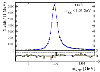
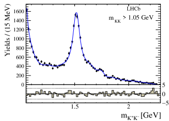
In addition to the expected combinatorial background, studies of the data in sidebands of the spectrum show contributions from approximately () and () decays at greater (less) than 1.05, where the in the former or in the latter is misidentified as a . In order to avoid dealing with correlations between the angular variables and , the contributions from these reflection backgrounds are statistically subtracted by adding to the data simulated events of these decays with negative weights. These weights are chosen so that the distributions of the relevant variables used in the overall fit (see below) describe the background distributions both in normalization and shapes. The simulation uses amplitude models derived from data for [33] and decays [34].
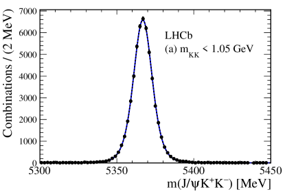
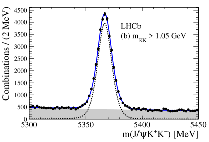
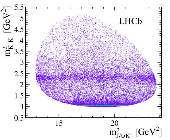
The invariant mass of the selected combinations, separated into samples for below or above 1.05, are shown in Fig. 2, where the expected reflection backgrounds are subtracted using simulation. The combinatorial background is modelled with an exponential function and the signal shape is parameterized by a double-sided Hypatia function [35], where the signal radiative tail parameters are fixed to values obtained from simulation. In total, and signal candidates are found for the low and high intervals, respectively. Figure 3 shows the Dalitz plot distribution of versus for candidates within 15 of the mass peak. Clear resonant contributions from and mesons are seen, but no exotic resonance is observed.
5 Detector resolution and efficiency
The resolution on the decay time is determined with the same method as described in Ref. [7] by using a large sample of prompt combinations produced directly in the interactions. These events are selected using decays via a prescaled trigger that does not impose any requirements on the separation of the from the PV. The candidates are combined with two oppositely charged tracks that are identified as kaons, using a similar selection as for the signal decay, without a decay-time requirement. The resolution function, , where is the true decay time, is a sum of three Gaussian functions with a common mean, and separate widths. To implement the resolution model each of the three widths are given by , where is scale factor for the th Gaussian, is an estimated per-candidate decay-time error and is a constant parameter. The parameters of the resolution model are determined by using a maximum likelihood fit to the unbinned decay time and distributions of the prompt combinations, using a function to represent the prompt component summed with two exponential functions for long-lived backgrounds; these are convolved with the resolution function. Taking into account the distribution of the signal, the average effective resolution is found to be .
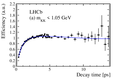
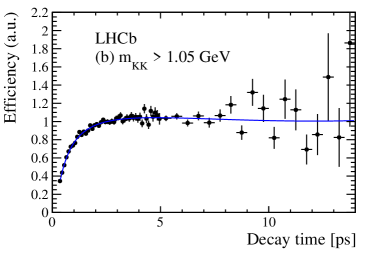
The reconstruction efficiency is not constant as a function of decay time due to displacement requirements made on the candidates in the trigger and offline selections. The efficiency is determined using the control channel , with , which is known to have a purely exponential decay-time distribution with [23]. The selection efficiency is calculated as
| (3) |
where is the efficiency of the control channel and is the ratio of efficiencies of the simulated signal and control mode after the full trigger and selection chain has been applied. This correction accounts for the small differences in the kinematics between the signal and control mode. The details of the method are explained in Ref. [8]. The decay-time efficiencies for the two intervals are shown in Fig. 4.
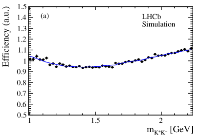
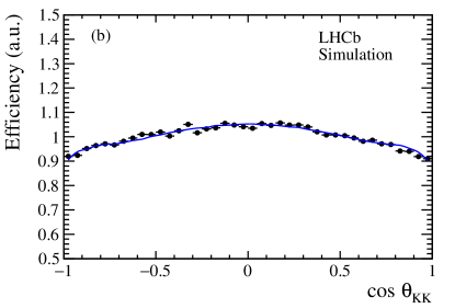
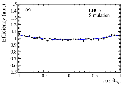
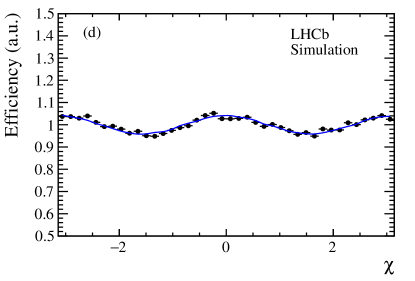
The efficiency as a function of the helicity angles and the invariant mass is not uniform due to the forward geometry of the LHCb detector and the requirements imposed on the final-state particle momenta. The four-dimensional efficiency, , is determined using simulated events that are subjected to the same trigger and selection criteria as the data.
The efficiency is parameterized by
| (4) |
where and are Legendre polynomials, are spherical harmonics, and and are the minimum and maximum allowed values for , respectively. The are complex functions. To ensure that the efficiency function is real, we set . The values of are determined by summing over the fully simulated phase-space events
| (5) |
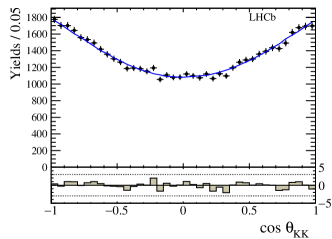
where the weights account for corrections of PID and tracking efficiencies, and is the value of the phase-space probability density for event with being the momentum of either of the two hadrons in the dihadron rest frame and the momentum of the in the rest frame. This approach allows the description of multidimensional correlations without assuming factorization. In practice, the sum is over a finite number of terms (, , , ) and only coefficients with a statistical significance larger than three standard deviations from zero are retained. The number of events in the simulated signal sample is about 20 times of that observed in data. Since a symmetric and efficiency is used, and must be even numbers. Projections of the efficiency integrated over other variables are shown in Fig. 5. The modelling functions describe well the simulated data. Since is not used as a variable in the selection for the two hadrons, the efficiency is quite uniform over all the four variables varying only by about %. (A dedicated simulation of decays is used to determine the efficiency in the region of , in order to have a large enough sample for an accurate determination.)
6 Flavour tagging
The candidate flavour at production is determined using two independent classes of flavour-tagging algorithms, the opposite-side (OS) tagger [36] and the same-side kaon (SSK) tagger [37], which exploit specific features of the production of quark pairs in collisions, and their subsequent hadronisation. Each tagging algorithm provides a tag decision and a mistag probability. The tag decision, , is , , or , if the signal meson is tagged as , , or is untagged, respectively. The fraction of candidates in the sample with a nonzero tagging decision gives the efficiency of the tagger, . The mistag probability, , is estimated event by event, and represents the probability that the algorithm assigns a wrong tag decision to the candidate; it is calibrated using data samples of several flavour-specific , , and [37] decays to obtain the corrected mistag probability, , for an initial meson, and separately obtain for an initial meson. A linear relationship between and ( ) [-.7ex] is used for the calibration. When candidates are tagged by both the OS and the SSK algorithms, a combined tag decision and a wrong-tag probability are given by the algorithm defined in Ref. [36] and extended to include SSK tags. This combined algorithm is implemented in the overall fit. The effective tagging power is given by and for the combined taggers in the signal sample is . Whenever two uncertainties are quoted in this paper, the first is statistical and the second is systematic.
7 Resonance contributions
The entire mass spectrum is fitted by including the resonance contributions previously found in the time-integrated amplitude analysis using 1 of integrated luminosity [14], except for the unconfirmed state. They are shown in Table 1 and are described by Breit-Wigner amplitudes. The S-wave amplitude is described in a model-independent way, making no assumptions about its meson composition, or about the form of any S-wave nonresonant terms. Explicitly, two real parameters and are introduced to define the total S-wave amplitude at each of a set of invariant mass values . Third-order spline interpolations are used to define and between these points of . The and values are treated as model-independent parameters, and are determined by a fit to the data. In total knots are chosen at . The S-wave amplitude is proportional to momentum [16]; at the last point since , the amplitude is zero [16].
| Resonance | Mass (MeV) | Width (MeV) | Source |
|---|---|---|---|
| PDG [23] | |||
| PDG [23] | |||
| Varied in fits | |||
| Belle [38] | |||
| Belle [39] | |||
| Belle [39] | |||
To describe the dependence for each resonance , the formula of Eq. (18) in Ref. [16] is modified by changing to , where is the momentum of either of the two hadrons in the dihadron rest frame, is the mass of resonance , and the orbital angular momentum in the decay, and thus corresponds to the resonance’s spin. This change modifies the lineshape of resonances with spin greater than zero. The original formula followed the convention from the Belle collaboration [40] and was used in two LHCb publications [14, 3], while the new one follows the convention of PDG/EvtGen, and was used in analyzing decays [34].
8 Maximum likelihood fit
The physics parameters are determined from a weighted maximum likelihood fit of a signal-only probability density function (PDF) to the five-dimensional distributions of and decay time, and helicity angles. The negative log-likelihood function to be minimized is given by
| (6) |
where runs over all event candidates, is the sWeight computed using as the discriminating variable [41, *Xie:2009rka] and the factor is a constant factor accounting for the effect of the background subtraction on the statistical uncertainty. The sWeights are determined by separate fits in four bins for the event candidates. The PDF is given by , where is
| (7) |
with
| (8) |
where is the true decay time, ( ) [-.7ex] is defined in Eqs. (2) and (2), and is the LHCb measured production asymmetry of and mesons [43, *Aaij:2017mso].
To obtain a measurement that is independent of the previous publication that used mainly decays [7], two different sets of fit parameters (, , , )L,H are used to account for the low () and high () regions. Simulated pseudoexperiments show that this configuration removes the correlation for these parameters between the two regions. A simultaneous fit to the two samples is performed by constructing the log-likelihood as the sum of that computed from the and events. The shared parameters are all the resonance amplitudes and phases, and , which is freely varied in the fit. In the nominal fit configuration, violation is assumed to be the same for all the transversity states. In total 69 free parameters are used in the nominal fit.
The decay observables resulting from the fit for the high region are listed in Table 2. The measurements for these parameters and in the region are consistent with the reported values in Ref. [7] within 1.4, taking into account the overlap between the two samples used. In addition, good agreement is also found for the S-wave phase. The fit gives from the full region, which is consistent with the most precise measurement from LHCb in decays [45]. The value of is consistent with unity, thus giving no indication of any direct violation in the decay amplitude.
| Parameter | Value |
|---|---|
| [ ] | |
| [ ] | |
| [ mrad ] | |
While a complete description of the decay is given in terms of the fitted amplitudes and phases, knowledge of the contribution of each component can be summarized by the fit fraction, , defined as the integral of the squared amplitude of each resonance over the phase space divided by the integral of the entire signal function over the same area, as given in Eq. 9
| (9) |
The sum of the fit fractions is not necessarily unity due to the potential presence of interference between two resonances.
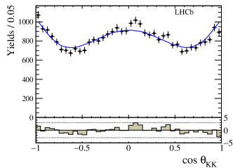
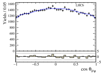
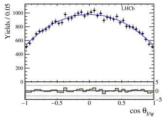
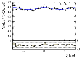
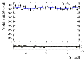
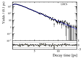
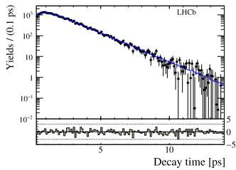
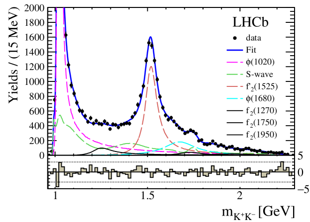
The fit fractions are reported in Table 3 and resonance phases in Table 4. Fit projections are shown in Fig. 6 for the region and above. The fit reproduces the data in each of the projected variables. Each contributing component is shown in Fig. 7 as a function of . To check the fit quality in the high region, tests are performed. For and , =1401 for 1125 bins (25 for , 5 for , 3 for and 3 for ); for the two variables and , =380 for 310 bins. The fit describes the data well. Note, adding the into the fit improves the by 0.4 with an additional 6 degrees of freedom, showing that this state is not observed.
| Component | Fit fraction (%) | Transversity fraction (%) | ||
|---|---|---|---|---|
| S-wave | ||||
| States | Phase difference (∘) | |
|---|---|---|
As a check a fit is performed allowing independent sets of -violating parameters : three sets for the three corresponding transversity states, one for the S-wave, one common to all three transversity states of the , one for the , one for the , and one for the combination of the two high-mass and resonances. In total, eight sets of -violating parameters are used instead of two sets in the nominal fit. The value is improved by 16 units with 12 additional parameters compared to the nominal fit, corresponding to the fact that all states have consistent violation within 1.3 . All values of are consistent with unity and differences of the longitudinal component are consistent with zero, showing no dependence of violation for the different states.
9 Systematic uncertainties
The systematic uncertainties are summarized for the physics parameters in Table 5 and for the fit fractions in Table 6. They are small compared to the statistical ones for the -violating parameters. Generally, the largest contribution results from the resonance fit model. The fit model uncertainties are determined by doubling the number of S-wave knots in the high region, allowing the centrifugal barrier factors, of nominal value for resonances and for the meson [34], to vary within 0.5–2 times of these values [46]. Additional systematic uncertainties are evaluated by increasing the orbital angular momentum between the and the system from the lowest allowed one, which is taken as the nominal value, and varying the masses and widths of contributing resonances by their uncertainties. The largest variation among those changes is assigned as the systematic uncertainty for resonance modelling. The effect of using the in the fit, rather than following the Belle approach using is evaluated by redoing the fit. This change worsens the by more than 100 units, which clearly shows the variation doesn’t give a good fit; as a consequence, no systematic uncertainty is assessed. Differences resulting from the two conventions are comparable to the quoted modelling uncertainty for the -violating parameters, but generally are larger than the quoted systematic uncertainties for the fit fractions of nonscalar resonances.
| Source | ||||||
| [ ] | [ ] | [ ] | [ ] | [rad] | ||
| Resonance modelling | ||||||
| Efficiency (, ) | ||||||
| Efficiency | ||||||
| resolution | ||||||
| Fit bias | 5.0 | 1.1 | - | - | - | - |
| Tagging | ||||||
| Background | ||||||
| - | - | - | - | - | ||
| Total syst. | ||||||
| Stat. |
| Source | S-wave | ||||||
|---|---|---|---|---|---|---|---|
| Res. modelling | |||||||
| Efficiency | |||||||
| Background | |||||||
| Total syst. | |||||||
| Statistical |
The sources of uncertainty for the modelling of the efficiency variation of the three angles and include the statistical uncertainty from simulation, and the efficiency correction due to the differences in kinematic distributions between data and simulation for decays. The former is estimated by repeating the fit to the data 100 times. In each fit, the efficiency parameters are resampled according to the corresponding covariance matrix determined from simulation. For the latter, the efficiency used by the nominal fit is obtained by weighting the distributions of and of the kaon pair and meson to match the data. Such weighting is removed to assign the corresponding systematic uncertainty.
The uncertainties due to the lifetime and decay time efficiency determination are estimated. Each source is evaluated by adding to the nominal fit an external correlated multidimensional Gaussian constraint, either given by the fit to the sample with varying [23], or given by the fit to simulation for the decay time efficiency correction, i.e. in Eq. (3). A systematic uncertainty is given by the difference in quadrature of the statistical uncertainties for each physics parameter between the nominal fit and the alternative fit with each of these constraints. The uncertainties due to the decay time acceptance are found to be negligible for the fit fraction results.
The sample of prompt mesons combined with two kaon candidates is used to calibrate the per-candidate decay-time error. This method is validated by simulation. Since the detached selection, pointing angle and BDTG requirements cannot be applied to the calibration sample, the simulations show that the calibration overestimates the resolution for decays after final selection by about 4.5%. Therefore, a 5% variation of the widths, and the uncertainty of the mean value are used to estimate uncertainty of the time resolution modelling. The average angular resolution is 6 mrad for all three decay angles. This is small enough to have only negligible effects on the analysis.
A large number of pseudoexperiments is used to validate the fitter and check potential biases in the fit outputs. Biases on and , of their statistical uncertainties, are taken as systematic uncertainties. Calibration parameters of the flavour-tagging algorithm and the – production asymmetry [43] are fixed. The systematic uncertainties due to the calibration of the tagging parameters or the value of are given by the difference in quadrature between the statistical uncertainty for each physics parameter between the nominal fit and an alternative fit where the tagging parameters or are Gaussian-constrained by the corresponding uncertainties. Background sources are tested by varying the decay-time acceptance of the injected reflection backgrounds, changing these background yields by 5%, and also varying the lifetime.
To evaluate the uncertainty of the sPlot method that requires the fit observables being uncorrelated with the variable used to obtain the sWeights, two variations are performed to obtain new sWeights, and the fit is repeated. The first consists of changing the number of bins. In the nominal fit, the sWeights are determined by separate fits in four bins for the event candidates, as significant variations of signal invariant mass resolution are seen as a function of the variable. In another variation of the analysis starting with the nominal number of bins the decay time dependence is explored, since the combinatorial background may have a possible variation as a function of . Here the decay time is further divided into three intervals. The larger change on the physics parameter of interest is taken as a systematic uncertainty.
About 0.8% of the signal sample is expected from the decays of mesons [47]. Neglecting the contribution in the nominal fit leads to a negligible bias of 0.0005 for [7]. The correlation matrix with both statistical and systematic uncertainties is shown in Table 7.
10 Conclusions
We have studied and decays into the final state using a time-dependent amplitude analysis. In the region we determine
Many resonances and a S-wave structure have been found. Besides the meson these include the , the , the , the , and the mesons. The presence of the resonance is not confirmed. The measured -violating parameters of the individual resonances are consistent. The mass and width are determined as and , respectively. The fit fractions of the resonances in are also determined, and shown in Table 3. These results supersede our previous measurements [14].
The combination with the previous results from decays in the region [7] gives
The two results are consistent within . A further combination is performed by including the and measurements from and decays into [8], which results in mrad and , where and are unchanged. The correlation matrix is shown in Table 8. The measurement of the -violating phase is in agreement with the SM prediction mrad [1]. These new combined results supersede our combination reported in Ref. [7].
Acknowledgements
We express our gratitude to our colleagues in the CERN accelerator departments for the excellent performance of the LHC. We thank the technical and administrative staff at the LHCb institutes. We acknowledge support from CERN and from the national agencies: CAPES, CNPq, FAPERJ and FINEP (Brazil); MOST and NSFC (China); CNRS/IN2P3 (France); BMBF, DFG and MPG (Germany); INFN (Italy); NWO (The Netherlands); MNiSW and NCN (Poland); MEN/IFA (Romania); MinES and FASO (Russia); MinECo (Spain); SNSF and SER (Switzerland); NASU (Ukraine); STFC (United Kingdom); NSF (USA). We acknowledge the computing resources that are provided by CERN, IN2P3 (France), KIT and DESY (Germany), INFN (Italy), SURF (The Netherlands), PIC (Spain), GridPP (United Kingdom), RRCKI and Yandex LLC (Russia), CSCS (Switzerland), IFIN-HH (Romania), CBPF (Brazil), PL-GRID (Poland) and OSC (USA). We are indebted to the communities behind the multiple open source software packages on which we depend. Individual groups or members have received support from AvH Foundation (Germany), EPLANET, Marie Skłodowska-Curie Actions and ERC (European Union), Conseil Général de Haute-Savoie, Labex ENIGMASS and OCEVU, Région Auvergne (France), RFBR and Yandex LLC (Russia), GVA, XuntaGal and GENCAT (Spain), Herchel Smith Fund, The Royal Society, Royal Commission for the Exhibition of 1851 and the Leverhulme Trust (United Kingdom).
Appendix
Appendix A Angular moments
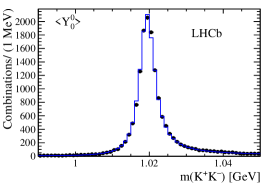
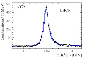
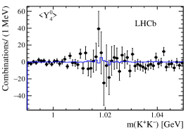
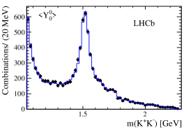
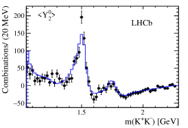
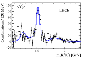
We define the moments , as the efficiency-corrected and background-subtracted invariant mass distributions, weighted by the th spherical harmonic functions of the cosine of the helicity angle . The moment distributions provide an additional way of visualizing the presence of different resonances and their interferences, similar to a partial wave analysis. Figures 8 and 9 show the distributions of the even angular moments for the events around MeV of mass peak and those above the , respectively. The general interpretation of the even moments is that is the efficiency-corrected and background-subtracted event distribution, reflects the sum of P-wave, D-wave and the interference of S-wave and D-wave amplitudes, and the D-wave. The average of and decays cancels the interference terms that involve P-wave amplitudes. This causes the odd moments to sum to zero.
The fit results reproduce the moment distributions relatively well. For the region near the , the -values are 3%, 3%, 48% for the =0, 2, 4 moments, respectively. For the high mass region, the -values are 37%, 0.2% 0.5% for the =0, 2, 4 moments, respectively.
References
- [1] J. Charles et al., Current status of the Standard Model CKM fit and constraints on new physics, Phys. Rev. D91 (2015) 073007, arXiv:1501.05013
- [2] R. Fleischer, Theoretical prospects for B physics, PoS FPCP2015 (2015) 002, arXiv:1509.00601
- [3] LHCb collaboration, R. Aaij et al., Measurement of the -violating phase in decays and limits on penguin effects, Phys. Lett. B742 (2015) 38, arXiv:1411.1634
- [4] LHCb collaboration, R. Aaij et al., Measurement of violation parameters and polarisation fractions in decays, JHEP 11 (2015) 082, arXiv:1509.00400
- [5] D0 collaboration, V. M. Abazov et al., Measurement of the -violating phase using the flavor-tagged decay in 8 fb-1 of collisions, Phys. Rev. D85 (2012) 032006, arXiv:1109.3166
- [6] CDF collaboration, T. Aaltonen et al., Measurement of the bottom-strange meson mixing phase in the full CDF data set, Phys. Rev. Lett. 109 (2012) 171802, arXiv:1208.2967
- [7] LHCb collaboration, R. Aaij et al., Precision measurement of violation in decays, Phys. Rev. Lett. 114 (2015) 041801, arXiv:1411.3104
- [8] LHCb collaboration, R. Aaij et al., Measurement of the -violating phase in decays, Phys. Lett. B736 (2014) 186, arXiv:1405.4140
- [9] CMS collaboration, V. Khachatryan et al., Measurement of the -violating weak phase and the decay width difference using the decay channel in pp collisions at 8 TeV, Phys. Lett. B757 (2016) 97, arXiv:1507.07527
- [10] ATLAS collaboration, G. Aad et al., Measurement of the -violating phase and the meson decay width difference with decays in ATLAS, JHEP 08 (2016) 147, arXiv:1601.03297
- [11] LHCb collaboration, R. Aaij et al., Measurement of the -violating phase in decays, Phys. Rev. Lett. 113 (2014) 211801, arXiv:1409.4619
- [12] LHCb collaboration, R. Aaij et al., First study of the CP-violating phase and decay-width difference in decays, Phys. Lett. B762 (2016) 253, arXiv:1608.04855
- [13] Heavy Flavor Averaging Group, Y. Amhis et al., Averages of -hadron, -hadron, and -lepton properties as of summer 2016, arXiv:1612.07233, updated results and plots available at http://www.slac.stanford.edu/xorg/hfag/
- [14] LHCb collaboration, R. Aaij et al., Amplitude analysis and branching fraction measurement of , Phys. Rev. D87 (2013) 072004, arXiv:1302.1213
- [15] LHCb collaboration, R. Aaij et al., Observation of in final states, Phys. Rev. Lett. 108 (2012) 151801, arXiv:1112.4695
- [16] L. Zhang and S. Stone, Time-dependent Dalitz-plot formalism for , Phys. Lett. B719 (2013) 383, arXiv:1212.6434
- [17] A. S. Dighe, I. Dunietz, H. J. Lipkin, and J. L. Rosner, Angular distributions and lifetime differences in decays, Phys. Lett. B369 (1996) 144, arXiv:hep-ph/9511363
- [18] I. I. Y. Bigi and A. I. Sanda, CP violation, Camb. Monogr. Part. Phys. Nucl. Phys. Cosmol. 9 (2000) 1
- [19] LHCb collaboration, R. Aaij et al., Measurement of violation and the meson decay width difference with and decays, Phys. Rev. D87 (2013) 112010, arXiv:1304.2600
- [20] LHCb collaboration, R. Aaij et al., Measurement of the asymmetry in mixing, Phys. Rev. Lett. 117 (2016) 061803, arXiv:1605.09768
- [21] LHCb collaboration, A. A. Alves Jr. et al., The LHCb detector at the LHC, JINST 3 (2008) S08005
- [22] LHCb collaboration, R. Aaij et al., LHCb detector performance, Int. J. Mod. Phys. A30 (2015) 1530022, arXiv:1412.6352
- [23] Particle Data Group, C. Patrignani et al., Review of particle physics, Chin. Phys. C40 (2016) 100001
- [24] T. Sjöstrand, S. Mrenna, and P. Skands, PYTHIA 6.4 physics and manual, JHEP 05 (2006) 026, arXiv:hep-ph/0603175
- [25] T. Sjöstrand, S. Mrenna, and P. Skands, A brief introduction to PYTHIA 8.1, Comput. Phys. Commun. 178 (2008) 852, arXiv:0710.3820
- [26] D. J. Lange, The EvtGen particle decay simulation package, Nucl. Instrum. Meth. A462 (2001) 152
- [27] P. Golonka and Z. Was, PHOTOS Monte Carlo: A precision tool for QED corrections in and decays, Eur. Phys. J. C45 (2006) 97, arXiv:hep-ph/0506026
- [28] Geant4 collaboration, J. Allison et al., Geant4 developments and applications, IEEE Trans. Nucl. Sci. 53 (2006) 270
- [29] Geant4 collaboration, S. Agostinelli et al., Geant4: A simulation toolkit, Nucl. Instrum. Meth. A506 (2003) 250
- [30] M. Clemencic et al., The LHCb simulation application, Gauss: Design, evolution and experience, J. Phys. Conf. Ser. 331 (2011) 032023
- [31] L. Breiman, J. H. Friedman, R. A. Olshen, and C. J. Stone, Classification and regression trees, Wadsworth international group, Belmont, California, USA, 1984
- [32] M. Adinolfi et al., Performance of the LHCb RICH detector at the LHC, Eur. Phys. J. C73 (2013) 2431, arXiv:1211.6759
- [33] Belle collaboration, K. Chilikin et al., Observation of a new charged charmoniumlike state in decays, Phys. Rev. D90 (2014) 112009, arXiv:1408.6457
- [34] LHCb collaboration, R. Aaij et al., Observation of resonances consistent with pentaquark states in decays, Phys. Rev. Lett. 115 (2015) 072001, arXiv:1507.03414
- [35] D. Martínez Santos and F. Dupertuis, Mass distributions marginalized over per-event errors, Nucl. Instrum. Meth. A764 (2014) 150, arXiv:1312.5000
- [36] LHCb collaboration, R. Aaij et al., Opposite-side flavour tagging of mesons at the LHCb experiment, Eur. Phys. J. C72 (2012) 2022, arXiv:1202.4979
- [37] LHCb collaboration, R. Aaij et al., Neural-network-based same side kaon tagging algorithm calibrated with and decays, JINST 11 (2016) P05010, arXiv:1602.07252
- [38] Belle collaboration, C. P. Shen et al., Observation of the and the in , Phys. Rev. D80 (2009) 031101, arXiv:0808.0006
- [39] Belle collaboration, K. Abe et al., Measurement of production in two-photon collisions in the resonant mass region, Eur. Phys. J. C32 (2003) 323, arXiv:hep-ex/0309077
- [40] Belle collaboration, R. Mizuk et al., Observation of two resonance-like structures in the mass distribution in exclusive decays, Phys. Rev. D78 (2008) 072004, arXiv:0806.4098
- [41] M. Pivk and F. R. Le Diberder, sPlot: A statistical tool to unfold data distributions, Nucl. Instrum. Meth. A555 (2005) 356, arXiv:physics/0402083
- [42] Y. Xie, sFit: a method for background subtraction in maximum likelihood fit, arXiv:0905.0724
- [43] LHCb collaboration, R. Aaij et al., Measurement of the – and – production asymmetries in collisions at , Phys. Lett. B739 (2014) 218, arXiv:1408.0275
- [44] LHCb, R. Aaij et al., Measurement of , , and production asymmetries in 7 and 8 TeV proton-proton collisions, arXiv:1703.08464
- [45] LHCb collaboration, R. Aaij et al., Precision measurement of the – oscillation frequency in the decay , New J. Phys. 15 (2013) 053021, arXiv:1304.4741
- [46] F. Von Hippel and C. Quigg, Centrifugal-barrier effects in resonance partial decay widths, shapes, and production amplitudes, Phys. Rev. D5 (1972) 624
- [47] LHCb collaboration, R. Aaij et al., Observation of the decay , Phys. Rev. Lett. 111 (2013) 181801, arXiv:1308.4544
LHCb collaboration
R. Aaij40,
B. Adeva39,
M. Adinolfi48,
Z. Ajaltouni5,
S. Akar59,
J. Albrecht10,
F. Alessio40,
M. Alexander53,
S. Ali43,
G. Alkhazov31,
P. Alvarez Cartelle55,
A.A. Alves Jr59,
S. Amato2,
S. Amerio23,
Y. Amhis7,
L. An3,
L. Anderlini18,
G. Andreassi41,
M. Andreotti17,g,
J.E. Andrews60,
R.B. Appleby56,
F. Archilli43,
P. d’Argent12,
J. Arnau Romeu6,
A. Artamonov37,
M. Artuso61,
E. Aslanides6,
G. Auriemma26,
M. Baalouch5,
I. Babuschkin56,
S. Bachmann12,
J.J. Back50,
A. Badalov38,
C. Baesso62,
S. Baker55,
V. Balagura7,c,
W. Baldini17,
A. Baranov35,
R.J. Barlow56,
C. Barschel40,
S. Barsuk7,
W. Barter56,
F. Baryshnikov32,
M. Baszczyk27,l,
V. Batozskaya29,
B. Batsukh61,
V. Battista41,
A. Bay41,
L. Beaucourt4,
J. Beddow53,
F. Bedeschi24,
I. Bediaga1,
A. Beiter61,
L.J. Bel43,
V. Bellee41,
N. Belloli21,i,
K. Belous37,
I. Belyaev32,
E. Ben-Haim8,
G. Bencivenni19,
S. Benson43,
S. Beranek9,
A. Berezhnoy33,
R. Bernet42,
A. Bertolin23,
C. Betancourt42,
F. Betti15,
M.-O. Bettler40,
M. van Beuzekom43,
Ia. Bezshyiko42,
S. Bifani47,
P. Billoir8,
A. Birnkraut10,
A. Bitadze56,
A. Bizzeti18,u,
T. Blake50,
F. Blanc41,
J. Blouw11,†,
S. Blusk61,
V. Bocci26,
T. Boettcher58,
A. Bondar36,w,
N. Bondar31,
W. Bonivento16,
I. Bordyuzhin32,
A. Borgheresi21,i,
S. Borghi56,
M. Borisyak35,
M. Borsato39,
F. Bossu7,
M. Boubdir9,
T.J.V. Bowcock54,
E. Bowen42,
C. Bozzi17,40,
S. Braun12,
T. Britton61,
J. Brodzicka56,
E. Buchanan48,
C. Burr56,
A. Bursche2,
J. Buytaert40,
S. Cadeddu16,
R. Calabrese17,g,
M. Calvi21,i,
M. Calvo Gomez38,m,
A. Camboni38,
P. Campana19,
D.H. Campora Perez40,
L. Capriotti56,
A. Carbone15,e,
G. Carboni25,j,
R. Cardinale20,h,
A. Cardini16,
P. Carniti21,i,
L. Carson52,
K. Carvalho Akiba2,
G. Casse54,
L. Cassina21,i,
L. Castillo Garcia41,
M. Cattaneo40,
G. Cavallero20,
R. Cenci24,t,
D. Chamont7,
M. Charles8,
Ph. Charpentier40,
G. Chatzikonstantinidis47,
M. Chefdeville4,
S. Chen56,
S.F. Cheung57,
V. Chobanova39,
M. Chrzaszcz42,27,
A. Chubykin31,
X. Cid Vidal39,
G. Ciezarek43,
P.E.L. Clarke52,
M. Clemencic40,
H.V. Cliff49,
J. Closier40,
V. Coco59,
J. Cogan6,
E. Cogneras5,
V. Cogoni16,f,
L. Cojocariu30,
P. Collins40,
A. Comerma-Montells12,
A. Contu40,
A. Cook48,
G. Coombs40,
S. Coquereau38,
G. Corti40,
M. Corvo17,g,
C.M. Costa Sobral50,
B. Couturier40,
G.A. Cowan52,
D.C. Craik52,
A. Crocombe50,
M. Cruz Torres62,
S. Cunliffe55,
R. Currie52,
C. D’Ambrosio40,
F. Da Cunha Marinho2,
E. Dall’Occo43,
J. Dalseno48,
A. Davis3,
K. De Bruyn6,
S. De Capua56,
M. De Cian12,
J.M. De Miranda1,
L. De Paula2,
M. De Serio14,d,
P. De Simone19,
C.T. Dean53,
D. Decamp4,
M. Deckenhoff10,
L. Del Buono8,
H.-P. Dembinski11,
M. Demmer10,
A. Dendek28,
D. Derkach35,
O. Deschamps5,
F. Dettori54,
B. Dey22,
A. Di Canto40,
P. Di Nezza19,
H. Dijkstra40,
F. Dordei40,
M. Dorigo41,
A. Dosil Suárez39,
A. Dovbnya45,
K. Dreimanis54,
L. Dufour43,
G. Dujany56,
K. Dungs40,
P. Durante40,
R. Dzhelyadin37,
M. Dziewiecki12,
A. Dziurda40,
A. Dzyuba31,
N. Déléage4,
S. Easo51,
M. Ebert52,
U. Egede55,
V. Egorychev32,
S. Eidelman36,w,
S. Eisenhardt52,
U. Eitschberger10,
R. Ekelhof10,
L. Eklund53,
S. Ely61,
S. Esen12,
H.M. Evans49,
T. Evans57,
A. Falabella15,
N. Farley47,
S. Farry54,
R. Fay54,
D. Fazzini21,i,
D. Ferguson52,
G. Fernandez38,
A. Fernandez Prieto39,
F. Ferrari15,
F. Ferreira Rodrigues2,
M. Ferro-Luzzi40,
S. Filippov34,
R.A. Fini14,
M. Fiore17,g,
M. Fiorini17,g,
M. Firlej28,
C. Fitzpatrick41,
T. Fiutowski28,
F. Fleuret7,b,
K. Fohl40,
M. Fontana16,40,
F. Fontanelli20,h,
D.C. Forshaw61,
R. Forty40,
V. Franco Lima54,
M. Frank40,
C. Frei40,
J. Fu22,q,
W. Funk40,
E. Furfaro25,j,
C. Färber40,
A. Gallas Torreira39,
D. Galli15,e,
S. Gallorini23,
S. Gambetta52,
M. Gandelman2,
P. Gandini57,
Y. Gao3,
L.M. Garcia Martin69,
J. García Pardiñas39,
J. Garra Tico49,
L. Garrido38,
P.J. Garsed49,
D. Gascon38,
C. Gaspar40,
L. Gavardi10,
G. Gazzoni5,
D. Gerick12,
E. Gersabeck12,
M. Gersabeck56,
T. Gershon50,
Ph. Ghez4,
S. Gianì41,
V. Gibson49,
O.G. Girard41,
L. Giubega30,
K. Gizdov52,
V.V. Gligorov8,
D. Golubkov32,
A. Golutvin55,40,
A. Gomes1,a,
I.V. Gorelov33,
C. Gotti21,i,
E. Govorkova43,
R. Graciani Diaz38,
L.A. Granado Cardoso40,
E. Graugés38,
E. Graverini42,
G. Graziani18,
A. Grecu30,
R. Greim9,
P. Griffith16,
L. Grillo21,40,i,
B.R. Gruberg Cazon57,
O. Grünberg67,
E. Gushchin34,
Yu. Guz37,
T. Gys40,
C. Göbel62,
T. Hadavizadeh57,
C. Hadjivasiliou5,
G. Haefeli41,
C. Haen40,
S.C. Haines49,
B. Hamilton60,
X. Han12,
S. Hansmann-Menzemer12,
N. Harnew57,
S.T. Harnew48,
J. Harrison56,
M. Hatch40,
J. He63,
T. Head41,
A. Heister9,
K. Hennessy54,
P. Henrard5,
L. Henry69,
E. van Herwijnen40,
M. Heß67,
A. Hicheur2,
D. Hill57,
C. Hombach56,
P.H. Hopchev41,
Z.-C. Huard59,
W. Hulsbergen43,
T. Humair55,
M. Hushchyn35,
D. Hutchcroft54,
M. Idzik28,
P. Ilten58,
R. Jacobsson40,
J. Jalocha57,
E. Jans43,
A. Jawahery60,
F. Jiang3,
M. John57,
D. Johnson40,
C.R. Jones49,
C. Joram40,
B. Jost40,
N. Jurik57,
S. Kandybei45,
M. Karacson40,
J.M. Kariuki48,
S. Karodia53,
M. Kecke12,
M. Kelsey61,
M. Kenzie49,
T. Ketel44,
E. Khairullin35,
B. Khanji12,
C. Khurewathanakul41,
T. Kirn9,
S. Klaver56,
K. Klimaszewski29,
T. Klimkovich11,
S. Koliiev46,
M. Kolpin12,
I. Komarov41,
R. Kopecna12,
P. Koppenburg43,
A. Kosmyntseva32,
S. Kotriakhova31,
A. Kozachuk33,
M. Kozeiha5,
L. Kravchuk34,
M. Kreps50,
P. Krokovny36,w,
F. Kruse10,
W. Krzemien29,
W. Kucewicz27,l,
M. Kucharczyk27,
V. Kudryavtsev36,w,
A.K. Kuonen41,
K. Kurek29,
T. Kvaratskheliya32,40,
D. Lacarrere40,
G. Lafferty56,
A. Lai16,
G. Lanfranchi19,
C. Langenbruch9,
T. Latham50,
C. Lazzeroni47,
R. Le Gac6,
J. van Leerdam43,
A. Leflat33,40,
J. Lefrançois7,
R. Lefèvre5,
F. Lemaitre40,
E. Lemos Cid39,
O. Leroy6,
T. Lesiak27,
B. Leverington12,
T. Li3,
Y. Li7,
Z. Li61,
T. Likhomanenko35,68,
R. Lindner40,
F. Lionetto42,
X. Liu3,
D. Loh50,
I. Longstaff53,
J.H. Lopes2,
D. Lucchesi23,o,
M. Lucio Martinez39,
H. Luo52,
A. Lupato23,
E. Luppi17,g,
O. Lupton40,
A. Lusiani24,
X. Lyu63,
F. Machefert7,
F. Maciuc30,
O. Maev31,
K. Maguire56,
S. Malde57,
A. Malinin68,
T. Maltsev36,
G. Manca16,f,
G. Mancinelli6,
P. Manning61,
J. Maratas5,v,
J.F. Marchand4,
U. Marconi15,
C. Marin Benito38,
M. Marinangeli41,
P. Marino24,t,
J. Marks12,
G. Martellotti26,
M. Martin6,
M. Martinelli41,
D. Martinez Santos39,
F. Martinez Vidal69,
D. Martins Tostes2,
L.M. Massacrier7,
A. Massafferri1,
R. Matev40,
A. Mathad50,
Z. Mathe40,
C. Matteuzzi21,
A. Mauri42,
E. Maurice7,b,
B. Maurin41,
A. Mazurov47,
M. McCann55,40,
A. McNab56,
R. McNulty13,
B. Meadows59,
F. Meier10,
D. Melnychuk29,
M. Merk43,
A. Merli22,40,q,
E. Michielin23,
D.A. Milanes66,
M.-N. Minard4,
D.S. Mitzel12,
A. Mogini8,
J. Molina Rodriguez1,
I.A. Monroy66,
S. Monteil5,
M. Morandin23,
M.J. Morello24,t,
O. Morgunova68,
J. Moron28,
A.B. Morris52,
R. Mountain61,
F. Muheim52,
M. Mulder43,
M. Mussini15,
D. Müller56,
J. Müller10,
K. Müller42,
V. Müller10,
P. Naik48,
T. Nakada41,
R. Nandakumar51,
A. Nandi57,
I. Nasteva2,
M. Needham52,
N. Neri22,40,
S. Neubert12,
N. Neufeld40,
M. Neuner12,
T.D. Nguyen41,
C. Nguyen-Mau41,n,
S. Nieswand9,
R. Niet10,
N. Nikitin33,
T. Nikodem12,
A. Nogay68,
A. Novoselov37,
D.P. O’Hanlon50,
A. Oblakowska-Mucha28,
V. Obraztsov37,
S. Ogilvy19,
R. Oldeman16,f,
C.J.G. Onderwater70,
A. Ossowska27,
J.M. Otalora Goicochea2,
P. Owen42,
A. Oyanguren69,
P.R. Pais41,
A. Palano14,d,
M. Palutan19,40,
A. Papanestis51,
M. Pappagallo14,d,
L.L. Pappalardo17,g,
C. Pappenheimer59,
W. Parker60,
C. Parkes56,
G. Passaleva18,
A. Pastore14,d,
M. Patel55,
C. Patrignani15,e,
A. Pearce40,
A. Pellegrino43,
G. Penso26,
M. Pepe Altarelli40,
S. Perazzini40,
P. Perret5,
L. Pescatore41,
K. Petridis48,
A. Petrolini20,h,
A. Petrov68,
M. Petruzzo22,q,
E. Picatoste Olloqui38,
B. Pietrzyk4,
M. Pikies27,
D. Pinci26,
A. Pistone20,
A. Piucci12,
V. Placinta30,
S. Playfer52,
M. Plo Casasus39,
T. Poikela40,
F. Polci8,
M. Poli Lener19,
A. Poluektov50,36,
I. Polyakov61,
E. Polycarpo2,
G.J. Pomery48,
S. Ponce40,
A. Popov37,
D. Popov11,40,
B. Popovici30,
S. Poslavskii37,
C. Potterat2,
E. Price48,
J. Prisciandaro39,
C. Prouve48,
V. Pugatch46,
A. Puig Navarro42,
G. Punzi24,p,
C. Qian63,
W. Qian50,
R. Quagliani7,48,
B. Rachwal28,
J.H. Rademacker48,
M. Rama24,
M. Ramos Pernas39,
M.S. Rangel2,
I. Raniuk45,†,
F. Ratnikov35,
G. Raven44,
F. Redi55,
S. Reichert10,
A.C. dos Reis1,
C. Remon Alepuz69,
V. Renaudin7,
S. Ricciardi51,
S. Richards48,
M. Rihl40,
K. Rinnert54,
V. Rives Molina38,
P. Robbe7,
A.B. Rodrigues1,
E. Rodrigues59,
J.A. Rodriguez Lopez66,
P. Rodriguez Perez56,†,
A. Rogozhnikov35,
S. Roiser40,
A. Rollings57,
V. Romanovskiy37,
A. Romero Vidal39,
J.W. Ronayne13,
M. Rotondo19,
M.S. Rudolph61,
T. Ruf40,
P. Ruiz Valls69,
J.J. Saborido Silva39,
E. Sadykhov32,
N. Sagidova31,
B. Saitta16,f,
V. Salustino Guimaraes1,
D. Sanchez Gonzalo38,
C. Sanchez Mayordomo69,
B. Sanmartin Sedes39,
R. Santacesaria26,
C. Santamarina Rios39,
M. Santimaria19,
E. Santovetti25,j,
A. Sarti19,k,
C. Satriano26,s,
A. Satta25,
D.M. Saunders48,
D. Savrina32,33,
S. Schael9,
M. Schellenberg10,
M. Schiller53,
H. Schindler40,
M. Schlupp10,
M. Schmelling11,
T. Schmelzer10,
B. Schmidt40,
O. Schneider41,
A. Schopper40,
H.F. Schreiner59,
K. Schubert10,
M. Schubiger41,
M.-H. Schune7,
R. Schwemmer40,
B. Sciascia19,
A. Sciubba26,k,
A. Semennikov32,
A. Sergi47,
N. Serra42,
J. Serrano6,
L. Sestini23,
P. Seyfert21,
M. Shapkin37,
I. Shapoval45,
Y. Shcheglov31,
T. Shears54,
L. Shekhtman36,w,
V. Shevchenko68,
B.G. Siddi17,40,
R. Silva Coutinho42,
L. Silva de Oliveira2,
G. Simi23,o,
S. Simone14,d,
M. Sirendi49,
N. Skidmore48,
T. Skwarnicki61,
E. Smith55,
I.T. Smith52,
J. Smith49,
M. Smith55,
l. Soares Lavra1,
M.D. Sokoloff59,
F.J.P. Soler53,
B. Souza De Paula2,
B. Spaan10,
P. Spradlin53,
S. Sridharan40,
F. Stagni40,
M. Stahl12,
S. Stahl40,
P. Stefko41,
S. Stefkova55,
O. Steinkamp42,
S. Stemmle12,
O. Stenyakin37,
H. Stevens10,
S. Stoica30,
S. Stone61,
B. Storaci42,
S. Stracka24,p,
M.E. Stramaglia41,
M. Straticiuc30,
U. Straumann42,
L. Sun64,
W. Sutcliffe55,
K. Swientek28,
V. Syropoulos44,
M. Szczekowski29,
T. Szumlak28,
S. T’Jampens4,
A. Tayduganov6,
T. Tekampe10,
G. Tellarini17,g,
F. Teubert40,
E. Thomas40,
J. van Tilburg43,
M.J. Tilley55,
V. Tisserand4,
M. Tobin41,
S. Tolk49,
L. Tomassetti17,g,
D. Tonelli24,
S. Topp-Joergensen57,
F. Toriello61,
R. Tourinho Jadallah Aoude1,
E. Tournefier4,
S. Tourneur41,
K. Trabelsi41,
M. Traill53,
M.T. Tran41,
M. Tresch42,
A. Trisovic40,
A. Tsaregorodtsev6,
P. Tsopelas43,
A. Tully49,
N. Tuning43,
A. Ukleja29,
A. Ustyuzhanin35,
U. Uwer12,
C. Vacca16,f,
V. Vagnoni15,40,
A. Valassi40,
S. Valat40,
G. Valenti15,
R. Vazquez Gomez19,
P. Vazquez Regueiro39,
S. Vecchi17,
M. van Veghel43,
J.J. Velthuis48,
M. Veltri18,r,
G. Veneziano57,
A. Venkateswaran61,
T.A. Verlage9,
M. Vernet5,
M. Vesterinen12,
J.V. Viana Barbosa40,
B. Viaud7,
D. Vieira63,
M. Vieites Diaz39,
H. Viemann67,
X. Vilasis-Cardona38,m,
M. Vitti49,
V. Volkov33,
A. Vollhardt42,
B. Voneki40,
A. Vorobyev31,
V. Vorobyev36,w,
C. Voß9,
J.A. de Vries43,
C. Vázquez Sierra39,
R. Waldi67,
C. Wallace50,
R. Wallace13,
J. Walsh24,
J. Wang61,
D.R. Ward49,
H.M. Wark54,
N.K. Watson47,
D. Websdale55,
A. Weiden42,
M. Whitehead40,
J. Wicht50,
G. Wilkinson57,40,
M. Wilkinson61,
M. Williams40,
M.P. Williams47,
M. Williams58,
T. Williams47,
F.F. Wilson51,
J. Wimberley60,
M.A. Winn7,
J. Wishahi10,
W. Wislicki29,
M. Witek27,
G. Wormser7,
S.A. Wotton49,
K. Wraight53,
K. Wyllie40,
Y. Xie65,
Z. Xing61,
Z. Xu4,
Z. Yang3,
Z. Yang60,
Y. Yao61,
H. Yin65,
J. Yu65,
X. Yuan61,
O. Yushchenko37,
K.A. Zarebski47,
M. Zavertyaev11,c,
L. Zhang3,
Y. Zhang7,
A. Zhelezov12,
Y. Zheng63,
X. Zhu3,
V. Zhukov33,
S. Zucchelli15.
1Centro Brasileiro de Pesquisas Físicas (CBPF), Rio de Janeiro, Brazil
2Universidade Federal do Rio de Janeiro (UFRJ), Rio de Janeiro, Brazil
3Center for High Energy Physics, Tsinghua University, Beijing, China
4LAPP, Université Savoie Mont-Blanc, CNRS/IN2P3, Annecy-Le-Vieux, France
5Clermont Université, Université Blaise Pascal, CNRS/IN2P3, LPC, Clermont-Ferrand, France
6CPPM, Aix-Marseille Université, CNRS/IN2P3, Marseille, France
7LAL, Université Paris-Sud, CNRS/IN2P3, Orsay, France
8LPNHE, Université Pierre et Marie Curie, Université Paris Diderot, CNRS/IN2P3, Paris, France
9I. Physikalisches Institut, RWTH Aachen University, Aachen, Germany
10Fakultät Physik, Technische Universität Dortmund, Dortmund, Germany
11Max-Planck-Institut für Kernphysik (MPIK), Heidelberg, Germany
12Physikalisches Institut, Ruprecht-Karls-Universität Heidelberg, Heidelberg, Germany
13School of Physics, University College Dublin, Dublin, Ireland
14Sezione INFN di Bari, Bari, Italy
15Sezione INFN di Bologna, Bologna, Italy
16Sezione INFN di Cagliari, Cagliari, Italy
17Sezione INFN di Ferrara, Ferrara, Italy
18Sezione INFN di Firenze, Firenze, Italy
19Laboratori Nazionali dell’INFN di Frascati, Frascati, Italy
20Sezione INFN di Genova, Genova, Italy
21Sezione INFN di Milano Bicocca, Milano, Italy
22Sezione INFN di Milano, Milano, Italy
23Sezione INFN di Padova, Padova, Italy
24Sezione INFN di Pisa, Pisa, Italy
25Sezione INFN di Roma Tor Vergata, Roma, Italy
26Sezione INFN di Roma La Sapienza, Roma, Italy
27Henryk Niewodniczanski Institute of Nuclear Physics Polish Academy of Sciences, Kraków, Poland
28AGH - University of Science and Technology, Faculty of Physics and Applied Computer Science, Kraków, Poland
29National Center for Nuclear Research (NCBJ), Warsaw, Poland
30Horia Hulubei National Institute of Physics and Nuclear Engineering, Bucharest-Magurele, Romania
31Petersburg Nuclear Physics Institute (PNPI), Gatchina, Russia
32Institute of Theoretical and Experimental Physics (ITEP), Moscow, Russia
33Institute of Nuclear Physics, Moscow State University (SINP MSU), Moscow, Russia
34Institute for Nuclear Research of the Russian Academy of Sciences (INR RAN), Moscow, Russia
35Yandex School of Data Analysis, Moscow, Russia
36Budker Institute of Nuclear Physics (SB RAS), Novosibirsk, Russia
37Institute for High Energy Physics (IHEP), Protvino, Russia
38ICCUB, Universitat de Barcelona, Barcelona, Spain
39Universidad de Santiago de Compostela, Santiago de Compostela, Spain
40European Organization for Nuclear Research (CERN), Geneva, Switzerland
41Institute of Physics, Ecole Polytechnique Fédérale de Lausanne (EPFL), Lausanne, Switzerland
42Physik-Institut, Universität Zürich, Zürich, Switzerland
43Nikhef National Institute for Subatomic Physics, Amsterdam, The Netherlands
44Nikhef National Institute for Subatomic Physics and VU University Amsterdam, Amsterdam, The Netherlands
45NSC Kharkiv Institute of Physics and Technology (NSC KIPT), Kharkiv, Ukraine
46Institute for Nuclear Research of the National Academy of Sciences (KINR), Kyiv, Ukraine
47University of Birmingham, Birmingham, United Kingdom
48H.H. Wills Physics Laboratory, University of Bristol, Bristol, United Kingdom
49Cavendish Laboratory, University of Cambridge, Cambridge, United Kingdom
50Department of Physics, University of Warwick, Coventry, United Kingdom
51STFC Rutherford Appleton Laboratory, Didcot, United Kingdom
52School of Physics and Astronomy, University of Edinburgh, Edinburgh, United Kingdom
53School of Physics and Astronomy, University of Glasgow, Glasgow, United Kingdom
54Oliver Lodge Laboratory, University of Liverpool, Liverpool, United Kingdom
55Imperial College London, London, United Kingdom
56School of Physics and Astronomy, University of Manchester, Manchester, United Kingdom
57Department of Physics, University of Oxford, Oxford, United Kingdom
58Massachusetts Institute of Technology, Cambridge, MA, United States
59University of Cincinnati, Cincinnati, OH, United States
60University of Maryland, College Park, MD, United States
61Syracuse University, Syracuse, NY, United States
62Pontifícia Universidade Católica do Rio de Janeiro (PUC-Rio), Rio de Janeiro, Brazil, associated to 2
63University of Chinese Academy of Sciences, Beijing, China, associated to 3
64School of Physics and Technology, Wuhan University, Wuhan, China, associated to 3
65Institute of Particle Physics, Central China Normal University, Wuhan, Hubei, China, associated to 3
66Departamento de Fisica , Universidad Nacional de Colombia, Bogota, Colombia, associated to 8
67Institut für Physik, Universität Rostock, Rostock, Germany, associated to 12
68National Research Centre Kurchatov Institute, Moscow, Russia, associated to 32
69Instituto de Fisica Corpuscular, Centro Mixto Universidad de Valencia - CSIC, Valencia, Spain, associated to 38
70Van Swinderen Institute, University of Groningen, Groningen, The Netherlands, associated to 43
aUniversidade Federal do Triângulo Mineiro (UFTM), Uberaba-MG, Brazil
bLaboratoire Leprince-Ringuet, Palaiseau, France
cP.N. Lebedev Physical Institute, Russian Academy of Science (LPI RAS), Moscow, Russia
dUniversità di Bari, Bari, Italy
eUniversità di Bologna, Bologna, Italy
fUniversità di Cagliari, Cagliari, Italy
gUniversità di Ferrara, Ferrara, Italy
hUniversità di Genova, Genova, Italy
iUniversità di Milano Bicocca, Milano, Italy
jUniversità di Roma Tor Vergata, Roma, Italy
kUniversità di Roma La Sapienza, Roma, Italy
lAGH - University of Science and Technology, Faculty of Computer Science, Electronics and Telecommunications, Kraków, Poland
mLIFAELS, La Salle, Universitat Ramon Llull, Barcelona, Spain
nHanoi University of Science, Hanoi, Viet Nam
oUniversità di Padova, Padova, Italy
pUniversità di Pisa, Pisa, Italy
qUniversità degli Studi di Milano, Milano, Italy
rUniversità di Urbino, Urbino, Italy
sUniversità della Basilicata, Potenza, Italy
tScuola Normale Superiore, Pisa, Italy
uUniversità di Modena e Reggio Emilia, Modena, Italy
vIligan Institute of Technology (IIT), Iligan, Philippines
wNovosibirsk State University, Novosibirsk, Russia
†Deceased