Renormalization group procedure for potential $-g/r^{2}$

Abstract

Schrödinger equation with potential $-g/r^{2}$ exhibits a limit cycle, described in the literature in a broad range of contexts using various regularizations of the singularity at $r=0$. Instead, we use the renormalization group transformation based on Gaussian elimination, from the Hamiltonian eigenvalue problem. of high momentum modes above a finite, floating cutoff scale. The procedure identifies a richer structure than the one we found in the literature. Namely, it directly yields an equation that determines the renormalized Hamiltonians as functions of the floating cutoff: solutions to this equation exhibit, in addition to the limit-cycle, also the asymptotic-freedom, triviality, and fixed-point behaviors, the latter in vicinity of infinitely many separate pairs of fixed points in different partial waves for different values of $g$.

1 Introduction

Eigenvalue problem for the one-particle Hamiltonian

$$H=\frac{\vec{p}\,^{2}}{2m}-\frac{g}{\vec{r}\,^{2}}\ ,$$ (1)

provides a well-known example of a singular Schrödinger equation. For positive and sufficiently large coupling constant $g$, the overwhelmingly attractive potential causes instability, which limits application of Eq. (1) in physics [1].

The situation is changed when one regularizes the potential and introduces corrections on the basis of demanding that predictions for observables do not depend on the regularization. As a result, the corrected interaction exhibits cyclic behavior as a function of the regularization cutoff parameter. The cycle is associated with an infinite set of bound states whose binding energies form a geometric sequence converging on zero [1, 2, 3, 4, 5, 6, 7, 8, 9].

Regularization of potential $-g/r^{2}$ in the position representation is proposed in various ways [5, 2, 3, 10]. For instance, Braaten and Phillips [5] cut off the potential at some small radius and they introduce an additional potential that acts only in a spherical $\delta$-shell of an infinitesimally smaller radius. They solve the resulting $s$-wave eigenvalue problem and find that one can obtain cutoff independent eigenvalues by making the coupling constant in the additional term a log-periodic function of the cutoff radius.

In the momentum representation, the regularization is formulated differently. For example, in the space of $s$-wave states, Hammer and Swingle [6] introduce an ultraviolet cutoff $\Lambda$ that limits the particle momentum from above. They also add a counter potential with a new coupling constant, $H(\Lambda)$. They determine $H(\Lambda)$ as a function of $\Lambda$ by demanding that the bound-state solution with zero binding energy does not depend on $\Lambda$. Knowing the function $H(\Lambda)$, they find a differential equation that it satisfies. In higher partial waves, Long and van Kolck [8] discuss the potential $-g/r^{2}$ with added contact terms, in the spirit of constructing effective theories. They arrive at cutoff-independent solutions for observables by specifying cycling coefficients in front of one contact term per singular partial wave.

The approach quoted above has successfully amended Eq. (1) with examples of regularization and corresponding correction terms that are justified a posteriori. The ultimate justification relies on the fact that different regularizations with different corrections lead to the same results for observables [11, 12].

In this paper, the Hamiltonian of Eq. (1) is handled using the Wilsonian type of renormalization group procedure [13, 14]. It is the same type of procedure that originally produced the concept of a renormalization group limit cycle [15]. Instead of first calculating observables in a regularized theory, guessing an ansatz for the correction term, and subsequently checking if such a theory can give regularization independent results for the observables, we begin by calculating the required counterterm structure in the presence of regularization. This is done using a renormalization group transformation (RGT) of the Hamiltonian itself [13, 14], i.e., prior to seeking solutions for observables. In the process, a family of finite, effective Hamiltonians is obtained, using the calculated counterterm structure. Solutions for observables are sought first in the resulting finite, scale-dependent effective theories that a priori do not depend on regularization.

Our procedure leads to the limit cycle in terms of solutions to a simple renormalization group equation that evolves a Hamiltonian in the sense of Refs. [13, 14]. The procedure also allows us to identify a whole range of renormalization group behaviors, which characterize the Hamiltonian of Eq. (1), in addition to the limit cycle. These other behaviors, to the best of our knowledge, are not fully identified in the literature. Namely, we exhibit behaviors of the asymptotic-freedom, triviality and fixed-point type. The latter has been found before in the case of $s$-waves, using the functional renormalization group technique that revealed a collision of two fixed points at the critical value of the $s$-wave coupling constant [16]. We identify fixed points in all partial waves, including their behavior near the corresponding infinitely many critical values of the coupling constant. These behaviors appear in a pattern of interest for studies of scaling symmetry and its breakdown in complex theories, see below. Hence, the simplicity and familiarity of Eq. (1) are its assets rather than drawbacks. Further simplification is taken advantage of in this paper by carrying out the RGT in the differential steps that are analogous to the discrete ones outlined in [17, 18] on another example of a Hamiltonian with a limit cycle. The issue of dependence of effective theories on the magnitude of eigenvalues they aim to describe, is only briefly explained at the end of the paper.

Effective potentials of type $1/r^{2}$ were successfully employed in three-body dynamics, where a series of bound states generically appears, under the name of Efimov effect [19, 20, 21, 22], whenever in the corresponding two-body dynamics the ratio of effective interaction range to scattering length is very small, ultimately requiring precise treatment when this ratio approaches zero [23]. It is worth pointing out that a potential of the type $1/r^{2}$ appears also in interactions of a point charge with a dipole, causing violation of scaling symmetry [24, 25]. The pattern of breaking scale invariance when the coupling constant $g$ in Eq. (1) increases above a critical value is of special interest in many areas “from molecular to black-hole physics” [26], and in statistical mechanics [27, 28]. In Ref. [10], the analogous pattern is found helpful in discussing theories that exhibit the Berezinsky-Kosterlitz-Thouless phase transition. It is said to have many “parallels in the AdS/CFT correspondence” [29]. Patterns of conformal symmetry breaking, including breaking of scale invariance in Hamiltonians [30], are invoked in light-front holographic description of hadrons [31] and in studies of conformal windows in technicolor gauge theories [32], the latter hoped to help in understanding the origin of the Standard Model [33, 34]. Equation (1) is thus of broad interest as a rich but simple example of scaling-symmetry breaking and dimensional transmutation [35] in the Wilsonian renormalization group procedure for Hamiltonians.

2 Renormalization group transformation

The renormalization group procedure for an incompletely defined Hamiltonian, such as the one in Eq. (1), starts with regularizing it as an operator in a scheme called the “triangle of renormalization” [36]. We introduce a cutoff $\Delta$ and thus define $H_{\Delta}$, from which we evaluate the equivalent effective Hamiltonians $H_{\Lambda}$ with cutoffs $\Lambda\ll\Delta$. The RGT is involved in the process of this evaluation.

In the limit $\Delta\to\infty$, we demand that matrix elements of $H_{\Lambda}$ in the subspace of states limited by finite $\Lambda$ do not depend on $\Delta$. This condition implies a large, if not infinite set of constraints. It allows us to determine the structure of counterterms needed in $H_{\Delta}$, up to finite alterations in their parameters. The computation of counterterms is done in a sequence of successive approximations, which improves the counterterms put in $H_{\Delta}$ until all matrix elements in $H_{\Lambda}$ in the subspace of states limited by $\Lambda$ become independent of $\Delta$. This finite cutoff becomes a running parameter which enables one to identify how the theoretical description of observable phenomena depends on the range of scales of degrees of freedom one uses for constructing solutions of the theory.

Once the counterterms in $H_{\Delta}$ are such that all matrix elements of $H_{\Lambda}$ have well-defined limits for $\Delta/\Lambda\to\infty$, the eigenvalues of $H_{\Lambda}$ cannot depend on $\Delta$. At the same time, eigenvalues of the effective Hamiltonians $H_{\Lambda}$ that are much smaller than $\Lambda$ cannot depend on $\Lambda$, because this cutoff is merely a mathematical boundary between the implicit degrees of freedom above and explicit degrees of freedom below $\Lambda$. Computation of $H_{\Lambda}$ that is equivalent to $H_{\Delta}$ is carried out in a sequence of discrete, or infinitesimal RGTs.

We carry out a sequence of the RGTs in momentum representation. The stationary Schrödinger equation for Hamiltonian of Eq. (1),

$$\frac{\vec{p}^{\ 2}}{2m}\phi(\vec{p})-{g\over 4\pi}\int d^{3}q\ \frac{\phi(\vec{q})}{|\vec{p}-\vec{q}|}=E\phi(\vec{p}).$$ (2)

is written in terms of angular and radial variables, $\phi(\vec{p})=\sum_{lm}\psi_{l}(p)Y_{lm}(\Omega_{p})$, where $p=|\vec{p}\,|$. Taking advantage of rotational symmetry of Eq. (2), one obtains

$$p^{2}\psi_{l}(p)+\int\limits_{0}^{\infty}\!\!dq~{}q^{2}\ V_{l}(p,q)\ \psi_{l}(q)=\mathcal{E}\psi_{l}(p),$$ (3)

where the eigenvalue $\mathcal{E}=2mE$, the potential

$$V_{l}(p,q)=-\frac{\alpha}{2l+1}~{}\left[\frac{\theta(p-q)~{}q\,^{l}}{p\,^{l+1}}+\frac{\theta(q-p)~{}p\,^{l}}{q\,^{l+1}}\right],$$ (4)

the dimensionless coupling constant $\alpha=2mg$ and the symbol $\theta$ denotes the Heaviside step function. Our regulated eigenvalue problem is defined by limiting the range of momenta $p$ and $q$ by a large cutoff parameter $\Delta$.

Elimination of high momentum modes proceeds by infinitesimal steps such as from $\Delta$ to $\Delta-d\Delta$,

$$p^{2}\psi_{l}(p)\!\! + \!\!\int\limits_{0}^{\Delta-d\Delta}\!dq\ q^{2}\ V_{l}(p,q)\ \psi_{l}(q)$$ (5)

$$- \!\frac{\alpha}{2l+1}\,\frac{p\,^{l}}{\Delta^{l-1}}\,\psi_{l}(\Delta)\ d\Delta=\mathcal{E}\ \psi_{l}(p)\ .$$

The value of $\psi_{l}(\Delta)$ is expressed in terms of values of $\psi_{l}(p)$ with $p<\Delta-d\Delta$ by setting $p=\Delta$ in Eq. (5). For eigenvalues $\mathcal{E}$ much smaller than $\Delta^{2}$, and neglecting terms that lead to quantities of order $d\Delta^{2}$ or smaller in Eq. (5), we have

$$\psi_{l}(\Delta)=\frac{\alpha}{(2l+1)\Delta^{2}}\int\limits_{0}^{\Delta-d\Delta}\!dq\ q^{2}\ \frac{q\,^{l}}{\Delta^{l+1}}\ \psi_{l}(q)\>.$$ (6)

Hence, treating $\Delta-d\Delta$ as a new cutoff $\Lambda$, we obtain

$$p^{2}\ \psi_{l}(p)\!\!\!\!\! + \!\!\!\!\!\int\limits_{0}^{\Lambda}\!dq\ q^{2}\left[V_{l}(p,q)+\gamma_{\Lambda}q\,^{l}p\,^{l}\right]\ \psi_{l}(q)$$ (7)

$$= \!\!\!\mathcal{E}\ \psi_{l}(p)\ ,$$

$$\gamma_{\Lambda}\!\!\! = \!\!\!-\frac{\alpha^{2}d\Delta}{(2l+1)^{2}\Delta^{2l+2}}\ .$$ (8)

Further reduction of the cutoff from $\Lambda$ to $\Lambda-d\Lambda$ produces

$$p^{2}\ \psi_{l}(p)\!\!\! + \!\!\!\!\!\!\!\int\limits_{0}^{\Lambda-d\Lambda}\!dq\ q^{2}\left[V_{l}(p,q)+\gamma_{\Lambda-d\Lambda}q\,^{l}p\,^{l}\right]\psi_{l}(q)$$ (9)

$$= \!\!\mathcal{E}\ \psi_{l}(p)\ ,$$

where

$$\gamma_{\Lambda-d\Lambda}=\gamma_{\Lambda}-\left[\gamma_{\Lambda}\Lambda^{l}-\frac{\alpha}{(2l+1)\Lambda^{l+1}}\right]^{2}d\Lambda\ .$$ (10)

Now no new potential term appears. Only the coupling constant $\gamma_{\Lambda}$ changes to $\gamma_{\Lambda-d\Lambda}$. After repeating such steps a large number of times, one finds that, for as long as $\Lambda^{2}\gg\mathcal{E}$, and for every eigenvalue that is much smaller than $\Lambda^{2}$, the only change in the interaction is in the constant $\gamma$. Therefore, $\gamma$ as a function of $\Lambda$ obeys the Ricatti equation

$$\frac{d\gamma}{d\Lambda}=\left[\gamma\Lambda^{l}-\frac{\alpha}{(2l+1)\Lambda^{l+1}}\right]^{2}\ .$$ (11)

The coupling constants $\gamma$ for different values of the angular momentum quantum number $l$ obey different equations.

A change in $\gamma$ causes changes in all matrix elements of the Hamiltonian in the corresponding partial-wave subspace. However, all these changes are described in terms of variation of one number in front of a term of precisely determined structure. Thus, the RGT explains why satisfying just one eigenvalue condition per partial wave can make all other eigenvalues well below the cutoff not depend on the cutoff.

The counterterm in the Hamiltonian $H_{\Delta}$ is obtained by sending $\Lambda$ to the ultimate limit of $\Delta$ that is considered equivalent to infinity in comparison to all finite parameters and results of the theory. The counterterm is the term needed to reset the initially unknown coupling constant $\gamma_{\Delta}$ to the value implied by the right value of $\gamma_{\Lambda}$ in $H_{\Lambda}$ at some finite $\Lambda$, see below. This implication is realized in terms of solutions of Eq. (11). As a result, all matrix elements of $H_{\Lambda}$ are independent of $\Delta$.

The right value of $\gamma_{\Lambda}$ can be found by reproducing one physical quantity associated with the corresponding value of angular momentum quantum number $l$. The freedom of choosing the right value of $\gamma_{\Lambda}$ corresponds to the freedom of choosing the initial condition for it at $\Lambda=\Delta$ while solving Eq. (11). Such initial condition is missing in the incomplete definition of the Hamiltonian in Eq. (1).

Instead of using an initial condition for $\gamma$ at $\Lambda=\Delta$, one can use a condition that at some finite $\Lambda_{0}$, the coupling constant must have a finite value $\gamma_{0}$ in order to produce a physically specified eigenvalue $\mathcal{E}_{0}$. This is how one arrives at the coupling constant $\gamma$ that is a function of the ratio $\Lambda/\mathcal{E}_{0}$ and which takes the value $\gamma_{0}$ at $\Lambda_{0}$, breaking scaling symmetry of Eq. (1) in agreement with the concept of dimensional transmutation [35].

The reason for the RGT to yield so simply a family of renormalized Hamiltonians for Eq. (1), is the simplicity of the latter. In general, many operator structures may be involved and one needs to approximate solutions in a series of successive approximations.

A comment is in order concerning the fact that Eq. (11), when considered in isolation, is resembled by the equations found in the effective-theory approach [6, 8] mentioned in Sec. 1. The conceptual difference stems from the RGT, whose application here to the best of our knowledge is new and leads to new findings described below in Sec. 3. The effective-theory approach proposes that some specific ansatz contact terms are sufficient for removing regularization dependence from low-energy observables. The proposal is checked by solving the regularized theory with the ansatz terms and showing that it is indeed the case, if the ansatz terms as functions of regularization satisfy the equation in question. The RGT shows instead that Eq. (11) is valid for Hamiltonians with finite cutoffs, in principle independently of regularization and without invoking any ansatz. More generally, when one uses solutions to a regularized theory in the no cutoff limit, the verification of an ansatz requires more complex computation than the RGT, because the latter is carried out without solving a theory simultaneously at all scales, i.e., for a cutoff going to infinity. In view of the relative complexity of searching for such solutions, it is encouraging that in the case of Eq. (1) one can verify the ansatz terms not only for the $s$-waves [6] but also for higher partial waves [8] and establish their limit-cycle behavior. However, the RGT Eq. (11) is simply obtained as valid without any guessing and it also describes the renormalization group behaviors that appear in addition to the limit cycle. The latter are identified in Sec. 3 below. In realistic theories, exact solutions with diverging cutoffs appear to be out of reach while the RGT studies still appear doable and patterns like the ones found in Sec. 3 may be useful in understanding complex theories.

3 Solutions for renormalized Hamiltonians

Writing $\gamma_{\Lambda}=f/\Lambda^{2L}$ with $L=l+1/2$, one turns Eq. (11) into a $\beta$-function of dimensionless coupling constant $f$,

$$\Lambda\,\frac{\partial f}{\partial\Lambda}=\beta(f)=(f-A)^{2}+B^{2}\ ,$$ (12)

where

$$A = \alpha/(2L)-L,~{}~{}B=\sqrt{\alpha-L^{2}}\ .$$ (13)

For real $B\neq 0$, or $\sqrt{\alpha}>L$, the solution is

$$f=\left[B\tan\left(\varphi+B\ln\frac{\Lambda}{\Lambda_{0}}\ \right)+A\right]\ ,$$ (14)

where

$$\varphi=\arctan\left(\frac{f_{0}-A}{B}\right)$$ (15)

secures the desired $l$-dependent value of $f_{0}=f(\Lambda_{0})$, established by using $H_{\Lambda_{0}}$ to reproduce one physical energy level per partial wave.

Adjustment of $f_{0}$ using $H_{\Lambda_{0}}$ to produce some desired bound-state eigenvalue $\mathcal{E}\ll\Lambda_{0}^{2}$, produces infinitely many smaller in magnitude bound-state eigenvalues in the form of a cutoff-independent geometric sequence converging on zero with quotient $r=\exp(-2\pi/B)$. This can be seen using Eq. (7), where introduction of dimensionless variables $p/\Lambda$ and $q/\Lambda$ instead of $p$ and $q$ shows that the eigenvalues are proportional to $\Lambda^{2}$ with coefficients depending on the numbers $\alpha$ and $f$. Since $\alpha$ is constant and $f$ is log-periodic in $\Lambda$, the change of $\Lambda^{2}$ by the discrete periodicity factor $r$ does not change the proportionality coefficient between the eigenvalue and $\Lambda^{2}$. At the same time, the spectrum of eigenvalues $\mathcal{E}\ll\Lambda^{2}$ does not depend on the value of $\Lambda$. Thus, existence of an eigenvalue $\mathcal{E}$ implies existence of an eigenvalue $r\mathcal{E}$. This reasoning establishes the cycle. Namely, if the coupling constant $\alpha>\alpha_{\,lc}=L^{2}$, the limit cycles appear in the partial waves up to $l$. There is no limiting value of $f$ in $H_{\infty}$ in these waves, because $f$ oscillates forever when the cutoff $\Lambda$ is increased. In summary, the apparent continuous scaling symmetry of Eq. (1) is broken to a discrete scaling symmetry with the factor $r$.

When $B$ is purely imaginary, which occurs when $\alpha<\alpha_{\,lc}$, implying $L>\sqrt{\alpha}$, the behavior of the coupling constant $f$ is governed by two fixed points of Eq. (12), $f_{\pm}=A\pm|B|=-(L/2)(1\mp\sqrt{1-\alpha/L^{2}})^{2}<0$. The one that is more negative, $f_{-}$, is repulsive and $f_{+}$ is attractive when we lower $\Lambda$. Therefore, $f$ decreases to $f_{+}$ from any value above it, moves in the direction from repulsive to attractive between $f_{-}$ and $f_{+}$, or decreases further down from any value below $f_{-}$. When the direction of change in the floating cutoff is reversed, one obtains the Landau pole starting anywhere above $f_{+}$, transition toward $f_{-}$ from anywhere below $f_{+}$ but above $f_{-}$, and increase toward the latter from anywhere below it.

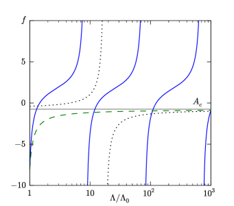
Figure 1: Examples of dependence of the counterterm coupling constant $f$ for two lowest angular momentum quantum numbers $l$ and the coupling constant $g$ in Eq. (1) equal $9/(8m)$, which is a critical value for $l=1$, with the corresponding value of $A_{c}=-0.75$ indicated by a horizontal line. For $l=0$, $f$ exhibits limit-cycle (solid line). For $l=1$, $f$ approaches $A_{c}$ in a logarithmic fashion that characterizes approach to zero in asymptotic-freedom (dashed line). In both cases $f(\Lambda_{0})=-8.0$. Setting $f(\Lambda_{0})=-0.4$, which is above $A_{c}$, one obtains an example of the Landau pole (dotted line).

When $\alpha=\alpha_{lc}$, in which case $l=0$ corresponds to the well-known critical value $\alpha_{0c}=1/4$, one obtains

$$f-A_{c}={f_{0}-A_{c}\over 1-(f_{0}-A_{c})\ln{\Lambda\over\Lambda_{0}}}\ ,$$ (16)

where, for the critical value of $l$ for this $\alpha$, $A_{c}=f_{+}=f_{-}=-L/2$. Thus, considering only $\Lambda$ that increases above some $\Lambda_{0}$, one obtains the renormalized Hamiltonians with $f$ that approaches the fixed point $f=A_{c}$ in a logarithmic way characteristic of the asymptotic-freedom when one starts from $f_{0}<A_{c}$, or deviates from $A_{c}$ in the fashion of triviality, associated with the Landau pole, when $f_{0}>A_{c}$. This result extends the previously noted relationship between renormalization group limit-cycle and asymptotic-freedom behaviors [37] to the case of $-g/r^{2}$ potential in the Schrödinger equation, since $\alpha\to\alpha_{lc}$ from above implies $B\to 0$ and the cycle period growing to infinity. On the other hand, when $\alpha$ approaches $\alpha_{lc}$ from below, the distance between the two fixed points $f_{-}$ and $f_{+}$ for the critical value of $l$ shrinks to zero.

Examples of behavior of the constant $f$ as a function of the cutoff $\Lambda$ are shown in Figs. 1 and 2. The figures display the flow of the couplings for three different angular momenta, $l=0,1,2$. The coupling constant $\alpha$ is set to the critical value for $l=1$. It is visible that one and the same Hamiltonian exhibits various renormalization group behaviors in different partial waves. Figure 3 presents the beta-functions for the same cases. The asymptotic freedom case appears in the vicinity of one fixed point that can be thought to result from a collision of two fixed-points, in analogy to the $s$-wave analysis in Ref. [16]. Figure 3 also shows that the asymptotic-freedom case can be seen as resulting from the limit cycle when the minimum of beta-function reaches zero and the period of the cycle grows to infinity. In each case one can adjust the corresponding value of $f_{0}$ to a desired binding energy or a phase shift at a selected energy. However, a complete description of various types of bound-state and scattering observables for different choices of finite parameters in the renormalized Hamiltonians is beyond the scope of this paper.

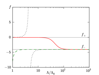
Figure 2: Examples of dependence of the counterterm coupling constant $f$ for $l=2$ and the same coupling constant $g=9/(8m)$ as in Fig. 1, critical for $l=1$. The two fixed points are $f_{+}=-0.05$ and $f_{-}=-4.05$. For $f(\Lambda_{0})=f_{+}-10^{-6}$, $f$ flows toward $f_{-}$ (solid line). For $f(\Lambda_{0})=f_{+}+10^{-2}$, $f$ develops the Landau pole (dotted line). For $f(\Lambda_{0})=-8.0<f_{-}$, $f$ increases to $f_{-}$ (dashed line).

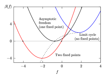
Figure 3: Beta-functions of the coupling constants $f$ in partial waves $l=0,1,2$, corresponding to the renormalization group behaviors illustrated in Figs. 1 and 2. The dotted line is the curve on which lie the minima of all beta-functions, parameterized by $l$, see Eq. (13). As $l$ increases, and $\alpha$ is fixed, the minimum goes down the line. When $\alpha$ is increased, the whole line shifts up and right (and deforms) allowing more partial waves to enter into the limit cycle regime. This illustrates how transition from fixed points through asymptotic freedom to limit cycle occurs.

4 Conclusion

Simplicity of the renormalization procedure for $-g/r^{2}$ potential in the Schrödinger equation, carried out here using the RGT of Wilsonian type, results from neglecting the ratio of eigenvalues $E$ to the floating cutoff $\Lambda$. Inclusion of this ratio in the RGT can be carried out according to the steps described in Ref. [38]. For example, one can employ an expansion in powers of $E/\Lambda$ and establish corrections needed in $H_{\Delta}$ to accelerate convergence of the family $H_{\Lambda}$ on the limit cycle when $\Lambda$ is lowered. When in practice the ratio $E/\Lambda$ is not sufficiently small and the expansion in its powers is not efficient, one can switch to the similarity renormalization group procedure [39, 40]. In principle, the similarity procedure avoids dependence on the eigenvalues and can be employed as in Refs. [37, 41].
 
Acknowledgements

Authors thank the Faculty of Physics at the University of Warsaw for support of the course Introduction to Renormalization within which the research reported here was carried out.

References

- [1] K. M. Case, Phys. Rev. 80 (1950) 797. doi:10.1103/PhysRev.80.797.
- [2] S. R. Beane, P. F. Bedaque, L. Childress, A. Kryjevski, J. McGuire, U. van Kolck, Phys. Rev. A 64 (2001) 042103. doi:10.1103/PhysRevA.64.042103.
- [3] M. Bawin, S. A. Coon, Phys. Rev. A 67 (2003) 042712. doi:10.1103/PhysRevA.67.042712.
- [4] S. A. Coon, B. Holstein, Am. J. Phys. 70 (2002) 513. doi:10.1119/1.1456071.
- [5] E. Braaten, D. Phillips, Phys. Rev. A 70 (2004) 052111. doi:10.1103/PhysRevA.70.052111.
- [6] H.-W. Hammer, B. G. Swingle, Ann. Phys. 321 (2006) 306. doi:10.1016/j.aop.2005.04.017.
- [7] H.-W. Hammer, R. Higa, Eur. Phys. J. A 37 (2008) 193. doi:10.1140/epja/i2008-10617-3.
- [8] B. Long, U. van Kolck, Ann. Phys. 323 (2008) 1304. doi:10.1016/j.aop.2008.01.003.
- [9] M. P. Valderrama, E. R. Arriola, Ann. Phys. 323 (2008) 1037. doi:10.1016/j.aop.2007.08.003.
- [10] D. B. Kaplan, J.-W. Lee, D. T. Son, M. A. Stephanov, Phys. Rev. D 80 (2009) 125005. doi:10.1103/PhysRevD.80.125005.
- [11] T. Y. Cao, S. S. Schweber, The conceptual foundations and the philosophical aspects of renormalization theory, Synthese 97 (1) (1993) 33–108. doi:10.1007/BF01255832.
-
[12]
T. Y. Cao (Ed.), Conceptual foundations of
quantum field theory. Proceedings, Symposium and Workshop, Boston, USA, March
1-3, 1996, CUP, CUP, Cambridge, UK, 1999.
URL http://www.cambridge.org/ch/academic/subjects/physics/history-philosophy-and-foundations-physics/conceptual-foundations-quantum-field-theory - [13] K. G. Wilson, Phys. Rev. B 140 (1965) 445. doi:10.1103/PhysRev.140.B445.
- [14] K. G. Wilson, Phys. Rev. D 2 (1970) 1438. doi:10.1103/PhysRevD.2.1438.
- [15] K. G. Wilson, Phys. Rev. D3 (1971) 1818. doi:10.1103/PhysRevD.3.1818.
- [16] S. Moroz, R. Schmidt, Annals Phys. 325 (2010) 491–513. doi:10.1016/j.aop.2009.10.002.
- [17] S. D. Głazek, K. G. Wilson, Phys. Rev. Lett. 89 (2002) 230401. doi:10.1103/PhysRevLett.89.230401.
- [18] S. D. Głazek, K. G. Wilson, Erratum, Phys. Rev. Lett. 92 (2004) 139901. doi:10.1103/PhysRevLett.92.139901.
- [19] L. H. Thomas, Phys. Rev. 47 (1935) 903. doi:10.1103/PhysRev.47.903.
- [20] V. Efimov, Phys. Lett. B 33 (1970) 563. doi:10.1016/0370-2693(70)90349-7.
- [21] V. Efimov, Nucl. Phys. A 210 (1973) 157. doi:10.1016/0375-9474(73)90510-1.
- [22] P. F. Bedaque, H.-W. Hammer, U. van Kolck, Phys. Rev. Lett. 82 (1999) 463. doi:10.1103/PhysRevLett.82.463.
- [23] R. F. Mohr, R. J. Furnstahl, H.-W. Hammer, R. J. Perry, K. G. Wilson, Ann. Phys. 321 (2006) 225. doi:10.1016/j.aop.2005.10.002.
- [24] H. E. Camblong, L. N. Epele, H. Fanchiotti, C. A. G. Canal, Phys. Rev. Lett. 85 (2000) 1590. doi:10.1103/PhysRevLett.85.1590.
- [25] H. E. Camblong, L. N. Epele, H. Fanchiotti, C. A. G. Canal, Phys. Rev. Lett. 87 (2001) 220402. doi:10.1103/PhysRevLett.87.220402.
- [26] H. E. Camblong, C. R. Ordóñez, Phys. Rev. D 68 (2003) 125013. doi:10.1103/PhysRevD.68.125013.
- [27] J. Kosterlitz, J. Phys. C 7 (1974) 1046. doi:10.1088/0022-3719/7/6/005.
- [28] E. B. Kolomeisky, J. P. Straley, Phys. Rev. B 46 (1992) 13942. doi:10.1103/PhysRevB.46.13942.
- [29] J. M. Maldacena, Adv. Theor. Math. Phys. 2 (1998) 231. doi:10.1023/A:1026654312961.
- [30] V. de Alfaro, S. Fubini, G. Furlan, Nuovo Cim. A 34 (1976) 569. doi:10.1007/BF02785666.
- [31] S. J. Brodsky, G. F. de Teramond, H. G. Dosch, J. Erlich, Phys. Rept. 584 (2015) 1. doi:10.1016/j.physrep.2015.05.001.
- [32] D. Dietrich, F. Sannino, Phys. Rev. D 75 (2007) 085018. doi:10.1103/PhysRevD.75.085018.
- [33] T. Banks, A. Zaks, Nucl. Phys. B 196 (1982) 189. doi:10.1016/0550-3213(82)90035-9.
- [34] T. Appelquist, et al., Phys. Rev. D 93 (2016) 114514. doi:10.1103/PhysRevD.93.114514.
- [35] S. R. Coleman, E. J. Weinberg, Phys. Rev. D 7 (1973) 1888. doi:10.1103/PhysRevD.7.1888.
- [36] K. G. Wilson, T. S. Walhout, A. Harindranath, W.-M. Zhang, R. J. Perry, S. D. Głazek, Phys. Rev. D 49 (1994) 6720; Sec. VII B. doi:10.1103/PhysRevD.49.6720.
- [37] S. D. Głazek, Phys. Rev. D 75 (2007) 025005. doi:10.1103/PhysRevD.75.025005.
- [38] S. D. Głazek, K. G. Wilson, Phys. Rev. B 69 (2004) 094304. doi:10.1103/PhysRevB.69.094304.
- [39] S. D. Głazek, K. G. Wilson, Phys. Rev. D 48 (1993) 5863. doi:10.1103/PhysRevD.48.5863.
- [40] S. D. Głazek, K. G. Wilson, Phys. Rev. D 49 (1994) 4214. doi:10.1103/PhysRevD.49.4214.
- [41] P. Niemann, H.-W. Hammer, Few-Body Syst. 56 (2015) 869. doi:10.1007/s00601-015-1001-0.