Abstract

The article concerns compressed sensing methods in the quaternion algebra. We prove that it is possible to uniquely reconstruct – by $\ell_{1}$-norm minimization – a sparse quaternion signal from a limited number of its linear measurements, provided the quaternion measurement matrix satisfies so-called restricted isometry property with a sufficiently small constant. We also provide error estimates for the reconstruction of a non-sparse quaternion signal in the noisy and noiseless cases.

1 Introduction

E. Candés et al. showed that – in the real or complex setting – if a measurement matrix satisfies so-called restricted isometry property (RIP) with a sufficiently small constant, then every sparse signal can be uniquely reconstructed from a limited number of its linear measurements as a solution of a convex program of $\ell_{1}$-norm minimization (see e.g. [7, 8, 9] and [14] for more references). Sparsity of the signal is a natural assumption – most of well known signals have a sparse representation in an appropriate basis (e.g. wavelet representation of an image). Moreover, if the original signal was not sparse, the same minimization procedure provides a good sparse approximation of the signal and the procedure is stable in the sense that the error is bounded above by the $\ell_{1}$-norm of the difference between the original signal and its best sparse approximation.

For a certain time the attention of the researchers in the theory of compressed sensing has mostly been focused on real and complex signals. Over the last decade there have been published results of numerical experiments suggesting that the compressed sensing methods can be successfully applied also in the quaternion algebra [4, 17, 27], however, until recently there were no theoretical results that could explain the success of these experiments. The aim of our research is to develop theoretical background of the compressed sensing theory in the quaternion algebra.

Our first step towards this goal was proving that one can uniquely reconstruct a sparse quaternion signal – by $\ell_{1}$-norm minimization – provided the real measurement matrix satisfies the RIP (for quaternion vectors) with a sufficiently small constant ([1, Corrolary 5.1]). This result can be directly applied since any real matrix satisfying the RIP for real vectors, satisfies the RIP for quaternion vectors with the same constant ([1, Lemma 3.2]). We also want to point out a very interesting recent result of N. Gomes, S. Hartmann and U. Kähler concerning the quaternion Fourier matrices – arising in colour representation of images. They showed that with high probability such matrices allow a sparse reconstruction by means of the $\ell_{1}$-minimization [15, Theorem 3.2]. Their proof, however, is straightforward and does not use the notion of RIP.

The generalization of compressed sensing to the quaternion algebra would be significant due to their wide applications. Apart from the classical applications (in quantum mechanics and for the description of 3D solid body rotations), quaternions have also been used in 3D and 4D signal processing [22], in particular to represent colour images (e.g. in the RGB or CMYK models). Due to the extension of classical tools (like the Fourier transform [13]) to the quaternion algebra it is possible to investigate colour images without need of treating each component separately [11, 13]. That is why quaternions have found numerous applications in image filtering, image enhancement, pattern recognition, edge detection and watermarking [12, 16, 18, 19, 21, 24, 26]. There has also been proposed a dual-tree quaternion wavelet transform in a multiscale analysis of geometric image features [10]. For this purpose an alternative representation of quaternions is used – through its magnitude (norm) and three phase angles: two of them encode phase shifts while the third contains image texture information [5]. In view of numerous articles presenting results of numerical experiments of quaternion signal processing and their possible applications, there is a natural need of further thorough theoretical investigations in this field.

In this article we extend the fundamental result of the compressed sensing theory to the quaternion case, namely we show that if a quaternion measurement matrix satisfies the RIP with a sufficiently small constant, then it is possible to reconstruct sparse quaternion signals from a small number of their measurements via $\ell_{1}$-norm minimization (Corollary 5.1). We also estimate the error of reconstruction of a non-sparse signal from exact and noisy data (Theorem 4.1). Note that these results not only generalize the previous ones [1, Theorem 4.1, Corrolary 5.1] but also improve them by decreasing the error estimation’s constants. This enhancement was possible due to using algebraic properties of quaternion Hermitian matrices (Lemma 2.1) to derive characterization of the restricted isometry constants (Lemma 3.2) analogous to the real and complex case. Consequently, one can carefully follow steps of the classical Candés’ proof [7] with caution to the non-commutativity of quaternion multiplication.

It is known that e.g. real Gaussian and Bernoulli random matrices, also partial Discrete Fourier Transform matrices satisfy the RIP (with overwhelming probability) [14], however, until recently there were no known examples of quaternion matrices satisfying this condition. It has been believed that quaternion Gaussian random matrices satisfy RIP and, therefore, they have been widely used in numerical experiments [4, 17, 27] but there was a lack of theoretical justification of this conviction. In the subsequent article [2] we prove that this hypothesis is true, i.e. quaternion Gaussian matrices satisfy the RIP, and we provide estimates on matrix sizes that guarantee the RIP with overwhelming probability. This result, together with the main results of this article (Theorem 4.1, Corollary 5.1), constitute the theoretical foundation of the classical compressed sensing methods in the quaternion algebra.

The article is organized as follows. First, we recall basic notation and facts concerning the quaternion algebra with particular emphasis put on the properties of Hermitian form and Hermitian matrices. The third section is devoted to the RIP and characterization of the restricted isometry constants in terms of Hermitian matrix norm. The fourth and fifth sections contain proofs of the main results of the article. In the sixth section we present results of numerical experiments illustrating our results – we may see, in particular, that the rate of perfect reconstructions in the quaternion case is higher than in the real case experiment with the same parameters. We conclude with a short résumé of the obtained results and our further research perspectives.

2 Algebra of quaternions

Denote by $\mathbb{H}$ the algebra of quaternions

$$q=a+b\mathbf{i}+c\mathbf{j}+d\mathbf{k},\quad\textrm{where}\quad a,b,c,d\in\mathbb{R},$$

endowed with the standard norm

$$|q|=\sqrt{q\overline{q}}=\sqrt{a^{2}+b^{2}+c^{2}+d^{2}},$$

where $\overline{q}=a-b\mathbf{i}-c\mathbf{j}-d\mathbf{k}$ is the conjugate of $q$.

Recall that multiplication is associative but in general not commutative in the quaternion algebra and is defined by the following rules

$$\mathbf{i}^{2}=\mathbf{j}^{2}=\mathbf{k}^{2}=\mathbf{i}\mathbf{j}\mathbf{k}=-1$$

and

$$\mathbf{i}\mathbf{j}=-\mathbf{j}\mathbf{i}=\mathbf{k},\quad\mathbf{j}\mathbf{k}=-\mathbf{k}\mathbf{j}=\mathbf{i},\quad\mathbf{k}\mathbf{i}=-\mathbf{i}\mathbf{k}=\mathbf{j}.$$

Multiplication is distributive with respect to addition and has a neutral element $1\in\mathbb{H}$, hence $\mathbb{H}$ forms a ring, which is usually called a noncommutative field. We also have the property that

$$\overline{q\cdot w}=\overline{w}\cdot\overline{q}\quad\textrm{for any}\quad q,w\in\mathbb{H}.$$

In what follows we will interpret signals as vectors with quaternion coordinates, i.e. elements of $\mathbb{H}^{n}$. Algebraically $\mathbb{H}^{n}$ is a module over the ring $\mathbb{H}$, usually called the quaternion vector space. We will also consider matrices with quaternion entries with usual multiplication rules.

For any matrix $\mathbf{\Phi}\in\mathbb{H}^{m\times n}$ with quaternion entries by $\mathbf{\Phi}^{*}$ we denote the adjoint matrix, i.e. $\mathbf{\Phi}^{*}=\overline{\mathbf{\Phi}}^{T}$, where $T$ is the transpose. The same notation applies to quaternion vectors $\mathbbm{x}\in\mathbb{H}^{n}$ which can be interpreted as one-column matrices $\mathbbm{x}\in\mathbb{H}^{n\times 1}$. Obviously $\left(\mathbf{\Phi}^{*}\right)^{*}=\mathbf{\Phi}$.

A matrix $\mathbf{\Phi}\in\mathbb{H}^{m\times n}$ defines a $\mathbb{H}$-linear transformation $\mathbf{\Phi}:\mathbb{H}^{n}\to\mathbb{H}^{m}$ (in terms of the right quaternion vector space, i.e. considering the right scalar multiplication) which acts by the standard matrix-vector multiplication:

$$\mathbf{\Phi}(\mathbbm{x}+\mathbbm{y})=\mathbf{\Phi}\mathbbm{x}+\mathbf{\Phi}\mathbbm{y}\quad\textrm{and}\quad\mathbf{\Phi}(\mathbbm{x}q)=(\mathbf{\Phi}\mathbbm{x})q\quad\textrm{for any}\quad\mathbbm{x},\mathbbm{y}\in\mathbb{H}^{n},\;q\in\mathbb{H}.$$

We also have that

$$(\mathbf{\Phi}q)^{*}=\overline{q}\mathbf{\Phi}^{*},\quad(q\mathbf{\Phi})^{*}=\mathbf{\Phi}^{*}\overline{q},\quad(\mathbf{\Phi}\mathbbm{x})^{*}=\mathbbm{x}^{*}\mathbf{\Phi}^{*},\quad(\mathbf{\Phi}\mathbf{\Psi})^{*}=\mathbf{\Psi}^{*}\mathbf{\Phi}^{*}$$

for all $\mathbf{\Phi}\in\mathbb{H}^{m\times n}$, $q\in\mathbb{H}$, $\mathbbm{x}\in\mathbb{H}^{n}$, $\mathbf{\Psi}\in\mathbb{H}^{n\times p}$.

For any $n\in\mathbb{N}$ we introduce the following Hermitian form $\left\langle{\cdot,\cdot}\right\rangle\colon\mathbb{H}^{n}\times\mathbb{H}^{n}\to\mathbb{H}$ with quaternion values:

$$\left\langle{\mathbbm{x},\mathbbm{y}}\right\rangle=\mathbbm{y}^{*}\mathbbm{x}=\sum_{i=1}^{n}\overline{y_{i}}x_{i},\quad\textrm{where}\quad\mathbbm{x}=(x_{1},\ldots,x_{n})^{T},\;\mathbbm{y}=(y_{1},\ldots,y_{n})^{T}\in\mathbb{H}^{n}$$

and $T$ is the transpose. Denote also

$$\left\lVert{\mathbbm{x}}\right\rVert_{2}=\sqrt{\left\langle{\mathbbm{x},\mathbbm{x}}\right\rangle}=\sqrt{\sum_{i=1}^{n}|x_{i}|^{2}},\quad\textrm{for any }\mathbbm{x}=(x_{1},\ldots,x_{n})^{T}\in\mathbb{H}^{n}.$$

It is straightforward calculation to verify that $\left\langle{\cdot,\cdot}\right\rangle$ satisfies the following properties of an inner product for all $\mathbbm{x},\mathbbm{y},\mathbbm{z}\in\mathbb{H}^{n}$ and $q\in\mathbb{H}$.

• $\displaystyle\overline{\left\langle{\mathbbm{x},\mathbbm{y}}\right\rangle}=\left\langle{\mathbbm{y},\mathbbm{x}}\right\rangle$.

• $\displaystyle\left\langle{\mathbbm{x}q,\mathbbm{y}}\right\rangle=\left\langle{\mathbbm{x},\mathbbm{y}}\right\rangle q$.

• $\displaystyle\left\langle{\mathbbm{x}+\mathbbm{y},\mathbbm{z}}\right\rangle=\left\langle{\mathbbm{x},\mathbbm{z}}\right\rangle+\left\langle{\mathbbm{y},\mathbbm{z}}\right\rangle$.

• $\displaystyle\left\langle{\mathbbm{x},\mathbbm{x}}\right\rangle=\left\lVert{\mathbbm{x}}\right\rVert_{2}^{2}\geq 0$ and $\displaystyle\left\lVert{\mathbbm{x}}\right\rVert_{2}^{2}=0\quad\iff\quad\mathbbm{x}=\mathbf{0}$.

Hence $\left\lVert{\cdot}\right\rVert_{2}$ satisfies the axioms of a norm in $\mathbb{H}^{n}$.

By carefully following the classical steps of the proof we also get the Cauchy-Schwarz inequality (cf.[1, Lemma 2.2]).

$$|\left\langle{\mathbbm{x},\mathbbm{y}}\right\rangle|\leq\left\lVert{\mathbbm{x}}\right\rVert_{2}\cdot\left\lVert{\mathbbm{y}}\right\rVert_{2}$$

for any $\mathbbm{x},\mathbbm{y}\in\mathbb{H}^{n}$.

Notice that for $\mathbf{\Phi}\in\mathbb{H}^{m\times n}$ the matrix $\mathbf{\Phi}^{*}$ defines the adjoint $\mathbb{H}$-linear transformation since

$$\left\langle{\mathbbm{x},\mathbf{\Phi}^{*}\mathbbm{y}}\right\rangle=\left(\mathbf{\Phi}^{*}\mathbbm{y}\right)^{*}\mathbbm{x}=\mathbbm{y}^{*}\mathbf{\Phi}\mathbbm{x}=\left\langle{\mathbf{\Phi}\mathbbm{x},\mathbbm{y}}\right\rangle\quad\textrm{for}\quad\mathbbm{x}\in\mathbb{H}^{n},\mathbbm{y}\in\mathbb{H}^{m}.$$

Recall also that a linear transformation (matrix) $\mathbf{\Psi}\in\mathbb{H}^{n\times n}$ is called Hermitian if $\mathbf{\Psi}^{*}=\mathbf{\Psi}$. Obviously $\mathbf{\Phi}^{*}\mathbf{\Phi}$ is Hermitian for any $\mathbf{\Phi}\in\mathbb{H}^{m\times n}$.

In the next section we will use the following property of Hermitian matrices.

Lemma 2.1.

Suppose $\mathbf{\Psi}\in\mathbb{H}^{n\times n}$ is Hermitian. Then

$$\left\lVert{\mathbf{\Psi}}\right\rVert_{2\to 2}=\max_{\mathbbm{x}\in\mathbb{H}^{n},\left\lVert{\mathbbm{x}}\right\rVert_{2}=1}\left|\left\langle{\mathbf{\Psi}\mathbbm{x},\mathbbm{x}}\right\rangle\right|=\max_{\mathbbm{x}\in\mathbb{H}^{n}\setminus\{\mathbf{0}\}}\frac{\left|\left\langle{\mathbf{\Psi}\mathbbm{x},\mathbbm{x}}\right\rangle\right|}{\left\lVert{\mathbbm{x}}\right\rVert_{2}^{2}},$$

where $\left\lVert{\cdot}\right\rVert_{2\to 2}$ is the standard operator norm in the right quaternion vector space $\mathbb{H}^{n}$ endowed with the norm $\left\lVert{\cdot}\right\rVert_{2}$, i.e.

$$\left\lVert{\mathbf{\Psi}}\right\rVert_{2\to 2}=\max_{\mathbbm{x}\in\mathbb{H}^{n}\setminus\{\mathbf{0}\}}\frac{\left\lVert{\mathbf{\Psi}\mathbbm{x}}\right\rVert_{2}}{\left\lVert{\mathbbm{x}}\right\rVert_{2}}=\max_{\mathbbm{x}\in\mathbb{H}^{n},\left\lVert{\mathbbm{x}}\right\rVert_{2}=1}\left\lVert{\mathbf{\Psi}\mathbbm{x}}\right\rVert_{2}.$$

Proof.

Recall that a Hermitian matrix has real (right) eigenvalues [20]. Moreover, there exists an orthonormal (in terms of the $\mathbb{H}$-linear form $\left\langle{\cdot,\cdot}\right\rangle$) base of $\mathbb{H}^{n}$ consisting of eigenvectors $\mathbbm{x}_{i}$ corresponding to eigenvalues $\lambda_{i}\in\mathbb{R}$, $i=1,\ldots,n$ (cf.[20, Theorem 5.3.6. (c)]), i.e.

$$\mathbf{\Psi}\mathbbm{x}_{i}=\mathbbm{x}_{i}\lambda_{i}\quad\textrm{and}\quad\left\langle{\mathbbm{x}_{i},\mathbbm{x}_{j}}\right\rangle=\mathbbm{x}_{j}^{*}\mathbbm{x}_{i}=\delta_{i,j}\quad\textrm{for}\quad i,j=1,\ldots,n.$$

Denote $\lambda_{\max}=\max_{i}|\lambda_{i}|$. Then $\left\lVert{\mathbf{\Psi}}\right\rVert_{2\to 2}=\lambda_{\max}$. Indeed, for any $\mathbbm{x}=\sum\limits_{i=1}^{n}\mathbbm{x}_{i}\alpha_{i}\in\mathbb{H}^{n}$ with $\left\lVert{\mathbbm{x}}\right\rVert_{2}^{2}=\sum\limits_{i=1}^{n}|\alpha_{i}|^{2}=1$, since $\mathbbm{x}_{i}$ are orthonormal, we have

$$\left\lVert{\mathbf{\Psi}\mathbbm{x}}\right\rVert_{2}^{2}=\left\lVert{\sum_{i=1}^{n}\mathbf{\Psi}\mathbbm{x}_{i}\alpha_{i}}\right\rVert_{2}^{2}=\left\lVert{\sum_{i=1}^{n}\mathbbm{x}_{i}\lambda_{i}\alpha_{i}}\right\rVert_{2}^{2}=\sum_{i=1}^{n}\left|\lambda_{i}\alpha_{i}\right|^{2}\leq\lambda_{\max}\underbrace{\sum_{i=1}^{n}\left|\alpha_{i}\right|^{2}}_{=1}$$

and for the appropriate eigenvector $\mathbbm{x}_{i}$ for which $|\lambda_{i}|=\lambda_{\max}$,

$$\left\lVert{\mathbf{\Psi}\mathbbm{x}_{i}}\right\rVert_{2}=\left\lVert{\mathbbm{x}_{i}\lambda_{i}}\right\rVert_{2}=\lambda_{\max}\left\lVert{\mathbbm{x}_{i}}\right\rVert_{2}=\lambda_{\max}.$$

On the other hand, since $\lambda_{i}$ are real,

$$\left\langle{\mathbf{\Psi}\mathbbm{x},\mathbbm{x}}\right\rangle =\mathbbm{x}^{*}\mathbf{\Psi}\mathbbm{x}=\left(\sum_{i=1}^{n}\mathbbm{x}_{i}\alpha_{i}\right)^{*}\left(\sum_{j=1}^{n}\mathbf{\Psi}\mathbbm{x}_{j}\alpha_{j}\right)=\left(\sum_{i=1}^{n}\overline{\alpha_{i}}\mathbbm{x}_{i}^{*}\right)\left(\sum_{j=1}^{n}\mathbbm{x}_{j}\lambda_{j}\alpha_{j}\right)$$

$$=\sum_{i=1}^{n}\overline{\alpha_{i}}\lambda_{i}\alpha_{i}\stackrel{{\scriptstyle\lambda_{i}\in\mathbb{R}}}{{=}}\sum_{i=1}^{n}\lambda_{i}|\alpha_{i}|^{2}.$$

Hence

$$\left|\left\langle{\mathbf{\Psi}\mathbbm{x},\mathbbm{x}}\right\rangle\right|\leq\lambda_{\max}\sum\limits_{i=1}^{n}|\alpha_{i}|^{2}=\lambda_{\max}$$

and – again – for the appropriate eigenvector the last two quantities are equal. The result follows. ∎

In what follows we will consider $\left\lVert{\cdot}\right\rVert_{p}$ norms for quaternion vectors $\mathbbm{x}\in\mathbb{H}^{n}$ defined in the standard way:

$$\left\lVert{\mathbbm{x}}\right\rVert_{p}=\left(\sum_{i=1}^{n}|x_{i}|^{p}\right)^{1/p},\quad\textrm{for}\quad p\in[1,\infty)$$

and

$$\left\lVert{\mathbbm{x}}\right\rVert_{\infty}=\max_{1\leq i\leq n}|x_{i}|,$$

where $\mathbbm{x}=(x_{1},\ldots,x_{n})^{T}$. We will also apply the usual notation for the cardinality of the support of $\mathbbm{x}$, i.e.

$$\left\lVert{\mathbbm{x}}\right\rVert_{0}=\#\mathrm{supp}(\mathbbm{x}),\quad\textrm{where}\quad\mathrm{supp}(\mathbbm{x})=\{i\in\{1,\ldots,n\}\colon x_{i}\neq 0\}.$$

3 Restricted Isometry Property

Recall that we call a vector (signal) $\mathbbm{x}\in\mathbb{H}^{n}$ $s$-sparse if it has at most $s$ nonzero coordinates, i.e.

$$\left\lVert{\mathbbm{x}}\right\rVert_{0}\leq s.$$

As it was mentioned in the introduction, one of the conditions which guarantees exact reconstruction of a sparse real signal from a few number of its linear measurements is that the measurement matrix satisfies so-called restricted isometry property (RIP) with a sufficiently small constant. The notion of restricted isometry constants was introduced by Candès and Tao in [9]. Here we generalize it to quaternion signals.

Definition 3.1.

Let $s\in\mathbb{N}$ and $\mathbf{\Phi}\in\mathbb{H}^{m\times n}$. We say that $\mathbf{\Phi}$ satisfies the $s$-restricted isometry property (for quaternion vectors) with a constant $\delta_{s}\geq 0$ if

$$\left(1-\delta_{s}\right)\left\lVert{\mathbbm{x}}\right\rVert_{2}^{2}\leq\left\lVert{\mathbf{\Phi}\mathbbm{x}}\right\rVert_{2}^{2}\leq\left(1+\delta_{s}\right)\left\lVert{\mathbbm{x}}\right\rVert_{2}^{2}$$ (3.1)

for all $s$-sparse quaternion vectors $\mathbbm{x}\in\mathbb{H}^{n}$. The smallest number $\delta_{s}\geq 0$ with this property is called the $s$-restricted isometry constant.

Note that we can define $s$-restricted isometry constants for any matrix $\mathbf{\Phi}\in\mathbb{H}^{m\times n}$ and any number $s\in\{1,\ldots,n\}$. It has been proved that if a real matrix $\mathbf{\Phi}\in\mathbb{R}^{m\times n}$ satisfies the inequality (3.1) for real $s$-sparse vectors $\mathbbm{x}\in\mathbb{R}^{n}$, then it also satisfies it – with the same constant $\delta_{s}$ – for $s$-sparse quaternion vectors $\mathbbm{x}\in\mathbb{H}^{n}$ [1, Lemma 3.2].

The following lemma extends an analogous result, known for real and complex matrices [14], to the quaternion case. As is it accustomed, for a matrix $\mathbf{\Phi}\in\mathbb{H}^{m\times n}$ and a set of indices $S\subset\{1,\ldots,n\}$ with $\#S=s$ by $\mathbf{\Phi}_{S}\in\mathbb{H}^{m\times s}$ we denote the matrix consisting of columns of $\mathbf{\Phi}$ with indices in the set $S$.

Lemma 3.2.

The $s$-restricted isometry constant $\delta_{s}$ of a matrix $\mathbf{\Phi}\in\mathbb{H}^{m\times n}$ equivalently equals

$$\delta_{s}=\max_{S\subset\{1,\ldots,n\},\#S\leq s}\left\lVert{\mathbf{\Phi}_{S}^{*}\mathbf{\Phi}_{S}-\mathbf{Id}}\right\rVert_{2\to 2}.$$

Proof.

We proceed as in [14, Chapter 6]. Fix any $s\in\{1,\ldots,n\}$ and $S\subset\{1,\ldots,n\}$ with $\#S\leq s$. Notice that the condition (3.1) can be equivalently rewritten as

$$\left|\left\lVert{\mathbf{\Phi}_{S}\mathbbm{x}}\right\rVert_{2}^{2}-\left\lVert{\mathbbm{x}}\right\rVert_{2}^{2}\right|\leq\delta_{s}\left\lVert{\mathbbm{x}}\right\rVert_{2}^{2}\quad\textrm{for all}\quad\mathbbm{x}\in\mathbb{H}^{s},$$

where $\delta_{s}$ is the $s$-restricted isometry constant of $\mathbf{\Phi}$. The left hand side equals

$$\left|\left\lVert{\mathbf{\Phi}_{S}\mathbbm{x}}\right\rVert_{2}^{2}-\left\lVert{\mathbbm{x}}\right\rVert_{2}^{2}\right|\leq\delta_{s}\left\lVert{\mathbbm{x}}\right\rVert_{2}^{2}=\left|\left\langle{\mathbf{\Phi}_{S}\mathbbm{x},\mathbf{\Phi}_{S}\mathbbm{x}}\right\rangle-\left\langle{\mathbbm{x},\mathbbm{x}}\right\rangle\right|=\left|\left\langle{\left(\mathbf{\Phi}_{S}^{*}\mathbf{\Phi}_{S}-\mathbf{Id}\right)\mathbbm{x},\mathbbm{x}}\right\rangle\right|$$

and by the Lemma 2.1, since the matrix $\mathbf{\Phi}_{S}^{*}\mathbf{\Phi}_{S}-\mathbf{Id}$ is Hermitian, we get that

$$\max_{\mathbbm{x}\in\mathbb{H}^{s}\setminus\{\mathbf{0}\}}\frac{\left|\left\langle{\left(\mathbf{\Phi}_{S}^{*}\mathbf{\Phi}_{S}-\mathbf{Id}\right)\mathbbm{x},\mathbbm{x}}\right\rangle\right|}{\left\lVert{\mathbbm{x}}\right\rVert_{2}^{2}}=\left\lVert{\mathbf{\Phi}_{S}^{*}\mathbf{\Phi}_{S}-\mathbf{Id}}\right\rVert_{2\to 2}.$$

Arbitrary choice of $s$ and $S$ finishes the proof. ∎

The next result is an important tool in the proof of Theorem 4.1. Having the above equivalence and the Cauchy-Schwarz inequality we are able to obtain for quaternion vectors the same estimate as in the real and complex case (cf. [7, Lemma 2.1] and [14, Proposition 6.3]).

Lemma 3.3.

Let $\delta_{s}$ be the $s$-restricted isometry constant for a matrix $\mathbf{\Phi}\in\mathbb{H}^{m\times n}$ for $s\in\{1,\ldots,n\}$. For any pair of $\mathbbm{x},\mathbbm{y}\in\mathbb{H}^{n}$ with disjoint supports and such that $\left\lVert{\mathbbm{x}}\right\rVert_{0}\leq s_{1}$ and $\left\lVert{\mathbbm{y}}\right\rVert_{0}\leq s_{2}$, where $s_{1}+s_{2}\leq n$, we have that

$$\left|\left\langle{\mathbf{\Phi}\mathbbm{x},\mathbf{\Phi}\mathbbm{y}}\right\rangle\right|\leq\delta_{s_{1}+s_{2}}\left\lVert{\mathbbm{x}}\right\rVert_{2}\left\lVert{\mathbbm{y}}\right\rVert_{2}.$$

Proof.

In this proof we will use the following notation: for any vector $\mathbbm{x}\in\mathbb{H}^{n}$ and a set of indices $S\subset\{1,\ldots,n\}$ with $\#S=s$ by $\mathbbm{x}_{|S}\in\mathbb{H}^{s}$ we denote the vector of $\mathbbm{x}$-coordinates with indices in $S$.

Take any vectors $\mathbbm{x},\mathbbm{y}\in\mathbb{H}^{n}$ satisfying the assumptions of the lemma and denote $S=\mathrm{supp}(\mathbbm{x})\cup\mathrm{supp}(\mathbbm{y})$. Obviously $\#S=s_{1}+s_{2}$. Since $\mathbbm{x}$ and $\mathbbm{y}$ have disjoint supports, they are orthogonal, i.e. $\left\langle{\mathbbm{x},\mathbbm{y}}\right\rangle=\left\langle{\mathbbm{x}_{|S},\mathbbm{y}_{|S}}\right\rangle=0$. Using the Cauchy-Schwarz inequality and Lemma 3.2 we get that

$$\left|\left\langle{\mathbf{\Phi}\mathbbm{x},\mathbf{\Phi}\mathbbm{y}}\right\rangle\right| =\left|\left\langle{\mathbf{\Phi}_{S}\mathbbm{x}_{|S},\mathbf{\Phi}_{S}\mathbbm{y}_{|S}}\right\rangle-\left\langle{\mathbbm{x}_{|S},\mathbbm{y}_{|S}}\right\rangle\right|=\left|\left\langle{\left(\mathbf{\Phi}_{S}^{*}\mathbf{\Phi}_{S}-\mathbf{Id}\right)\mathbbm{x}_{|S},\mathbbm{y}_{|S}}\right\rangle\right|$$

$$\leq\left\lVert{\mathbf{\Phi}_{S}^{*}\mathbf{\Phi}_{S}-\mathbf{Id}}\right\rVert_{2\to 2}\left\lVert{\mathbbm{x}_{|S}}\right\rVert_{2}\left\lVert{\mathbbm{y}_{|S}}\right\rVert_{2}\leq\delta_{s_{1}+s_{2}}\left\lVert{\mathbbm{x}_{|S}}\right\rVert_{2}\left\lVert{\mathbbm{y}_{|S}}\right\rVert_{2},$$

which finishes the proof since $\left\lVert{\mathbbm{x}_{|S}}\right\rVert_{2}=\left\lVert{\mathbbm{x}}\right\rVert_{2}$ and $\left\lVert{\mathbbm{y}_{|S}}\right\rVert_{2}=\left\lVert{\mathbbm{y}}\right\rVert_{2}$. ∎

4 Stable reconstruction from noisy data

As we mentioned in the introduction, our aim is to reconstruct a quaternion signal from a limited number of its linear measurements with quaternion coefficients. We will also assume the presence of a white noise with bounded $\ell_{2}$ quaternion norm. The observables are, therefore, given by

$$\mathbbm{y}=\mathbf{\Phi}\mathbbm{x}+\mathbbm{e},\quad\textrm{where}\quad\mathbbm{x}\in\mathbb{H}^{n},\;\mathbf{\Phi}\in\mathbb{H}^{m\times{n}},\;\mathbbm{y}\in\mathbb{H}^{m}\;\textrm{and}\;\mathbbm{e}\in\mathbb{H}^{n}\textrm{ with }\left\lVert{\mathbbm{e}}\right\rVert_{2}\leq\eta$$

for some $m\leq n$ and $\eta\geq 0$.

We will use the following notation: for any $\mathbbm{h}\in\mathbb{H}^{n}$ and a set of indices $T\subset\{1,\ldots,n\}$, the vector $\mathbbm{h}_{T}\in\mathbb{H}^{n}$ is supported on $T$ with entries

$$\left(\mathbbm{h}_{T}\right)_{i}=\left\{\begin{array}[]{cl}h_{i}&\textrm{if }i\in T,\\ 0&\textrm{otherwise},\end{array}\right.\quad\textrm{where}\quad\mathbbm{h}=(h_{1},\ldots,h_{n})^{T}.$$

The complement of $T\subset\{1,\ldots,n\}$ will be denoted by $T^{c}=\{1,\ldots,n\}\setminus{T}$ and the symbol $\mathbbm{x}_{s}$ will be used for the best $s$-sparse approximation of the vector $\mathbbm{x}$.

The following result is a generalization of [7, Theorem 1.3] and [1, Theorem 4.1] to the full quaternion case. It also improves the error estimate’s constants from [1, Theorem 4.1].

Theorem 4.1.

Suppose that $\mathbf{\Phi}\in\mathbb{H}^{m\times n}$ satisfies the $2s$-restricted isometry property with a constant $\delta_{2s}<\sqrt{2}-1$ and let $\eta\geq 0$. Then, for any $\mathbbm{x}\in\mathbb{H}^{n}$ and $\mathbbm{y}=\mathbf{\Phi}\mathbbm{x}+\mathbbm{e}$ with $\left\lVert{\mathbbm{e}}\right\rVert_{2}\leq\eta$, the solution $\mathbbm{x}^{\#}$ of the problem

$$\operatorname*{arg\,min}\limits_{\mathbbm{z}\in\mathbb{H}^{n}}\left\lVert{\mathbbm{z}}\right\rVert_{1}\quad\text{subject to}\quad\left\lVert{\mathbf{\Phi}\mathbbm{z}-\mathbbm{y}}\right\rVert_{2}\leq\eta$$ (4.1)

satisfies

$$\left\lVert{\mathbbm{x}^{\#}-\mathbbm{x}}\right\rVert_{2}\leq\frac{C_{0}}{\sqrt{s}}\left\lVert{\mathbbm{x}-\mathbbm{x}_{s}}\right\rVert_{1}+C_{1}\eta$$ (4.2)

with constants

$$C_{0}=2\cdot\frac{1+\left(\sqrt{2}-1\right)\delta_{2s}}{1-\left(\sqrt{2}+1\right)\delta_{2s}},\quad C_{1}=\frac{4\sqrt{1+\delta_{2s}}}{1-\left(\sqrt{2}+1\right)\delta_{2s}},$$

where $\mathbbm{x}_{s}$ denotes the best $s$-sparse approximation of $\mathbbm{x}$.

Proof.

Denote

$$\mathbbm{h}=\mathbbm{x}^{\#}-\mathbbm{x}$$

and decompose $\mathbbm{h}$ into a sum of vectors $\mathbbm{h}_{T_{0}},\mathbbm{h}_{T_{1}},\mathbbm{h}_{T_{2}}\ldots$ in the following way: let $T_{0}$ be the set of indices of $\mathbbm{x}$ coordinates with the biggest quaternion norms (hence $\mathbbm{x}_{s}=\mathbbm{x}_{T_{0}}$); $T_{1}$ is the set of indices of $\mathbbm{h}_{T_{0}^{c}}$ coordinates with the biggest norms, $T_{1}$ is the set of indices of $\mathbbm{h}_{\left(T_{0}\cup T_{1}\right)^{c}}$ coordinates with the biggest norms, etc. Then obviously all $\mathbbm{h}_{T_{j}}$ are $s$-sparse and have disjoint supports. In what follows we will separately estimate norms $\left\lVert{\mathbbm{h}_{T_{0}\cup T_{1}}}\right\rVert_{2}$ and $\left\lVert{\mathbbm{h}_{\left(T_{0}\cup T_{1}\right)^{c}}}\right\rVert_{2}$.

Notice that for $j\geq 2$ we have that

$$\left\lVert{\mathbbm{h}_{T_{j}}}\right\rVert_{2}^{2}=\sum_{i\in T_{j}}|h_{i}|^{2}\leq\sum_{i\in T_{j}}\left\lVert{\mathbbm{h}_{T_{j}}}\right\rVert_{\infty}^{2}\leq s\left\lVert{\mathbbm{h}_{T_{j}}}\right\rVert_{\infty}^{2},$$

where $h_{i}$ are the coordinates of $\mathbbm{h}$ and $\left\lVert{\mathbbm{h}_{T_{j}}}\right\rVert_{\infty}=\max\limits_{i\in{T_{j}}}|h_{i}|$ (the last $T_{j}$ may have less than $s$ nonzero coordinates). Moreover, since all non-zero coordinates of $\mathbbm{h}_{T_{j-1}}$ have norms not smaller than non-zero coordinates of $\mathbbm{h}_{T_{j}}$,

$$\left\lVert{\mathbbm{h}_{T_{j}}}\right\rVert_{\infty}\leq\frac{1}{s}\sum_{i\in{T_{j-1}}}|h_{i}|=\frac{1}{s}\left\lVert{\mathbbm{h}_{T_{j-1}}}\right\rVert_{1}.$$

Hence, for $j\geq 2$ we get that

$$\left\lVert{\mathbbm{h}_{T_{j}}}\right\rVert_{2}\leq\sqrt{s}\left\lVert{\mathbbm{h}_{T_{j}}}\right\rVert_{\infty}\leq\frac{1}{\sqrt{s}}\left\lVert{\mathbbm{h}_{T_{j-1}}}\right\rVert_{1},$$

which implies

$$\sum_{j\geq 2}\left\lVert{\mathbbm{h}_{T_{j}}}\right\rVert_{2}\leq\frac{1}{\sqrt{s}}\sum_{j\geq 1}\left\lVert{\mathbbm{h}_{T_{j}}}\right\rVert_{1}\leq\frac{1}{\sqrt{s}}\left\lVert{\mathbbm{h}_{T_{0}^{c}}}\right\rVert_{1}.$$ (4.3)

Finally

$$\left\lVert{\mathbbm{h}_{\left(T_{0}\cup T_{1}\right)^{c}}}\right\rVert_{2}=\left\lVert{\sum_{j\geq 2}\mathbbm{h}_{T_{j}}}\right\rVert_{2}\leq\sum_{j\geq 2}\left\lVert{\mathbbm{h}_{T_{j}}}\right\rVert_{2}\leq\frac{1}{\sqrt{s}}\left\lVert{\mathbbm{h}_{T_{0}^{c}}}\right\rVert_{1}.$$ (4.4)

Observe that $\left\lVert{\mathbbm{h}_{T_{0}^{c}}}\right\rVert_{1}$ can not be to large. Indeed, since $\left\lVert{\mathbbm{x}^{\#}}\right\rVert_{1}=\left\lVert{\mathbbm{x}+\mathbbm{h}}\right\rVert_{1}$ is minimal

$$\left\lVert{\mathbbm{x}}\right\rVert_{1}\geq\left\lVert{\mathbbm{x}+\mathbbm{h}}\right\rVert_{1}=\left\lVert{\mathbbm{x}_{T_{0}}+\mathbbm{h}_{T_{0}}}\right\rVert_{1}+\left\lVert{\mathbbm{x}_{T_{0}^{c}}+\mathbbm{h}_{T_{0}^{c}}}\right\rVert_{1}\geq\left\lVert{\mathbbm{x}_{T_{0}}}\right\rVert_{1}-\left\lVert{\mathbbm{h}_{T_{0}}}\right\rVert_{1}-\left\lVert{\mathbbm{x}_{T_{0}^{c}}}\right\rVert_{1}+\left\lVert{\mathbbm{h}_{T_{0}^{c}}}\right\rVert_{1},$$

hence

$$\left\lVert{\mathbbm{x}_{T_{0}^{c}}}\right\rVert_{1}=\left\lVert{\mathbbm{x}}\right\rVert_{1}-\left\lVert{\mathbbm{x}_{T_{0}}}\right\rVert_{1}\geq-\left\lVert{\mathbbm{h}_{T_{0}}}\right\rVert_{1}-\left\lVert{\mathbbm{x}_{T_{0}^{c}}}\right\rVert_{1}+\left\lVert{\mathbbm{h}_{T_{0}^{c}}}\right\rVert_{1}$$

and therefore

$$\left\lVert{\mathbbm{h}_{T_{0}^{c}}}\right\rVert_{1}\leq\left\lVert{\mathbbm{h}_{T_{0}}}\right\rVert_{1}+2\left\lVert{\mathbbm{x}_{T_{0}^{c}}}\right\rVert_{1}.$$ (4.5)

Now, the Cauchy-Schwarz inequality immediately implies that $\left\lVert{\mathbbm{h}_{T_{0}}}\right\rVert_{1}\leq\sqrt{s}\left\lVert{\mathbbm{h}_{T_{0}}}\right\rVert_{2}$. From this, (4.4) and (4.5) we conclude that

$$\left\lVert{\mathbbm{h}_{\left(T_{0}\cup T_{1}\right)^{c}}}\right\rVert_{2}\leq\frac{1}{\sqrt{s}}\left\lVert{\mathbbm{h}_{T_{0}^{c}}}\right\rVert_{1}\leq\frac{1}{\sqrt{s}}\left\lVert{\mathbbm{h}_{T_{0}}}\right\rVert_{1}+\frac{2}{\sqrt{s}}\left\lVert{\mathbbm{x}_{T_{0}^{c}}}\right\rVert_{1}\leq\left\lVert{\mathbbm{h}_{T_{0}}}\right\rVert_{2}+2\epsilon,$$ (4.6)

where $\epsilon=\frac{1}{\sqrt{s}}\left\lVert{\mathbbm{x}_{T_{0}^{c}}}\right\rVert_{1}=\frac{1}{\sqrt{s}}\left\lVert{\mathbbm{x}-\mathbbm{x}_{s}}\right\rVert_{1}$. This is the first ingredient of the final estimate.

Now, we are going to estimate the remaining component, i.e. $\left\lVert{\mathbbm{h}_{T_{0}\cup T_{1}}}\right\rVert_{2}$. Using $\mathbb{H}$-linearity of $\left\langle{\cdot,\cdot}\right\rangle$, we get that

$$\left\lVert{\mathbf{\Phi}\mathbbm{h}_{T_{0}\cup T_{1}}}\right\rVert_{2}^{2} =\left\langle{\mathbf{\Phi}\mathbbm{h}_{T_{0}\cup T_{1}},\mathbf{\Phi}\mathbbm{h}_{T_{0}\cup T_{1}}}\right\rangle=\left\langle{\mathbf{\Phi}\mathbbm{h}_{T_{0}\cup T_{1}},\mathbf{\Phi}\mathbbm{h}}\right\rangle-\sum_{j\geq 2}\left\langle{\mathbf{\Phi}\mathbbm{h}_{T_{0}\cup T_{1}},\mathbf{\Phi}\mathbbm{h}_{T_{j}}}\right\rangle$$

$$=\left\langle{\mathbf{\Phi}\mathbbm{h}_{T_{0}\cup T_{1}},\mathbf{\Phi}\mathbbm{h}}\right\rangle-\sum_{j\geq 2}\left\langle{\mathbf{\Phi}\mathbbm{h}_{T_{0}},\mathbf{\Phi}\mathbbm{h}_{T_{j}}}\right\rangle-\sum_{j\geq 2}\left\langle{\mathbf{\Phi}\mathbbm{h}_{T_{1}},\mathbf{\Phi}\mathbbm{h}_{T_{j}}}\right\rangle.$$

Estimate of the norm of the first element follows from the Cauchy-Schwarz inequality in the quaternion case, RIP and the following simple observation

$$\left\lVert{\mathbf{\Phi}\left(\mathbbm{x}^{\#}-\mathbbm{x}\right)}\right\rVert_{2}\leq\left\lVert{\mathbf{\Phi}\mathbbm{x}^{\#}-\mathbbm{y}}\right\rVert_{2}+\left\lVert{\mathbf{\Phi}\mathbbm{x}-\mathbbm{y}}\right\rVert_{2}\leq 2\eta,$$

which follows from the fact that $\mathbbm{x}^{\#}$ is the minimizer of (4.1) and $\mathbbm{x}$ is feasible. We get therefore that

$$\left|\left\langle{\mathbf{\Phi}\mathbbm{h}_{T_{0}\cup T_{1}},\mathbf{\Phi}\mathbbm{h}}\right\rangle\right|\leq\left\lVert{\mathbf{\Phi}\mathbbm{h}_{T_{0}\cup T_{1}}}\right\rVert_{2}\cdot\left\lVert{\mathbf{\Phi}\mathbbm{h}}\right\rVert_{2}\leq\sqrt{1+\delta_{2s}}\left\lVert{\mathbbm{h}_{T_{0}\cup T_{1}}}\right\rVert_{2}\cdot 2\eta.$$ (4.7)

For the remaining terms recall that $\mathbbm{h}_{T_{j}}$, $j\geq 0$, are $s$-sparse with pairwise disjoint supports and apply Lemma 3.3

$$\left|\left\langle{\mathbf{\Phi}\mathbbm{h}_{T_{i}},\mathbf{\Phi}\mathbbm{h}_{T_{j}}}\right\rangle\right|\leq\delta_{2s}\cdot\left\lVert{\mathbbm{h}_{T_{i}}}\right\rVert_{2}\cdot\left\lVert{\mathbbm{h}_{T_{j}}}\right\rVert_{2}\quad\text{for}\quad i=0,1\quad\text{and}\quad j\geq 2,$$

Since $T_{0}$ and $T_{1}$ are disjoint, $\left\lVert{\mathbbm{h}_{T_{0}\cup T_{1}}}\right\rVert_{2}^{2}=\left\lVert{\mathbbm{h}_{T_{0}}}\right\rVert_{2}^{2}+\left\lVert{\mathbbm{h}_{T_{1}}}\right\rVert_{2}^{2}$ and therefore $\left\lVert{\mathbbm{h}_{T_{0}}}\right\rVert_{2}+\left\lVert{\mathbbm{h}_{T_{1}}}\right\rVert_{2}\leq\sqrt{2}\left\lVert{\mathbbm{h}_{T_{0}\cup T_{1}}}\right\rVert_{2}$. Hence, using the RIP, (4.7) and (4.3),

$$\left(1-\delta_{2s}\right)\left\lVert{\mathbbm{h}_{T_{0}\cup T_{1}}}\right\rVert_{2}^{2} \leq\left\lVert{\mathbf{\Phi}\mathbbm{h}_{T_{0}\cup T_{1}}}\right\rVert_{2}^{2}$$

$$\leq\sqrt{1+\delta_{2s}}\left\lVert{\mathbbm{h}_{T_{0}\cup T_{1}}}\right\rVert_{2}\cdot 2\eta+\delta_{2s}\cdot\left(\left\lVert{\mathbbm{h}_{T_{0}}}\right\rVert_{2}+\left\lVert{\mathbbm{h}_{T_{1}}}\right\rVert_{2}\right)\sum_{j\geq 2}\left\lVert{\mathbbm{h}_{T_{j}}}\right\rVert_{2}$$

$$\leq\left(2\sqrt{1+\delta_{2s}}\cdot\eta+\frac{\sqrt{2}\,\delta_{2s}}{\sqrt{s}}\left\lVert{\mathbbm{h}_{T_{0}^{c}}}\right\rVert_{1}\right)\left\lVert{\mathbbm{h}_{T_{0}\cup T_{1}}}\right\rVert_{2},$$

which implies that

$$\left\lVert{\mathbbm{h}_{T_{0}\cup T_{1}}}\right\rVert_{2}\leq\frac{2\sqrt{1+\delta_{2s}}}{1-\delta_{2s}}\cdot\eta+\frac{\sqrt{2}\,\delta_{2s}}{1-\delta_{2s}}\cdot\frac{\left\lVert{\mathbbm{h}_{T_{0}^{c}}}\right\rVert_{1}}{\sqrt{s}}.$$ (4.8)

This, together with (4.5), gives the following estimate

$$\left\lVert{\mathbbm{h}_{T_{0}\cup T_{1}}}\right\rVert_{2}\leq\alpha\cdot\eta+\beta\cdot\frac{\left\lVert{\mathbbm{h}_{T_{0}}}\right\rVert_{1}}{\sqrt{s}}+2\beta\cdot\frac{\left\lVert{\mathbbm{x}_{T_{0}^{c}}}\right\rVert_{1}}{\sqrt{s}},$$

where

$$\alpha=\frac{2\sqrt{1+\delta_{2s}}}{1-\delta_{2s}}\qquad\textrm{and}\qquad\beta=\frac{\sqrt{2}\,\delta_{2s}}{1-\delta_{2s}}.$$

Since $\left\lVert{\mathbbm{h}_{T_{0}}}\right\rVert_{1}\leq\sqrt{s}\left\lVert{\mathbbm{h}_{T_{0}}}\right\rVert_{2}\leq\sqrt{s}\left\lVert{\mathbbm{h}_{T_{0}\cup T_{1}}}\right\rVert_{2}$, therefore

$$\left\lVert{\mathbbm{h}_{T_{0}\cup T_{1}}}\right\rVert_{2}\leq\alpha\cdot\eta+\beta\cdot\left\lVert{\mathbbm{h}_{T_{0}\cup T_{1}}}\right\rVert_{2}+2\beta\cdot\epsilon,$$

where recall that $\epsilon=\frac{1}{\sqrt{s}}\left\lVert{\mathbbm{h}_{T_{0}^{c}}}\right\rVert_{2}$, hence

$$\left\lVert{\mathbbm{h}_{T_{0}\cup T_{1}}}\right\rVert_{2}\leq\frac{1}{1-\beta}\left(\alpha\cdot\eta+2\beta\cdot\epsilon\right),$$ (4.9)

as long as $\beta<1$ which is equivalent to $\delta_{2s}<\sqrt{2}-1$.

Finally, (4.6) and (4.9) imply the main result

$$\left\lVert{\mathbbm{h}}\right\rVert_{2} \leq\left\lVert{\mathbbm{h}_{T_{0}\cup T_{1}}}\right\rVert_{2}+\left\lVert{\mathbbm{h}_{(T_{0}\cup T_{1})^{c}}}\right\rVert_{2}\leq\left\lVert{\mathbbm{h}_{T_{0}\cup T_{1}}}\right\rVert_{2}+\left\lVert{\mathbbm{h}_{T_{0}}}\right\rVert_{2}+2\epsilon$$

$$\leq 2\left\lVert{\mathbbm{h}_{T_{0}\cup T_{1}}}\right\rVert_{2}+2\epsilon\leq\frac{2\alpha}{1-\beta}\cdot\eta+\left(\frac{4\beta}{1-\beta}+2\right)\cdot\epsilon$$

and the constants in the statement of the theorem equal

$$C_{0}=\frac{4\beta}{1-\beta}+2=2\frac{1+\beta}{1-\beta}=2\frac{1+\left(\sqrt{2}-1\right)\delta_{2s}}{1-\left(\sqrt{2}+1\right)\delta_{2s}}\quad\textrm{and}\quad C_{1}=\frac{2\alpha}{1-\beta}=\frac{4\sqrt{1+\delta_{2s}}}{1-\left(\sqrt{2}+1\right)\delta_{2s}}.$$

∎

5 Stable reconstruction from exact data

In this section we will assume that our observables are exact, i.e.

$$\mathbbm{y}=\mathbf{\Phi}\mathbbm{x},\quad\textrm{where}\quad\mathbbm{x}\in\mathbb{H}^{n},\;\mathbf{\Phi}\in\mathbb{H}^{m\times{n}},\;\mathbbm{y}\in\mathbb{H}^{m}.$$

The undermentioned result is a natural corollary of Theorem 4.1 for $\eta=0$.

Corollary 5.1.

Let $\mathbf{\Phi}\in\mathbb{H}^{m\times n}$ satisfies the $2s$-restricted isometry property with a constant $\delta_{2s}<\sqrt{2}-1$. Then for any $\mathbbm{x}\in\mathbb{H}^{n}$ and $\mathbbm{y}=\mathbf{\Phi}\mathbbm{x}\in\mathbb{H}^{m}$, the solution $\mathbbm{x}^{\#}$ of the problem

$$\operatorname*{arg\,min}\limits_{\mathbbm{z}\in\mathbb{H}^{n}}\left\lVert{\mathbbm{z}}\right\rVert_{1}\quad\text{subject to}\quad\mathbf{\Phi}\mathbbm{z}=\mathbbm{y}$$ (5.1)

satisfies

$$\left\lVert{\mathbbm{x}^{\#}-\mathbbm{x}}\right\rVert_{1}\leq C_{0}\left\lVert{\mathbbm{x}-\mathbbm{x}_{s}}\right\rVert_{1}$$ (5.2)

and

$$\left\lVert{\mathbbm{x}^{\#}-\mathbbm{x}}\right\rVert_{2}\leq\frac{C_{0}}{\sqrt{s}}\left\lVert{\mathbbm{x}-\mathbbm{x}_{s}}\right\rVert_{1}$$ (5.3)

with constant $C_{0}$ as in the Theorem 4.1. In particular, if $\mathbbm{x}$ is $s$-sparse and there is no noise, then the reconstruction by $\ell_{1}$-norm minimization is exact.

Proof.

Inequality (5.3) follows directly from Theorem 4.1 for $\eta=0$. The result for sparse signals is obvious since in this case $\mathbbm{x}=\mathbbm{x}_{s}$. We only need to prove (5.2).

We will use the same notation as in the proof of Theorem 4.1. Recall that

$$\left\lVert{\mathbbm{h}_{T_{0}}}\right\rVert_{1}\leq\sqrt{s}\left\lVert{\mathbbm{h}_{T_{0}}}\right\rVert_{2}\leq\sqrt{s}\left\lVert{\mathbbm{h}_{T_{0}\cup T_{1}}}\right\rVert_{2}$$

which together with (4.8) for $\eta=0$ implies

$$\left\lVert{\mathbbm{h}_{T_{0}}}\right\rVert_{1}\leq\frac{\sqrt{2}\,\delta_{2s}}{1-\delta_{2s}}\cdot\left\lVert{\mathbbm{h}_{T_{0}^{c}}}\right\rVert_{1}.$$

Using this and (4.5), deonoting again $\beta=\frac{\sqrt{2}\,\delta_{2s}}{1-\delta_{2s}}$, we get that

$$\left\lVert{\mathbbm{h}_{T_{0}^{c}}}\right\rVert_{1}\leq\beta\left\lVert{\mathbbm{h}_{T_{0}^{c}}}\right\rVert_{1}+2\left\lVert{\mathbbm{x}_{T_{0}^{c}}}\right\rVert_{1},\qquad\textrm{hence}\qquad\left\lVert{\mathbbm{h}_{T_{0}^{c}}}\right\rVert_{1}\leq\frac{2}{1-\beta}\left\lVert{\mathbbm{x}_{T_{0}^{c}}}\right\rVert_{1}.$$

Finally, we obtain the following estimate on the $\ell_{1}$ norm of the vector $\mathbbm{h}=\mathbbm{x}^{\#}-\mathbbm{x}$

$$\left\lVert{\mathbbm{h}}\right\rVert_{1}=\left\lVert{\mathbbm{h}_{T_{0}}}\right\rVert_{1}+\left\lVert{\mathbbm{h}_{T_{0}^{c}}}\right\rVert_{1}\leq(1+\beta)\left\lVert{\mathbbm{h}_{T_{0}^{c}}}\right\rVert_{1}\leq\underbrace{2\frac{1+\beta}{1-\beta}}_{=C_{0}}\left\lVert{\mathbbm{x}_{T_{0}^{c}}}\right\rVert_{1},$$

which finishes the proof. ∎

We conjecture that the  requirement $\delta_{2s}<\sqrt{2}-1$ is not optimal – there are known refinements of this condition for real signals (see e.g. [14, Chapter 6] for references). On the other hand, the authors of [6] constructed examples of $s$-sparse real signals which can not be uniquely reconstructed via $\ell_{1}$-norm minimization for $\delta_{s}>\frac{1}{3}$. This gives an obvious upper bound for $\delta_{s}$ also for the general quaternion case.

6 Numerical experiment

In [1] we presented results of numerical experiments of sparse quaternion vector $\mathbbm{x}$ reconstruction (by $\ell_{1}$-norm minimization) from its linear measurements $\mathbbm{y}=\mathbf{\Phi}\mathbbm{x}$ for the case of real-valued measurement matrix $\mathbf{\Phi}$. Those experiments were inspired by the articles [4, 17, 27] and involved expressing the $\ell_{1}$ quaternion norm minimization problem in terms of the second-order cone programming (SOCP).

In view of the main results of this paper (Theorem 4.1, Corollary 5.1) and having in mind that quaternion Gaussian random matrices satisfy (with overwhelming probability) the restricted isometry property [2], we performed similar experiments for the case of quaternion matrix $\mathbf{\Phi}\in\mathbb{H}^{m\times n}$ – as in [27]. By a quaternion Gaussian random matrix we mean a matrix $\mathbf{\Phi}=(\mathbf{\phi}_{ij})\in\mathbb{H}^{m\times n}$ whose entries $\mathbf{\phi}_{ij}$ are independent quaternion Gaussian random variables with distribution denoted by $\mathcal{N}_{\mathbb{H}}\left(0,\sigma^{2}\right)$, i.e.

$$\mathbf{\phi}_{ij}=\mathbf{\phi}_{\mathbf{r},ij}+\mathbf{\phi}_{\mathbf{i},ij}\mathbf{i}+\mathbf{\phi}_{\mathbf{j},ij}\mathbf{j}+\mathbf{\phi}_{\mathbf{k},ij}\mathbf{k},$$

where

$$\mathbf{\phi}_{e,ij}\sim\mathcal{N}\left(0,\frac{\sigma^{2}}{4}\right),\;e\in\{\mathbf{r},\mathbf{i},\mathbf{j},\mathbf{k}\},\quad\text{and}\quad\mathbf{\phi}_{e,ij}\text{ are pairwise independent.}$$

In particular, each $\mathbf{\phi}_{ij}$ has independent components, which are real Gaussian random variables. In what follows, we consider only the case of noiseless measurements, i.e. we solve the problem (5.1).

Recall after [27] that problem (5.1) is equivalent to

$$\operatorname*{arg\,min}\limits_{t\in\mathbb{R}_{+}}t\quad\text{subject to}\quad\mathbbm{y}=\mathbf{\Phi}\mathbbm{z},\,\left\lVert{\mathbbm{z}}\right\rVert_{1}\leq t.$$ (6.1)

We decompose vectors $\mathbbm{y}\in\mathbb{H}^{m}$ and $\mathbbm{z}\in\mathbb{H}^{n}$ into real vectors representing their real parts and components of their imaginary parts

$$\mathbbm{y}=\mathbbm{y}_{\mathbf{r}}+\mathbbm{y}_{\mathbf{i}}\mathbf{i}+\mathbbm{y}_{\mathbf{j}}\mathbf{j}+\mathbbm{y}_{\mathbf{k}}\mathbf{k},\qquad\mathbbm{z}=\mathbbm{z}_{\mathbf{r}}+\mathbbm{z}_{\mathbf{i}}\mathbf{i}+\mathbbm{z}_{\mathbf{j}}\mathbf{j}+\mathbbm{z}_{\mathbf{k}}\mathbf{k},$$

where $\mathbbm{y}_{\mathbf{r}},\mathbbm{y}_{\mathbf{i}},\mathbbm{y}_{\mathbf{j}},\mathbbm{y}_{\mathbf{k}}\in\mathbb{R}^{m}$, $\mathbbm{z}_{\mathbf{r}},\mathbbm{z}_{\mathbf{i}},\mathbbm{z}_{\mathbf{j}},\mathbbm{z}_{\mathbf{k}}\in\mathbb{R}^{n}$. Denote

$$\mathbbm{z}_{\mathbf{r}}=(z_{\mathbf{r},1},\ldots,z_{\mathbf{r},n})^{T},\,\,\,\mathbbm{z}_{\mathbf{i}}=(z_{\mathbf{i},1},\ldots,z_{\mathbf{i},n})^{T},\,\,\,\mathbbm{z}_{\mathbf{j}}=(z_{\mathbf{j},1},\ldots,z_{\mathbf{j},n})^{T},\,\,\,\mathbbm{z}_{\mathbf{k}}=(z_{\mathbf{k},1},\ldots,z_{\mathbf{k},n})^{T}.$$

and let $\mathbf{\phi}_{k}\in\mathbb{H}^{m}$, $k\in\{1,\ldots,n\}$, be the $k$-th column of the matrix $\mathbf{\Phi}$. Again decompose as previously

$$\mathbf{\phi}_{k}=\mathbf{\phi}_{\mathbf{r},k}+\mathbf{\phi}_{\mathbf{i},k}\mathbf{i}+\mathbf{\phi}_{\mathbf{j},k}\mathbf{j}+\mathbf{\phi}_{\mathbf{k},k}\mathbf{k},$$

where $\mathbf{\phi}_{\mathbf{r},k},\mathbf{\phi}_{\mathbf{i},k},\mathbf{\phi}_{\mathbf{j},k},\mathbf{\phi}_{\mathbf{k},k}\in\mathbb{R}^{m}$. Note that the second constraint in (6.1) can be written in the form

$$\left\lVert{(z_{\mathbf{r},k},z_{\mathbf{i},k},z_{\mathbf{j},k},z_{\mathbf{k},k})^{T}}\right\rVert_{2}\leq t_{k}\quad\text{for }k\in\{1,\ldots,n\},$$

where $t_{k}$ are positive real numbers such that $\sum\limits_{k=1}^{n}t_{k}=t$. Having that, we can rewrite (6.1) in the real-valued setup in the following way:

$$\operatorname*{arg\,min}\limits_{\tilde{\mathbbm{z}}\in\mathbb{R}^{n}}\mathbbm{c}^{T}\tilde{\mathbbm{z}}\quad\text{subject to}\quad \tilde{\mathbbm{y}}=\tilde{\mathbf{\Phi}}\tilde{\mathbbm{z}}$$ (6.2)

$$\text{and}\quad\left\lVert{(z_{\mathbf{r},k},z_{\mathbf{i},k},z_{\mathbf{j},k},z_{\mathbf{k},k})^{T}}\right\rVert_{2}\leq t_{k}\quad\text{for }k\in\{1,\ldots,n\},$$

where

$$\tilde{\mathbbm{z}} =(t_{1},z_{\mathbf{r},1},z_{\mathbf{i},1},z_{\mathbf{j},1},z_{\mathbf{k},1},\ldots,t_{n},z_{\mathbf{r},n},z_{\mathbf{i},n},z_{\mathbf{j},n},z_{\mathbf{k},n})^{T}\in\mathbb{R}^{5n},$$ (6.3)

$$\mathbbm{c} =(1,0,0,0,0,\ldots,1,0,0,0,0)^{T}\in\mathbb{R}^{5n},$$ (6.4)

$$\tilde{\mathbbm{y}} =(\mathbbm{y}_{\mathbf{r}}^{T},\mathbbm{y}_{\mathbf{i}}^{T},\mathbbm{y}_{\mathbf{j}}^{T},\mathbbm{y}_{\mathbf{k}}^{T})^{T}\in\mathbb{R}^{4m},$$ (6.5)

$$\tilde{\mathbf{\Phi}} =\left(\begin{array}[]{ccccccccccc}\mathbf{0}&\mathbf{\phi}_{\mathbf{r},1}&-\mathbf{\phi}_{\mathbf{i},1}&-\mathbf{\phi}_{\mathbf{j},1}&-\mathbf{\phi}_{\mathbf{k},1}&\ldots&\mathbf{0}&\mathbf{\phi}_{\mathbf{r},n}&-\mathbf{\phi}_{\mathbf{i},n}&-\mathbf{\phi}_{\mathbf{j},n}&-\mathbf{\phi}_{\mathbf{k},n}\\ \mathbf{0}&\mathbf{\phi}_{\mathbf{i},1}&\mathbf{\phi}_{\mathbf{r},1}&-\mathbf{\phi}_{\mathbf{k},1}&\mathbf{\phi}_{\mathbf{j},1}&\ldots&\mathbf{0}&\mathbf{\phi}_{\mathbf{i},n}&\mathbf{\phi}_{\mathbf{r},n}&-\mathbf{\phi}_{\mathbf{k},n}&\mathbf{\phi}_{\mathbf{j},n}\\ \mathbf{0}&\mathbf{\phi}_{\mathbf{j},1}&\mathbf{\phi}_{\mathbf{k},1}&\mathbf{\phi}_{\mathbf{r},1}&-\mathbf{\phi}_{\mathbf{i},1}&\ldots&\mathbf{0}&\mathbf{\phi}_{\mathbf{j},n}&\mathbf{\phi}_{\mathbf{k},n}&\mathbf{\phi}_{\mathbf{r},n}&-\mathbf{\phi}_{\mathbf{i},n}\\ \mathbf{0}&\mathbf{\phi}_{\mathbf{k},1}&-\mathbf{\phi}_{\mathbf{j},1}&\mathbf{\phi}_{\mathbf{i},1}&\mathbf{\phi}_{\mathbf{r},1}&\ldots&\mathbf{0}&\mathbf{\phi}_{\mathbf{k},n}&-\mathbf{\phi}_{\mathbf{j},n}&\mathbf{\phi}_{\mathbf{i},n}&\mathbf{\phi}_{\mathbf{r},n}\end{array}\right)$$ (6.10)

and $\tilde{\mathbf{\Phi}}\in\mathbb{R}^{4m\times 5n}$.

This is a standard form of the SOCP, which can be solved using the SeDuMi toolbox for MATLAB [23]. The solution

$$\tilde{\mathbbm{x}}^{\#}=\left(t_{1},x_{\mathbf{r},1}^{\#},x_{\mathbf{i},1}^{\#},x_{\mathbf{j},1}^{\#},x_{\mathbf{k},1}^{\#},\ldots,t_{n},x_{\mathbf{r},n}^{\#},x_{\mathbf{i},n}^{\#},x_{\mathbf{j},n}^{\#},x_{\mathbf{k},n}^{\#}\right)^{T}\in\mathbb{R}^{5n}$$ (6.11)

to the problem (6.2) can easily be expressed as

$$\mathbbm{x}^{\#}=\left(x_{\mathbf{r},1}^{\#}+x_{\mathbf{i},1}^{\#}\mathbf{i}+x_{\mathbf{j},1}^{\#}\mathbf{j}+x_{\mathbf{k},1}^{\#}\mathbf{k},\;\ldots,\;x_{\mathbf{r},n}^{\#}+x_{\mathbf{i},n}^{\#}\mathbf{i}+x_{\mathbf{j},n}^{\#}\mathbf{j}+x_{\mathbf{k},n}^{\#}\mathbf{k}\right)\in\mathbb{H}^{n},$$ (6.12)

which is the solution of our original problem (5.1).

The experiments were carried out in MATLAB R2016a on a standard PC machine, with Intel(R) Core(TM) i7-4790 CPU (3.60GHz), 16GB RAM and with Microsoft Windows 10 Pro. The algorithm consisted of the following steps:

1. Fix constants $n=256$ (length of $\mathbbm{x}$) and $m$ (number of measurements, i.e. length of $\mathbbm{y}$) and generate the measurement matrix $\mathbf{\Phi}\in\mathbb{H}^{m\times n}$ with Gaussian entries sampled from i.i.d. quaternion normal distribution $\mathcal{N}_{\mathbb{H}}\left(0,\frac{1}{m}\right)$;

2. Choose the sparsity $s\leq\frac{m}{2}$ and draw the support set $S\subseteq\{1,\ldots,n\}$ with $\#S=s$, uniformly at random. Generate a vector $\mathbbm{x}\in\mathbb{H}^{n}$ such that $\mathrm{supp}\mathbbm{x}=S$ with i.i.d. quaternion normal distribution $\mathcal{N}_{\mathbb{H}}(0,1)$;

3. Compute $\mathbbm{y}=\mathbf{\Phi}\mathbbm{x}\in\mathbb{H}^{m}$;

4. Construct vectors $\tilde{\mathbbm{y}},\mathbbm{c}$ and matrix $\tilde{\mathbf{\Phi}}$ as in (6.3)–(6.10);

5. Call the SeDuMi toolbox to solve the problem (6.2) and calculate the solution $\tilde{\mathbbm{x}}^{\#}$;

6. Compute the solution $\mathbbm{x}^{\#}$ using (6.12) and the errors of reconstruction (in the $\ell_{1}$- and $\ell_{2}$-norm sense), i.e. $\left\lVert{\mathbbm{x}^{\#}-\mathbbm{x}}\right\rVert_{1}$ and $\left\lVert{\mathbbm{x}^{\#}-\mathbbm{x}}\right\rVert_{2}$.

The experiment was carried out for $m=2,\ldots,64$ and $s=1,\ldots,\frac{m}{2}$. The range of $s$ is not accidental – it is known in general that the minimal number $m$ of measurements needed for the reconstruction of an $s$-sparse vector is $2s$ [14, Theorem 2.13]. For each pair of $(m,s)$ we performed 1000 experiments, saving the errors of each reconstruction and the number of perfect reconstructions (the reconstruction is said to be perfect if $\left\lVert{\mathbbm{x}^{\#}-\mathbbm{x}}\right\rVert_{2}\leq 10^{-7}$). For comparison we also repeated this experiment for the case of $\mathbf{\Phi}\in\mathbb{R}^{m\times n}$ and $\mathbbm{x}\in\mathbb{R}^{n}$. The percentage of perfect reconstructions in each case is presented in Fig. 1 and Fig. 2 (a).

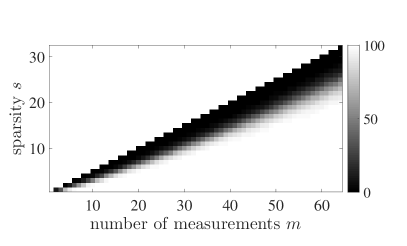
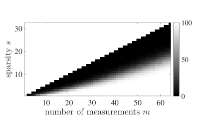
(a) $\mathbf{\Phi}\in\mathbb{H}^{m\times n}$

(b) $\mathbf{\Phi}\in\mathbb{R}^{m\times n}$

Figure 1: Results of the recovery experiment for $n=256$ and different $m$ and $s$. Image intensity stands for the percentage of perfect reconstructions.

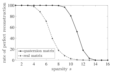
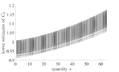
(a)

(b)

Figure 2: (a) Comparison of the recovery experiment results for $n=256$, $m=32$ and different values of $s$. (b) Lower estimate of the constant $C_{0}$ in Corollary 5.1 obtained from the inequality (5.2) for $n=256$ and $m=32$.

Fig. 1 (a) presents dependence of the perfect recovery percentage on the number of measurements $m$ and sparsity $s$ in the quaternion case. We see that simulations confirm our theoretical considerations. Fig. 1 (b) shows the same results for the real case, i.e. $\mathbf{\Phi}\in\mathbb{R}^{m\times n}$ and $\mathbbm{x}\in\mathbb{R}^{n}$. Note that in the first experiment for $m=32$ and $s\leq 9$ the recovery rate is greater than 95%, the same holds for $m=64$ and $s\leq 20$. It is also worth noticing that the results for coresponding pairs $(m,s)$ are much better in the quaternion setup than in the real-valued case (see Fig. 2(a)). We explain this phenomenon in [2, Lemma 3.1], namely, we show that for a fixed vector $\mathbbm{x}\in\mathbb{H}^{m}$ and the ensemble of quaternion Gaussian random matrices $\mathbf{\Phi}\in\mathbb{H}^{m\times n}$, the ratio random variable $\frac{\left\lVert{\mathbf{\Phi}\mathbbm{x}}\right\rVert_{2}^{2}}{\left\lVert{\mathbbm{x}}\right\rVert_{2}^{2}}$ has distribution $\Gamma(2m,2m)$, i.e. its variance equals $\frac{1}{2m}$, which is four times smaller than in the case of a real vector and real Gaussian matrices of the same size. In other words, a quaternion Gaussian random matrix statistically has smaller restricted isometry constant than its real counterpart.

We also performed another experiment illustrating the approximated reconstruction of non-sparse quaternion vectors from the exact data – as stated in Corollary 5.1. We fixed constants $n=256$ and $m=32$ and generated the measurement matrix $\mathbf{\Phi}\in\mathbb{H}^{m\times n}$ with random entries sampled from i.i.d. quaternion normal distribution and $1000$ arbitrary vectors $\mathbbm{x}\in\mathbb{H}^{n}$ with standard Gaussian random quaternion entries ($\sigma^{2}=1$), without assuming their sparsity. The above-described algorithm (steps 3.–6.) was applied to approximately reconstruct the vectors. We used the reconstruction errors $\left\lVert{\mathbbm{x}^{\#}-\mathbbm{x}}\right\rVert_{1}$ to obtain a lower bound on the constant $C_{0}$ as a function of $s$, for $s=1,\ldots,64$, using inequality (5.2), i.e.

$$C_{0}\geq\frac{\left\lVert{\mathbbm{x}^{\#}-\mathbbm{x}}\right\rVert_{1}}{\left\lVert{\mathbbm{x}-\mathbbm{x}_{s}}\right\rVert_{1}},$$

where $\mathbbm{x}_{s}$ denotes the best $s$-sparse approximation of $\mathbbm{x}$. The results of this experiment are shown in Fig. 2 (b) in the form of a scatter plot – each point represents a lower estimate of $C_{0}$ for one vector $\mathbbm{x}$ and sparsity $s$. We see in particular that – as expected – the dependence on $s$ is monotone.

7 Conclusions

The results of this article, together with aforementioned [2], form a theoretical background of the classical compressed sensing methods in the quaternion algebra. We extended the fundamental result of this theory to the full quaternion case, namely we proved that if a quaternion measurement matrix satisfies the RIP with a sufficiently small constant, then it is possible to reconstruct sparse quaternion signals from a small number of their measurements via $\ell_{1}$-norm minimization. We also estimated the error of the approximated reconstruction of a non-sparse quaternion signal from exact and noisy data. This improves our previous result for real measurement matrices and sparse quaternion vectors [1] and explains success of various numerical experiments in the quaternion setup [4, 17, 27].

There are several possibilities of further research in this field – both in theoretical and applied directions. Among others:
– further refinements of the main results in the quaternion algebra or their extensions to different algebraic structures,
– search for other than Gaussian quaternion matrices satisfying the RIP,
– adjust reconstruction algorithms to quaternions.
– applications of the theory in practice.
In view of numerous articles concerning quaternion signal processing published in the last decade, we expect that this new branch of compressed sensing will attract attention of even more researchers and considerably develop.

Acknowledgments

The research was supported in part by WUT grant No. 504/01861/1120. The work conducted by the second author was supported by a scholarship from Fundacja Wspierania Rozwoju Radiokomunikacji i Technik Multimedialnych.

References

[1] A. Badeńska, Ł. Błaszczyk, Compressed sensing for real measurements of quaternion signals, preprint (2015), arXiv:1605.07985.
[2] A. Badeńska, Ł. Błaszczyk, Quaternion Gaussian matrices satisfy the RIP, preprint (2017), arXiv:1704.08894.
[3] Q. Barthélemy, A. Larue, J. Mars, Sparse Approximations for Quaternionic Signals, Advances in Applied Clifford Algebras, 24 (2014), no. 2, 383–402.
[4] Q. Barthélemy, A. Larue, J. Mars, Color Sparse Representations for Image Processing: Review, Models, and Prospects, IEEE Trans Image Process, (2015), 1–12.
[5] T. Bülow, G. Sommer, Hypercomplex Signals – A Novel Extension of the Analytic Signal to the Multidimensional Case, IEEE Trans. Signal Processing, 49 (2001), no. 11, 2844–2852.
[6] T. Cai, A. Zhang, Sharp RIP bound for sparse signal and low-rank matrix recovery, Appl. Comput. Harmon. Anal. 35 (2013), no. 1, 74–93.
[7] E. J. Candès, The restricted isometry property and its implications for compressed sensing, C. R. Acad. Sci. Paris ser. I 346 (2008) 589-92.
[8] E. J. Candès, J. Romberg, T. Tao, Stable signal recovery from incomplete and inaccurate measurements, Comm. Pure Appl. Math. 59 (8) (2006) 1207–1223.
[9] E. J. Candès, T. Tao, Decoding by linear programming, IEEE Trans. Inform. Theory 51 (12) (2005) 4203–4215.
[10] W. L. Chan, H. Choi, R. G. Baraniuk, Coherent multiscale image processing using dual-tree quaternion wavelets, IEEE Trans. Image Process. 17 (2008), no. 7, 1069–1082.
[11] V. R. Dubey, Quaternion Fourier Transform for Colour Images, International Journal of Computer Science and Information Technologies, 5 (2014), no. 3, 4411–4416.
[12] T. A. Ell, S. J. Sangwine, Hypercomplex Fourier Transforms of Color Images, IEEE Trans. Image Process. 16 (2007), no. 1, 22–35.
[13] T. A. Ell, N. Le Bihan, S. J. Sangwine, Quaternion Fourier Transforms for Signal and Image Processing, Wiley-ISTE (2014).
[14] S. Foucart, H. Rauhut, A mathematical introduction to compressive sensing, Applied and Numerical Harmonic Analysis, Birkhäuser/Springer, New York (2013).
[15] N. Gomes, S. Hartmann, U. Kähler, Compressed Sensing for Quaternionic Signals, Complex Anal. Oper. Theory 11 (2017), 417–455.
[16] C. Gao, J. Zhou, F. Lang, Q. Pu, C. Liu, Novel Approach to Edge Detection of Color Image Based on Quaternion Fractional Directional Differentation, Advances in Automation and Robotics, 1 (2012) 163–170.
[17] M. B. Hawes, W. Liu, A Quaternion-Valued Reweighted Minimisation Approach to Sparse Vector Sensor Array Design, Proceedings of the 19th International Conference on Digital Signal Processing, (2014), 426–430.
[18] M. I. Khalil, Applying Quaternion Fourier Transforms for Enhancing Color Images, I.J. Image, Graphics and Signal Processing, 2 (2012), 9–15.
[19] S.-C. Pei, J.-H. Chang, J.-J. Ding, Color pattern recognition by quaternion correlation, IEEE Int. Conf. Image Process., Thessaloniki, Greece, October 7-10 (2010) 894–897.
[20] L. Rodman, Topics in Quaternion Linear Algebra, Princeton University Press, Princeton (2014).
[21] W. Rzadkowski, K. Snopek, A New Quaternion Color Image Watermarking Algorithm, The 8th IEEE International Conference on Intelligent Data Acquisition and Advanced Computing Systems: Technology and Applications, (2015), 245–250.
[22] K. M. Snopek, Quaternions and octonions in signal processing – fundamentals and some new results, Telecommunication Review + Telecommunication News, Tele-Radio-Electronic, Information Technology, 6 (2015), 618–622.
[23] J. F. Sturm, Using SeDuMi 1.02, A Matlab toolbox for optimization over symmetric cones, Optimization Methods and Software 11 (1999), no. 1-4, 625–653.
[24] C. C Took, D. P. Mandic, The Quaternion LMS Algorithm for Adaptive Filtering of Hypercomplex Processes, IEEE Trans. Signal Processing, 57(4) (2009) 1316–1327.
[25] N. N. Vakhania, G. Z. Chelidze, Quaternion Gaussian random variables, (Russian) Teor. Veroyatn. Primen. 54 (2009), no. 2, 337–344; translation in
Theory Probab. Appl. 54 (2010), no. 2, 363–369.
[26] B. Witten, J. Shragge, Quaternion-based Signal Processing, Stanford Exploration Project, New Orleans Annual Meeting (2006) 2862–2866.
[27] J. Wu, X. Zhang, X. Wang, L. Senhadji, H. Shu, L1-norm minimization for quaternion signals, Journal of Southeast University 1 (2013) 33–37.