Properties of blueshifted light rays in quasispherical Szekeres metrics

Abstract

This paper is a follow-up on two previous ones, in which properties of blueshifted rays were investigated in Lemaître – Tolman (L–T) and quasispherical Szekeres (QSS) spacetimes. In the present paper, an axially symmetric QSS deformation is superposed on such an L–T background that was proved, in the first paper, to mimic several properties of gamma-ray bursts. The present model makes $z$ closer to $-1$ than in the background L–T spacetime, and, as implied by the second paper, strong blueshifts exist in it only along two opposite directions. The QSS region is matched into a Friedmann background. The Big Bang (BB) function $t_{B}(r)$, which is constant in the Friedmann region, has a gate-shaped hump in the QSS region. Since a QSS island generates stronger blueshifts than an L–T island, the BB hump can be made lower – then it is further removed from the observer and implies a smaller observed angular radius of the source. Consequently, more sources can be fitted into the sky – all these facts are confirmed by numerical computations. Null geodesics reaching present observers from different directions relative to the BB hump are numerically calculated. Patterns of redshift across the image of the source and along the rays are displayed.

I Motivation and background

In Lemaître Lema1933 – Tolman Tolm1934 and Szekeres Szek1975 ; Szek1975b spacetimes, some of the light rays emitted at the Big Bang (BB) reach all observers with infinite blueshift ($1+z\ {\overset{\rm def}{=}}\ \nu_{e}/\nu_{o}=0$, where $\nu_{e}$ and $\nu_{o}$ are frequencies of the emitted and observed radiation, respectively). This is in contrast to Robertson – Walker spacetimes, where all light from the BB is observed with $z=\infty$ Elli1971 ; PlKr2006 . The quantity $z$, traditionally called redshift, being negative (and then called blueshift) means that the frequency observed is higher than the frequency at the emission point, and $z\to-1$ implies $\nu_{o}\to\infty$. The existence of blueshifts in L–T models was predicted by Szekeres in 1980 Szek1980 , in a casual remark without proof, and then confirmed by Hellaby and Lake in 1984 HeLa1984 by explicit calculation.

Two conditions are necessary for infinite blueshift:

(1) The BB time at the emission point of the ray must have nonzero spatial derivative in comoving-synchronous coordinates (the BB is “nonsimultaneous”).

(2) The ray is emitted at the BB in a radial direction.

Condition (2) was derived in Ref. HeLa1984 , but seems to have been overlooked by all later authors until Ref. Kras2016a , even though it follows quite simply from the geodesic equations. The two conditions together seem to be also sufficient, but a general proof of their sufficiency still does not exist; it is only implied by the full list of separate cases HeLa1984 and hinted at by numerical calculations Kras2016a ; Kras2014d .

The Szekeres spacetimes Szek1975 ; Szek1975b , in general, have no symmetry, thus no radial directions. In view of condition (2) it was not clear whether any rays with infinite blueshift exist in them. This question was addressed in Ref. Kras2016b . It was shown that in an axially symmetric quasispherical Szekeres (QSS) spacetime, $z=-1$ can possibly happen on axial rays; i.e., those that intersect every space of constant time on the symmetry axis. It was then confirmed by a numerical calculation in an exemplary QSS model that $1+z<10^{-5}$ along axial rays emitted from the BB. It was also shown, by a blind numerical search, that rays with $1+z<0.07$, and with similar spatial profiles of $z$ along neighbouring rays, exist in an exemplary fully nonsymmetric QSS model.

Since the L–T and Szekeres models have been proven to successfully describe several observed features of our Universe BoCK2011 ; SuGa2015 , and they predict a possible existence of blueshifts, one must thoroughly test the implications of blueshifts in order to either find a place for them among the observed phenomena, or conclude that the BB in the real Universe must have been simultaneous. With this motivation, it was shown in Ref. Kras2016a that an L–T region with a gate-shaped “hump” on the BB profile matched into a Friedmann background can mimic some observed properties of gamma-ray bursts (GRBs), such as the frequency range ($0.24\times 10^{19}$ to $1.25\times 10^{23}$ Hz), the existence of afterglows and the large distances to the sources. Placing several different L–T regions in the same Friedmann background would then account for the large number of possible sources. However, the model of Ref. Kras2016a was unsuccessful on two accounts:

(1) The gamma-ray flashes and the afterglows lasted for too long. The model contains a parameter that should allow for controlling the durations, but insufficient numerical accuracy did not permit actual use of it.

(2) The radiation was emitted isotropically instead of being collimated into narrow beams, as the observed GRBs are supposed to be Perlwww .

Also, the model of Ref. Kras2016a left some problems open. The main one was: how small could the humps on the BB profile be made while still generating the right range of frequencies of the observed radiation.

Ref. Kras2016b was the first step in improving the model of Ref. Kras2016a . It showed by examples that strongly blueshifted rays in QSS spacetimes exist only along two opposite directions. That paper also proved that in a QSS model the minimum $1+z$ is smaller than in an L–T model that has the same BB profile.

The present paper builds upon this last observation. The model considered here is a QSS deformation superposed on the L–T region of Ref. Kras2016a . Since the QSS deformation results in a smaller $1+z$ at the observer, the minimum value of $1+z$ found in Ref. Kras2016a can be achieved with a lower BB hump. This implies a greater distance between the source of radiation and the observer, and a smaller angular diameter of the source seen in the sky. The progress achieved with respect to Ref. Kras2016a is rather moderate, but this cannot be the ultimate limit of improvement: the class of BB profiles used here was found by trial and error (see Sec. XII), and it is impossible that the optimal shape could be hit upon in this way.

The L–T and Szekeres metrics are solutions of the Einstein equations with a dust source, so they cannot apply to the real Universe at such early times when pressure cannot be neglected. It is assumed that they may apply onward from the end of the last-scattering (LS) epoch. The mean mass density at LS, denoted $\rho_{\rm LS}$, in the now-standard $\Lambda$CDM model is known Kras2016a , see Sec. IV. For every past-directed null geodesic in a QSS (or L–T) region, the mass density at the running point is numerically calculated. When this density becomes equal to $\rho_{\rm LS}$, the integration is stopped. Thus, $1+z$ between LS and the present time is bounded from below, $z_{\rm LS}\geq z_{\rm min}>-1$. The computational problem is to arrange the BB profile so that it makes $z_{\rm LS}$ sufficiently near to $-1$ ($1+z_{\rm LS}<1.689\times 10^{-5}$ Kras2016a ), but does not lead to perturbations of the CMB radiation larger than observations allow. Among other things, this implies that the model must be capable of making the angular diameter of the radiation sources smaller than the observed diameter of the GRBs (currently $\approx 1^{\circ}$, see Sec. XI).

In Secs. II and III, the subfamily of QSS models employed here is presented. It is an axially symmetric QSS region matched into a Friedmann background with curvature index $k=-0.4$. In Sec. IV the parameters of the background model are specified. They are different from those of the $\Lambda$CDM model Plan2014 ; Plan2014b – it was convenient to keep them the same as in the earlier papers by this author Kras2016a ; Kras2014d . In Sec. V, the equations of null geodesics in the QSS region are presented. In Sec. VI, basic properties of redshift are described, and the conditions for $z=-1$ in an axially symmetric QSS model are spelled out. In Sec. VII, the equation of the Extremum Redshift Surface (ERS) is derived, on which $z$ has maxima or minima along axial rays. In Sec. VIII, the numerical parameters of the model used here are adapted to the GRBs of lowest frequency. In Sec. IX, exemplary nonaxial plane rays reaching the present observers are numerically determined. The observers are placed in three directions with respect to the QSS region: (I) – in prolongation of the dipole minimum, (II) – in prolongation of the dipole maximum, and (III) – in prolongation of the dipole equator of the boundary of the QSS region. For each observer, the redshift profiles across the image of the radiation source are presented in tables. In Sec. X, redshift profiles along the nonaxial rays reaching Observer I are displayed to show that analogues of the ERS exist also along nonaxial directions. In Sec. XI it is estimated that $\approx 11,000$ radiation sources of Sec. VIII could be fitted into the celestial sphere. The necessary and possible improvements of the model are discussed in Sec. XII. Section XIII contains the summary and conclusions.

The present paper is a study in the geometry of the QSS spacetimes and in properties of their blueshifted rays. Also, it introduces methods that can be used in further refinements of the model. The observed parameters of the GRBs were used as a beacon pointing the way, but the configuration derived here needs further improvements before it can be considered a model of a GRB source; see Sec. XI.

Most results of numerical calculations are quoted up to 17 decimal digits. Such precision is needed to capture time intervals of $\approx 10$ min at the observer, which is $\approx 2\times 10^{-16}$ in the units used here, see Sec. III. (The 10 min is a representative time during which GRBs are visible to the detectors Kras2016a .)

II QSS spacetimes

The metric of the QSS spacetimes is Szek1975 ; Szek1975b ; PlKr2006 ; Hell1996

$${\rm d}s^{2}={\rm d}t^{2}-\frac{\left(\Phi,_{r}-\Phi{\cal E},_{r}/{\cal E}\right)^{2}}{1+2E(r)}{\rm d}r^{2}-\left(\frac{\Phi}{\cal E}\right)^{2}\left({\rm d}x^{2}+{\rm d}y^{2}\right),\ \ \ \ \$$ (1)

$${\cal E}\ {\overset{\rm def}{=}}\ \frac{S}{2}\left[\left(\frac{x-P}{S}\right)^{2}+\left(\frac{y-Q}{S}\right)^{2}+1\right],$$ (2)

$P(r)$, $Q(r)$, $S(r)$ and $E(r)$ being arbitrary functions such that $S\neq 0$ and $E\geq-1/2$ at all $r$.

The source in the Einstein equations is dust ($p=0$) with the velocity field $u^{\alpha}={\delta_{0}}^{\alpha}$. The surfaces of constant $t$ and $r$ are nonconcentric spheres, and $(x,y)$ are stereographic coordinates on each sphere. At a fixed $r$, they are related to the spherical coordinates by

$$x = P+S\cot(\vartheta/2)\cos\varphi,$$

$$y = Q+S\cot(\vartheta/2)\sin\varphi.$$ (3)

The functions $(P,Q,S)$ determine the centers of the spheres in the spaces of constant $t$ (see illustrations in Ref. Kras2016b ). Because of the nonconcentricity, the QSS spacetimes, in general, have no symmetry BoST1977 .

With $\Lambda=0$ assumed, $\Phi(t,r)$ obeys

$${\Phi,_{t}}^{2}=2E(r)+\frac{2M(r)}{\Phi},$$ (4)

where $M(r)$ is an arbitrary function. We consider models with $E>0$, then

$$\Phi(t,r) = \frac{M}{2E}(\cosh\eta-1),$$

$$\sinh\eta-\eta = \frac{(2E)^{3/2}}{M}\left[t-t_{B}(r)\right],$$ (5)

where $t_{B}(r)$ is one more arbitrary function; $t=t_{B}(r)$ is the BB time, at which $\Phi(t_{B},r)=0$. We assume $\Phi,_{t}>0$ (the Universe is expanding).

The mass density implied by (1) is

$$\kappa\rho=\frac{2\left(M,_{r}-3M{\cal E},_{r}/{\cal E}\right)}{\Phi^{2}\left(\Phi,_{r}-\Phi{\cal E},_{r}/{\cal E}\right)},\quad\kappa\ {\overset{\rm def}{=}}\ \frac{8\pi G}{c^{2}}.$$ (6)

This density distribution is a mass dipole superposed on a spherically symmetric monopole Szek1975b ; DeSo1985 . The dipole, generated by ${\cal E},_{r}/{\cal E}$, vanishes where ${\cal E},_{r}=0$. The density is minimum where ${\cal E},_{r}/{\cal E}$ is maximum and vice versa HeKr2002 .

The arbitrary functions must be such that $0<\rho<\infty$ at all $t>t_{B}(r)$. The conditions that ensure this are HeKr2002 :

$$\frac{M,_{r}}{3M} \geq \frac{\sqrt{(S,_{r})^{2}+(P,_{r})^{2}+(Q,_{r})^{2}}}{S}~{}~{}~{}~{}\forall~{}r,$$ (7)

$$\frac{E,_{r}}{2E} > \frac{\sqrt{(S,_{r})^{2}+(P,_{r})^{2}+(Q,_{r})^{2}}}{S}~{}~{}~{}~{}\forall~{}r.$$ (8)

These inequalities imply HeKr2002

$$\frac{M,_{r}}{3M}\geq\frac{{\cal E},_{r}}{\cal E},\qquad\frac{E,_{r}}{2E}>\frac{{\cal E},_{r}}{\cal E}\qquad\forall~{}r.$$ (9)

The extrema of ${\cal E},_{r}/{\cal E}$ with respect to $(x,y)$ are HeKr2002

$$\left.\frac{{\cal E},_{r}}{\cal E}\right|_{\rm extreme}=\pm\frac{\sqrt{(S,_{r})^{2}+(P,_{r})^{2}+(Q,_{r})^{2}}}{S},$$ (10)

with $+$ corresponding to maximum and $-$ to minimum. In the following, we will call these two loci “dipole maximum” and “dipole minimum”, respectively.

The L–T models follow from the QSS models as the limit of constant $(P,Q,S)$. Then the constant-$(t,r)$ spheres become concentric, and the spacetime becomes spherically symmetric. The Friedmann limit is obtained when $E/M^{2/3}$ and $t_{B}$ are constant (in this limit, $(P,Q,S)$ can be made constant by a coordinate transformation). A QSS spacetime can be matched to a Friedmann spacetime across an $r=$ constant hypersurface.

Because of $p=0$, the QSS models can describe the past evolution of the Universe no further back than to the last scattering hypersurface (LSH). See Sec. VIII for information on how to determine it in our model.

III The QSS models considered in this paper

We will consider such QSS spacetimes whose L–T limit is Model 2 of Ref. Kras2016a . The $r$-coordinate is chosen so that

$$M=M_{0}r^{3},$$ (11)

and $M_{0}=1$ (kept in formulae for dimensional clarity) Kras2014d . From this point on, the $r$-coordinate is unique. The function $E(r)$, assumed in the form

$$2E/r^{2}\ {\overset{\rm def}{=}}\ -k=0.4,$$ (12)

is the same as in the background Friedmann model.

The units used in numerical calculations were introduced and justified in Ref. Kras2014a . Taking unitconver

$$1\ {\rm pc}=3.086\times 10^{13}\ {\rm km},\quad 1\ {\rm y}=3.156\times 10^{7}\ {\rm s},$$ (13)

the numerical length unit (NLU) and the numerical time unit (NTU) are defined as follows:

$$1\ {\rm NTU}=1\ {\rm NLU}=9.8\times 10^{10}\ {\rm y}=3\times 10^{4}\ {\rm Mpc}.$$ (14)

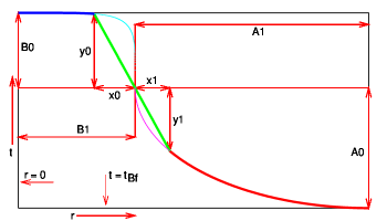
Figure 1: Parameters of the bang-time profile in the quasispherical Szekeres region; see text for explanation.

The BB profile belongs to the same 5-parameter family as in Ref. Kras2016a , see Fig. 1. It consists of two curved arcs and a straight line segment joining them. The upper-left arc, shown as a thicker line, is a segment of the curve

$$\frac{r^{6}}{{B_{1}}^{6}}+\frac{\left(t-t_{\rm Bf}-A_{0}\right)^{6}}{{B_{0}}^{6}}=1,$$ (15)

where

$$t_{\rm Bf}=-0.13945554689046649\ {\rm NTU}\approx-13.67\times 10^{9}\ {\rm years};$$ (16)

see Sec. IV for comments on this value. The lower-right arc (also shown as a thicker line) is a segment of the ellipse

$$\frac{\left(r-B_{1}-A_{1}\right)^{2}}{{A_{1}}^{2}}+\frac{\left(t-t_{\rm Bf}-A_{0}\right)^{2}}{{A_{0}}^{2}}=1.$$ (17)

The straight segment passes through the point $(r,t)=(B_{1},t_{\rm Bf}+A_{0})$ where the full curves (shown as dotted lines) would meet; $x_{0}$ determines its slope.

The free parameters are $A_{0}$, $A_{1}$, $B_{0}$, $B_{1}$ and $x_{0}$. Figure 1 does not show the values used in numerical calculations; in particular $x_{0}$ and $A_{1}$ are greatly exaggerated. The actual values in Model 2 of Ref. Kras2016a are

$$\left(\begin{array}[]{l}A_{0}\\ B_{0}\\ A_{1}\\ B_{1}\\ x_{0}\\ \end{array}\right)=\left(\begin{array}[]{l}0.000026\ {\rm NTU}\\ 0.0001\ {\rm NTU}\\ 1\times 10^{-10}\\ 0.015\\ 2\times 10^{-13}\\ \end{array}\right)$$ (18)

($A_{1}$, $B_{1}$ and $x_{0}$ are dimensionless). This profile will be the starting point for modifications.

The QSS model used here is axially symmetric, with $P(r)=Q(r)=0$ and $S(r)$ the same as in Ref. Kras2016b :

$$S=\sqrt{a^{2}+r^{2}},$$ (19)

where $a>0$ is a constant, and so

$${\cal E}=\frac{1}{2S}\ \left(x^{2}+y^{2}+S^{2}\right);$$ (20)

This $S(r)$ obeys (7) and (8), which, using (11) and (12), both reduce to

$$1/r>S,_{r}/S.$$ (21)

The equation of the dipole “equator” ${\cal E},_{r}=0$ is

$$x^{2}+y^{2}=S^{2};$$ (22)

the axis of symmetry is $x=y=0$. The extrema of the dipole are, from (10)

$$\left.\frac{{\cal E},_{r}}{\cal E}\right|_{\rm extreme}=\pm\frac{S,_{r}}{S}.$$ (23)

At $r>r_{b}$, where

$$r_{b}=A_{1}+B_{1}=0.0150000001,$$ (24)

the BB profile becomes flat, and the geometry of the model becomes Friedmannian. See Sec. V for remarks on the choice of coordinates in that region.

IV The background model

Our Friedmann background is defined by:

$$\Lambda=0,\qquad k=-0.4,\qquad t_{B}=t_{\rm Bf},$$ (1)

where $k$ is the curvature index and $t_{B}$ is the BB time given by (16); $t=0$ is the present time. The $t_{\rm Bf}$ is the asymptotic value of the function $t_{B}(r)$ in the L–T model that mimicked accelerating expansion Kras2014d . This differs by $\sim 1.6\%$ from $(-T)$, where $T$ is the age of the Universe given by the Planck satellite team Plan2014

$$T=13.819\times 10^{9}\ {\rm y}=0.141\ {\rm NTU}.$$ (2)

The density at the last scattering time is Kras2016a

$$\kappa\rho_{\rm LS}=56.1294161975316\times 10^{9}\ ({\rm NLU})^{-2}.$$ (3)

This value follows from the model of the cosmological recombination process Peeb1968 ; ZKSu1968 ; recoWiki and is independent of the after-recombination model. With (1), $\rho_{\rm LS}$ implies the redshift relative to the present time

$$1+z^{\rm b}_{\rm LS}=952.611615159.$$ (4)

This differs by $\sim 12.7\%$ from the $\Lambda$CDM value Plan2014 ; Plan2014b

$$z_{\rm LS}=1090.$$ (5)

The present temperature of the CMB radiation is directly measured, so if (4) were taken for real, the temperature of the background radiation at emission would be $\sim 3380$ K instead of $\sim 3000$ K dictated by current knowledge. To reconcile our model with these data, many recalculations would be required. Since our model needs other improvements anyway, we will stick to (1), to be able to compare the present results with the earlier ones.

V Null geodesics in the axially symmetric QSS spacetimes

In an axially symmetric QSS metric, $x$ and $y$ can be chosen such that $P=Q=0$; then $x=y=0$ is the symmetry axis BKHC2010 ; NoDe2007 . However, the loci $x=\infty$ and $y=\infty$ are coordinate singularities (they are at the pole of the stereographic projection), and numerical integration of nonaxial geodesics breaks down on crossing those sets. Therefore, we introduce the new coordinates $(\vartheta,\varphi)$ by

$$x=S_{b}\cot(\vartheta/2)\cos\varphi,\qquad y=S_{b}\cot(\vartheta/2)\sin\varphi,$$ (1)

where $S_{b}$ is $S$ at the Szekeres/Friedmann boundary:

$$S_{b}\ {\overset{\rm def}{=}}\ S(r_{b})=\sqrt{a^{2}+{r_{b}}^{2}}.$$ (2)

This changes (1) and (2) to

$${\rm d}s^{2}={\rm d}t^{2}-\frac{{\cal N}^{2}{\rm d}r^{2}}{1+2E(r)}-\left(\frac{\Phi}{\cal F}\right)^{2}\left({\rm d}\vartheta^{2}+\sin^{2}\vartheta{\rm d}\varphi^{2}\right),\\$$ (3)

$${\cal F} \ {\overset{\rm def}{=}}\ \frac{S_{b}}{2S}\ (1+\cos\vartheta)+\frac{S}{2S_{b}}\ (1-\cos\vartheta),$$

$${\cal N} \ {\overset{\rm def}{=}}\ \Phi,_{r}-\Phi{\cal F},_{r}/{\cal F}.$$ (4)

The dipole equator ${\cal F},_{r}=0$ is now at $\cot(\vartheta_{\rm eq}/2)=S/S_{b}$ (so $\vartheta_{\rm eq}=\pi/2$ at the QSS boundary). On the boundary sphere $r=r_{b}$ we have ${\cal F}=1$ and $(\vartheta,\varphi)$ become the spherical coordinates with the origin at $r=0$.

Along a geodesic we denote

$$\left(k^{t},k^{r},k^{\vartheta},k^{\varphi}\right)\ {\overset{\rm def}{=}}\ \frac{{\rm d}{(t,r,\vartheta,\varphi)}}{{\rm d}{\lambda}},$$ (5)

where $\lambda$ is an affine parameter. The geodesic equations for (3) – (4) are

$$\frac{{\rm d}{k^{t}}}{{\rm d}{\lambda}}+\frac{{\cal N}{\cal N},_{t}}{1+2E}\left(k^{r}\right)^{2}+\frac{\Phi{\Phi,_{t}}}{{\cal F}^{2}}\left[\left(k^{\vartheta}\right)^{2}+\sin^{2}\vartheta\left(k^{\varphi}\right)^{2}\right]=0,$$ (6)

$$\frac{{\rm d}{k^{r}}}{{\rm d}{\lambda}} + 2\frac{{\cal N},_{t}}{\cal N}k^{t}k^{r}$$ (7)

$$+ \left(\frac{{\cal N},_{r}}{\cal N}-\frac{E,_{r}}{1+2E}\right)\left(k^{r}\right)^{2}+2\frac{S,_{r}\sin\vartheta\Phi}{S{\cal F}^{2}{\cal N}}\ k^{r}k^{\vartheta}$$

$$- \frac{\Phi(1+2E)}{{\cal F}^{2}{\cal N}}\left[\left(k^{\vartheta}\right)^{2}+\sin^{2}\vartheta\left(k^{\varphi}\right)^{2}\right]=0,$$

$$\frac{{\rm d}{k^{\vartheta}}}{{\rm d}{\lambda}} + 2\frac{\Phi,_{t}}{\Phi}k^{t}k^{\vartheta}-\frac{S,_{r}\sin\vartheta{\cal N}}{S\Phi(1+2E)}\ \left(k^{r}\right)^{2}+2\frac{\cal N}{\Phi}k^{r}k^{\vartheta}$$ (8)

$$+ \frac{{\cal F},_{\vartheta}}{\cal F}\ \left[-\left(k^{\vartheta}\right)^{2}+\sin^{2}\vartheta\left(k^{\varphi}\right)^{2}\right]$$

$$- \cos\vartheta\sin\vartheta\left(k^{\varphi}\right)^{2}=0,$$

$$\frac{{\rm d}{k^{\varphi}}}{{\rm d}{\lambda}} + 2\frac{\Phi,_{t}}{\Phi}k^{t}k^{\varphi}+2\frac{\cal N}{\Phi}k^{r}k^{\varphi}$$ (9)

$$+ 2\left[\frac{\cos\vartheta}{\sin\vartheta}-\frac{{\cal F},_{\vartheta}}{\cal F}\right]k^{\vartheta}k^{\varphi}=0.$$

The geodesics determined by (6) – (9) are null when

$$\left(k^{t}\right)^{2}-\frac{{\cal N}^{2}\left(k^{r}\right)^{2}}{1+2E(r)}-\left(\frac{\Phi}{\cal F}\right)^{2}\left[\left(k^{\vartheta}\right)^{2}+\sin^{2}\vartheta\left(k^{\varphi}\right)^{2}\right]=0.$$ (10)

Note that $k^{\varphi}\equiv 0$ is a solution of (9) while $\vartheta\equiv 0$ and $\vartheta\equiv\pi$ (axial rays) are solutions of (8).

To calculate $k^{r}$ on nonaxial null geodesics, Eq. (10) will be used, which is insensitive to the sign of $k^{r}$. A numerical program for integrating the set {(6), (8) – (10)} will have to change the sign of $k^{r}$ wherever $k^{r}$ reaches zero.

There exist no null geodesics on which $k^{\varphi}\equiv 0$ and $\vartheta$ has any constant value other than 0 or $\pi$. This follows from (8): Suppose $k^{\varphi}\equiv 0$ everywhere and $k^{\vartheta}=0$ at a point. Then, if $\sin\vartheta\neq 0$, the third term in (8) will be nonzero (because $\left|S\Phi(1+2E)\right|<\infty$, $S,_{r}\neq 0$ from (19), ${\cal N}\neq 0$ from no-shell-crossing conditions HeKr2002 and $k^{r}\neq 0$ from (10)), and so ${{\rm d}{k^{\vartheta}}}/{{\rm d}{\lambda}}\neq 0$. Consequently, in the axially symmetric case the only analogues of radial directions are $\vartheta=0$ and $\vartheta=\pi$. The fact reported under (4) below is consistent with this.

The coefficient $1/\Phi$ in (8) and (9) becomes infinite at $r=0$, where $\Phi=0$ Kras2016a , but all the suspicious-looking terms are in fact finite there Kras2016b . In the present paper the only geodesics running through $r=0$ will be the axial ones, on which (8) and (9) are obeyed identically.

Let the subscript $o$ refer to the observation point. On past-directed rays $k^{t}<0$ and the affine parameter along each one can be chosen such that

$$k^{t}_{o}=-1.$$ (11)

Then, from (10) we have

$$\left(k_{o}^{\vartheta}\right)^{2}+\sin^{2}\vartheta\left(k_{o}^{\varphi}\right)^{2}\leq\left(\frac{{\cal F}_{o}}{\Phi_{o}}\right)^{2};$$ (12)

the equality occurs when the ray is tangent to a hypersurface of constant $r$ at the observation event, $k_{o}^{r}=0$.

On the boundary $r=r_{b}$ between the QSS and Friedmann regions the coordinates on both sides must coincide. Thus, for the Friedmann region one must use the metric (3) with $t_{B}=t_{\rm Bf}$ given by (16) ($E$ has the Friedmann form (12) everywhere). The metric then becomes Friedmann with no further limitation on $S$. But for correspondence with Ref. Kras2016a , we choose the coordinates in the Friedmann region so that

$$S=\sqrt{a^{2}+{r_{b}}^{2}}=S_{b}.$$ (13)

Then, ${\cal F}=1$ and $(\vartheta,\varphi)$ are the spherical coordinates throughout the Friedmann region.

VI The redshift in axially symmetric QSS spacetimes

Along a ray emitted at $P_{e}$ and observed at $P_{o}$

$$1+z=\frac{\left(u_{\alpha}k^{\alpha}\right)_{e}}{\left(u_{\alpha}k^{\alpha}\right)_{o}},$$ (1)

where $u_{\alpha}$ are the four-velocities of the emitter and of the observer, and $k^{\alpha}$ is the affinely parametrised tangent vector field to the ray Elli1971 . In our case, both $u_{\alpha}={\delta^{0}}_{\alpha}$, and then (1) simplifies to $1+z={k_{e}}^{t}/{k_{o}}^{t}$. If the affine parameter is rescaled so that (11) holds, then

$$1+z=-{k_{e}}^{t}.$$ (2)

Equation (9) has the first integral:

$$k^{\varphi}\sin^{2}\vartheta\Phi^{2}/{\cal F}^{2}=J_{0},$$ (3)

where $J_{0}$ is constant. When (3) is substituted in (10), the following results:

$$(k^{t})^{2}=\frac{{\cal N}^{2}\left(k^{r}\right)^{2}}{1+2E}+\left(\frac{\Phi}{\cal F}\right)^{2}\left(k^{\vartheta}\right)^{2}+\left(\frac{J_{0}{\cal F}}{\sin\vartheta\Phi}\right)^{2}.$$ (4)

Equations (4) and (2) show that for rays emitted at the BB, where $\Phi=0$, the observed redshift is infinite when $J_{0}\neq 0$. A necessary condition for infinite blueshift ($1+z_{o}=0$) is thus $J_{0}=0$, so

(a) either $k^{\varphi}=0$, i.e. the ray proceeds in the hypersurface of constant $\varphi$,

(b) or $\vartheta=0,\pi$ along the ray ($J_{0}/\sin\vartheta\to 0$ when $\vartheta\to 0,\pi$ by (3)).

Condition (b) appears to be also sufficient, but this has been demonstrated only numerically in concrete examples of QSS models (Kras2016b and Sec. VIII here).

Consider a ray proceeding from event $P_{1}$ to $P_{2}$ and then from $P_{2}$ to $P_{3}$. Denote the redshifts acquired in the intervals $[P_{1},P_{2}]$, $[P_{2},P_{3}]$ and $[P_{1},P_{3}]=[P_{1},P_{2}]\cup[P_{2},P_{3}]$ by $z_{12}$, $z_{23}$ and $z_{13}$, respectively. Then, from (1)

$$1+z_{13}=\left(1+z_{12}\right)\left(1+z_{23}\right).$$ (5)

In particular, for a ray proceeding to the past from $P_{1}$ to $P_{2}$, and then back to the future from $P_{2}$ to $P_{1}$:

$$1+z_{12}=\frac{1}{1+z_{21}}.$$ (6)

VII The Extremum Redshift Surface

Consider a null geodesic that stays in the surface $\{\vartheta,\varphi\}=\{\pi,{\rm constant}\}$; it obeys (8) and (9) identically. On it, $k^{r}\neq 0$ at all points because with $k^{\vartheta}=k^{\varphi}=0$ the geodesic would be timelike wherever $k^{r}=0$, so $r$ can be used as a parameter. Assume the geodesic is past-directed so that (2) applies. Using (2) and changing the parameter to $r$, we obtain from (6)

$$\frac{{\rm d}{z}}{{\rm d}{r}}=\frac{{\cal N}{\cal N},_{t}}{1+2E}\ k^{r}.$$ (1)

Since ${\cal N}\neq 0$ from no-shell-crossing conditions HeKr2002 and $k^{r}\neq 0$, the extrema of $z$ on such a geodesic occur where

$${\cal N},_{t}\equiv\Phi,_{tr}-\Phi,_{t}{\cal F},_{r}/{\cal F}=0.$$ (2)

In deriving (2), $\vartheta=\pi$ was assumed, but $\varphi$ was an arbitrary constant. Thus, the set in spacetime defined by (2) is 2-dimensional; it is the Extremum Redshift Surface (ERS) Kras2016b .

From (4) and (12) we obtain

$$\Phi,_{t} = r\sqrt{\frac{2M_{0}r}{\Phi}-k},$$ (3)

$$\Phi,_{tr} = \sqrt{\frac{2M_{0}r}{\Phi}-k}+\frac{M_{0}r^{3}}{\Phi^{2}}\ t_{B,r}.$$ (4)

Using (3), (4) and (4) with $\vartheta=\pi$, Eq. (2) becomes

$$\sqrt{\frac{2M_{0}r}{\Phi}-k}\left(1-r\frac{S,_{r}}{S}\right)=-\frac{M_{0}r^{3}}{\Phi^{2}}\ t_{B,r}.$$ (5)

To avoid shell crossings, $t_{B,r}<0$ must hold at all $r>0$ HeKr2002 , PlKr2006 , so the right-hand side of (5) is non-negative. The left-hand side is positive with $S$ given by (19). Using (II) for $\Phi$, remembering that $k<0$ and denoting

$$\chi\ {\overset{\rm def}{=}}\ \sinh^{2}(\eta/2)$$ (6)

we obtain from (5)

$$\chi^{4}+\chi^{3}=-k^{3}\left[\frac{rt_{B,r}}{4M_{0}\left(1-rS,_{r}/S\right)}\right]^{2}.$$ (7)

With $k<0$, (7) is solvable for $\chi$ at any $r$, since its left-hand side is independent of $r$ and can vary from 0 to $+\infty$ while the right-hand side is non-negative.

Note that where $t_{B,r}=0$, Eqs. (7) and (6) imply $\chi=\eta=0$, i.e. at those points the ERS is tangent to the BB. Also, the ERS is tangent to the BB at $r=0$ unless ${{\rm d}{t_{B}}}/{{\rm d}{r}}\ {\underset{r\to 0}{\longrightarrow}}\ \infty$. (This would imply ${{\rm d}{\rho}}/{{\rm d}{r}}\ {\underset{r\to 0}{\longrightarrow}}\ \infty$, an infinitely thin peak in density at $r=0$ – an unusual configuration, but not a curvature singularity KHBC2010 .) The model considered here will have $t_{B,r}=0$ at $r=0$.

In the limit $S,_{r}=0$, (7) reproduces the equation of the Extremum Redshift Hypersurface (ERH) of Ref. Kras2014d .

Equation (7) was derived for null geodesics proceeding along $\vartheta=\pi$, where ${\cal F},_{r}/{\cal F}=S,_{r}/S>0$. With $S$ given by (19) we have

$$F_{1}\ {\overset{\rm def}{=}}\ 1/\left(1-rS,_{r}/S\right)=(r/a)^{2}+1>1,$$ (8)

so, at a given $r$, the ERS has a greater $\eta$ (and so a greater $t-t_{B}$) than the corresponding ERH of the L–T model. Also, the extrema of $z$ along the dipole maximum occur at a greater $\chi$ (and thus greater $t-t_{B}$) when $a$ is smaller. This will be illustrated by Fig. 2 in the next section.

Conversely, for a ray proceeding along the dipole minimum axis (where $\vartheta=0$), the factor $F_{1}$ is replaced by

$$F_{2}\ {\overset{\rm def}{=}}\ 1/\left(1+rS,_{r}/S\right)=\frac{a^{2}+r^{2}}{a^{2}+2r^{2}}<1,$$ (9)

and so the ERS has a smaller $t-t_{B}$ than the ERH in L–T. Also here, a smaller $a$ has a more pronounced effect.

Extrema of redshift also exist along directions other than $\vartheta=0$ and $\vartheta=\pi$, as will be demonstrated by numerical examples in Sec. X, but a general equation defining their loci remains to be derived.

VIII A generalised Model 2 of Ref. Kras2016a

Along each past-directed null geodesic, the mass density is calculated using (II) – (6). As explained in Sec. IV, in any model the density at the LSH must be the same as in (3). So, the instant of crossing the LSH is that where the density becomes equal to (3).

The starting point for this paper is Model 2 of Ref. Kras2016a , whose functions $M(r)$, $E(r)$ and $t_{B}(r)$ are given by (11), (12) and (15) – (18). In that model, the strongest blueshift between the LSH and the present epoch was

$$1+z_{\rm maxb}=1.36167578\times 10^{-5}.$$ (1)

It was calculated by the rule (5). The first factor,

$$1+z_{\rm ols2}=1.07858890707746014\times 10^{-7},$$ (2)

was the blueshift between the LSH and $r=0$, achieved on a path that will be called “Ray A”. The second factor,

$$1+z_{\rm po2}=126.246039921.$$ (3)

was the redshift between $r=0$ and the present epoch on a path going off from the same initial point as Ray A, but to the future; it will be called “Ray B”.

On Model 2, axially symmetric QSS deformations given by $P=Q=0$, (19) and (20) are superposed. Numerical experiments with rays proceeding along $\vartheta=\pi$ were done to improve on (1) as much as possible. As explained under (8), smaller $a$ increases the region under the ERS. So, with the parameters of (18), $a^{2}$ was gradually changed from 10 through 1, 1/10, $10^{-2}$, $10^{-3}$ to $10^{-4}$. For each $a$ the quantity

$$t(0)-t_{B}(0)\ {\overset{\rm def}{=}}\ \Delta t_{c}$$ (4)

was chosen such as to obtain a minimum $1+z$ between the LSH and $r=0$. This led to smaller $1+z$ on Ray A only down to $a^{2}=0.001$. With $a^{2}$ still smaller, the ray either flew over the BB hump and crossed the LSH in the Friedmann region with a large $z>0$ or dipped under the LSH still within the QSS region with a small $z>0$. No intermediate value of $\Delta t_{c}$ led to $z<0$ (but this discontinuity could possibly be overcome with greater numerical precision). The best result achieved with $a^{2}=0.001$ was $1+z_{2}=8.87933914173189009\times 10^{-8}$.

In the next experiments, the slope of the straight segment of the BB profile was gradually decreased, i.e $x_{0}$ was increased from $2\times 10^{-13}$ through $1\times 10^{-12}$ to $1\times 10^{-11}$, with the other parameters unchanged. For each value of $x_{0}$, the $\Delta t_{c}$ leading to the smallest $1+z$ was determined. The best result achieved at this stage was

$$1+z_{1}=6.74014204449235876\times 10^{-8}.$$ (5)

Varying $A_{1}$, $B_{1}$, $B_{0}$, and lowering the degree of (15) to 4 and to 2, led to nothing better than (5). So, this is taken as the best improvement over the L–T model achieved using an axially symmetric QSS deformation.

Figure 2 shows Ray A, with $1+z_{1}$ given by (5), and the corresponding ERS and BB profiles. Curve 1 is the ERH profile of Model 2 from Ref. Kras2016a , and Curve 2 is the ERS profile with $a^{2}=10^{-5}$. As stated above, smaller $a$ gives more space under the ERS, but when too small it creates a discontinuity in $z$ that prevents $z<0$ altogether.

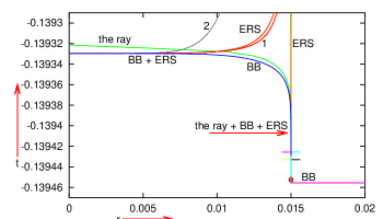
Figure 2: The Big Bang profile and the axial ray with the smallest $1+z$ in the Szekeres model. The short horizontal strokes are at the ends of the straight BB segment. The dot shows where the ray hits the LSH. See text for more explanation.

The ERS profile has two branches on each side of $r=0$, so some rays will intersect it four times and $z$ along them will have two local maxima and two local minima. Examples will appear in Sec. X.

On Ray B, the upward $1+z$ is

$$1+z_{\rm 1\ up}=6.39228356761256666\times 10^{-3}.$$ (6)

Thus, total $(1+z)$ between LSH and now is

$$1+z_{2}=\frac{1+z_{1}}{1+z_{\rm 1\ up}}=1.05441849899\times 10^{-5}\ \ \ \ .$$ (7)

This fits the lowest-frequency GRBs, for which Kras2016a

$$1+z_{\rm max}\approx 1.689\times 10^{-5},$$ (8)

with a wider margin than (1), so the BB hump can now be lowered to yield $(1+z)$ closer to (8). The easiest way to do this is to decrease $B_{0}$ (see Fig. 1). Then $\Delta t_{c}$ is fine-tuned to make $(1+z_{\rm ols})$ on Ray A as small as possible ($1+z_{\rm ols}$ gets larger when $B_{0}$ gets smaller, so there is a limit on decreasing $B_{0}$). The $B_{0}$ that allows sufficiently small $(1+z)_{\rm ols}$ is

$$B_{0}=0.000091,$$ (9)

and then the smallest $1+z$ on Ray A is

$$1+z_{\rm ols3}=1.11939135405414447\times 10^{-7}.$$ (10)

For Ray B corresponding to Ray A of (10) (proceeding along the dipole minimum), the $1+z$ between $r=0$ and the present epoch is

$$1+z_{\rm 3\ up}=7.11151887923544557\times 10^{-3},$$ (11)

so $(1+z)$ between LSH and now along Rays A and B is

$$1+z_{3}=\frac{1+z_{\rm ols3}}{1+z_{\rm 3\ up}}=1.574\times 10^{-5},$$ (12)

and the present observer is at

$$r=r_{\rm obs}=0.88983013520392229.$$ (13)

This is larger than $r_{\rm O2}=0.88705643159726955$ in Model 2 of Ref. Kras2016a . Thus, a Szekeres deformation superposed on an L–T model results in moving the observer further from the radiation source, which leads to a smaller angular diameter of the source seen in the sky; see Sec. IX.

Rays A and B referred to above have

$$\Delta t_{c}=0.00000863099500\ {\rm NTU}.$$ (14)

The corresponding results for rays propagating in the opposite direction, i.e. along the dipole minimum between the LSH and $r=0$ (Ray C), and along the dipole maximum between $r=0$ and the observer (Ray D), are as follows. The best value of $1+z$ on Ray C is

$$1+z_{\rm 1\ dip\ min}=1.73185662921682137\times 10^{-7},$$ (15)

achieved with

$$\Delta t_{c}=0.00000981550000\ {\rm NTU}.$$ (16)

Then, $1+z$ calculated toward the future along the dipole maximum is

$$1+z_{\rm 2\ dmax\ up}=7.26948511585012724\times 10^{-3}.$$ (17)

So, the $1+z$ between the LSH and the present time is

$$1+z_{4}=\frac{1+z_{\rm 1\ dip\ min}}{1+z_{\rm 2\ dmax\ up}}=2.382\times 10^{-5}.$$ (18)

The present time was reached by the ray at

$$\widetilde{r}_{\rm obs}=0.88935629118490100.$$ (19)

Thus, on this ray $1+z$ is larger while $r_{\rm obs}$ is smaller.

In each case the numerical calculation overshot the present time. For the ray that produced (11) and (13), the value of $t$ at the endpoint was

$$t_{\rm end\ 1}=5.75302117391131287\times 10^{-11}\ {\rm NTU},$$ (20)

and for the ray that produced (17) and (19) it was

$$t_{\rm end\ 2}=9.65282969667925857\times 10^{-10}\ {\rm NTU}.$$ (21)

IX Nonaxial plane rays

So far, rays crossing the symmetry axis of the $t=$ constant spaces in the metric (3) – (4) were considered. Now, we will consider nonaxial rays ($\vartheta$ will no longer be 0 or $\pi$ all along the ray) propagating in a hypersurface of constant $\varphi$. By (3), $J_{0}=0$ along them, and they obey (9) identically. Because of axial symmetry of the model, the image will be the same for every $\varphi$.

We will consider pencils of rays flying through the vicinity of the BB hump shown in Fig. 2 and reaching the present observer situated in three locations:

Observer I: At

$$(t,r,\vartheta)_{\rm I}=(t_{\rm end\ 1},r_{\rm obs},0),$$ (1)

with $r_{\rm obs}$ given by (13). This is the endpoint of Ray B.

Observer II: At

$$(t,r,\vartheta)_{\rm II}=(t_{\rm end\ 2},\widetilde{r}_{\rm obs},\pi),$$ (2)

with $\widetilde{r}_{\rm obs}$ given by (19). This is the endpoint of Ray D.

Observer III: At

$$(t,r,\vartheta)_{\rm III}=(0,r_{p},\pi/2),\quad{\rm where}\quad r_{p}=(r_{\rm obs}+\widetilde{r}_{\rm obs})/2.$$ (3)

The $\vartheta_{\rm III}$ is at the dipole equator on the boundary of the Szekeres region. One ray reaching Observer III will have $\vartheta=\pi/2$ throughout the Friedmann region.

The equations to be integrated are, from (6) – (10):

$$\frac{{\rm d}{t}}{{\rm d}{\lambda}} = k^{t},$$ (4)

$$\frac{{\rm d}{k^{t}}}{{\rm d}{\lambda}} = -\frac{{\cal N}{\cal N},_{t}}{1+2E}\left(k^{r}\right)^{2}-\frac{\Phi{\Phi,_{t}}}{{\cal F}^{2}}\left(k^{\vartheta}\right)^{2},$$ (5)

$$\frac{{\rm d}{\vartheta}}{{\rm d}{\lambda}} = k^{\vartheta},$$ (6)

$$\frac{{\rm d}{k^{\vartheta}}}{{\rm d}{\lambda}} = -2\frac{\Phi,_{t}}{\Phi}k^{t}k^{\vartheta}+\frac{\sin\vartheta S,_{r}{\cal N}}{S\Phi(1+2E)}\ \left(k^{r}\right)^{2}-2\frac{\cal N}{\Phi}k^{r}k^{\vartheta}$$ (7)

$$+ \frac{\sin\vartheta\left(S^{2}-{S_{b}}^{2}\right)}{2SS_{b}{\cal F}}\ \left(k^{\vartheta}\right)^{2},$$

$$\frac{{\rm d}{r}}{{\rm d}{\lambda}} = k^{r},$$ (8)

$$k^{r} = \pm\frac{\sqrt{1+2E}}{\cal N}\sqrt{\xi},$$

$$\xi \ {\overset{\rm def}{=}}\ \left(k^{t}\right)^{2}-\left(\frac{\Phi k^{\vartheta}}{\cal F}\right)^{2}.$$ (9)

The initial values for $(t,r,\vartheta)$ will be at the observer positions specified above, the initial value for $k^{t}$ is (11), and the rays will be calculated backward in time from there. With $k^{\varphi}=0$, Eq. (12) reduces to

$$\left(k_{o}^{\vartheta}\right)^{2}\leq\left(\frac{{\cal F}_{o}}{\Phi_{o}}\right)^{2}.$$ (10)

As before, the equality occurs when $k^{r}_{o}=0$.

For observers in the Friedmann region, ${\cal F}_{o}=1$, as explained under Eq. (13). For Observer I $\Phi_{o}$ was calculated by the program that found (11); it is

$$(\Phi_{o})_{\rm obs\ 1}=0.40202832540890049.$$ (11)

The angle $\alpha$ between two rays at an observer can be calculated as follows. The direction of a ray is determined by the unit spacelike vector given by PlKr2006

$$n^{\alpha}=u^{\alpha}-\frac{k^{\alpha}}{k^{\rho}u_{\rho}},$$ (12)

where $k^{\alpha}$ is the tangent vector to the ray and $u^{\alpha}$ is the velocity vector of the observer; $n^{\alpha}u_{\alpha}=0$. Since $g_{\alpha\beta}n^{\alpha}n^{\beta}=-1$, the angle between two directions obeys

$$\cos\alpha=-g_{\alpha\beta}n^{\alpha}_{1}n^{\beta}_{2}.$$ (13)

Since $u^{\alpha}={\delta^{\alpha}}_{0}$ everywhere, and $k^{0}=-1$ at the observer, the components of a general $n^{\alpha}$ at the observer are

$$n^{\alpha}_{o}=\left(0,k^{r}_{o},k^{\vartheta}_{o},k^{\varphi}_{o}\right).$$ (14)

Using (9), (3) and assuming $k^{\varphi}_{o}=0$ we then obtain for the angle $\alpha_{RS}$ between rays R and S

$$\cos\alpha_{RS} = \sqrt{1-\left(\frac{k^{\vartheta}_{Ro}\Phi_{o}}{{\cal F}_{o}}\right)^{2}}\times\sqrt{1-\left(\frac{k^{\vartheta}_{So}\Phi_{o}}{{\cal F}_{o}}\right)^{2}}$$ (15)

$$+ k^{\vartheta}_{Ro}k^{\vartheta}_{So}\left(\frac{\Phi_{o}}{{\cal F}_{o}}\right)^{2}.$$

Both $k^{\vartheta}_{o}$ must obey (10), so $\left|\cos\alpha_{RS}\right|\leq 1$ and $\alpha_{RS}$ obeying (15) exists.

When Ray R is axial ($k^{\vartheta}_{Ro}=0$), and the observer lies in the Friedmann region where ${\cal F}_{o}=1$, (15) becomes

$$\cos\alpha_{RS}=\sqrt{1-\left(k^{\vartheta}_{So}\Phi_{o}\right)^{2}}\quad\Longrightarrow\quad\sin\alpha_{RS}=k^{\vartheta}_{So}\Phi_{o}.$$ (16)

This equation can be used to estimate the angular radius of a radiation source in the sky; then $\alpha$ is the angle between the direction of the central ray (going along the symmetry axis for Observers I and II) and the direction of the ray that grazes the edge of the source. The latter can be approximately determined in numerical experiments.

The redshift in the Friedmann background between the LSH and the present time, calculated numerically along a null geodesic is

$$1+z_{b}=951.83531161489873.$$ (17)

This differs slightly from (4), which was calculated from $1+z^{\rm b}_{\rm LS}={\cal R}_{\rm now}/{\cal R}_{\rm LS}$, where ${\cal R}$ is the Friedmann scale factor, and also from $1+z_{\rm comp}=951.91469714961829$ calculated in Ref. Kras2016a . The differences are caused by numerical inaccuracies (in particular, a different numerical step was used in Kras2016a ). Since all null geodesics in the following will be calculated numerically, (17) will be taken as the reference value.

The figures in this section show rays that stay over or near the BB hump for some of the flight time. The initial value of $k^{r}$ for each ray follows from (9) after the value of $k_{o}^{\vartheta}$ is chosen. At all initial points, $k^{r}<0$, but $\xi$ was monitored along each ray, and when it went down to or below zero, the sign of $k^{r}$ was reversed.

IX.1 Rays reaching Observer I

Table 1 lists the parameters of exemplary nonradial rays received by Observer I, with the angular radii calculated by (16). The angular radius of the whole BB hump (Ray 9 in the table) here is somewhat smaller than the $1.00097^{\circ}$ in the L–T/Friedmann model of Ref. Kras2016a . Decreasing this radius was one of the aims of replacing the L–T region with Szekeres.

Table 1: Parameters of nonaxial rays reaching Observer I. For Ray 9, $k^{\vartheta}_{o}=0.042007485$

Ray	$k^{\vartheta}_{o}$	Angular radius (∘)	$1+z$ at LSH
0	0.000001	$2.3\times 10^{-5}$	294.74391009044683
1	0.0005	0.0115	296.54474209835132
2	0.002	0.046	304.52122850647874
3	0.005	0.115	372.37434100449173
4	0.009	0.207	541.61077498481632
5	0.012	0.276	693.38900192388246
6	0.02	0.461	906.63699789072280
7	0.03	0.691	971.70020743827149
8	0.035	0.806	981.87561752691374
9	0.042	0.96767	951.83290067586029

In Figs. 3 and 4 the coordinates are

$$X=-r\cos\vartheta,\qquad Y=r\sin\vartheta.$$ (18)

Figure 3 shows the projections of the rays from Table 1 on a surface of constant $t$ along the flow lines of the dust in a neighbourhood of the QSS region. Figure 4 is a closeup view on the vicinity of the BB hump. The dotted circle is at $r=r_{b}$, the $r$-coordinate of the edge of the BB hump. The cross marks the center $r=0$ of the dotted circle; the arrow on the horizontal arm of the cross in Fig. 4 points in the direction of the Szekeres dipole maximum. The large dots in Fig. 3 mark the points where the rays intersect the LSH. The endpoints of the rays are where the numerical calculation determined their crossing the BB. Figures 3 and 4 are nearly the same as the corresponding ones for the L–T/Friedmann model in Ref. Kras2016a ; there are only small quantitative differences between them. They are shown here to facilitate comparisons with the images of the rays reaching Observers II and III further on.

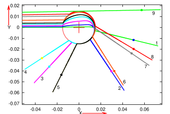
Figure 3: Upper panel: Projections of the rays listed in Table 1 on a surface of constant $t$ along the flow lines of the cosmic dust. Observer I is at $X\approx-0.8898,Y=0$ beyond the left margin of the figure. The large dots mark the intersections of the rays with the last-scattering hypersurface. The dotted circle has the radius $r=A_{1}+B_{1}$, where the BB hump has its edge. More explanation in the text. Lower panel: Ray 9 shown all the way between Observer I and the BB.

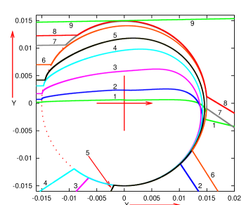
Figure 4: The region near the BB hump in Fig. 3. The arrow on the horizontal arm of the cross points in the direction of the dipole maximum. More explanation in the text.

Ray 0 is not included in the figures because, at their scale, it would coincide with the $Y=0$ axis. It is included in the table in order to show how $1+z_{\rm LSH}$ abruptly jumps from the near-zero value (12) on an axial ray to a large positive value on a ray that is only slightly nonaxial.

The redshifts initially increase with the viewing angle. The maximum $z_{\rm LSH}$ is achieved on Ray 8 inside the image of the source, not at its edge, and it is larger than the background (17). The same thing happened in the L–T/Friedmann model Kras2016a , and will again occur for Observers II and III further in this paper. Ray 9 just grazes the world-tube $r=r_{b}$, and $z_{\rm LSH}$ on it is close to (17). Its $k^{\vartheta}_{o}$ was determined by trial and error: for each ray the program that calculated its path determined the minimum $r\ {\overset{\rm def}{=}}\ r_{cl}$ along it, and Ray 9 is the one where $r_{cl}-r_{b}=0.0000000000735095811$ was reasonably small.

The rays abruptly change their direction every time they come near to the surface $r=r_{b}$. The change is sharper on the second intersection with $r=r_{b}$ where the ray is closer to the BB. When the rays travel over the BB hump further from its edge the deflections are smaller.

The angle of deflection depends on the interval of $t$ that the ray spends near the edge of the BB hump. Ray 1 meets $r=r_{b}$ nearly head-on and does not strongly change direction on first encounter. On second encounter, it is closer to the BB and is forced to bend around more.

The other rays meet the $r=r_{b}$ surface at smaller angles than Ray 1, so they stay near it for longer times. For Rays 3, 4 and 5, this causes a much stronger deflection than for Ray 1. For Rays 6 – 8, another effect prevails: they fly farther from the axis, so they approach the BB at larger $t-t_{B}$ and stay over it for a shorter time; therefore the deflection angle decreases again. Ray 9 does not enter the Szekeres region but only touches it, so it propagates almost undisturbed as in the Friedmann region.

Figures 3 and 4 show only those rays for which $k^{\vartheta}_{o}>0$. The images of the rays with $k^{\vartheta}_{o}<0$ are mirror reflections of those shown. In fact, since $\vartheta=0$ is the axis of symmetry, the image will be the same for every $\varphi$, so one should imagine the complete collection of constant-$\varphi$ null geodesics by rotating Figs. 3 and 4 around the $\vartheta=0$ axis.

IX.2 Rays reaching Observer II

Table 2 and Fig. 5 are analogues of Table 1 and Fig. 4 for Observer II. The analogue of Ray $n$ from Table 1 is Ray $10+n$ in Table 2. The $k^{\vartheta}_{o}$ are the same as in Table 1, with the exception of Ray 19 – see below for an explanation. The angular radii are slightly smaller here because $\Phi_{o}$ for Observer II is slightly smaller than (11):

$$(\Phi_{o})_{\rm obs\ 2}=0.40181424093371831.$$ (19)

But at the level of precision used in the tables, the angular radii for Rays 11 – 18 are the same as those for Rays 1 – 8. The analogue of Ray 0 is not included.

Table 2: Parameters of rays reaching Observer II

Ray	$k^{\vartheta}_{o}$	$1+z$ at LSH
11	0.0005	358.22989174485627
12	0.002	388.80853980783820
13	0.005	408.06476517495747
14	0.009	504.79183448874682
15	0.012	620.08511872418046
16	0.02	885.02972357472424
17	0.03	970.70644144723383
18	0.035	982.13817446295479
19	0.04205	951.83804564661989

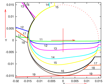
Figure 5: The analogue of Fig. 4 for Observer II, who is at $X\approx 0.889,Y=0$ beyond the right margin of the figure. See Table 2 for the parameters of the rays.

Ray 19 grazes the edge of the Szekeres region – so its $k^{\vartheta}_{0}$ determines the angular radius of the whole source by (16). Since $r_{\rm obs}$ is smaller here, the angular radius for Ray 19 is larger than for Ray 9; it is

$$\alpha_{\rm II}=0.9681^{\circ}.$$ (20)

The values of $1+z_{\rm LSH}$ in Table 2 are different from those in Table 1, but the general pattern is the same: $z_{\rm LSH}$ initially increases with the viewing angle, achieves a maximum inside the image of the source, then decreases to the background value at its edge. The maximum is achieved at the same $k^{\vartheta}_{o}$ as before, on Ray 18.

IX.3 Rays reaching Observer III

Observer III, unlike Observers I and II, is not located on the axis of symmetry, so the (past-directed) rays going off from her position with $k^{\vartheta}_{o}<0$ will not be mirror images of those with $k^{\vartheta}_{o}>0$. Therefore, these two groups of rays are shown in separate tables and separate figures. Table 3 and Fig. 6 contain the rays for which $k^{\vartheta}_{o}\leq 0$; the rays in Table 4 and Fig. 7 have $k^{\vartheta}_{o}>0$. The set of values of $\left|k^{\vartheta}_{o}\right|$ is the same as in Table 1 and Fig. 4. The analogues of Ray $n$ from Table 1 are Ray $20+n$ in Table 3 and Ray $30+n$ in Table 4.

Table 3: Parameters of rays with $k^{\vartheta}_{o}\leq 0$ at Observer III

Ray	$k^{\vartheta}_{o}$	$1+z$ at LSH
20	0.0	342.29964855437106
21	-0.0005	350.64558337051187
22	-0.002	337.49308380652388
23	-0.005	361.19113331483726
24	-0.009	470.62189702521152
25	-0.012	629.72937110236398
26	-0.02	900.56138279350250
27	-0.03	971.41838000807513
28	-0.035	982.30363263812137
29	-0.0425	951.83650139022654

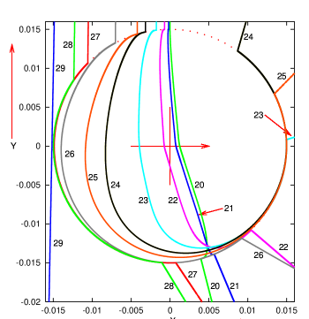
Figure 6: The analogue of Fig. 4 for Observer III, who is at $X=0,Y\approx 0.889$ above the upper edge of the figure. Only the rays with $k^{\vartheta}_{o}\leq 0$ are shown; see Table 3 for their parameters.

The value of $\Phi_{o}$ here is between the previous ones,

$$(\Phi_{o})_{\rm obs\ 3}=0.40192128311507536,$$ (21)

while $t_{o}=0$ does not differ significantly from (20) and (21), so the angular radii would also be intermediate; they are not listed in the tables.

The most conspicuous difference from the previous cases is in Ray 20, which proceeds along $\vartheta=\pi/2$ in the Friedmann region: it is deflected toward larger $\vartheta$ on entry to the Szekeres region, and bends oppositely to all other rays on leaving it. Rays 21 and 22 get deflected so strongly that they cross the line $\vartheta=\pi/2,3\pi/2$ well inside the Szekeres region, unlike their analogues, Rays 1, 2, 11 and 12, which cross the $\vartheta=0,\pi$ lines just before leaving the Szekeres region. Beginning with Ray 23, the paths of the rays become similar (though different in numerical detail) to the corresponding ones for Observers I and II.

The pattern of $1+z_{\rm LSH}$ across the image of the source here is different from those for Observers I and II: with decreasing $k^{\vartheta}_{o}<0$ the redshift achieves a minimum on Ray 22, then a maximum larger than in the background on Ray 28; it then drops to the background value. One ray in this family (not shown) will pass through $r=0$, but with $0\neq\vartheta\neq\pi$, so it will not have $z=-1$ at the BB for the reason indicated under Eq. (4). See also Ref. Kras2016b , where rays passing through $r=0$ were numerically integrated for the same kind of Szekeres dipole (but with a different BB profile and with $a^{2}=0.1$) – only those proceeding along $\vartheta=0,\pi$ had $z\approx-1$ near the BB.

Table 4: Parameters of rays with $k^{\vartheta}_{o}>0$ at Observer III

Ray	$k^{\vartheta}_{o}$	$1+z$ at LSH
31	0.0005	360.79504513233314
32	0.002	381.93470986017479
33	0.005	453.34271919911635
34	0.009	576.90432434248658
35	0.012	682.52857109479601
36	0.02	895.45677016306377
37	0.03	970.72628947084468
38	0.035	982.16761884746518
39	0.0425	951.83650139022654

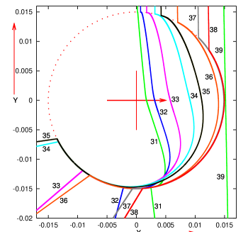
Figure 7: The rays that have $k^{\vartheta}_{o}>0$ at Observer III; see Table 4 for their parameters.

For rays with $k^{\vartheta}_{o}>0$ the pattern of $1+z_{\rm LSH}$ is similar to that for Observer II: there is only the maximum, on Ray 38. However, the values of $1+z_{\rm LSH}$ differ, some of them substantially, from their counterparts in Table 2.

The paths of the rays are similar to those for Observers I and II, but the angle of deflection is smaller for each ray here. Also, the rays bend away from the $X=0$ axis near the $Y=0$ line – this effect was not visible for Observer I and barely noticeable for Observer II.

X Redshift profiles along nonaxial null geodesics

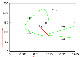
Figure 8: The $z(r)$ relation for Ray 3 from Fig. 3 and its characteristic branches. Observer I is at $r\approx 0.8898$ beyond the right edge of this figure. See text for explanation.

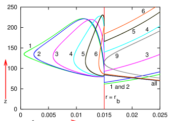
Figure 9: The $z(r)$ relations for Rays 1 – 6 and 9 from Fig. 3. Along Rays 1 – 6, $z$ has two maxima and two minima, which points to the existence of an analogue of the Extremum Redshift Surface along them. Ray 9 does not enter the blueshift-generating region, so $z$ is increasing all along it.

The $z$-profiles along Rays 1 – 6 and 9 are shown in Figs. 8 and 9; they are similar to those in the L–T/Friedmann model Kras2016a . They show that analogues of the ERS (call them ERS’) exist also along nonaxial rays. Figure 8 shows the $z(r)$ relation for Ray 3 in a neighbourhood of $r=r_{b}$; it is a key to reading Fig. 9. In segment (a) of the ray, $z$ increases from 0 at the observer to a local maximum at $r\approx r_{b}$, where the (past-directed) ray intersects the outer branch of the ERS’ for the first time. Then, in segment (b), $z$ decreases to a local minimum at a slightly smaller $r$, where the ray intersects the inner branch of the ERS’ for the first time. Further along the ray, in segment (c), $z$ increases until it reaches the second local maximum at the second intersection of the ray with the inner branch of the ERS’. Then, in segment (d), $z$ decreases up to the second intersection of the ray with the outer branch of the ERS’, where it achieves its second and last local minimum. From then on, in segment (e), $z$ keeps increasing up to $\infty$ achieved at the BB.

Along Rays 1 and 2 in Fig. 9, the second minimum of $z$ is smaller than the first maximum, so those $z(r)$ curves self-intersect.

XI Fitting the radiation sources in the celestial sphere

Imagine a radiation source to be a disk on the celestial sphere of angular radius $\vartheta_{0}$. How many such disks would fit into the celestial sphere at the same time?

An equivalent question is, how many non-overlapping circles of a given radius can be drawn on a sphere of a given radius? A rough answer would be obtained by dividing the surface area of the sphere by the surface area inside the circle. But this would be an overestimate – the circles cannot cover the sphere completely. A better approximation is to inscribe each circle into a quadrangle of arcs of great circles on the sphere. Such figures cannot cover the sphere either, but this method takes into account some of the area outside the circles. Details of the calculation are presented in the Appendix. The area of the sphere divided by the area of the quadrangle is

$${\cal N}=\frac{\pi}{\arcsin\left(\sin^{2}\vartheta_{0}\right)}.$$ (1)

Taking $\vartheta_{0}=0.5^{\circ}$, the current resolution of the GRB detectors (see footnote 2), we obtain

$${\cal N}_{0.5}\approx 41,254.$$ (2)

With $\vartheta_{0}=0.96767^{\circ}$ of Table 1, we obtain

$${\cal N}_{0.96767}\approx 11,014.$$ (3)

Finally, with $\vartheta_{0}=0.9681^{\circ}$, as in (20), we obtain

$${\cal N}_{0.9681}\approx 11,005.$$ (4)

It is instructive to compare these numbers with the number of GRBs detected in observations. This author was not able to get access to a definitive answer, but here is an estimate based on partial information. The BATSE (Burst and Transient Source Explorer) detector, which worked in the years 1991 – 2000, discovered 2704 GRBs BATSE (it was de-orbited in 2000 deorbit ). Assuming the same rate of new discoveries, 8112 GRBs should have been detected between 1991 and now – still fewer than (4).

When the angular radius is divided by $f$, the number of possible sources in the sky should be multiplied by $f^{2}$. Equation (1) approximately confirms this, since for small $\vartheta_{0}$ we have $\sin\vartheta_{0}\approx\vartheta_{0}\approx\arcsin\vartheta_{0}$.)

XII Possible and necessary improvements of the model

The model presented here accounts for the lowest frequency of the radiation in the observed GRBs (the model of highest-frequency GRBs was discussed in Ref. Kras2016a ). The angular radius of the radiation sources seen by the present observer is twice as large as the current observations allow (nearly $1^{\circ}$ in the model vs. $0.5^{\circ}$ – the resolution of the GRB detectors; see footnote 2). In order to decrease this angle, the BB hump that emits the radiation should be made narrower or lower; in the second case it would be further away from the observer seeing the high-frequency flash. The BB profile chosen in this paper cannot be the limit of improvement. The first attempt to explain the GRBs using a cosmological blueshift resulted in a model Krasfail whose hump had the height $A_{0}+B_{0}=0.026$ NTU and width $A_{1}+B_{1}=0.108$. By experimenting with the parameters of the hump, the numbers in (18) were achieved; i.e. the height was decreased $\approx 206$ times and the width 7.2 times. The result of such a blind search cannot be the best possible. In particular, other classes of shapes of the BB hump should be tried.

To get small $1+z$, the BB profile should be such that the blueshifted ray spends as much time as possible traveling above the LSH but below the ERS. As follows from (7) and (8), the room under the ERS becomes larger when ${{\rm d}{t_{B}}}/{{\rm d}{r}}$ is larger and when $a$ is smaller. The problem with small $a$ was described in Sec. VIII, but it might be overcome using a greater numerical precision. A larger ${{\rm d}{t_{B}}}/{{\rm d}{r}}$ tends to make the BB hump higher. In order to keep the hump acceptably low, the large ${{\rm d}{t_{B}}}/{{\rm d}{r}}$ has to be limited to a short interval of $r$ – this is where the steep slope of the hump in Fig. 2 came from.

A serious limitation is the fact mentioned in Sec. VII that the ERS is tangent to the BB at $r=0$. If this could be overcome, the rays would stay in the blueshift-generating region (below the ERS) for a longer time interval, and so the required $1+z$ range could be achieved with a lower or narrower hump.

Further optimizations are possible. For example, the function $E(r)$ here has the Friedmann shape (12) throughout the Szekeres region – obviously one should check what happens when it has other shapes. Friedmann backgrounds other than the one of Sec. IV should be tested. Szekeres dipoles other than (19) should also be tested, in particular non-axially-symmetric ones. Carrying out such tests is laborious – it involves finding, by numerical shooting, the minimum of a function of several variables (in this paper these were 7 variables: the five in (18), the $a$ of (19) and the $\Delta t_{c}$ of (4)).

Similar to the L–T model of Ref. Kras2016a , the model presented here implies too-long durations for the high-frequency flashes and for their afterglows. This is because, in axially symmetric models, once the observer and the source are placed on the symmetry axis, they stay there forever – the source does not drift KrBo2011 ; QABC2012 ; KoKo2017 . The only changes of the observed frequency and intensity may then occur because the observer receives rays emitted from different points of the BB hump along the same line of sight, so the changes occur on the cosmological time scale and are much slower than in the observed GRBs (see Ref. Kras2016a for the numbers).

A nonsymmetric Szekeres model offers a new possibility. In such a model there also exist two opposite directions along which radiation is strongly blueshifted Kras2016b . However, the cosmic drift KrBo2011 ; QABC2012 ; KoKo2017 will cause an observer who was initially in the path of one of those preferred rays to be off it after a while. The time scale of this process should be short, as a consequence of the very large distance between the source and the observer and of the discontinuous change from blueshift to redshift as soon as the strongly blueshifted ray misses the observer.

One solution of the duration problem has already been tested, and will be submitted for publication soon. If there is another QSS region between the radiation source and the observer, then the cosmic drift in the intervening QSS region will cause the highest-frequency ray to miss the observer after 10 minutes or less. This satisfactorily solves the problem of the duration of the high-frequency flash, but not the problem of the duration of the afterglow. The latter still awaits solution.

XIII Summary and conclusions

In Ref. Kras2016b , existence and properties of blueshifts in exemplary simple quasispherical Szekeres models were investigated. Using that knowledge, in the present paper it was investigated whether a QSS mass dipole superposed on a L–T background would allow better mimicking of gamma-ray bursts by cosmological blueshifting than in Ref. Kras2016a , where pure L–T models were used.

The axially symmetric QSS model was introduced in Secs. II and III. The QSS region is matched to a negative-spatial-curvature Friedmann background (Sec. IV), chosen for correspondence with earlier papers by this author Kras2014d ; Kras2014a . After presenting definitions and preliminary information in Secs. V, VI and VII, in Sec. VIII the parameters of the QSS model are chosen such that at present the highest frequency of the blueshifted radiation agrees with the lowest frequency of the observed GRBs (this agreement requires that the blueshift between the last scattering and the present time obeys $1+z\leq 1.689\times 10^{-5}$ Kras2016a ). The introduction of the Szekeres dipole has the consequence that the required $1+z$ is achieved with a lower hump in the BB profile, which is thus at a greater distance from the observer than in the L–T model. In Sec. IX, the paths of nonaxial light rays reaching three different present observers are presented. The observers are placed in prolongation of the mass-dipole maximum axis, of the dipole minimum axis, and of the dipole equator. The distributions of the observed redshift across the image of the source are different for each observer, and the angular radii of the source are between $0.96767^{\circ}$ and $0.9681^{\circ}$. This is nearly twice as much as the current GRB observations allow, but the model has the potential to be improved (see Sec. XII). In Sec. X, the redshift profiles along nonaxial rays were calculated in order to show that extrema of redshift also exist along them. In Sec. XI it was estimated that with the angular radii of the radiation sources being between $0.96767^{\circ}$ and $0.9681^{\circ}$, approximately 11,000 such sources could be simultaneously fitted into the sky of the present observer. Finally, possible further improvements in the model were discussed in Sec. XII.

The models of generating the high-frequency radiation flashes discussed here and in Ref. Kras2016a are subject to two kinds of tests:

1. In the future, the observers should be able to resolve the fuzzy disks they now see as GRB sources (see footnote 2), and measure the distribution of radiation frequencies and intensities across them. Then it will be possible to compare those distributions with model predictions. A model that would predict such a distribution correctly could then be used to get information about the sources.

2. If the gamma flashes are generated simultaneously with the CMB radiation, as proposed here and in Ref. Kras2016a , then they are observed now as short-lived because its source comes into and out of the observer’s view, but has existed there since the last-scattering epoch. In this case, the central high-frequency ray should be surrounded by rays with positive redshifts smoothly blending with the CMB background at the edge of the source image, as shown in tables in Sec. IX. But if a source of the radiation flash lies later than the last scattering, then it is independent of the CMB. It should black out all CMB rays within some angle around the central ray, and the redshift profile across the image of the source would not need to continuously match the CMB at the edge.

This author does not wish to question the validity of the GRB models proposed so far. The motivation for this work was this: history of science teaches us that if a well-tested theory predicts a phenomenon, then the prediction has to be taken seriously and checked against experiments and observations. Since general relativity clearly predicts that some of the light generated during last scattering might reach us with strong blueshift, consequences of this prediction have to be worked out and submitted to tests. In trying to accommodate blueshifts, the suspicion fell on the GRBs because it is generally agreed that at least some of their sources lie billions of years to the past from now Perlwww . The BB humps discussed here would lie about twice as far, at $\approx 13.6$ Gyr to the past, by (16). For the relativity theory, it would be interesting to know whether at least some of the observed GRBs are powered by the mechanism discussed here.

Appendix A How many circles of a given radius can be drawn on a sphere of a given radius?

Imagine a circle K drawn on a sphere S of radius $a$ and a cone that intersects S along K and has its vertex at the center of S; see Figs. 10 and 11. Let the opening angle of the cone be $\vartheta_{0}$. Now imagine a square pyramid circumscribed on this cone. The pyramid intersects S along the curvilinear quadrangle shown in thicker lines in Fig. 10. The part of S inside the quadrangle has the surface area 8 times the surface area inside the curvilinear triangle ABC; see also Fig. 12.

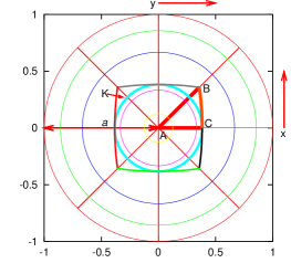
Figure 10: View from the $z>0$ axis on the cone and the pyramid. They intersect the sphere along the circle K and the curvilinear quadrangle shown in thicker lines, respectively.

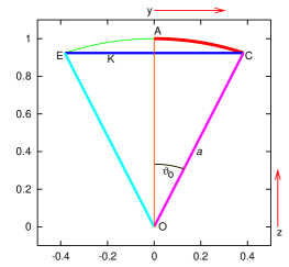
Figure 11: Projection of the cone and of the pyramid from Fig. 10 on the $x=0$ coordinate plane. The lines OE and OC are intersections of the cone (and of the faces of the pyramid) with the plane of the figure; the letters K, A and C have the same meaning as in Fig. 10.

Figure 12: A sketch to calculate the surface area of the triangle ABC on a sphere. See text.

Suppose the center of the sphere is at $x=y=z=0$, so the equation of the sphere is $x^{2}+y^{2}+z^{2}=a^{2}$, and the axis of the cone goes along the $z$ axis. The metric of the sphere in the $(x,y)$ coordinates is

$${\rm d}x^{2}+{\rm d}y^{2}+{\rm d}z^{2}=$$ (1)

$$\frac{\left(a^{2}-y^{2}\right){\rm d}x^{2}+2xy{\rm d}x{\rm d}y+\left(a^{2}-x^{2}\right){\rm d}y^{2}}{a^{2}-x^{2}-y^{2}},$$

and so the surface element of the sphere is

$$\sqrt{g}{\rm d}x{\rm d}y=\frac{a}{\sqrt{a^{2}-x^{2}-y^{2}}}{\rm d}x{\rm d}y.$$ (2)

The side AC of the triangle lies in the plane $x=0$, and $y$ on it changes from 0 to $a\sin\vartheta_{0}$. The side AB lies in the plane $y=x$. The $y$-coordinate of the point B is

$$y_{\rm B}=\frac{a\sin\vartheta_{0}}{\sqrt{1+\sin^{2}\vartheta_{0}}},$$ (3)

as is easy to calculate knowing that this point lies simultaneously on the sphere $x^{2}+y^{2}+z^{2}=a^{2}$, in the plane $y=x$ and in the plane $z=y\cot\vartheta_{0}$ that contains the right face of the pyramid. The auxiliary point D has the same $y$-coordinate as B. The arc BC (which is part of the intersection of the right face of the pyramid with the sphere) obeys the equation

$$x=\sqrt{a^{2}-\frac{y^{2}}{\sin^{2}\vartheta_{0}}}\ {\overset{\rm def}{=}}\ x_{\rm BC}(y).$$ (4)

The surface area of the triangle ABC is thus

$$S_{\rm ABC}=\int_{0}^{y_{\rm B}}{\rm d}y\int_{0}^{y}\frac{a}{\sqrt{a^{2}-x^{2}-y^{2}}}\ {\rm d}x$$

$$+\int_{y_{\rm B}}^{a\sin\vartheta_{0}}{\rm d}y\int_{0}^{x_{\rm BC}(y)}\frac{a}{\sqrt{a^{2}-x^{2}-y^{2}}}\ {\rm d}x$$ (5)

$$=\int_{0}^{y_{\rm B}}a\arcsin\left(\frac{y}{\sqrt{a^{2}-y^{2}}}\right){\rm d}y$$

$$+\int_{y_{\rm B}}^{a\sin\vartheta_{0}}a\arcsin\left(\frac{x_{\rm BC}(y)}{\sqrt{a^{2}-y^{2}}}\right){\rm d}y.$$ (6)

The two integrals in (6) are

$$S_{I} = \frac{a^{2}\vartheta_{0}\sin\vartheta_{0}}{\sqrt{1+\sin^{2}\vartheta_{0}}}-\tfrac{1}{2}\ a^{2}\arcsin\left(\sin^{2}\vartheta_{0}\right),$$ (7)

$$S_{II} = -\frac{a^{2}\vartheta_{0}\sin\vartheta_{0}}{\sqrt{1+\sin^{2}\vartheta_{0}}}+a^{2}\arcsin\left(\sin^{2}\vartheta_{0}\right).$$ (8)

So, the area of the triangle ABC is $\tfrac{1}{2}\ a^{2}\arcsin\left(\sin^{2}\vartheta_{0}\right)$, and the area of the quadrangle in Fig. 10 is

$$S_{\rm quad}=4a^{2}\arcsin\left(\sin^{2}\vartheta_{0}\right).$$ (9)

(When $\vartheta_{0}=\pi/2$, this gives the obvious result $2\pi a^{2}$.)

Hints for the less-trivial parts of calculating the integrals:

In $S_{I}$ change the variables by $\arcsin\left(\frac{y}{\sqrt{a^{2}-y^{2}}}\right)=w$ and integrate by parts to get rid of the factor $w$ under the integral.

In $S_{II}$ change the variables by $y=a\sin\vartheta_{0}\sin u$, then integrate by parts to get rid of $\arcsin$ under the integral, and finally use the identity $\arctan\lambda=\arcsin\left(\frac{\lambda}{\sqrt{1+\lambda^{2}}}\right)$.

Now an approximate answer to the question in the title can be given. The quadrangles will not cover the whole surface of the sphere, but by dividing the surface area of the sphere, $4\pi a^{2}$, by $S_{\rm quad}$, we obtain an upper bound on the number of nonoverlapping circles that can be drawn on the sphere; it is (1).