Maximal violation of Bell inequalities under local filtering

Abstract

We investigate the behavior of the maximal violations of the CHSH inequality and V$\grave{e}$rtesi’s inequality under the local filtering operations. An analytical method has been presented for general two-qubit systems to compute the maximal violation of the CHSH inequality and the lower bound of the maximal violation of V$\acute{e}$rtesi’s inequality over the local filtering operations. We show by examples that there exist quantum states whose non-locality can be revealed after local filtering operation by the V$\acute{e}$rtesi’s inequality instead of the CHSH inequality.

^∗ Correspondence to liming@upc.edu.cn

Quantum mechanics is inherently nonlocal. After performing local measurements on a composite quantum system, non-locality, which is incompatible with local hidden variable theory [1] can be revealed by Bell inequalities. The non-locality is of great importance both in understanding the conceptual foundations of quantum theory and in investigating quantum entanglement. It is also closely related to certain tasks in quantum information processing, such as building quantum protocols to decrease communication complexity [2, 3] and providing secure quantum communication [4, 5]. We refer to [6] for more details.

To determine whether a quantum state has non-locality, it is sufficient to construct a Bell inequality[7, 8, 9, 10, 11, 12, 13] which can be violated by the quantum state. For two qubits systems, Clauser-Horne-Shimony-Holt have presented the famous CHSH inequality [7].

Let ${\mathcal{B}_{CHSH}}$ denote the Bell operator for the CHSH inequality,

$${\mathcal{B}_{CHSH}}=A_{1}\otimes B_{1}+A_{1}\otimes B_{2}+A_{2}\otimes B_{1}-A_{2}\otimes B_{2},$$ (1)

with $A_{i}$ and $B_{j}$ being the observables of the form $A_{i}=\sum_{k=1}^{3}a_{ik}\sigma_{k}$ and $B_{j}=\sum_{l=1}^{3}b_{jl}\sigma_{l}$ respectively, $i,j=1,2$,

$$\sigma_{1}=\left(\begin{array}[]{cc}-1&0\\ 0&1\\ \end{array}\right),~{}~{}\sigma_{2}=\left(\begin{array}[]{cc}0&1\\ 1&0\\ \end{array}\right)\mbox{ and }\sigma_{3}=\left(\begin{array}[]{cc}0&i\\ -i&0\\ \end{array}\right)$$ (2)

are the Pauli matrices. For any two-qubit quantum state $\rho$, the maximal violation of the CHSH inequality (MVCI) is given by [14]

$$\max_{\mathcal{B_{CHSH}}}|\langle{\mathcal{B_{CHSH}}}\rangle_{\rho}|=2\sqrt{\tau_{1}+\tau_{2}},$$ (3)

where $\tau_{1}$ and $\tau_{2}$ are the two largest eigenvalues of the matrix $T^{{\dagger}}T$, $T$ is the matrix with entries $T_{\alpha\beta}=tr[\rho\,\sigma_{\alpha}\otimes\sigma_{\beta}]$, $\alpha,\,\beta=1,2,3$. For a state admitting local hidden variable (LHV) model, one has $\max_{\mathcal{B_{CHSH}}}|\langle{\mathcal{B_{CHSH}}}\rangle_{LHV}|\leq 2$.

Another effective Bell inequality for two-qubit system is given by the Bell operator [15] V$\acute{e}$rtesi

$$\mathcal{B_{V}}=\frac{1}{n^{2}}[\sum_{i,j=1}^{n}A_{i}\otimes B_{j}+\sum_{1\leq i<j\leq n}C_{ij}\otimes(B_{i}-B_{j})+\sum_{1\leq i<j\leq n}(A_{i}-A_{j})\otimes D_{ij}],$$ (4)

where $A_{i},B_{j},C_{ij}$ and $D_{ij}$ are observables of the form $\sum_{\alpha=1}^{3}x_{\alpha}\sigma_{\alpha}$ with $\vec{x}=(x_{1},x_{2},x_{3})$ the unit vectors.

The maximal violation of V$\acute{e}$rtesi’s inequality(MVVI) is lower bounded by the following inequality [20]. For arbitrary two-qubit quantum state $\rho$, we have

$$\max_{\mathcal{B_{V}}}|\langle{\mathcal{B_{V}}}\rangle_{\rho}| \geq \max_{a,b,c,d}\left[\frac{1}{s_{ab}s_{cd}}|\int_{\Omega_{a}^{b}\times\Omega_{c}^{d}}<\vec{x},T\vec{y}>d\mu(\vec{x})d\mu(\vec{y})|+\frac{1}{2s^{2}_{cd}}\int_{\Omega_{c}^{d}\times\Omega_{c}^{d}}|T(\vec{x}-\vec{y})|d\mu(\vec{x})d\mu(\vec{y})\right.$$ (5)

$$\left.+\frac{1}{2s^{2}_{ab}}\int_{\Omega_{a}^{b}\times\Omega_{a}^{b}}|T^{{\dagger}}(\vec{x}-\vec{y})|d\mu(\vec{x})d\mu(\vec{y})\right],$$

where $s_{\alpha\beta}=\int_{\Omega_{\alpha}^{\beta}}d\mu(\vec{x})$. The maximum on the right side of the inequality goes over all the integral area $\Omega_{a}^{b}\times\Omega_{c}^{d}$ with $0\leq a<b\leq\frac{\pi}{2}$ and $0\leq c<d\leq\frac{\pi}{2}$. Here the maximal value $\max_{\mathcal{B_{V}}}|\langle{\mathcal{B_{V}}}\rangle_{\rho}|$ of a state $\rho$ admitting LHV model is upper bounded by $1$.

The maximal violation of a Bell inequality above is derived by optimizing the observables for a given quantum state. With the formulas (3) and (5) one can directly check if a two-qubit quantum state violates the CHSH or the V$\acute{e}$rtesi’s inequality. It has been shown that the maximal violation of a Bell inequality is in a close relation with the fidelity of the quantum teleportation [17] and the device-independent security of quantum cryptography [18].

The maximal violation of a Bell inequality can be enhanced by local filtering operations [21]. In [22], the authors present a class of two-qubit entangled states admitting local hidden variable models, and show that the states after local filtering violate a Bell inequality. Hence, there exist entangled states, the non-locality of which can be revealed by using a sequence of measurements.

In this manuscript, we investigate the behavior of the maximal violations of the CHSH inequality and V$\acute{e}$rtesi’s inequality under local filtering operations. An analytical method has been presented for any two-qubit system to compute the maximal violation of the CHSH inequality and the lower bound of the maximal violation of V$\acute{e}$rtesi’s inequality under local filtering operations. The corresponding optimal local filtering operation is derived. We show by examples that there exist quantum states whose nonlocality can be revealed after local filtering operation by V$\acute{e}$rtesi’s inequality instead of the CHSH inequality.

Results

We consider the CHSH inequality for two-qubit systems first. Before the Bell test, we apply the local filtering operation on a state $\rho\in{\cal{H}}={\cal{H}}_{A}\otimes{\cal{H}}_{B}$ with $dim\,{\cal{H}}_{A}=dim\,{\cal{H}}_{B}=2$. $\rho$ is mapped to the following form under local filtering transformations [19, 22]:

$$\rho^{\prime}=\frac{1}{N}(F_{A}\otimes F_{B})\rho(F_{A}\otimes F_{B})^{{\dagger}},$$ (6)

where $N=tr[(F_{A}\otimes F_{B})\rho(F_{A}\otimes F_{B})^{{\dagger}}]$ is a normalization factor, and $F_{A/B}$ are positive operators acting on the subsystems respectively. Such operations can be a local interaction with the dichroic environments[23].

For two-qubit systems, let $F_{A}=U\Sigma_{A}U^{{\dagger}}$ and $F_{B}=V\Sigma_{B}V^{{\dagger}}$ be the spectral decompositions of $F_{A}$ and $F_{B}$ respectively, where $U$ and $V$ are unitary operators. Define that

$$\delta_{k}=\Sigma_{A}\sigma_{k}\Sigma_{A},~{}~{}~{}\eta_{l}=\Sigma_{B}\sigma_{l}\Sigma_{B}$$ (7)

and $X$ be a matrix with entries given by

$$x_{kl}=tr[\varrho\delta_{k}\otimes\eta_{l}],~{}~{}~{}k,l=1,2,3,$$ (8)

where $\varrho$ is locally unitary with $\rho$.

we have the following theorem.

Theorem 1: The maximal quantum bound of a two-qubit quantum state $\rho^{\prime}=\frac{1}{N}(F_{A}\otimes F_{B})\rho(F_{A}\otimes F_{B})^{{\dagger}}$ is given by

$$\max_{\mathcal{B_{CHSH}}}|\langle{\mathcal{B_{CHSH}}}\rangle_{\rho^{\prime}}|=\max_{\varrho}2\sqrt{\tau^{\prime}_{1}+\tau^{\prime}_{2}},$$ (9)

where $\tau^{\prime}_{1}$ and $\tau^{\prime}_{2}$ are the two largest eigenvalues of the matrix $X^{{\dagger}}X/N^{2}$ with $X$ given by (8). The left max is taken over all $B_{CHSH}$ operators, while the right max is taken over all $\varrho$ that are locally unitary equivalent to $\rho$.

See Methods for the proof of theorem 1.

Now we investigate the behavior of the V$\grave{e}$rtesi-Bell inequality under local filtering operations. In [20] we have found an effective lower bound for the MVVI by considering infinite many measurements settings, $n\to\infty$. Then the discrete summation in (4) is transformed into an integral of the spherical coordinates over the sphere $S^{2}\subset{R^{3}}$. We denote the spherical coordinate of $S^{2}$ by $(\phi_{1},\phi_{2})$. A unit vector $\vec{x}=(x_{1},x_{2},x_{3})$ can be parameterized by $x_{1}=\sin{\phi_{1}}\sin{\phi_{2}}$, $x_{2}=\sin{\phi_{1}}\cos\phi_{2}$, $x_{3}=\cos{\phi_{1}}$. For any $0\leq a\leq b\leq\frac{\pi}{2},$ we denote $\Omega_{a}^{b}=\{x\in S^{2}:a\leq\phi_{1}(x)\leq b\}.$

Theorem 2: For two-qubit quantum state $\rho^{\prime}$ given by (6), we have

$$\max_{\mathcal{B_{V}}}|\langle\mathcal{B_{V}}\rangle_{\rho^{\prime}}| \geq\max_{a,b,c,d}\frac{1}{N}\left[\frac{1}{s_{ab}s_{cd}}|\int_{\Omega_{a}^{b}\times\Omega_{c}^{d}}<\vec{x},X\vec{y}>d\mu(\vec{x})d\mu(\vec{y})|\right.$$

$$+\frac{1}{2s^{2}_{cd}} \left.\int_{\Omega_{c}^{d}\times\Omega_{c}^{d}}|X(\vec{x}-\vec{y})|d\mu(\vec{x})d\mu(\vec{y})+\frac{1}{2s^{2}_{ab}}\int_{\Omega_{a}^{b}\times\Omega_{a}^{b}}|X^{t}(\vec{x}-\vec{y})|d\mu(\vec{x})d\mu(\vec{y})\right],$$ (10)

where $X$ is defined by (8). $X^{t}$ stands for the transposition of $X$, and $s_{\alpha\beta}=\int_{\Omega_{\alpha}^{\beta}}d\mu(\vec{x})$. The maximization on the right side of the inequality goes over all the integral area $\Omega_{a}^{b}\times\Omega_{c}^{d}$ with $0\leq a<b\leq\frac{\pi}{2}$ and $0\leq c<d\leq\frac{\pi}{2}$.

See Methods for the proof of theorem 2.

Remark: The right hand sides of (9) and (Maximal violation of Bell inequalities under local filtering) depend just on the state $\sigma$ which is local unitary equivalent to $\rho$. Thus to compare the difference of the maximal violation for $\rho$ and that for $\rho^{\prime}$, it is sufficient to just consider the difference between $\sigma$ and $\rho^{\prime}$.

Without loss of generality, we set

$$\Sigma_{A}=\left(\begin{array}[]{cc}x&0\\ 0&1\\ \end{array}\right)~{}\mbox{ and }~{}~{}\Sigma_{B}=\left(\begin{array}[]{cc}y&0\\ 0&1\\ \end{array}\right)$$ (11)

with $x,y\geq 0$. According to the definition of $\delta_{k}$ and $\eta_{l}$ in (7), one computes that

$$\delta_{1}=\left(\begin{array}[]{cc}-x^{2}&0\\ 0&1\\ \end{array}\right),\ \ \ \ \delta_{2}=\left(\begin{array}[]{cc}0&x\\ x&0\\ \end{array}\right)\mbox{ and }\delta_{3}=\left(\begin{array}[]{cc}0&ix\\ -ix&0\\ \end{array}\right);$$ (12)

$$\eta_{1}=\left(\begin{array}[]{cc}-y^{2}&0\\ 0&1\\ \end{array}\right),\ \ \ \ \eta_{2}=\left(\begin{array}[]{cc}0&y\\ y&0\\ \end{array}\right)\mbox{ and }\eta_{3}=\left(\begin{array}[]{cc}0&iy\\ -iy&0\\ \end{array}\right).$$ (13)

Let $\sigma_{0}=\left(\begin{array}[]{cc}1&0\\ 0&1\\ \end{array}\right).$ Set $\vec{\delta}=(\delta_{1},\delta_{2},\delta_{3})$, $\vec{\eta}=(\eta_{1},\eta_{2},\eta_{3})$, and $\vec{\sigma}=(\sigma_{0},\sigma_{1},\sigma_{2},\sigma_{3})$. We have $\vec{\delta}=C\vec{\sigma}$ and $\vec{\eta}=D\vec{\sigma}$, where

$$C=\left(\begin{array}[]{cccc}\frac{1}{2}(1-x^{2})&\frac{1}{2}(1+x^{2})&0&0\\ 0&0&x&0\\ 0&0&0&x\\ \end{array}\right){\rm and}\quad D=\left(\begin{array}[]{cccc}\frac{1}{2}(1-y^{2})&\frac{1}{2}(1+y^{2})&0&0\\ 0&0&y&0\\ 0&0&0&y\\ \end{array}\right){\rm respectively}.$$ (14)

Then one has $x_{kl}=(CWD^{{\dagger}}),$ where $W$ is a $4\times 4$ matrix with entries $w_{\alpha\beta}=tr[\sigma\sigma_{\alpha}\otimes\sigma_{\beta}]$. Let $\tilde{O}_{A}=\left(\begin{array}[]{cc}1&0\\ 0&O_{A}\\ \end{array}\right)$ and $\tilde{O}_{B}=\left(\begin{array}[]{cc}1&0\\ 0&O_{B}\\ \end{array}\right)$ where $O_{A}$ and $O_{B}$ are $3\times 3$ orthogonal operators. Define that $\vec{r}$ and $\vec{s}$ be three dimensional vectors with entries $r_{i}=tr[\rho\sigma_{0}\otimes\sigma_{i}]$ and $s_{j}=tr[\rho\sigma_{j}\otimes\sigma_{0}]$ respectively. And let $\tilde{T}=\left(\begin{array}[]{cc}1&\vec{r}\\ \vec{s}&T\\ \end{array}\right).$ One can further show that

$$X=CWD^{{\dagger}}=C\tilde{O}_{A}\tilde{T}\tilde{O}_{B}^{{\dagger}}D^{{\dagger}},$$ (15)

and

$$N=x_{+}y_{+}+4x_{-}y_{+}(O_{A}\vec{s})_{1}+4x_{+}y_{-}(O_{B}\vec{r})_{1}+4x_{-}y_{-}(O_{A}TO_{B}^{t})_{11},$$ (16)

where $x_{+}=\frac{1}{2}(1+x^{2})$, $x_{-}=\frac{1}{2}(1-x^{2})$, $y_{+}=\frac{1}{2}(1+y^{2})$ and $y_{-}=\frac{1}{2}(1-y^{2})$. Numerically, one can parameterize $O_{A}$ and $O_{B}$ and then search for the maximization in theorem 1. For the lower bound in theorem 2, we refer to [20].

Corollary: For two-qubit Werner state[27] $\rho_{w}=p|\psi^{-}\rangle\langle\psi^{-}|+(1-p)\frac{I}{4}$, with $|\psi^{-}\rangle=(|01\rangle-|10\rangle)/\sqrt{2}$, one computes $T=\left(\begin{array}[]{ccc}-p&0&0\\ 0&-p&0\\ 0&0&-p\\ \end{array}\right).$ Then by using the symmetric property of the state, (15) and (16), together with theorem 1, we have

$$\max_{\mathcal{B_{CHSH}}}|\langle{\mathcal{B_{CHSH}}}\rangle_{\rho^{\prime}}|=2\sqrt{\tau^{\prime}_{1}+\tau^{\prime}_{2}},$$ (17)

where $\tau^{\prime}_{1}$ and $\tau^{\prime}_{2}$ are the two largest eigenvalues of the matrix $X^{{\dagger}}X/N^{2}$ with $X$ given by

$$x_{kl}=tr[\rho_{w}\delta_{k}\otimes\eta_{l}],~{}~{}~{}k,l=1,2,3.$$ (18)

Applications

In the following we discuss the applications of local filtering. First we show that a state which does not violate the CHSH and the V$\acute{e}$rtesi’s inequalities could violate these inequalities after local filtering. Consider the following density matrix for two-qubit systems:

$$\varrho_{1}=\frac{1}{4}(I\otimes I+r\sigma_{1}\otimes I-p\sum_{i}^{3}\sigma_{i}\otimes\sigma_{i}),$$ (19)

where $-0.3104\leq p\leq 0.7$ to ensure the positivity of $\varrho_{1}$. By using the positive partial transposition criteria one has that $\varrho_{1}$ is separable for $-0.3104\leq p\leq 0.3104$.

Case 1: Set $r=0.3$. It is direct to verify that both the CHSH inequality and V$\acute{e}$rtesi’s inequalities fail to detect the non-locality for the whole region $-0.3104\leq p\leq 0.7$. After filtering, non-locality can be detected for $0.6291\leq p\leq 0.7$ (by Theorem 2) and $0.6164\leq p\leq 0.7$ (by Theorem 1) respectively, see Fig.1.

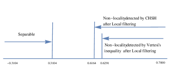
Figure 1: For $r=0.3$, both the CHSH inequality and Vértesi’s inequality fail to detect the non-locality of $\varrho_{1}$ for the whole parameter region of $p$. After local filtering, non-locality is detected for $0.6291\leq p\leq 0.7$ (by Theorem 2) and $0.6164\leq p\leq 0.7$ (by Theorem 1) respectively.

Case 2: Set $p=0.7050$ and $r=0.0400$. The MVCI of $\varrho_{1}$ is $1.994$ without local filtering and $1.9988$ after local filtering, which means that the CHSH inequality is always satisfied before and after local filtering. The lower bound (5) for $\varrho_{1}$ is computed to be less than one, implying the non-locality can not be detected by the lower bound for MVVI derived in [20] without local filtering. However, by taking $x=y=1.1,a=c=0.1671,b=d=1.1096$, from Theorem 2 we have the maximal violation value $1.0005$ which is larger than one. Therefore, after local filtering the state’s non-locality is detected.

Next we give an example that a state admits local hidden variable model (LHV) can violate the Bell inequality under local filtering. Consider two-qubit quantum states with density matrices of the following form:

$$\varrho_{2}=\frac{1}{4}(I\otimes I+p\sigma_{1}\otimes I+p\sum_{i}^{3}\sigma_{i}\otimes\sigma_{i}).$$ (20)

According to the positivity of a density matrix, we have $-0.5\leq p\leq 0.3090$. By using the positive partial transposition criteria [24], one checks that $\varrho_{2}$ is entangled for $-0.5\leq p\leq-0.3090$. The quantum state satisfies the CHSH inequality for the whole parameter region.

We first show that the state $\varrho_{2}$ admits LHV models for $-0.5\leq p\leq-0.3090$.

First we rewrite $\varrho_{2}$ as a convex combination of singlet and separable states,

$$\varrho_{2}=q|\psi_{-}\rangle\langle\psi_{-}|+(1-q)[\frac{1}{2}(I-\frac{q}{1-q}\sigma_{1})\otimes\frac{I}{2}],$$ (21)

where $|\psi_{-}\rangle\langle\psi_{-}|=\frac{1}{4}(I\otimes I-\sum^{3}_{i=1}\sigma_{i}\otimes\sigma_{i})$ and $q=-p$. According to [16], with a visibility of $q=\frac{1}{2}$, the correlations of measurement outcomes produced by measuring the observables $A=\overrightarrow{a}\cdot\overrightarrow{\sigma}$ and $B=\overrightarrow{b}\cdot\overrightarrow{\sigma}$ on the singlet state can be simulated by an LHV model in which the hidden variable $\overrightarrow{\lambda}_{s}\in\mathbf{S}^{2}$ is biased distributed with probability density

$$\rho(\overrightarrow{\lambda}_{s}|\overrightarrow{a})=\frac{|\overrightarrow{a}\cdot\overrightarrow{\lambda}_{s}|}{2\pi}.$$ (22)

With probability $0<q\leq\frac{1}{2}$, Alice and Bob can share the biased distributed variable resource and output $a=-sgn(\overrightarrow{a}\cdot\overrightarrow{\lambda}_{s})$ and $b=sgn(\overrightarrow{b}\cdot\overrightarrow{\lambda}_{s})$, respectively. With probability $1-q$, Alice outputs $a=\pm 1$ with probability $p(a|\overrightarrow{a})=tr[\frac{1}{2}(I-\frac{q}{1-q}\sigma_{z})\frac{I\pm\overrightarrow{a}\cdot\overrightarrow{\lambda}_{s}}{2}]$, and Bob outputs $\pm 1$ with probability $p(b|\overrightarrow{b})=\frac{1}{2}$. Then we can simulate the correlations produced by measuring obesrvables $A$ and $B$ on $\varrho_{2}$,

$$p(a,b|\overrightarrow{a},\overrightarrow{b},\varrho_{2})=tr(\frac{I+a\overrightarrow{a}\overrightarrow{\sigma}}{2}\otimes\frac{I+b\overrightarrow{b}\overrightarrow{\sigma}}{2}\rho)=\frac{1-qab\overrightarrow{a}\cdot\overrightarrow{b}}{4}-\frac{aa_{3}q}{4},$$ (23)

which can be given by the following LHV model,

$$p(a,b|\overrightarrow{a},\overrightarrow{b},\varrho_{2})= q\int_{\mathbf{S}^{2}}p(a|\overrightarrow{a},\overrightarrow{\lambda}_{s})p(b|\overrightarrow{b}\cdot\overrightarrow{\lambda}_{s})\rho(\overrightarrow{\lambda}_{s})d\overrightarrow{\lambda}_{s}+(1-q)p(a\rvert\overrightarrow{a})p(b\rvert\overrightarrow{b})$$ (24)

$$= q\int_{\Omega_{a,b}}\frac{|\overrightarrow{a}\cdot\overrightarrow{\lambda}_{s}|}{2\pi}d\overrightarrow{\lambda}_{s}+(1-q)p(a|\overrightarrow{a})p(b|\overrightarrow{b}),$$

where $\Omega_{a,b}=\{\overrightarrow{\lambda}_{s}|-sgn(\overrightarrow{a}\cdot\overrightarrow{\lambda}_{s})=a\}\cap\{\overrightarrow{\lambda}_{s}|b=sgn(\overrightarrow{b}\cdot\overrightarrow{\lambda}_{s})\}$. Explicitly,

$$p(1,1\arrowvert\overrightarrow{a},\overrightarrow{b},\overrightarrow{\lambda}_{s})=q\int_{\Omega_{1,1}}\frac{|\overrightarrow{a}\cdot\overrightarrow{\lambda}_{s}|}{2\pi}d\overrightarrow{\lambda}_{s}+\frac{1-q}{2}tr[\frac{1}{2}(I-\frac{q}{1-q}\sigma_{z})\frac{I+\overrightarrow{a}\cdot\overrightarrow{\lambda}_{s}}{2}],$$

$$p(1,-1\arrowvert\overrightarrow{a},\overrightarrow{b},\overrightarrow{\lambda}_{s})=q\int_{\Omega_{1,-1}}\frac{|\overrightarrow{a}\cdot\overrightarrow{\lambda}_{s}|}{2\pi}d\overrightarrow{\lambda}_{s}+\frac{1-q}{2}tr[\frac{1}{2}(I-\frac{q}{1-q}\sigma_{z})\frac{I+\overrightarrow{a}\cdot\overrightarrow{\lambda}_{s}}{2}],$$

$$p(-1,1\arrowvert\overrightarrow{a},\overrightarrow{b},\overrightarrow{\lambda}_{s})=q\int_{\Omega_{-1,1}}\frac{|\overrightarrow{a}\cdot\overrightarrow{\lambda}_{s}|}{2\pi}d\overrightarrow{\lambda}_{s}+\frac{1-q}{2}tr[\frac{1}{2}(I-\frac{q}{1-q}\sigma_{z})\frac{I-\overrightarrow{a}\cdot\overrightarrow{\lambda}_{s}}{2}],$$

$$p(-1,-1\arrowvert\overrightarrow{a},\overrightarrow{b},\overrightarrow{\lambda}_{s})=q\int_{\Omega_{-1,-1}}\frac{|\overrightarrow{a}\cdot\overrightarrow{\lambda}_{s}|}{2\pi}d\overrightarrow{\lambda}_{s}+\frac{1-q}{2}tr[\frac{1}{2}(I-\frac{q}{1-q}\sigma_{z})\frac{I-\overrightarrow{a}\cdot\overrightarrow{\lambda}_{s}}{2}],$$

where $\Omega_{1,1}=\{\overrightarrow{\lambda}_{s}\arrowvert\overrightarrow{a}\cdot\overrightarrow{\lambda}<0\}\cap\{\overrightarrow{\lambda}_{s}\arrowvert\overrightarrow{b}\cdot\overrightarrow{\lambda}\geq 0\}$, $\Omega_{1,-1}=\{\overrightarrow{\lambda}_{s}\arrowvert\overrightarrow{a}\cdot\overrightarrow{\lambda}<0\}\cap\{\overrightarrow{\lambda}_{s}\arrowvert\overrightarrow{b}\cdot\overrightarrow{\lambda}<0\}$, $\Omega_{-1,1}=\{\overrightarrow{\lambda}_{s}\arrowvert\overrightarrow{a}\cdot\overrightarrow{\lambda}\geq 0\}\cap\{\overrightarrow{\lambda}_{s}\arrowvert\overrightarrow{b}\cdot\overrightarrow{\lambda}\geq 0\}$, $\Omega_{-1,-1}=\{\overrightarrow{\lambda}_{s}\arrowvert\overrightarrow{a}\cdot\overrightarrow{\lambda}\geq 0\}\cap\{\overrightarrow{\lambda}_{s}\arrowvert\overrightarrow{b}\cdot\overrightarrow{\lambda}<0\}$.

Therefore the state $\varrho_{2}$ admits LHV model for $-0.5\leq p\leq-0.309$. However, after local filtering, non-locality (violation of the CHSH inequality) is detected for $-0.5\leq p\leq-0.4859$, see Fig.2.

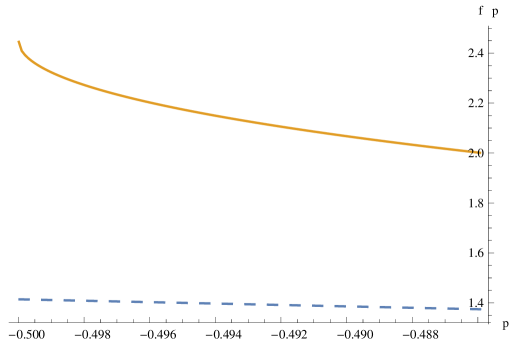
Figure 2: The MVCI of $\varrho_{2}$ (dashed line) v.s. the MVCI after Local filtering (solid line). $f(p)$ stands for the MVCI. Note that the classical bound of the CHSH inequality is $2$.

Remark: In [17] Horodeckis have presented the connection between the maximal violation of the CHSH inequality and the optimal quantum teleportation fidelity:

$$\mathcal{F}_{max}\geq\frac{1}{2}(1+\frac{1}{12}\max_{\mathcal{B_{CHSH}}}|\langle{\mathcal{B_{CHSH}}}\rangle_{\rho}|)$$ (25)

which means that any two-qubit quantum state violating the CHSH inequality is useful for teleportation and vice versa. Ac$\acute{i}$n et al. have derived the relation between the maximal violation of the CHSH inequality and the Holevo quantity between Eve and Bob in device-independent Quantum key distribution(QKD)[18]:

$$\chi(B_{1}:E)\leq h(\frac{1+\sqrt{(\max_{\mathcal{B_{CHSH}}}|\langle{\mathcal{B_{CHSH}}}\rangle_{\rho}|/2)^{2}-1}}{2}),$$ (26)

where $h$ is the binary entropy. From our theorem, $\max_{\mathcal{B_{CHSH}}}|\langle{\mathcal{B_{CHSH}}}\rangle_{\rho}|$ can be enhanced by implementing a proper local filtering operation from smaller to larger than $2$, which makes a teleportation possible from impossible, or can be improved to obtain a better teleportation fidelity. The proper(optimal) local filtering operation can be selected by the optimizing process in (9) together with the double cover relationship between the $SU(2)$ and $SO(3)$. For application in the QKD, Eve can enhance the upper bound of Holevo quantity by local filtering operations which makes a chance for attacking the protocol.

Discussions

It is a fundamental problem in quantum theory to recognize and explore the non-locality of a quantum system. The Bell inequalities and their maximal violations supply powerful ability to detect and qualify the non-locality. Furthermore, the constructing and the computation of the maximal violation of a Bell inequality is in close relationship with quantum games, minimal Hilbert space dimension and dimension witnesses, as well as quantum communications such as communication complexity, quantum cryptography, device-independent quantum key distribution etc. [6]. A proper local filtering operation can generate and enhance the non-locality. We have investigated the behavior of the maximal violations of the CHSH inequality and the V$\acute{e}$rtesi’s inequality under local filtering. We have presented an analytical method for any two-qubit system to compute the maximal violation of the CHSH inequality and the lower bound of the maximal violation of V$\acute{e}$rtesi’s inequality under local filtering. We have shown by examples that there exist quantum states whose nonlocality can be revealed by local filtering operations in terms of the V$\acute{e}$rtesi’s inequality instead of the CHSH inequality.

Methods

Proof of Theorem 1 and Theorem 2

The normalization factor $N$ has the following form,

$$N = tr[U\Sigma_{A}^{2}U^{{\dagger}}\otimes V\Sigma_{B}^{2}V^{{\dagger}}\rho]=tr[\Sigma_{A}^{2}\otimes\Sigma_{B}^{2}U^{{\dagger}}\otimes V^{{\dagger}}\rho U\otimes V]$$ (27)

$$= tr[\Sigma_{A}^{2}\otimes\Sigma_{B}^{2}\varrho],$$

where $\varrho=U^{{\dagger}}\otimes V^{{\dagger}}\rho U\otimes V$. Since $\rho$ and $\varrho$ are local unitary equivalent, they must have the same value of the maximal violation for CHSH inequality.

We have that

$$t^{\prime}_{ij} = tr[\rho^{\prime}\sigma_{i}\otimes\sigma_{j}]=\frac{1}{N}tr[(F_{A}\otimes F_{B})\rho(F_{A}^{{\dagger}}\otimes F_{B})^{{\dagger}}\sigma_{i}\otimes\sigma_{j}]$$ (28)

$$= \frac{1}{N}tr[\rho U\Sigma_{A}U^{{\dagger}}\sigma_{i}U\Sigma_{A}U^{{\dagger}}\otimes V\Sigma_{B}V^{{\dagger}}\sigma_{j}V\Sigma_{B}V^{{\dagger}}]$$

$$= \frac{1}{N}\sum_{kl}tr[U^{{\dagger}}\otimes V^{{\dagger}}\rho U\otimes V\Sigma_{A}O^{A}_{ik}\sigma_{k}\Sigma_{A}\otimes\Sigma_{B}O^{B}_{jl}\sigma_{l}\Sigma_{B}]$$

$$= \frac{1}{N}\sum_{kl}O^{A}_{ik}O^{B}_{jl}tr[\varrho\Sigma_{A}\sigma_{k}\Sigma_{A}\otimes\Sigma_{B}\sigma_{l}\Sigma_{B}]$$

$$= \frac{1}{N}\sum_{kl}O^{A}_{ik}O^{B}_{jl}tr[\varrho\delta_{k}\otimes\eta_{l}]$$

$$= \frac{1}{N}\sum_{kl}O^{A}_{ik}x_{kl}O^{B}_{jl}=\frac{1}{N}(O_{A}XO_{B}^{T})_{ij}.$$

In deriving the fourth equality in (28) we have used the double cover relation between the special unitary group $SU(2)$ and the special orthogonal group $SO(3)$: for any given unitary operator $U$, $U\sigma_{i}U^{{\dagger}}=\sum\limits_{j=1}^{3}O_{ij}\sigma_{j}$, where the matrix $O$ with entries $O_{ij}$ belongs to $SO(3)$ [25, 26].

Finally, one has that

$$T^{\prime}=\frac{1}{N}O_{A}XO_{B}^{{\dagger}},$$ (29)

and

$$(T^{\prime})^{{\dagger}}T^{\prime}=\frac{1}{N^{2}}O_{B}X^{{\dagger}}O_{A}^{{\dagger}}O_{A}XO_{B}^{{\dagger}}=\frac{1}{N^{2}}O_{B}X^{{\dagger}}XO_{B}^{{\dagger}}.$$ (30)

By noticing the orthogonality of the operator $O_{B}$ we have that the eigenvalues of $(T^{\prime})^{{\dagger}}T^{\prime}$ and $X^{{\dagger}}X/N^{2}$ must be the same, which proves theorem 1.

We can further obtain theorem 2 by substituting (29) into (5).  

Acknowledgements

This work is finished in the Beijing Computational Science Research Center and is supported by the NSFC Grants No. 11275131 and No. 11675113; the Shandong Provincial Natural Science Foundation No.ZR2016AQ06; the Fundamental Research Funds for the Central Universities Grants No. 15CX08011A and No. 16CX02049A; Qingdao applied basic research program No. 15-9-1-103-jch, and a project sponsored by SRF for ROCS, SEM.

Author contributions

M. Li and H.H. Qin wrote the main manuscript text. All authors reviewed the manuscript.

Additional Information

Competing Financial Interests: The authors declare no competing financial interests.

References

[1]Bell J.S. On the Einstein Podolsky Rosen Paradox. Physics1, 195-200 (1964).
[2] Brukner Č., Żukowski M. & Zeilinger A. Quantum Communication Complexity Protocol with Two Entangled Qutrits. Phys. Rev. Lett.89, 197901 (2002).
[3] Buhrman H., Cleve R., Massar S., & de Wolf R. Nonlocality and communication complexity. Rev.
Mod. Phys.82, 665 (2010).
[4] Scarani V., & Gisin N. Quantum Communication between N Partners and Bell’s Inequalities. Phys. Rev. Lett.87, 117901 (2001).
[5] Ekert A.K. Phys. Rev. Lett. Quantum cryptography based on Bell s theorem. 67, 661(1991); Barrett J.,Hardy L.
& Kent A. Phys. Rev. Lett. No Signaling and Quantum Key Distribution. 95, 010503 (2005).
[6] Brunner N., Cavalcanti D., Pironio S., Scarani V., & Wehner S. Bell nonlocality. Rev. Mod. Phys.86, 419 (2014).
[7] Clauser J.F., Horne M.A., Shimony A., & Holt R.A. Proposed Experiment to Test Local Hidden-Variable Theories. Phys. Rev. Lett.23, 880 (1969).
[8] Gisin N.
Bell’s inequality holds for all non-product states. Phys. Lett. A154, 201-202 (1991).
[9] Gisin N. & Peres A. Maximal violation of Bell’s inequality for arbitrarily large spin. Phys. Lett. A162, 15-17 (1992).
[10] Popescu S. & Rohrlich D. Generic quantum nonlocality. Phys. Lett. A166, 293-297 (1992).
[11]Chen J.L., Wu C.F., Kwek L.C., & Oh C.H. Gisin’s Theorem for Three Qubits. Phys.
Rev. Lett.93, 140407 (2004).
[12]Li M. & Fei S.M. Gisin s Theorem for Arbitrary Dimensional Multipartite States. Phys. Rev. Lett.104, 240502 (2010).
[13]Yu S.X., Chen Q., Zhang C.J., Lai C.H. & Oh C.H. All entangled pure states violate a single Bell’s
inequality. Phys. Rev. Lett.109, 120402 (2012).
[14] Horodecki R., Horodecki P. & Horodecki M. Violating Bell inequality by mixed spin-12 states: necessary and sufficient condition. Phys. Lett.
A200, 340 (1995).
[15]Vértesi T. More efficient Bell inequalities for Werner states. Phys. Rev. A 78, 032112 (2008).
[16] Degorre J., Laplante S., & Roland J. Simulating quantum correlations as a distributed sampling problem.
Phys. Rev. A72, 062314 (2005).
[17] Horodecki R., Horodecki M., & Horodecki P. Teleportation, Bell’s inequalities and inseparability. Phys. Lett. A222, 21 (1996).
[18] Acín A., Brunner N., Gisin N., Massar S., Pironio S., & Scarani V. Phys. Rev. Lett. Device-Independent Security of Quantum Cryptography against Collective Attacks. 98, 230501 (2007).
[19] Verstraete F., Dehaene J.,
& De Moor B. Normal forms and entanglement measures for multipartite quantum states. Phys. Rev. A68, 012103 (2003).
[20] Li M., Zhang T.G., Hua B., Fei S.M., & Li-Jost X.Q. Quantum Nonlocality of Arbitrary Dimensional Bipartite States. Scientific Reports5 13358 (2015).
[21] Verstraete F. & Wolf M.M. Entanglement versus Bell Violations and Their Behavior under Local Filtering Operations. Phys. Rev. Lett.89, 170401 (2002).
[23] Gisin N., Hidden quantum nonlocality revealed by local filters. Phys. Lett. A210, 151(1996).
[24] Peres A. Separability Criterion for Density Matrices. Phys. Rev. Lett.77, 1413 (1996).
[25] Schlienz J. & Mahler G. Description of entanglement. Phys. Rev. A52, 4396 (1995).
[26] Li M., Zhang T.G., Fei S.M., Li-Jost X.Q. & Jing N.H. Local Unitary Equivalence of Multi-qubit Mixed quantum States. Phys. Rev. A89, 062325 (2014).
[27]Werner R. F. Quantum states with Einstein-Podolsky-Rosen correlations admitting a hidden-variable
model. Phys. Rev. A40, 4277 (1989).